Probing gravity with a joint analysis of galaxy and CMB lensing and SDSS spectroscopy

Abstract

We present measurements of $E_{G}$, a probe of gravity from large-scale structure, using BOSS LOWZ and CMASS spectroscopic samples, with lensing measurements from SDSS (galaxy lensing) and Planck (CMB lensing). Using SDSS lensing and the BOSS LOWZ sample, we measure $\left\langle E_{G}\right\rangle=0.40^{+0.05}_{-0.04}$ (stat), consistent with the predicted value from the Planck $\Lambda\text{CDM}$ model, $E_{G}=0.46$. Using CMB lensing, we measure $\left\langle E_{G}\right\rangle=0.46^{+0.08}_{-0.09}$ (stat) for LOWZ (statistically consistent with galaxy lensing and Planck predictions) and $\left\langle E_{G}\right\rangle=0.39^{+0.05}_{-0.05}$ (stat) for the CMASS sample, consistent with the Planck prediction of $E_{G}=0.40$ given the higher redshift of the sample. We also study the redshift evolution of $E_{G}$ by splitting the LOWZ sample into two samples based on redshift, with results being consistent with model predictions. We estimate systematic uncertainties on the above $\left\langle E_{G}\right\rangle$ numbers to be $\sim 6$% (when using galaxy-galaxy lensing) or $\sim 3$% (when using CMB lensing), subdominant to the quoted statistical errors. These systematic error budgets are dominated by observational systematics in galaxy-galaxy lensing and by theoretical modeling uncertainties, respectively. We do not estimate observational systematics in galaxy-CMB lensing cross correlations.

1 Introduction

The standard $\Lambda$CDM model of cosmology has been successful in explaining a wide array of cosmological measurements (see Weinberg et al., 2013, for a review), from the early Universe (e.g., Steigman, 2010; Komatsu et al., 2011; Planck Collaboration et al., 2015a) down to $z\lesssim 1$ (e.g., Riess et al., 1998; Perlmutter et al., 1999; Kilbinger et al., 2013; Mandelbaum et al., 2013; Betoule et al., 2014; Alam et al., 2016a), though there are some mild tensions between different probes (see for example Planck Collaboration et al., 2015a; Riess et al., 2016). General relativity (GR) lies at the core of this model but it requires additional matter and energy components (dark matter and dark energy) to explain structure formation and cosmic acceleration. The nature of these components, especially dark energy, is not very well understood and this leaves open the possibility that the laws of gravity may require modifications as well (e.g., Jain & Khoury, 2010).

The theory of general relativity has been remarkably successful in explaining results over a wide range of scales (see Will, 2014, for a review of experimental tests of GR). On cosmological scales, it is possible to test the nature of gravity through several observables since gravity determines the dynamics and the growth of structure.

One important probe is the large scale velocity field, particularly the redshift space distortions (see Hamilton, 1997, for a review). Observationally, local motions (or peculiar velocities) of galaxies introduce errors in the distances inferred using the cosmological redshift-distance relation. Due to the coherent nature of the velocities, these errors then lead to detectable distortions in the otherwise isotropic correlation function (or power spectrum in Fourier space) of galaxies. These distortions in the redshift-space correlation function depend on the strength of gravitational attraction and are parameterized through the redshift- (or time-) dependent growth rate factor, $f(z)$. Several surveys have detected RSD and constrained $f(z)$ at different redshifts (e.g., Beutler et al., 2012; de la Torre et al., 2013; Alam et al., 2015b; Alam et al., 2016a) and used it to constrain gravity (Jennings et al., 2011; Alam et al., 2016b).

Gravitational lensing is another probe of the large scale structure. Gravitational lensing results from deflections in the path of photons by the gravitational potential of intervening matter, as they travel from the source to the observer (Bartelmann & Schneider, 2001; Kilbinger, 2015). In the weak regime, lensing introduces small but coherent distortions in the shapes of galaxies. Correlations between the shapes of background galaxies can thus be used to study the gravitational potential of foreground matter. Similarly, in the case of the CMB, lensing remaps the background anisotropies, leading to cross-correlations between different modes that can be exploited to recover the matter potential (Zaldarriaga & Seljak, 1999; Hu & White, 2001; Lewis & Challinor, 2006). Cross-correlations between galaxies and the lensing maps from CMB (galaxy-CMB lensing) or background galaxies (galaxy-galaxy lensing) can be used to study the galaxy-matter cross-correlations as well as the evolution of the structure over cosmic time scales (e.g., Massey et al., 2007; Hirata et al., 2008; Mandelbaum et al., 2013; Kilbinger et al., 2013; Heymans et al., 2013; Planck Collaboration et al., 2015b; Giannantonio et al., 2016). These measurements can then also be used to test the laws of gravity as well, since growth of structure and the lensing effect itself depends on the nature of gravity (e.g., Simpson et al., 2013).

Zhang et al. (2007) suggested the probe, $E_{G}$, as a consistency check on the theory of gravity by combining RSD measurements with the galaxy-lensing cross correlations (see also Leonard et al., 2015). $E_{G}$ is sensitive to the “gravitational slip” or the ratio of Newtonian potential and curvature potential, which are equal within GR in the absence of any anisotropic stress. $E_{G}$ has been measured by Reyes et al. (2010), Blake et al. (2016), de la Torre et al. (2016), Alam et al. (2017a) and Amon et al. (2018) using galaxy-galaxy lensing and by Pullen et al. (2016) using galaxy-CMB lensing. These measurements are largely consistent with the $\Lambda\text{CDM}$ predictions, though Pullen et al. (2016) measured $E_{G}$ to be $\sim 2.6\sigma$ lower than the predictions, with most of the discrepancy coming from the low CMB lensing amplitude at large scales.

In this work, we measure $E_{G}$ using the BOSS galaxy samples and SDSS galaxy lensing as well as Planck CMB lensing maps. In the case of galaxy lensing, due to limitations of the SDSS sample we only use the BOSS low redshift sample (LOWZ) while for CMB lensing we use both LOWZ and CMASS samples.

Throughout, we use the Planck 2015 cosmology (Planck Collaboration et al., 2015a), with $\Omega_{m}=0.309$, $n_{s}=0.967$, $A_{s}=2.142\times 10^{-9}$, $\sigma_{8}=0.82$. To get predictions for the matter correlation function, we use the linear power spectrum with halofit (Smith et al., 2003; Takahashi et al., 2012), generated using the CAMB software (Lewis & Bridle, 2002b).

2 Formalism and Estimators

In this section we provide a brief review of the theoretical formalism and the estimators used in this work.

2.1 Weak Lensing

As photons travel from their sources to observers, their paths are deflected by the structure in the intervening matter distribution (see Bartelmann & Schneider, 2001; Kilbinger, 2015; Mandelbaum, 2017, for reviews). The lensing potential of a given lensing mass depends on the lens potential and the geometric factors involving distances between the lens, source and observer, and is given by

$$\Phi_{L}=\int\mathrm{d}\chi_{l}\frac{f_{k}(\chi_{s}-\chi_{l})}{f_{k}(\chi_{s})f_{k}(\chi_{l})}\Psi(f_{k}(\chi_{l})\mathbf{\theta},\chi_{l})$$ (1)

$\chi_{l}$ and $\chi_{s}$ are line-of-sight distances to lens and source respectively ($\chi_{s}>\chi_{l}$), $\mathbf{\theta}$ is the angular separation between the lens and source on the sky and $f_{k}(\chi)$ is the transverse comoving distance ($f_{k}(\chi)=\chi$ in a flat universe). The Weyl potential $\Psi$ is given by

$$\Psi=\psi+\phi$$ (2)

$\psi$ and $\phi$ are the Newtonian and curvature potentials. Within $\Lambda\text{CDM}$, $\psi=\phi$ in the absence of any anisotropic stress. The main focus of this paper is to test this equality of the two potentials through the measurement of the $E_{G}$ parameter as defined in Section 2.5.

In the case where the angular extent of source is much smaller than angular scales over which lens potential varies, the distortion matrix relating the source and observer planes is given by

$$A=\begin{bmatrix}1-\kappa-\gamma_{1}&-\gamma_{2}\\ -\gamma_{2}&1-\kappa+\gamma_{1}\end{bmatrix}.$$

where $\gamma=\gamma_{1}+i\gamma_{2}=|\gamma|e^{i2\phi}$ is the shear in the observer frame and can be rotated to the lens-source frame to give $\gamma=\gamma_{t}+i\gamma_{\times}$. For a circularly symmetric lens, the convergence $\kappa$ and the tangential shear $\gamma_{t}$ are given by

$$\kappa(r_{p})=\frac{\Sigma(r_{p})}{\Sigma_{c}}$$ (3)

$$\gamma_{t}(r_{p})=\frac{\Delta\Sigma}{\Sigma_{\text{crit}}}=\frac{\overline{\Sigma}(<r_{p})-\Sigma(r_{p})}{\Sigma_{c}}$$ (4)

while $\gamma_{\times}=0$ due to symmetry. $\Sigma$ is the projected surface mass density and $\overline{\Sigma}(<r_{p})$ is the mean $\Sigma$ within radius $r_{p}$ from lens center. For non-circularly symmetric lens distributions, the equation is true when averaging within annuli at fixed $r_{p}$. The geometric factor $\Sigma_{\text{crit}}$ is given by

$$\Sigma_{\text{crit}}=\frac{c^{2}}{4\pi G}\frac{f_{k}(\chi_{s})}{(1+z_{l})f_{k}(\chi_{l})f_{k}(\chi_{s}-\chi_{l})}.$$ (5)

$1+z_{l}$ converts the $c^{2}/G$ factor to comoving space. The projected surface mass density can be written in terms of the 2-point galaxy-matter cross correlation function (lensing is sensitive to density fluctuations, not the mean density)

$$\Sigma(r_{p})=\bar{\rho}_{m}\int\mathrm{d}\Pi\,\xi_{gm}(r_{p},\Pi)=\bar{\rho}_{m}w_{gm}(r_{p}),$$ (6)

$\bar{\rho}_{m}$ is the mean matter density in comoving coordinates. Under the assumption of large projection length $\Pi$, the projected galaxy-matter cross correlation function $w_{gm}$ can be derived from the matter power spectrum as

$$w_{gm}(r_{p})=b_{g}A_{l}r_{\text{cc}}\int\mathrm{d}z\,W(z)\int\frac{\mathrm{d}^{2}k}{(2\pi)^{2}} P_{\delta\delta}(\mathbf{k},z)e^{i(\mathbf{r}_{p}\cdot\mathbf{k})}$$ (7)

$W(z)$ is the lens weight function, that we compute using the weights defined in Sections 2.1.1 and 2.1.2. $b_{g}$ is the galaxy bias, $r_{cc}$ is the galaxy-matter cross correlation coefficient and $A_{l}$ is the scale independent lensing amplitude. Details of modeling the lensing measurements will be presented in a separate work (Singh et. al in prep). In this work we will derive the correction in $E_{G}$ for the effects of $r_{\text{cc}}$ and non-linear galaxy bias from mocks as detailed in section 2.6 and section 4.2.

2.1.1 Estimator: Galaxy-galaxy lensing

We measure the $\Delta\Sigma$ using tangential shear as

$$\widehat{\Delta\Sigma}(r_{p})=B_{L}(1+m_{\gamma})\frac{\sum_{ls}w_{ls}e_{t}^{(ls)}\Sigma_{\text{crit}}^{(ls)}}{2\mathcal{R}\sum_{rs}w_{rs}}-\frac{\sum_{rs}w_{rs}e_{t}^{(rs)}\Sigma_{\text{crit}}^{(rs)}}{2\mathcal{R}\sum_{rs}w_{rs}}$$ (8)

where the summations are over all the lens-source (ls) or random lens-source (rs) pairs, where random lenses are unclustered random points with the same sky coverage and redshift distribution as the real lens galaxies. The signal measured around random lenses is subtracted to remove the spurious signal from additive systematics (Mandelbaum et al., 2005). As demonstrated in Singh et al. (2016a), subtraction of the signal around random points also leads to a more optimal estimator with better covariance properties. Note that the normalization factor uses weights computed using randoms. This is to account for the source galaxies that are associated with the lens and are not lensed, but enter the estimator due to the scatter in photometric redshifts. The lens-source pair weights are given by

$$w_{ls}=w_{l}\frac{\Sigma_{\text{crit}}^{-2}}{\sigma_{\gamma}^{2}+\sigma_{SN}^{2}}.$$ (9)

$\Sigma_{\text{crit}}^{-2}$ enters because we have defined $\widehat{\Delta\Sigma}$ as the maximum likelihood estimator (Sheldon et al., 2004); $\sigma_{SN}$ is the shape noise and $\sigma_{\gamma}$ is the measurement noise. $w_{l}$ is the weight for lens galaxies, defined in section 3.3.

As described in section 3.2, we also multiply the ellipticity with shear responsivity $\mathcal{R}$ to get ensemble shear estimates and measured signal with the correction factors for photometric redshifts ($B_{L}\sim$1.1) and for the shear biases ($1+m_{\gamma}\sim$1.04).

2.1.2 Estimator: Galaxy-CMB lensing

Using CMB lensing, we measure the projected surface mass density as (Singh et al., 2016b)

$$\widehat{\Sigma}(r_{p})=\frac{\sum_{lp}w_{lp}\kappa_{p}\Sigma_{c,{*}}}{\sum_{lp}w_{lp}}-\frac{\sum_{Rp}w_{Rp}\kappa_{p}\Sigma_{c,{*}}}{\sum_{Rp}w_{Rp}}$$ (10)

where the summation is over all the lens-pixel (pixels of CMB convergence map) pairs at separations $r_{p}\in[r_{p,min},r_{p,max}]$ at the lens redshift and the signal around randoms is subtracted to remove the effects of the correlated convergence, in the measurement (Singh et al., 2016b).

The weight for each lens-pixel pair is given by

$$w_{lp}=w_{l}\Sigma_{c,*}^{-2}.$$ (11)

We have defined $\widehat{\Sigma}$ as the maximum likelihood estimator, similar to galaxy-galaxy lensing, and $\Sigma_{c,*}$ is $\Sigma_{\text{crit}}$ with CMB as the source.

2.2 Projected galaxy clustering

The two-point galaxy correlation function in redshift space can be written as

$$\xi_{gg}(r_{p},\Pi,z)= b_{g}^{2}\int\frac{\mathrm{d}^{2}k_{\perp}\mathrm{d}k_{z}}{(2\pi)^{3}}P_{\delta\delta}(\mathbf{k},z)\left(1+\beta\mu^{2}\right)^{2}e^{i(\mathbf{k}_{\perp}\cdot\mathbf{r}_{p}+k_{z}\Pi)}$$ (12)

where $P_{\delta\delta}$ is the matter power spectrum; $r_{p},k_{\perp}$ are the separation and Fourier vector in the plane of the sky while $\Pi,k_{z}$ are the separation and Fourier vector along the line-of-sight. $b_{g}$ is the linear galaxy bias and the $(1+\beta\mu^{2})$ factor accounts for the linear redshift space distortions (Kaiser, 1987, see also Section 2.3), where $\beta=f(z)/b_{g}$ and $f(z)\approx\Omega_{m}(z)^{0.55}$ is the linear growth rate (effects of non-linear RSD on projected correlation functions are negligible and hence we ignore them). The projected correlation function is then

$$w_{gg}(r_{p})= \int\mathrm{d}z\,W(z)\int_{-\Pi_{\text{max}}}^{\Pi_{\text{max}}}\mathrm{d}\Pi\,\xi_{gg}(r_{p},\Pi,z)$$ (13)

$\Pi_{\text{max}}$ is the maximum line-of-sight separation for which the correlation function is computed. The weight function accounts for the differential contribution from different redshifts to the correlation function. It depends on total volume as well as redshift distribution of the galaxies, $p(z)$, and is given by (Mandelbaum et al., 2011)

$$W(z)=\frac{p(z)^{2}}{\chi^{2}(z)\mathrm{d}\chi/\mathrm{d}z}\left[\int\frac{p(z)^{2}}{\chi^{2}(z)\mathrm{d}\chi/\mathrm{d}z}\mathrm{d}z\right]^{-1}$$ (14)

Note that $W(z)$ can also be written in terms of comoving number density of galaxies, $n(z)$, as $W(z)\propto n(z)^{2}dV$. Finally the projected correlation function can be written as

$$w_{gg}(r_{p})=\frac{b^{2}}{\pi^{2}}\int\mathrm{d}zW(z)\int_{0}^{\infty}\mathrm{d}k_{z}\int_{0}^{\infty}\mathrm{d}k_{\perp}\frac{k_{\perp}}{k_{z}}P_{\delta\delta}(\mathbf{k},z)$$

$$\sin(k_{z}\Pi_{\text{max}})J_{0}(k_{\perp}r_{p})\left(1+\beta\mu^{2}\right)^{2}$$ (15)

where $J_{0}$ is the zeroth order Bessel function.

2.2.1 Estimator

To measure the galaxy clustering, we use the generalized Landy-Szalay estimator (Landy & Szalay, 1993)

$$\xi_{gg}=\frac{(D-R)(D-R)}{RR}=\frac{DD-2DR+RR}{RR},$$ (16)

where $D$ is the weighted galaxy sample, with weights defined in section 3.3 and $R$ is for the random sample (corresponding to the weighted galaxy catalog).

The projected correlation function can then be obtained by integrating the correlation function along the line-of-sight

$$w_{gg}=\int^{\Pi_{\text{max}}}_{-\Pi_{\text{max}}}\xi_{gg}(r_{p},\Pi)\,\mathrm{d}\Pi.$$ (17)

$\Pi_{\text{max}}$ denotes the size of top hat window function along the line-of-sight. It is desirable to use a larger $\Pi_{\text{max}}$ to mitigate the effects of redshift space distortions in the projected correlation function, though very large line-of-sight ($\Pi$) values add little signal and mostly contribute noise (for a survey of finite window size in redshift). We use $\Pi_{\text{max}}=100h^{-1}\text{Mpc}$, though we also test our results using $\Pi_{\text{max}}=50h^{-1}\text{Mpc}$ and $\Pi_{\text{max}}=200h^{-1}\text{Mpc}$, finding consistent results.

2.3 Redshift space distortions

The measured redshift ($z$) of the galaxy is a combination of Hubble recession and the peculiar velocity. The peculiar velocity component of the redshift affects the line-of-sight distance to a galaxy determined using the cosmological distance-redshift relation, introducing an anisotropy in the two-point correlation function. Within linear theory, the real space power spectra can be converted to redshift space power spectra as (Kaiser, 1987)

$$P_{gg}^{s}(\mathbf{k})=P_{gg}^{r}(\mathbf{k})(1+\mu_{k}^{2}\beta)^{2}.$$ (18)

where $P_{gg}^{r}$ is the real space galaxy power spectrum, $P_{gg}^{s}$ is the redshift space galaxy power spectrum, $\mu$ is the cosine of the angle made by the wave-vector $\mathbf{k}$ from the line-of-sight and $\beta$ is the RSD parameter. Hamilton (1992) extended this approach to the two-point correlation function and showed that the linear theory two-point correlation function in redshift space is given by

$$\xi_{gg}(\mathbf{s})=\left[1+f(\partial/\partial z)^{2}(\nabla^{2})^{-1}\right]^{2}\xi_{gg}(\mathbf{r})$$ (19)

where $\xi_{gg}(\mathbf{r})$ and $\xi_{gg}(\mathbf{s})$ are the galaxy correlation function in real and redshift space. The development of perturbation theories has produced better models of redshift space correlation that work even in the quasi-linear scales (Bernardeau et al., 2002; Crocce & Scoccimarro, 2006; Chan et al., 2012; Crocce et al., 2012). They enable interpretation of RSD measurements to smaller separations, and hence result in more precise measurements of RSD (Samushia et al., 2014). There are also efforts to model non-linear scales using HOD Reid et al. (2014a), by combining N-body simulations with Eulerian perturbation theory Hand et al. (2017) and using higher order LPT calibrated with N-body simulations Song et al. (2018). We use Convolution Lagrangian Perturbation Theory (CLPT) to predict the real space correlation function and velocity moments, which are then combined with the Gaussian Streaming Model (GSM) to predict the redshift-space correlation function (Carlson et al., 2013; Wang et al., 2014). We use tools developed in Alam et al. (2015b) which have been tested on several mocks and N-body simulations including the completed cosmological analysis of DR12 from BOSS (Satpathy et al., 2016; Alam et al., 2016a). Our formalism ignores the impact of gravitational lensing and generalized Sachs-Wolfe effects on the two point clustering which are shown to be negligible at the level of current precision (Yoo, 2009).

2.3.1 Measuring the growth rate

We estimate $\beta$ using the monopole and quadruple moments of the galaxy auto-correlation function, obtained by projecting the redshift space correlation function onto the Legendre basis.

$$\xi_{gg,l}(s)=\int_{-1}^{1}\mathrm{d}\mu\,\mathcal{P}_{l}(\mu)\xi_{gg}(s,\mu)$$ (20)

where $s$ is the distance in redshift space, $\mu$ is the angle between $\mathbf{s}$ and the plane of the sky and $\mathcal{P}_{l}$ is the Legendre polynomial of order $l$ ($l=0$ for monopole and $l=2$ for quadrupole).

We use COSMOMC (Lewis & Bridle, 2002a) to run a Markov Chain Monte Carlo (MCMC) fit for the multipole moments of the correlation function. The correlation function is fit for 3 parameters ($f,\sigma_{FOG},\nu$), where $f$ is the growth rate, $\sigma_{FOG}$ is an additional velocity dispersion to model the Finger of God effect (Reid et al., 2012; Alam et al., 2015b) and $\nu$ is the over-density which determines the first and second order bias through the peak-background split (White, 2014):

$$F^{\prime} =\frac{1}{\delta_{c}}\left[a\nu^{2}-1+\frac{2p}{1+(a\nu^{2})^{p}}\right]$$ (21)

$$F^{\prime\prime} =\frac{1}{\delta_{c}^{2}}\left[a^{2}\nu^{4}-3a\nu^{2}+\frac{2p(2a\nu^{2}+2p-1)}{1+(a\nu^{2})^{p}}\right]$$ (22)

where a = 0.707, p = 0.3 gives the Sheth-Tormen mass function (Sheth & Tormen, 1999), and $\delta_{c}=1.686$ is the critical density for collapse. $F^{\prime}$ and $F^{\prime\prime}$ are the first and second order Lagrangian bias. The linear galaxy bias is given by $b_{g}=1+F^{\prime}$. The RSD fits use scales from 35 to 70 $h^{-1}$Mpc. The minimum scale is chosen to only use the scales where the model is shown to be consistent with survey mocks and N-body simulations (Alam et al., 2015b), whereas the maximum scale is determined by the size of the jackknife regions that we use to estimate the covariance (see section 2.7).

2.4 $\Upsilon$ Estimator

In galaxy-galaxy lensing, we measure $\Delta\Sigma=\overline{\Sigma}(<r_{p})-\Sigma(r_{p})$. $\overline{\Sigma}(<r_{p})$ and hence $\Delta\Sigma$ is affected by all scales $<r_{p}$. This induces considerable theoretical uncertainty in modeling the $\Delta\Sigma$ observable due to the lack of a good model for the small scales, for example, non-linear clustering and galaxy-dark matter cross-correlations (usually quantified through the $r_{\text{cc}}$ parameter) at scales comparable to or within the virial radii of dark matter halos. To mitigate the impact of small-scale theoretical uncertainty on large-scale structure measurements, Baldauf et al. (2010) suggested a new estimator

$$\Upsilon_{gm}(r_{p},r_{0})=\Delta\Sigma_{gm}(r_{p})-\frac{r_{0}^{2}}{r_{p}^{2}}\Delta\Sigma(r_{0})$$ (23)

Expanding $\Delta\Sigma$ in terms of the correlation function, it can be shown that $\Upsilon$ is independent of information from small scales, $r<r_{0}$:

$$\Upsilon_{gm}(r_{p},r_{0})=\bar{\rho}_{M}\left[\frac{2}{r_{p}^{2}}\int_{r_{0}}^{r_{p}}\mathrm{d}r^{\prime}\,w_{gm}(r^{\prime})-\right.\\ \left.w_{gm}(r_{p})+\frac{r_{0}^{2}}{r_{p}^{2}}w_{gm}(r_{0})\right].$$ (24)

Analogous to this lensing observable, we can define $\Upsilon_{gg}$, starting by defining

$$\Sigma_{gg}(r_{p})={\rho}_{\text{crit}}\int\mathrm{d}\Pi\,\xi_{gg}(r_{p},\Pi),$$ (25)

where we have ignored the effects of the mean density and $\rho_{\text{crit}}$ is used to get $\Sigma_{gg}$ in units of density. The choice of $\rho_{\text{crit}}$ is also useful for the definition of the $E_{G}$ parameter in Section 2.5. The definition of $\Upsilon_{gg}$ follows from the definition of $\Delta\Sigma$ and Eq. (23).

2.5 $E_{G}$ Statistic

The perturbed metric in the conformal Newtonian gauge is written as

$$ds^{2}=a(\tau)^{2}\{-(1+2\psi)d\tau^{2}+(1-2\phi)(dr^{2}+r^{2}d\Omega^{2})\}$$ (26)

As stated in section 2.1, $\psi=\phi$ in $\Lambda\text{CDM}$, in the absence of anisotropic stresses. However, several modified gravity theories lead to modifications in either or both the potentials and in general violate the equality of two potentials (Jain & Khoury, 2010).

Zhang et al. (2007) proposed an estimator, $E_{G}$, to test the equality of two metric potentials

$$E_{G}(k,z)=\frac{P_{g\kappa}(k,z)}{P_{g\theta}(k,z)}$$ (27)

The projected real-space analog of $E_{G}$ was defined by Reyes et al. (2010) (see also Leonard et al. 2015) as

$$E_{G}(r_{p})=\frac{\Upsilon_{gm}(r_{p})}{\beta\Upsilon_{gg}(r_{p})}$$ (28)

Equivalently, we can define $E_{G}$ in terms of projected surface mass density

$$E_{G}(r_{p})=\frac{\Sigma_{gm}(r_{p})}{\beta\Sigma_{gg}(r_{p})}$$ (29)

In the case of galaxy-galaxy lensing, we will measure $E_{G}$ using $\Upsilon$ estimators, while for CMB lensing we will present results using both $\Upsilon$ and $\Sigma$. $\Sigma$ provides a more accurate and precise measurement at small scales as there is no mixing of scales or removal of information as in $\Delta\Sigma$ or $\Upsilon$. However, $\Sigma$ has lower signal to noise ($S/N$) at large scales due to the low amplitude and higher contribution from cosmic variance, which introduces a noise bias in $E_{G}$ (because we take the ratio of quantities with low $S/N$), in addition to the measurement being noisy. $\Upsilon$ on the other hand has lower $S/N$ at small scales but is better at large scales due to higher $S/N$.

$E_{G}$ is sensitive to the difference between $\psi,\phi$ as $P_{g\kappa}$ or $\Upsilon_{gm}$, measured from lensing, are sensitive to the Weyl potential ($\Psi=\psi+\phi$), while the linear growth rate of matter perturbations depends on the Newtonian potential $\psi$. In $\Lambda$CDM, with $\psi=\phi$

$$E_{G}(r_{p},z)=\frac{\Omega_{m}(z=0)}{f(z)}$$ (30)

In this paper we focus on measurements of $E_{G}$ and their implications for the $\Lambda\text{CDM}$ model. We do not test for any specific models of modified gravity, and refer the reader to Pullen et al. (2015) for $E_{G}$ predictions in some alternate theories of gravity.

2.6 $E_{G}$ corrections

Theoretically, in the linear regime, $E_{G}$ is a clean null test for the equality of the two metric potentials and hence a test of GR. However, it can be subject to some of the systematics that we discuss here.

Non-linear clustering at small scales can lead to significant deviations from the expected value of $E_{G}$, especially since it affects lensing and clustering measurements differently. The clustering ($\Upsilon_{gg}$) amplitude goes as $b_{g}^{2}$, which includes difficult-to-model non-linear galaxy bias. Lensing ($\Upsilon_{gm}$) is sensitive to $b_{g}r_{cc}$, where $b_{g}$ includes non-linear bias while $r_{\text{cc}}$ is the galaxy-matter cross correlation coefficient. $r_{\text{cc}}\sim 1$ at large scales but deviates strongly at small scales and depends on details of how galaxies populate halos (see e.g. Baldauf et al., 2010, for more detailed discussion on $r_{cc}$). As discussed in Baldauf et al. (2010), use of $\Upsilon$ rather than $\Delta\Sigma$ partially mitigates the effects of non-linear clustering by removing small-scale information, though the efficiency of this small-scale removal depends on the choice of $r_{0}$. The choice of $r_{0}$ depends on the balance between theoretical uncertainties, which are large at small scales, and statistical errors, which increase with $r_{0}$ as more signal is removed. For our main analysis, we choose $r_{0}=2h^{-1}\text{Mpc}>2r_{\text{vir}}$, as suggested by Baldauf et al. (2010). This still leaves some residual effects from non-linear scales and we attempt to mitigate these effects by estimating them using simulations. For this we compute the correction factor $C_{nl}$, in real space, to correct for the effects of scale-dependent bias and $r_{cc}$.

$$C_{nl}(r_{p})=\frac{\Upsilon_{gg}^{\text{sim}}(r_{p})}{b_{\text{linear}}\Upsilon_{gm}^{\text{sim}}(r_{p})}$$ (31)

$b_{\text{linear}}$ is the linear galaxy bias.

The finite size of the top-hat window function in the clustering measurement leaves some residual effects of linear redshift space distortions in the projected correlation function (see also Section 2.2.1) and hence in the $E_{G}$ measurement. The lensing measurement is not affected by RSD to first order and also the implicit line-of-sight integration in lensing is much longer ($\Pi_{\text{max}}^{\text{lens}}\gg 100h^{-1}\text{Mpc}$). We mitigate the effect of the limited window in projected clustering using the corrections computed with the linear theory and Kaiser formula (Kaiser, 1987).

$$C_{\text{rsd+win}}(r_{p})=\frac{w_{gg}(r_{p}|\Pi_{\text{max}}=100h^{-1}\text{Mpc})}{w_{gg}(r_{p}|\Pi_{\text{max}}=\infty)}$$ (32)

where $w_{gg}$ is defined in Eq. (15).

In addition to the above, the window function for lensing (depends on the broad lensing kernel and systematics weights) also varies, due to which effective weights to different $\Pi$ bins are different for lensing and clustering. We correct for this effect using simulations by computing $\Upsilon_{gm}$ separately with top hat weights and lensing weights which also includes the lens-source pair weights defined in Section 2.1.

$$C_{\text{lens win}}(r_{p})=\frac{\int d\Pi\,\xi_{gm}(r_{p},\Pi)}{\int d\Pi\,\mathcal{W}_{gm}(\Pi)\,\xi_{gm}(r_{p},\Pi)}$$ (33)

Here $\mathcal{W}_{gm}$ is the lensing window function derived in Appendix A.

Due to different redshift weights for lensing and clustering, the two measurements are also at different effective redshifts. Since the lensing amplitude scales as $b_{g}D(z)^{2}$ ($D(z)$ is the linear growth function) and clustering amplitude scales as $b_{g}^{2}D(z)^{2}$, we correct for the different effective redshifts as

$$C_{z}(r_{p})=\frac{D(z=z_{\text{eff}}^{gg})}{D(z=z_{\text{eff}}^{gm})}\sqrt{\frac{\int dz\mathcal{W}_{gg}(z)w_{gg}(r_{p},z)}{\int dz\mathcal{W}_{gm}(z)w_{gg}(r_{p},z)}}$$ (34)

The ratio is directly computed from the data by measuring clustering with lensing weights ($\mathcal{W}_{gm}$) assigned to the galaxies and is in general scale-dependent as different scales grow differently with redshift under the effects of non-linear physics. The ratio of growth function is computed from the theoretical model at fiducial cosmology. Within linear theory, this correction leads to cancellation the redshift dependent factors from projected clustering and lensing and the final measurement is at the effective redshift of measured growth rate $f$, which has the effective redshift of clustering.

There are also additional number density fluctuations due to the lensing effects of the intervening large scale structure between the observer and galaxies (Moradinezhad Dizgah & Durrer, 2016). We estimate the impact of these effects in appendix B and apply a correction $C_{\text{lens}}$.

We estimate and show these corrections in section 4.2. The final correction applied to the measured $E_{G}$ signal is the product of all corrections defined above.

$$C_{\text{tot}}(r_{p})=C_{\text{lens win}}(r_{p})\times C_{nl}(r_{p})\times C_{\text{rsd+win}}(r_{p})\times C_{z}(r_{p})\times C_{\text{lens}}$$ (35)

2.7 Covariance

To compute the covariance matrix for both clustering and lensing measurements, we split the sample into 100 jackknife regions with approximately equal area on the sky. Singh et al. (2016a) showed that the jackknife errors are consistent with theoretical expectations when using mean zero quantities, i.e., galaxy field with mean subtracted using randoms, as for the lensing and clustering estimators in this work. Throughout, the quoted errors and uncertainties will be jackknife errors. Whenever fitting models or computing derived quantities such as $E_{G}$ (or a mean), we do so for each jackknife region separately using the diagonal entries of the jackknife covariance and then quote the jackknife mean and errors of model parameters. Lensing measurements are dominated by shape noise on the scales that contribute the most information, so using diagonal covariance for lensing and $E_{G}$ is justified (covariance of $E_{G}$ is dominated by lensing). However, the use of a diagonal covariance matrix can lead to biased parameter and error estimation when the bins are strongly correlated due to incorrect weighting applied to the bins. Similar biases can also arise when inverting noisy covariance matrices, which are accounted for (but not corrected for) by Hartlap factor (Hartlap et al., 2007; Taylor et al., 2013) by increasing the size of errors. In our work this issue is most relevant for the measurement of the RSD parameters from the clustering measurement, where the differences in the mean value from using the full versus diagonal jackknife covariance can be $\sim 0.5\sigma$ and the errors when using the diagonal covariance are also overestimated by $\sim 10\%$. Thus for RSD, we fit each jackknife region separately, but using the full covariance matrix estimated using all regions. Also, for the errors quoted on the parameters, we do not apply the Hartlap factor, which is close to 0.84 for our analysis and will increase the quoted errors by $\sim 8\%$. Since for deriving $\left\langle E_{G}\right\rangle$ we use only the diagonal covariance with the average over the jackknife, it is not clear whether Hartlap factor is the right correction to use and hence we do not apply it to our results. If we make a simplifying assumption that the uncertainty in each bin is estimated independently of the other bins, then the Hartlap factor in each bin is the same as that for the case with one data point; this correction factor is $\sim 1.5\%$ for 100 jackknife regions.

3 Data

We use the same datasets as used in Singh et al. (2016b). In this section, we briefly describe these datasets for completeness.

3.1 SDSS

We use imaging and spectroscopic datasets from the SDSS-I,II and III surveys (Gunn et al., 1998; York et al., 2000; Eisenstein et al., 2001; Richards et al., 2002; Strauss et al., 2002; Gunn et al., 2006). The SDSS-I/II survey was completed in the seventh data release (Abazajian et al., 2009) though the data reduction pipeline was improved by (Padmanabhan et al., 2008) in the eighth data release (Aihara et al., 2011), which is used to derive our imaging catalogs as described in the next section.

3.2 Galaxy lensing: Shape sample

The catalogue of galaxies with measured shapes used in this paper (described in Reyes et al. 2012 and further characterized in Mandelbaum et al. 2013) was generated using the re-Gaussianization method (Hirata & Seljak, 2003) of correcting for the effects of the point-spread function (PSF) on the observed galaxy shapes. The catalogue production procedure was described in detail in previous work, so we describe it only briefly here. Galaxies were selected in a 9243 deg² region, with an average number density of $1.2$ arcmin^-2 based on requiring shape measurements in both $r$ and $i$ bands. The selection was based on cuts on the imaging quality, data reduction quality, galactic extinction $A_{r}<0.2$ defined using the dust maps from Schlegel et al. (1998) and the extinction-to-reddening ratios from Stoughton et al. (2002), apparent magnitude (extinction-corrected $r<21.8$ using model magnitudes), and galaxy size compared to the PSF. For comparing the galaxy size to that of the PSF, we use the resolution factor $R_{2}$ which is defined using the trace of the moment matrix of the PSF $T_{\mathrm{P}}$ and of the observed (PSF-convolved) galaxy image $T_{\mathrm{I}}$ as

$$R_{2}=1-\frac{T_{\mathrm{P}}}{T_{\mathrm{I}}}.$$ (36)

We require $R_{2}>1/3$ in both $r$ and $i$ bands.

The basic principle of shear measurement using these images is to fit a Gaussian profile with elliptical isophotes to the image, and define the components of the ellipticity

$$(e_{+},e_{\times})=\frac{1-(b/a)^{2}}{1+(b/a)^{2}}(\cos 2\phi,\sin 2\phi),$$ (37)

where $b/a$ is the axis ratio and $\phi$ is the position angle of the major axis. The ensemble average ellipticity is then an estimator for the shear,

$$(\gamma_{+},\gamma_{\times})=\frac{1}{2\cal R}\langle(e_{+},e_{\times})\rangle,$$ (38)

where ${\cal R}\approx 0.87$ is called the ‘shear responsivity’ and represents the response of the distortion to a small shear (Kaiser et al., 1995; Bernstein & Jarvis, 2002); ${\cal R}\approx 1-e_{\mathrm{rms}}^{2}$.

For this work, we do not use the entire source catalogue, only the portion overlapping the LOWZ sample.

When computing the weak lensing signals around the LOWZ galaxies, we need estimates of the redshifts for the fainter source galaxies. For this purpose, we use the maximum-likelihood estimates of photometric redshifts (photo-$z$) based on the five-band photometry from the Zurich Extragalactic Bayesian Redshift Analyzer (ZEBRA, Feldmann et al., 2006), which were characterized by Nakajima et al. (2012) and Reyes et al. (2012). Following Nakajima et al. (2012), we use a representative calibration sample of source galaxies with spectroscopic redshifts to calculate biases in weak lensing signals due to bias and scatter in the photo-$z$, and applied corrections that were of order 10 per cent ($\pm 2$ per cent) to the weak lensing signals (we multiply the final lensing measurement with 1.1 and the 2 percent uncertainty is added to the systematics error budget). We further test the accuracy of these corrections using the clustering-redshift method (e.g., Ménard et al., 2013) in appendix D.

As discussed in Mandelbaum et al. (2017), new shear calibration simulations that include the impact of nearby neighbors on the shear estimates from re-Gaussianization identified a previously uncorrected effect due to those neighbors. Since the shear calibration simulations that were originally used to quantify shear systematic errors in the SDSS catalog used in this work (Mandelbaum et al., 2012) did not include nearby neighbors, we must include this newly-identified correction in our results in this work. Figure 18 in Mandelbaum et al. (2017) clearly illustrates that this correction is a function of the depth of the sample used for shear estimation. For SDSS-like depths, the correction is a factor of $1.04\pm 0.02$. We apply the 1.04 correction to our LOWZ lensing measurements, and fold the $\pm 0.02$ into our systematic error budget.

3.3 SDSS-III BOSS

The BOSS spectroscopic survey was performed using the BOSS spectrograph (Ahn et al., 2012; Smee et al., 2013) with targets selected from the SDSS photometric catalogs (Dawson et al., 2013) and data processed by automated pipelines (Blanton et al., 2003; Bolton et al., 2012). We use SDSS-III BOSS data release 12 (Alam et al., 2015a; Reid et al., 2016) and select LOWZ galaxies in the redshift range $0.16<z<0.36$ and CMASS galaxies in $0.45<z<0.7$.

The LOWZ sample consists of Luminous Red Galaxies (LRGs) at $z<0.4$ and is approximately volume-limited in the redshift range we use, $0.16<z<0.36$, with a number density of $\bar{n}\sim 3\times 10^{-4}~{}h^{3}\text{Mpc}^{-3}$ (Manera et al., 2015; Reid et al., 2016). To test for the redshift evolution of $E_{G}$, we also split the sample into two redshift bins, Z1: $0.16<z<0.26$ and Z2: $0.26<z<0.36$. Further, we also use a sample of field galaxies (Singh et al., 2016b) defined using the counts-in-cylinders (CiC) technique (Reid & Spergel, 2009). Field galaxies are mainly central galaxies and have somewhat lower bias and hence are relatively less affected by non-linear bias effects.

The BOSS CMASS sample consists of higher redshift galaxies ($0.45<z<0.7$) targeted using color and magnitude cuts intended to select a uniform sample of massive galaxies (Reid et al., 2016). The use of apparent color and magnitude to select targets may affect the selected galaxy sample due to relativistic effects. Alam et al. (2017c) showed that impact of such effects are negligible for the CMASS sample.

We also use the weights defined by the BOSS collaboration (Ross et al., 2012) for systematics ($w_{\text{sys}}$), redshift failures ($w_{\text{no-z}}$) and fiber collisions ($w_{\text{cp}}$). The effects of these weights for both clustering and lensing measurements were studied in detail in Singh et al. (2016b) (see also Ross et al., 2012; Anderson et al., 2014). The final weights are defined as

$$w=w_{\text{sys}}(w_{\text{no-z}}+w_{\text{cp}}-1)$$ (39)

3.4 Planck CMB lensing maps

For CMB lensing, we use the publicly available lensing maps from Planck collaboration (Planck Collaboration et al., 2015b). We convert the provided convergence values in Fourier space $\kappa_{\ell,m}$ into real space $\kappa_{\theta,\phi}$ using healpy (Górski et al., 2005) with $n_{\text{side}}=1024$. We use the full $\ell$ range ($8<\ell<2048$) when constructing the map. Planck Collaboration et al. (2015b) found some evidence of systematics in lensing maps and use $40<\ell<400$ for the main cosmological analysis. However, in Singh et al. (2016b) no evidence of systematics was found when cross-correlating the full convergence map with the BOSS galaxies and hence we will use the full $\ell$ range in this work as well, though we will quote the number using scales corresponding to $\ell<400$ cut. We refer the reader to Singh et al. (2016b) for more details about choice of pixel size in the maps and various systematic tests that were carried out.

3.5 Simulations

To test our $E_{G}$ pipeline and compute the corrections described in section 2.6, we use the ‘Med-Res’ simulations described in Reid et al. (2014b), with snapshots at $z=0.25$ and $z=0.40$ for the LOWZ sample and $z=0.60$ for the CMASS sample. The sample of galaxies is generated using the HOD model from Zheng et al. (2005) to fit the clustering of galaxies for full LOWZ or CMASS samples, assuming a fixed abundance of halos (see Reid et al., 2014b, for more details). We will use same simulation catalogs to compute corrections for the subsamples as well. To compute the galaxy-matter cross-correlations, we cross-correlate the galaxies with the randomly subsampled matter particles.

4 Results

In this section we presents the results, starting with growth rate measurements in the data, then $E_{G}$ measurements in simulations and tests for systematics and then the $E_{G}$ measurements in the data.

Sample	Lensing	$z_{\text{eff}}$	$f\frac{\sigma_{8}}{\sigma_{8,fid}}$	$E_{G}$
	map
Z1	SDSS	$0.21$	$0.75_{-0.088}^{+0.097}$ [$0.64$]	$0.38_{-0.061}^{+0.052}$ [$0.48$]
Z1	Planck	$0.21$	$0.75_{-0.088}^{+0.097}$ [$0.64$]	$0.6_{-0.113}^{+0.112}$ [$0.48$]
Lowz	SDSS	$0.27$	$0.62_{-0.056}^{+0.055}$ [$0.66$]	$0.4_{-0.038}^{+0.046}$ [$0.46$]
lowz-pl	Planck	$0.27$	$0.62_{-0.056}^{+0.055}$ [$0.66$]	$0.46_{-0.088}^{+0.082}$ [$0.46$]
Field	SDSS	$0.27$	$0.62_{-0.056}^{+0.055}$ [$0.66$]	$0.4_{-0.039}^{+0.042}$ [$0.46$]
Field	Planck	$0.27$	$0.62_{-0.056}^{+0.055}$ [$0.66$]	$0.47_{-0.079}^{+0.077}$ [$0.46$]
Z2	SDSS	$0.32$	$0.5_{-0.065}^{+0.063}$ [$0.69$]	$0.45_{-0.073}^{+0.08}$ [$0.45$]
Z2	Planck	$0.32$	$0.5_{-0.065}^{+0.063}$ [$0.69$]	$0.4_{-0.1}^{+0.115}$ [$0.45$]
CMASS	Planck	$0.57$	$0.69_{-0.07}^{+0.066}$ [$0.77$]	$0.4_{-0.051}^{+0.049}$ [$0.4$]
CMASS	Planck		$r_{p}\in[25,150]$	$0.38_{-0.064}^{+0.065}$ [$0.4$]

Table 1: Values of the growth function, $f$, and $E_{G}$ for different samples and using SDSS and Planck CMB lensing maps. The values in square brackets, $[]$, are the predicted values from the Planck $\Lambda\text{CDM}$ model. $z_{\text{eff}}$ is the effective redshift of galaxy clustering measurements (Galaxy-lensing cross correlations have different $z_{\text{eff}}$ for which we apply $C_{z}$ correction to $E_{G}$). The errorbars in this table are statistical only. There is additional systematic uncertainty of order $\sim 3\%$ in measurements using Planck CMB lensing maps and $\sim 6\%$ in measurements using SDSS galaxy lensing. The systematic uncertainties include contributions of order $2\%$ from the applied corrections and $\sim 2\%$ on RSD modeling (Alam et al., 2017a) (modeling uncertainties). In addition, measurements using SDSS galaxy lensing have a further $5-6\%$ systematic uncertainty from shear calibrations ($\sim 2\%$) and photometric redshifts ($\sim 5\%$). We do not estimate observational systematic uncertainties in CMB lensing maps. Note that for the field sample, we use $f$ measured from the full LOWZ sample. Due to the selection effects from CiC method, $f$ from the field sample is somewhat biased ($f=0.74\pm 0.05$). In the last row we have quoted the $E_{G}$ measurement using scales $25<r_{p}<150$$h^{-1}\text{Mpc}$, which corresponds approximately to the range of scales ($40<\ell<400$) used by Pullen et al. 2016 in their $E_{G}$ measurement.

4.1 Growth rate measurement

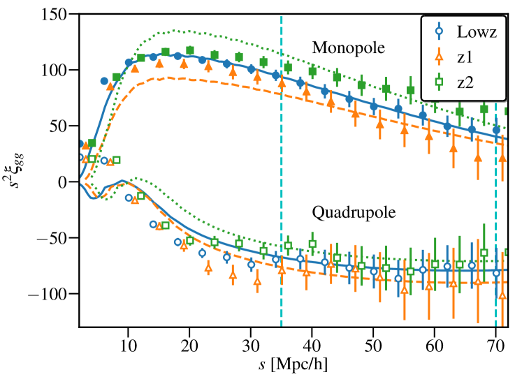
We performed the RSD analysis as described in Section 2.3. For every sample, monopole and quadruple moments in each jackknife region are fit independently using our perturbation theory model. The measurements and model fits are shown in figure 1 and the growth rate measurements are presented in table 1, with the results being consistent with $\Lambda$CDM predictions to within $\sim 1\sigma$.

Our RSD analysis is performed with a fixed cosmology because the constraints on cosmological parameters from Planck are tight enough that using Planck priors is nearly equivalent to fixing the cosmology. Our measurements of the growth rate are consistent with previous measurements using the SDSS sample (Alam et al., 2015b; Sánchez et al., 2014; Samushia et al., 2014; Satpathy et al., 2016; Beutler et al., 2016; Grieb et al., 2016; Sanchez et al., 2016; Alam et al., 2016a). We do not marginalize over the Alcock-Paczynski parameter and hence obtain smaller error than when doing the full shape RSD analysis (see for example Alam et al. 2015b). Sánchez et al. (2014) reported $f\sigma_{8}(z=0.32)=0.48\pm 0.10$ and $f\sigma_{8}(z=0.57)=0.42\pm 0.045$ using the SDSS DR11 sample, which is consistent with our LOWZ ($f\sigma_{8}(z=0.27)=0.44$) and CMASS ($f\sigma_{8}(z=0.57)=0.42$). A more detailed comparison of RSD modeling used in this paper with several other methods is shown in Alam et al. (2016a). Gil-Marín et al. (2016) presented one of the first RSD analysis which uses both power spectrum and bi-spectrum and their reported $f\sigma_{8}$ is consistent with ours for both LOWZ and CMASS sample. Our LOWZ measurement of $f\sigma_{8}$ is 0.5$\sigma$ lower than Gil-Marín et al. (2016) with fixed Alcock-Paczynski parameter but higher than what they measured after marginalizing over Alcock-Paczynski parameters. The lower $f\sigma_{8}$ after AP marginalization is dominated by the information in the position of the BAO peak. We do not use the BAO scale in our RSD analysis and hence do not allow extra freedom on top of the $\Lambda$CDM background when estimating $f\sigma_{8}$. We also note that in our model the growth rate ($f$) and additional velocity dispersion ($\sigma_{FOG}$) are uncorrelated with each other for small values of $\sigma_{FOG}$ but positively correlated for large values of $\sigma_{FOG}$. Therefore galaxy sample with stronger finger-of-god effect will show stronger effect on the growth rate constraint when marginalized over $\sigma_{FOG}$. We found that our $f\sigma_{8}$ constraint for LOWZ sample are not strongly affected by marginalizing over $\sigma_{FOG}$ but for the CMASS sample the error on growth rate increases by a factor of 2 when marginalizing over $\sigma_{FOG}$ compared to when it is fixed (the mean value of $f$ shifts by less than $0.2\sigma$). This can plausibly be explained by the fact that the volume occupied by CMASS sample is bigger and therefore gives a stronger constraint on $f\sigma_{8}$ which makes it easier to see the impact of marginalizing over $\sigma_{FOG}$.

The systematic uncertainty in our RSD model is estimated to be $\sim 2\%$ as reported in Alam et al. (2017a) while using scales above 25 $h^{-1}\text{Mpc}$. But, our sample extends to slightly lower redshift compared to previous analysis and hence we decided to use a slightly higher minimum scale in our RSD fits hoping to keep the systematic error at the same level. We used scales above 35 $h^{-1}\text{Mpc}$  in our measurement of $\beta$ whereas our final $E_{G}$ measurements extends to scales below 35 $h^{-1}\text{Mpc}$. Ideally one would want to perform measurement of $\beta$ using the same scales. Unfortunately the modeling technique used in the current measurement of $\beta$ is not accurate enough to extend it to smaller scales. The $\beta$ consists of two quantities growth rate and bias. We do account for the fact that bias will be scale dependent and different at smaller scales compared to the large scale measurement through a correction factor $C_{nl}$ (see Section 2.6 for details). But we have an inherent assumption that the growth rate measured using larger scales is constant and applicable for smaller scales. This makes the current measurements of $E_{G}$ slightly weaker than its full potential which should be improved upon in the future measurements with better RSD modeling to smaller scales.

Figure 1: For different subsamples of the LOWZ sample in the two panels, we show the multipole moments – the monopole ($l=0$) and quadrupole ($l=2$) of the galaxy correlation function, along with the best-fitting model (solid lines). The vertical dashed lines mark the range within which the model was fit, $35<r_{p}<70h^{-1}\text{Mpc}$

4.2 $E_{G}$ in simulations and corrections

In Fig. 2 we show the $E_{G}$ measurements in the simulation box with snapshots at $z=0.25$ and $z=0.4$, in both real space and redshift space. Without applying any corrections, $E_{G}$ is biased low with considerable scale dependence. The average $E_{G}$, $\left\langle E_{G}\right\rangle$, over all scales is low by $\sim 5\%$ compared to the $\Lambda\text{CDM}$ predictions both in real space and redshift space. RSD effects are important at large scales, but due to relatively lower $S/N$ these scales do not contribute much when computing the mean $E_{G}$. Still we do correct for these effects as described in Section 2.6. The biggest contribution to the bias in $E_{G}$ is from the combined effects of non-linear galaxy bias and the galaxy matter cross-correlation coefficient. We compute this bias, $C_{nl}$ directly from simulations and then correct for it.

Figure 2: $E_{G}$ measurements using simulations. Points with errorbars show the measurements, while dashed black lines show $\Lambda\text{CDM}$ predictions at two redshifts. Vertical cyan lines mark the scales $5<r_{p}<70h^{-1}\text{Mpc}$ within which we measure the $\left\langle E_{G}\right\rangle$ (not shown). Blue points show the measurements using real space positions for galaxies while orange points show measurements in redshift space. Open markers show measurements without any corrections applied while closed markers show results obtained after applying all corrections. We find that the most important correction is for the combined effects of non-linear bias and $r_{\text{cc}}$ (see eq. (31)). The corrections terms for the LOWZ sample are shown in Fig. 5.

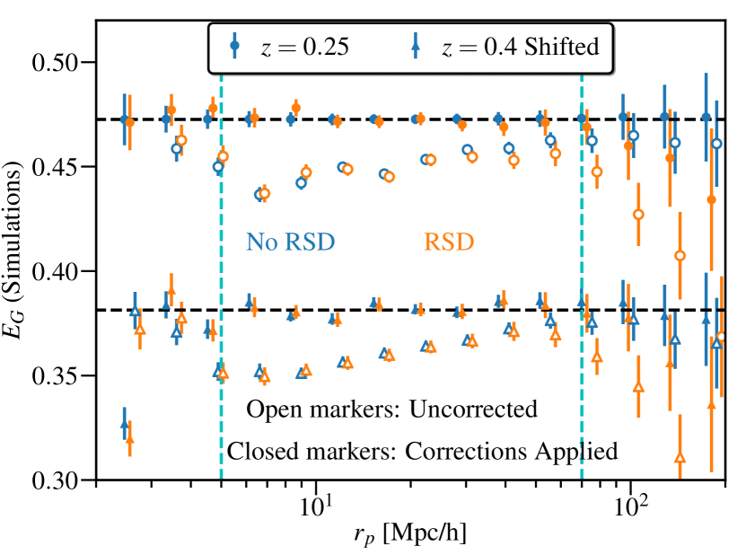
The $\left\langle E_{G}\right\rangle$ computed after applying the corrections, is within $\sim 1\%$ of the predicted value from the $\Lambda\text{CDM}$ model (compared to $5\%$ bias in the uncorrected $\left\langle E_{G}\right\rangle$). A primary concern about these corrections is that they may depend on the details of HOD modeling and hence may not be very accurate. In appendix C, we provide more tests using another set of mocks with varying HODs and show that the corrections used for our main results ($z=0.25$ snapshot) recover $\left\langle E_{G}\right\rangle$ to within $\lesssim 2\%$. Thus for our main results in the data, we will use the corrections from the $z=0.25$ snapshot for both the full LOWZ and LOWZ-Z1 samples, the $z=0.40$ snapshot for the LOWZ-Z2 sample and $z=0.6$ snapshot for the CMASS sample. To account for the variations in these corrections, we also add $2\%$ systematic uncertainty in our error budget.

4.3 $E_{G}$ measurement

Figure 3: $E_{G}$ as a function of scale for LOWZ galaxies. The dashed black line shows the Planck $\Lambda\text{CDM}$ prediction at $z=0.27$, while the solid lines show measured $\left\langle E_{G}\right\rangle$ over scales $5<r_{p}<70h^{-1}\text{Mpc}$. The bands show the $1\sigma$ errors on $\left\langle E_{G}\right\rangle$, averaged using the diagonal errors. Note that the galaxy lensing and CMB lensing are at different effective redshift due to lensing weights, with galaxy lensing cross correlations at $z_{\text{eff}}=0.24$ and CMB lensing cross correlations at $z_{\text{eff}}=0.3$. We apply correction $C_{z}$ to get final $E_{G}$ at effective redshift of clustering, $z=0.27$.

Figure 4: $E_{G}$ measurement for the CMASS sample with CMB lensing. We show the measurement using the $\Upsilon$ ($r_{0}=2h^{-1}\text{Mpc}$) estimator as well as using $\Sigma$, for both CMB lensing and clustering. $\Sigma$ provides a better $S/N$ at small scales, while $\Upsilon$ has better $S/N$ at large scales due to reduced cosmic variance (Baldauf et al., 2010). The green band shows the measurement of the mean $E_{G}$ from Pullen et al. 2016, using the same datasets but in Fourier space, over the effective scale range $25$–$150h^{-1}\text{Mpc}$. The dashed black line shows the Planck $\Lambda\text{CDM}$ prediction.

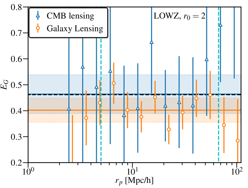
In Fig. 3, we show the $E_{G}$ measurement using the BOSS LOWZ sample along with both SDSS and CMB lensing maps. Using galaxy lensing, $\left\langle E_{G}\right\rangle$ is $\sim 1.5\sigma$ low compared to Planck $\Lambda\text{CDM}$ predictions, which is primarily driven by the low amplitude of lensing measurements (which gets compensated partially by low $f$). In the case of CMB lensing, $\left\langle E_{G}\right\rangle$ is consistent with Planck $\Lambda\text{CDM}$ predictions, though the measurement is noisier when compared to galaxy lensing. While the two measurements are statistically consistent, we note that galaxy-lensing ($z_{\text{eff}}=0.24$) and CMB-lensing $z_{\text{eff}}=0.3$ cross correlations are at different effective redshifts due to the impact of lensing weights and hence we apply different $C_{z}$ corrections to get them at effective redshift of clustering sample.

$E_{G}$ measured from the field sample is consistent with the results from the full LOWZ sample (using the same corrections for both). Since the field sample does not contain groups, the effects of non-linear bias and satellite contamination to the RSD measurement as well as to ratio of lensing and clustering (via its effects on $r_{\text{cc}}$) are expected to be smaller. However, with the CiC cylinder size of $r_{p}\lesssim 0.8h^{-1}\text{Mpc}$, we do not observe any significant effects of removing groups at scales $r_{p}>5h^{-1}\text{Mpc}$, other than a reduced effective bias of the sample. CiC selection effects still bias the RSD measurements and hence we do not use the $f=0.74\pm 0.05$ measured from the field sample.

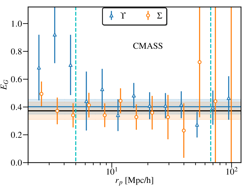
In Fig. 4, we show the $E_{G}$ measurement for the CMASS sample using the CMB lensing measurement with two estimators, $\Sigma$ and $\Upsilon$, for clustering and lensing measurements. Both measurements are consistent with Planck $\Lambda\text{CDM}$ predictions, though the mean $E_{G}$ measured from $\Sigma$ is noisier compared to $\Upsilon$ due to different signal to noise as a function of scale. At small scales, $\Sigma$ gives better signal-to-noise ratio ($S/N$) while at larger scales the $\Sigma$ measurement gets noisier. $\Upsilon$ on the other hand has lower $S/N$ at small scales since we are subtracting out some signal while at large scales it has better $S/N$ because of a reduced contribution from cosmic variance (see discussion in section 2.5). Note that corrections for CMASS sample are computed using the $z=0.6$ snapshot.

Figure 5: Various correction terms applied to the $E_{G}$ measurements in Fig. 3 (LOWZ sample). The black line also shows the relative uncertainty (rescaled by a factor of two) in $E_{G}$ as a function of scale. The per-bin uncertainty for galaxy lensing is of order 15–20% while for CMB lensing it is larger by a factor of 2 (30–40%)

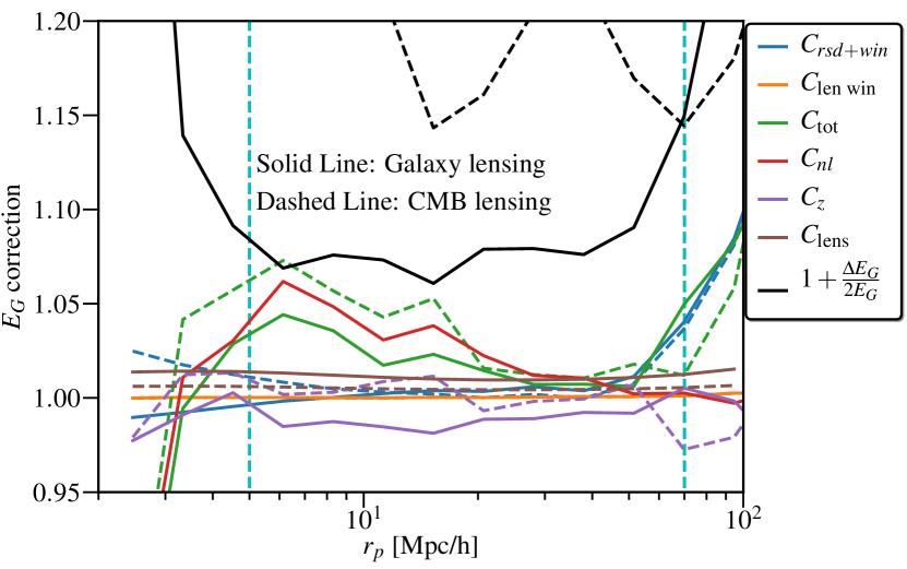
In Figure 5, we show the magnitude of several corrections applied to the LOWZ $E_{G}$ measurements along with the relative (statistical) errors in the $E_{G}$ measurement for comparison. The $C_{\text{rsd+win}}$ correction is computed from a theoretical model (linear theory$+$Kaiser correction). We also computed this correction using simulations (computing correlations with and without RSD) and find good agreement between theoretical estimates and simulations. Simulations are noisier, hence we use the theoretical estimates in the final results.

All the scale-dependent corrections we applied are subdominant when compared to the statistical uncertainties in the $E_{G}$ at that $r_{p}$, and the combined effect of corrections is to change $E_{G}$ by $\sim 1-2\%$ ($\lesssim 0.2\sigma$) for different samples. $C_{nl}$ is the largest net correction on $\left\langle E_{G}\right\rangle$ ($\sim 2-3\%$) as it affects small scales more with maximum values of order $5\%$, though it reduces rapidly as scale increases. $C_{rsd+win}$ has a small impact as it is close to one on small scales, though on larger scales (which are noisier and hence contribute less to $\left\langle E_{G}\right\rangle$) it can be of order $15\%$. $C_{rsd+win}$ is large on large scale because the correlation function has small values at large scales and RSD effects, which are primarily additive, can lead to large relative changes. The correction from the different effective $z$ of clustering and lensing, $C_{z}$, is of order $1-1.5\%$ on small scales and $\sim 0.1\%$ on the largest scales. The correction due to lensing magnification is $\sim 1-1.5\%$ and has only weak dependence with scale (see Figure 7) While these corrections do not lead to a significant change in our results, their magnitude suggests that future work with much higher $S/N$ measurements will have to model these corrections to higher precision.

Figure 6: $E_{G}$ measurement between scales $5<r_{p}<70$ $h^{-1}\text{Mpc}$ for different samples (this work), along with $\Lambda\text{CDM}$ predictions with different $\Omega_{m}$ values. Measurements in cyan are from other works, which may use a different range of scales. The measurements are consistent with the Planck $\Lambda\text{CDM}$ model ($\Omega_{m}=0.31$), though given the size of the statistical uncertainties, it is not possible to rule out other models. The blue band around the red points is drawn to indicate that the LOWZ measurement is correlated with the measurements from the Z1 and Z2 samples. Solid yellow points show the uncorrected value of $\left\langle E_{G}\right\rangle$ for the samples with measurements from this paper. Note that measurements from CMB and galaxy lensing are at different effective redshifts due to the impact of lensing weights and hence separate $C_{z}$ corrections are applied to $E_{G}$ using galaxy lensing and CMB lensing.

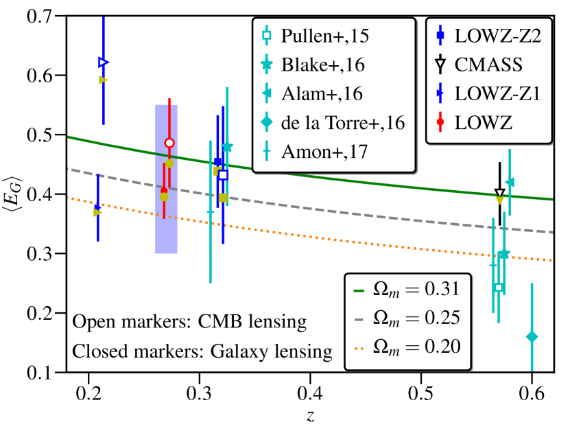
Finally, in Fig. 6, we show the redshift dependence of $\left\langle E_{G}\right\rangle$ along with $\Lambda\text{CDM}$ predictions using different values of $\Omega_{m}$. The values of $\left\langle E_{G}\right\rangle$ and $f$ are given in table 1. In general our measurements for various samples are consistent with the Planck $\Lambda\text{CDM}$ prediction at $2\sigma$ level or less. However the measurements are not sensitive enough to put meaningful constraints on modified gravity parameters or to even rule out lower values of $\Omega_{m}$, especially with galaxy-galaxy lensing measurements preferring somewhat lower values. For the full LOWZ and CMASS samples, our measurements are consistent with those of Blake et al. (2016) (using RCSlens and CFHTlens source galaxies), who measured $E_{G}=0.48\pm 0.10$ for LOWZ ($0.15<z<0.43$) and $E_{G}=0.30\pm 0.07$ for the CMASS sample, with the measurement of Alam et al. (2017a) (using CFHTlens source galaxies), $E_{G}=0.420\pm 0.056$, for CMASS sample and also with Amon et al. (2018) (using KiDS), $E_{G}=0.37\pm 0.12$ for LOWZ and $E_{G}=0.28\pm 0.08$ for CMASS sample.

The measured amplitude of $E_{G}$ is primarily affected by the (relative) lensing amplitude $A_{l}$ and the growth rate, $f$, measurement from RSD. In the case of galaxy-galaxy lensing, the lensing amplitude is lower than 1, which drives the measured $E_{G}$ to be lower than the $\Lambda\text{CDM}$  predictions. The lensing measurement from galaxies is susceptible to systematic uncertainties in shear estimation and photometric redshifts. As mentioned in Section 3.2, Reyes et al. (2012); Nakajima et al. (2012); Mandelbaum et al. (2013) did extensive testing of the shape sample for these systematics and we use the calibration factors derived for the shape sample derived in those papers, along with new corrections based on more recent simulations in HSC (Mandelbaum et al., 2017). We further test the accuracy of the calibration factors for photo-z in appendix D using a method with independent assumptions from the method used in Nakajima et al. (2012). There, the existence of a representative spectroscopic sample was assumed; here, we use the clustering redshift method, which assumes the existence of a non-representative spectroscopic sample that can be used to derive the ensemble redshift distribution by modeling the clustering signals. In appendix D we show that while the calibration factors from the clustering redshift method depend on the priors on the galaxy bias, they agree with the factors derived by Nakajima et al. (2012) to within $\sim 5\%$. Using physically-motivated priors on the galaxy bias further improves the agreement.

There is also a possibility of contamination from intrinsic alignments (IA) of source galaxies. Blazek et al. (2012) estimated the IA contamination in the source sample used in this work and found no evidence for contamination when measuring the shear signal around LRG lenses, with the conservative upper limit of the contamination being $5\%$. We thus ignore the possible contamination from IA in this work.

We also note that the (relative) lensing amplitude is degenerate with galaxy bias which is fixed from clustering, and lower apparent lensing amplitude does not necessarily mean systematics in lensing alone. Any systematics in the projected clustering, $w_{gg}$ , can also bias the $E_{G}$ estimation and can show up as low lensing amplitude if we are over estimating the clustering and hence the galaxy bias. Furthermore, systematics in clustering can also impact the measurements of growth rate which in turn impact the $E_{G}$. While we do not find very significant deviations in the growth rate measurements, there are order 10% variations in $f$ compared to the predictions from Planck $\Lambda\text{CDM}$ cosmology and they drive $E_{G}$ lower in case of $Z1$ sample and higher for $Z2$ and CMASS samples.

Another notable discrepancy is between our measurement for CMASS sample and that of Pullen et al. (2016). A significant part of the discrepancy in measurement of Pullen et al. (2016) (relative to Planck $\Lambda\text{CDM}$ prediction) is driven by large scales ($r_{p}\gtrsim 80h^{-1}\text{Mpc}$), where the galaxy-CMB lensing amplitude was observed to be lower than expected in their measurements. Our results, on the other hand, are dominated by the measurements at small scales, with larger scales being noisier and not contributing much to the mean $E_{G}$ measurement. Even when considering the full scale-dependent $E_{G}$ measurement, we do not observe any significant deviations at large scales, though the uncertainties in the measurement at those scales are rather large. Using the scales $25<r_{p}<150h^{-1}\text{Mpc}$, we measure $\left\langle E_{G}\right\rangle=0.33\pm 0.14$ using $\Sigma$ (statistically consistent with Pullen et al. (2016) measurement of $0.24\pm 0.06$ (stat) though errors are correlated between two studies) and $\left\langle E_{G}\right\rangle=0.38\pm 0.065$ using $\Upsilon$. We note we use slightly different redshift range $0.45<z<0.7$ compared to (Pullen et al., 2016) ($0.43<z<0.7$), but the volume in this range ($0.43<z<0.45$) is small, $<3\%$ of the sample, and is further down weighted due to rapidly decreasing number density of galaxies as well as the CMB lensing kernel and hence should not contribute significantly to the differences between the two studies. Also, since we use (optimal) $\Sigma_{\text{crit}}^{-2}$ weighting in the galaxy-lensing cross-correlations, the noise properties of the measurements in the two studies are somewhat different, though these differences should also be small. Another point to note is that Pullen et al. (2016) convert their scale-dependent measurement to a $\left\langle E_{G}\right\rangle$ using a maximum likelihood (MLE) method that requires inversion of a noisy covariance matrix. As a result the maximum likelihood point can be biased, which is accounted for by widening the likelihood using Hartlap factor and hence the uncertainty in $\left\langle E_{G}\right\rangle$. For our results, we measure the $\left\langle E_{G}\right\rangle$ in each jackknife region using only the diagonal covariance, which can also be suboptimal and introduce noise bias but we checked (by repeating the analysis with the full covariance) that it does not affect our results, as the off-diagonal elements of covariance matrix are expected to be subdominant. (This is because noise is dominated by CMB lensing reconstruction noise which acts as shot noise and hence the diagonal elements of covariance should be dominant in both configuration and Fourier space.) In essence, due to different treatment of noise in covariances, the results in the two studies may not be very correlated. Using the jackknife fitting with diagonal covariance on data from Pullen et al. (2016), we find $\left\langle E_{G}\right\rangle=0.29\pm 0.06$, which further rises higher to $\left\langle E_{G}\right\rangle=0.32\pm 0.06$ if we ignore the lowest $\ell$ bin ( $\ell\lesssim 70$) for which the errors are likely to be underestimated given the size of jackknife regions and also noise in error estimation (observed $S/N$ of this bin does not scale as the expected $\sqrt{(2\ell+1)\Delta\ell}$ scaling relative to neighboring bins). It is hard to further reconcile the measurements in the two works without doing additional tests that are outside the scope of this work.

5 Conclusions

We have presented the measurements of $E_{G}$ and its redshift dependence using BOSS galaxies and lensing measurements from SDSS galaxy lensing and Planck CMB lensing maps. Measurements from CMB lensing and galaxy lensing are consistent within the noise for the LOWZ lens sample. With the higher redshift CMASS sample, the $E_{G}$ measurement is of comparable significance to the galaxy lensing measurements for LOWZ sample. This highlights the potential of CMB lensing to provide complimentary observations and strong consistency checks when combined with the galaxy lensing measurements (see also Singh et al., 2016b; Schaan et al., 2016).

We also highlighted several theoretical uncertainties in computing $E_{G}$ on nonlinear scales, and computed corrections for them. Our results showed that after applying corrections in simulations we can recover $E_{G}$ to about $2\%$ accuracy. With $\gtrsim 10\%$ error in our measurement, these corrections are sufficient for this work. However, in the future, several surveys will be able to measure $E_{G}$ (or perform similar tests of GR) to sub-percent accuracy (Leonard et al., 2015; Pourtsidou, 2016). For these surveys, it will be important to compute the corrections for theoretical uncertainties to even higher accuracy, using better theoretical modeling with analytical models and/or simulations.

While our $E_{G}$ measurements are largely consistent with the predictions from Planck $\Lambda\text{CDM}$ predictions, there are some deviations at $\lesssim 2\sigma$ level, especially when using galaxy lensing measurements. Though statistically not very significant in $E_{G}$, these deviations are primarily driven by the low amplitude of lensing measurements, which can possibly be due to systematics in either clustering and/or lensing measurements, since clustering bias and lensing amplitude are degenerate. The lensing amplitude is also degenerate with the $\sim\sigma_{8}\Omega_{m}^{1/2}$ value, and low amplitude could also mean that data prefers lower $\Omega_{m}$ or $\sigma_{8}$ (or both) values compared to the Planck $\Lambda\text{CDM}$ model assumed. We also see similar redshift-dependent deviations in the growth rate measurements (and measurements with CMB lensing), though the uncertainties are too large to make a definitive statement. Since the growth rate is also degenerate with galaxy bias, this redshift-dependent deviation does suggest that it is possible that the problem (at least partly) is from the some residual sample selection effects which affect the galaxy clustering measurements.

Low amplitude lensing measurements (compared to predictions from Planck $\Lambda\text{CDM}$ model) have also been observed by other lensing studies (see for example Hildebrandt et al. (2016); Leauthaud et al. (2017); Joudaki et al. (2017); DES Collaboration et al. (2017) and for results consistent with Planck cosmology, van Uitert et al. 2017). Leauthaud et al. (2017) performed tests for effects of several systematics and the physics beyond $\Lambda\text{CDM}$ model in galaxy-galaxy lensing (eg. effects of baryonic physics, neutrinos, modified gravity, assembly bias, sample selection) and showed that such effects can be significant, especially with several systematics and physical effects being combined together. Joudaki et al. (2017) performed a similar analysis for cosmic shear measurements and also showed that marginalizing over some models for systematics can relieve some of the tensions between Planck $\Lambda\text{CDM}$ model and lensing measurements. These studies, along with our tests, suggest that more work is required to study and model the impact of systematics in both lensing and clustering measurements.

In the near future, data from the eBOSS, DES, KiDS and HSC surveys will help to extend the growth rate and $E_{G}$ measurements to higher redshifts with measurement uncertainties likely to be around $\lesssim 5\%$ level. With the advent of LSST, DESI, WFIRST, SKA and CMB Stage-IV surveys, the statistical uncertainties on $E_{G}$ will decrease considerably, providing percent level or better measurements. However, to make $E_{G}$ a strong test of gravity and $\Lambda\text{CDM}$ it is imperative to improve the modeling to mitigate observational systematics as well as theoretical uncertainties to much higher precision than was done in this work.

Appendix A Lensing window function

We define the window function as the weight assigned in the galaxy mass correlation function (Eq. (6)) at a given line-of-sight separation from lens galaxy. For a given lens-source pair, with a lens at $z_{l}$ and source at $z_{s}$ with photometric redshift $z_{p}$, the (unnormalized) window function is given by

$$w_{\text{win}}(\Pi|z_{l},z_{s},z_{p})=\Sigma_{\text{crit}}^{-2}(z_{l},z_{p})\int_{0}^{z_{s}}dz\,\Sigma_{\text{crit}}^{-1}(z,z_{s})\Sigma_{\text{crit}}(z_{l},z_{p})\delta_{D}\left(z-z_{l}-\frac{\Pi H(z_{l})}{c}\right)$$ (40)

where $\Pi$ is the line-of-sight separation from the lens. $\delta_{D}$ is the dirac delta function and enforces the correct relationship between $\Pi$ and $z$. $\Sigma_{\text{crit}}^{-2}(z_{l},z_{s})$ factor arises from the weights we used in $\Delta\Sigma$ estimator. $\Sigma_{\text{crit}}^{-1}(z,z_{s})$ is the true critical surface density at $z$ that weighs the contribution of matter fluctuation to shear, while $\Sigma_{\text{crit}}(z_{l},z_{p})$ is the critical surface density that we use to convert the shear back to matter density when measuring the signal. Since the two $\Sigma_{\text{crit}}$ factors are not the same, contributions from matter fluctuations at different redshifts are weighted differently in the correlation function leading to a non-trivial window function.

Integrating over the lens and source samples we get

$$w_{\text{win}}(\Pi)=\frac{1}{\mathcal{N}}\int dz_{l}P(z_{l})f_{k}(\chi_{l})^{-2}\int_{z_{l}}^{\infty}dz_{p}P(z_{p})\Sigma_{\text{crit}}^{-2}(z_{l},z_{p})\int_{0}^{2}dz_{s}P(z_{s}|z_{p})\int_{0}^{z_{s}}dz\Sigma_{\text{crit}}^{-1}(z,z_{s})\Sigma_{\text{crit}}(z_{l},z_{p})\delta_{D}\left(z-z_{l}-\frac{\Pi H(z_{l})}{c}\right)$$ (41)

where the normalization factor $\mathcal{N}$ is defined such that $w(\Pi=0)=1$. Also note that the effects of bias and scatter in photometric redshifts are included in the calibration biases derived in Nakajima et al. (2012) and hence we do not include them in our calculation. We set $P(z_{s}|z_{p})=\delta_{D}(z_{s}-z_{p})$ to get the final expression

$$w_{\text{win}}(\Pi)=\frac{1}{\mathcal{N}}\int dz_{l}P(z_{l})f_{k}(\chi_{l})^{-2}\int_{z_{l}}^{\infty}dz_{p}P(z_{p})\Sigma_{\text{crit}}^{-2}(z_{l},z_{p})\int_{0}^{z_{p}}dz\Sigma_{\text{crit}}^{-1}(z,z_{p})\Sigma_{\text{crit}}(z_{l},z_{p})\delta_{D}\left(z-z_{l}-\frac{\Pi H(z_{l})}{c}\right)$$ (42)

Appendix B Estimating lensing magnification bias to $E_{G}$

As shown by Moradinezhad Dizgah & Durrer (2016), the effects of lensing magnification modify the clustering and lensing observables and hence can bias the $E_{G}$ measurements. In this section we derive impact of our failure to model magnification bias on our real space clustering, lensing and $E_{G}$ observables.

B.1 Bias in Clustering

Due to the effect of lensing by the foreground structure, the apparent galaxy over-density is modified from the true over-density. This modification arises from two effects, the volume perturbations due to magnification, and the modification to the galaxy selection function (Yoo et al., 2009; Bernstein, 2009). Most previous studies have derived the magnification bias to clustering in Fourier space. In this section we derive the expression for magnification bias in projected clustering in real space with a limited line-of-sight window function.

Following the notation of Hildebrandt et al. (2009), to estimate the impact of lensing contamination on the galaxy clustering auto-correlation, we begin by assuming that the true number density of galaxies, $n_{0}$, for a given flux limit, $f$, follows a simple power-law relation

$$n_{0}(>f)=Af^{-\alpha},$$ (43)

where the slope $\alpha$ is measured as

$$\alpha=-\frac{d\log{(n_{0}(>f))}}{d\log{(f)}}=2.5\frac{d\log{(n_{0}(<m))}}{dm}.$$ (44)

where in the second equality we converted flux to the magnitude, $m$.

The magnification $\mu$ modifies the observed volume and the galaxy flux by $\frac{\widehat{V}}{V}=\frac{\widehat{f}_{g}}{f_{g}}\sim\mu$. Thus the observed number density of galaxies, $\widehat{n}$, changes due to the magnification $\mu$ as

$$\widehat{n}(>f)= \frac{V}{\widehat{V}}n_{0}(>\frac{f}{\mu})=\frac{1}{\mu}n_{0}(>\frac{f}{\mu})$$

$$= \frac{1}{\mu}\mu^{\alpha}n_{0}(>{f})$$

$$\widehat{n}(>f)\approx (1+2(\alpha-1)\kappa)n_{0}(>{f})$$ (45)

where we used the relation between magnification and convergence, $\kappa$, $\mu\approx 1/(1-\kappa)^{2}$.

The observed galaxy over-density, $\widehat{\delta}_{g}$, is then related to the true over-density, $\delta_{g}$, to first order as

$$\widehat{\delta}_{g}\approx\frac{(1+\kappa^{\prime})n_{g}}{\overline{n}_{g}}-1\approx\delta_{g}+\kappa^{\prime},$$ (46)

where $\kappa^{\prime}=2(\alpha-1)\kappa$.

The measured correlation function is then

$$\widehat{\xi}_{gg}(r_{p},\Pi) =\xi_{gg}(r_{p},\Pi)+\int dz\,W(z)\left\langle\kappa^{\prime}(z)\kappa^{\prime}{(z+\Delta z_{\Pi})}\right\rangle\left(\frac{r_{p}}{f_{k}(\chi_{z})}\right)$$

$$+\int dz\,W(z)\left\langle\delta_{g}(z)\kappa^{\prime}(z+\Delta z_{\Pi})\right\rangle(r_{p})+\int dz\,W(z)\left\langle\delta_{g}(z-\Delta z_{\Pi})\kappa^{\prime}(z)\right\rangle(r_{p})$$ (47)

where the integrals are over the redshift range of the galaxy sample. $\kappa^{\prime}(z)$ refers to the (magnification) convergence for a source at $z$, $\kappa^{\prime}(z)\kappa^{\prime}{(z+\Delta z_{\Pi})}(\frac{r_{p}}{f_{k}(\chi_{z})})$ is the convergence correlation function at angular separation $\theta=r_{p}/f_{k}(\chi_{z})$ for sources at $z$ and $z+\Delta z_{\Pi}$ and $\delta_{g}\kappa^{\prime}$ is the cross correlation between the galaxy over-density field and convergence. The projected correlation function is then

$$\widehat{w}_{gg}(r_{p}) =w_{gg}(r_{p})+\int_{-\Pi_{\text{max}}}^{\Pi_{\text{max}}}d\Pi\int dz\,W(z)\left\langle\kappa^{\prime}(z)\kappa^{\prime}{(z+\Delta z_{\Pi})}\right\rangle\left(\frac{r_{p}}{f_{k}(\chi_{z})}\right)$$

$$+\int_{-\Pi_{\text{max}}}^{\Pi_{\text{max}}}d\Pi\int dz\,W(z)\left\langle\delta_{g}(z)\kappa^{\prime}(z+\Delta z_{\Pi})\right\rangle(r_{p})$$ (48)

$$=w_{gg}(r_{p})+[2(\alpha-1)]^{2}\int_{-\Pi_{\text{max}}}^{\Pi_{\text{max}}}d\Pi\int dz\,W(z)\int_{0}^{z+\Delta z}d\chi_{m}\frac{\overline{\rho}_{m}^{2}w_{mm}\left(r_{p}\frac{f_{k}(\chi_{z_{m}})}{f_{k}(\chi_{z})},z_{m}\right)}{\Sigma_{\text{crit}}(z_{m},z)\Sigma_{\text{crit}}(z_{m},z+\Delta z)}$$

$$+2(\alpha-1)\int_{-\Pi_{\text{max}}}^{\Pi_{\text{max}}}d\Pi\int dz\,W(z){\overline{\rho}_{m}w_{gm}(r_{p},z)}\left(\frac{1}{\Sigma_{\text{crit}}(z,z+\Delta z)}+\frac{1}{\Sigma_{\text{crit}}(z-\Delta z,z)}\right)$$ (49)

where $\Delta z_{\Pi}=\frac{\Pi H(z)}{c}$ and $p_{g}(z)$ is the galaxy redshift distribution function. Under the assumption that $f(\chi_{z})\gg\Pi_{max}$, the last term can be approximated as

$$\int_{-\Pi_{\text{max}}}^{\Pi_{\text{max}}}d\Pi\int dz\,W(z){\overline{\rho}_{m}w_{gm}(r_{p},z)} \left(\frac{1}{\Sigma_{\text{crit}}(z,z+\Delta z)}+\frac{1}{\Sigma_{\text{crit}}(z-\Delta z,z)}\right)$$

$$\approx 2\int dz\,W(z)\overline{\rho}_{m}w_{gm}(r_{p},z)\frac{4\pi G(1+z)}{c^{2}}\int_{0}^{\Pi_{\text{max}}}d\Pi\frac{f_{k}(\chi_{z})\Pi}{f_{k}(\chi_{z})+\Pi}$$ (50)

$$=2\int dz\,W(z)\overline{\rho}_{m}w_{gm}(r_{p},z)\frac{4\pi G(1+z)}{c^{2}}\left[f_{k}(\chi_{z})\Pi_{\text{max}}-f_{k}(\chi_{z})^{2}\ln\left(\frac{f_{k}(\chi_{z})+\Pi_{\text{max}}}{f_{k}(\chi_{z})}\right)\right]$$

$$\approx 2\frac{3H_{0}^{2}\Omega_{m}}{2c^{2}}\frac{\Pi_{max}^{2}}{2}\int dz\,W(z)(1+z)w_{gm}(r_{p},z)$$ (51)

$$\approx 5\times 10^{-4}\int dz\,W(z)(1+z)w_{gm}(r_{p},z)$$

$$\approx 5\times 10^{-4}(1+\overline{z})w_{gm}(r_{p})$$ (52)

Note that our estimation of this term is $\sim 2$ orders of magnitude lower than the estimation by Moradinezhad Dizgah & Durrer (2016). This is likely driven by the different choice of $\Pi_{\text{max}}$, as Moradinezhad Dizgah & Durrer (2016) use $C_{\ell}$ where large effective line-of-sight integration length can give $\sim 2$ orders of magnitude difference in the contamination due to unmodeled magnification effects.

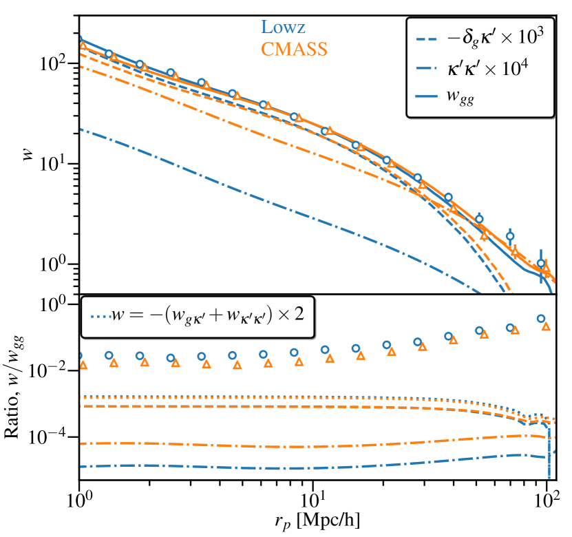
In Fig. 7(a) we show the estimated contamination from lensing to the clustering measurement for the case of both LOWZ and CMASS samples. We estimated $\alpha=0.4$ for LOWZ and $\alpha=0.5$ for CMASS using the slope of luminosity function on the fainter end. The dominant contribution is from ${\delta_{g}\kappa^{\prime}}$, which biases the clustering low by a factor of $\sim 10^{-3}$, much less than the statistical errors.

(a) Clustering

(b) Lensing

Figure 7: a) Lensing contamination to the clustering measurements. The upper panel shows the correlation function, $w_{gg}$, and the correlations due to lensing ${g\kappa^{\prime}}$ and ${\kappa^{\prime}\kappa^{\prime}}$. The lower panel shows the ratio of predicted contamination with the best fit model. The dotted lines in the lower panel are the total contamination from two terms, rescaled by a factor of two for clarity. Also, the open markers show the noise-to-signal ratio in the measurements. Note that in the upper panel (but not in lower panel, unless stated in lower panel legend), we multiplied lensing predictions with a constant factor to make them same order of magnitude as the clustering signal. b) Same as a), but showing the lensing contamination to $\Sigma$ and $\Delta\Sigma$ measurements.

B.1.1 Bias in redshift-space multipoles

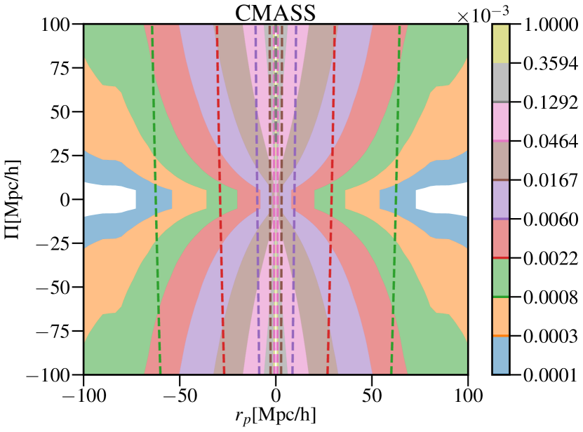
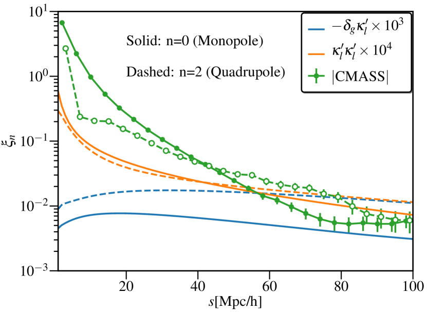
In Fig. 8(a) we show the magnification terms from Eq. (47) as a function of projected and line-of-sight separations. Due to the dependence of the lensing kernel on distances, these terms show anisotropic structure. The galaxy-magnification cross correlation increases at a given projected scale as the line-of-sight separation increases because the lensing kernel becomes more sensitive to the galaxies (i.e. the lensing kernel increases at the position of galaxies). The magnification auto-correlation increases with the mean redshift of the pair of galaxies, which increases with $\Pi$. As a result both of these terms also contribute to the multipoles of the correlation function, though as discussed in the previous section, these contributions are order $0.1\%$ or smaller when compared to the clustering signals. The monopole and quadrupole terms are shown in Fig. 8(b). In addition, these terms also have dipole contributions with the magnification autocorrelation being larger though it is smaller than the monopole by an order of magnitude.

(a)

(b)

Figure 8: a) Contamination from magnification to clustering as a function of projected and line-of-sight separations. Solid contours are the $\delta_{g}\kappa^{\prime}$ term with a negative sign and dashed lines are the $\kappa^{\prime}\kappa^{\prime}$ term. b) Contamination from magnification to clustering multipoles.

B.2 Bias in lensing

We can model the magnification bias in galaxy-lensing cross correlations in a similar way to clustering, as the magnification bias is changing the observed density contrast of the lens and source samples. For the case of galaxy-galaxy lensing

$$\widehat{\Delta\Sigma}(r_{p})=\langle\widehat{b}_{F}(r_{p})\Sigma_{\text{crit}}\widehat{\delta}_{g}\widehat{\gamma}_{t}\rangle(r_{p})$$ (53)

where $b_{F}(r_{p})=\frac{\sum_{ls}{w_{ls}(r_{p})}}{\sum_{Rs}{w_{Rs}(r_{p})}}\approx 1$ is the boost factor and is affected by the lensing magnification of both lens and source samples. We will derive the contamination in boost factor, $\delta b_{F}$ ($\widehat{b}_{F}=b_{F}+\delta b_{F}$), later in the section.

Since the shear is measured at the position of source galaxies, $\widehat{\theta}$, it can be written as

$$\widehat{\gamma}(\widehat{\theta})=(1+\delta_{g,{s}}+\kappa^{\prime}_{s})\gamma(\widehat{\theta})$$ (54)

The cross correlation with the lens sample is

$$\left\langle\widehat{\gamma}\widehat{\delta}_{g,l}\right\rangle=\left\langle{\gamma}{\delta}_{g,l}\right\rangle+\left\langle\gamma\kappa^{\prime}_{l}\right\rangle+\left\langle\gamma\kappa^{\prime}_{\text{s}}\kappa^{\prime}_{l}\right\rangle+\left\langle\gamma\kappa^{\prime}_{s}\delta_{g,l}\right\rangle$$ (55)

In our calculations we will ignore the terms at third order. The measured galaxy lensing signal is

$$\widehat{\Delta\Sigma}(r_{p})=\Delta\Sigma(r_{p})+\langle\widehat{b}_{F}\Sigma_{\text{crit}}\gamma_{t}\kappa_{l}^{\prime}\rangle(r_{p})+\delta b_{F}(r_{p})\Delta\Sigma(r_{p})$$ (56)

For the case of galaxy-CMB lensing, the magnification contamination is

$$\widehat{\Sigma}(r_{p})=\langle\Sigma_{\text{crit}}\widehat{\delta}_{g}\kappa_{\text{cmb}}\rangle(r_{p})=\Sigma(r_{p})+\langle\Sigma_{\text{crit}}\kappa_{\text{cmb}}\kappa_{l}^{\prime}\rangle(r_{p})$$ (57)

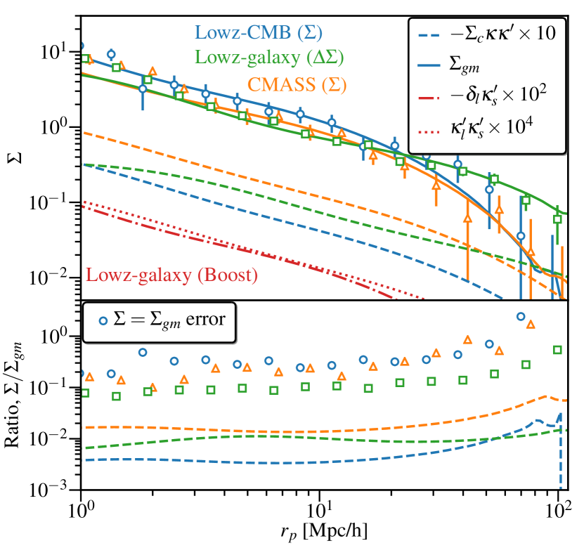
In Fig. 7(b), we show the estimated contamination in lensing measurements using full calculations incorporating lens-source redshift distributions. Magnification contamination introduces a bias of order $\sim 1\%$ in $\Delta\Sigma$. Note that this contamination can increase for high lens redshifts as the $\kappa\kappa$ or $\gamma\kappa$ term becomes larger.

B.2.1 Bias in boost factor

Source galaxies that are physically associated with lens galaxies do not contribute to the lensing shear but do lower the normalization of the lensing measurement around lens galaxies. As described in Section 2.1.1, to account for this effect the final lensing measurement is multiplied by the boost factor, $b_{F}$, defined as

$$b_{F}(r_{p})=\frac{\sum_{ls}w_{ls}(r_{p})}{\sum_{Rs}w_{Rs}(r_{p})}=\frac{1}{N}\int dz_{l}p(z_{l})f_{k}(\chi_{l})^{-2}\int dz_{p}p(z_{p})\Sigma_{c}^{-2}(z_{l},z_{p})\int dz_{s}p(z_{s}|z_{p})(1+\left\langle\delta_{l}\delta_{s}\right\rangle(r_{p}))$$ (58)

where $\Sigma_{c}^{-2}(z_{l},z_{p})$ arises due to lens-source pair weighting, $w_{ls}$. $f_{k}(\chi_{l})^{-2}$ acts as an effective lens weight as the number of source galaxies contributing to a fixed comoving bin decreases with increasing lens redshift (in other words, the comoving projected number density of source galaxies in the lens plane decreases with lens redshift).

However, in the presence of magnification, the number density of source galaxies around lenses changes, modifying the boost factor as

$$\widehat{b}_{F}(r_{p})= \frac{1}{N}\int dz_{l}p(z_{l})f_{k}(\chi_{l})^{-2}\int dz_{p}p(z_{p})\Sigma_{c}^{-2}(z_{l},z_{p})\int dz_{s}p(z_{s}|z_{p})\left[1+\left\langle(\delta_{l}+\kappa^{\prime}_{l})(\delta_{s}+\kappa^{\prime}_{s})\right\rangle(r_{p})\right]$$

$$= b_{F}(r_{p})+\frac{1}{N}\int dz_{l}p(z_{l})f_{k}(\chi_{l})^{-2}\int dz_{p}p(z_{p})\Sigma_{c}^{-2}(z_{l},z_{p})\int dz_{s}p(z_{s}|z_{p})\left[\left\langle\kappa^{\prime}_{l}\delta_{s}+\delta_{l}\kappa^{\prime}_{s}+\kappa^{\prime}_{l}\kappa^{\prime}_{s}\right\rangle(r_{p})\right]$$

$$\approx b_{F}(r_{p})+\frac{1}{N}\int dz_{l}p(z_{l})f_{k}(\chi_{l})^{-2}\int dz_{p}p(z_{p})\Sigma_{c}^{-2}(z_{l},z_{p})\int dz_{s}p(z_{s}|z_{p})\left[\left\langle\delta_{l}\kappa^{\prime}_{s}+\kappa^{\prime}_{l}\kappa^{\prime}_{s}\right\rangle(r_{p})\right]$$ (59)

Here we assume that source galaxies are always behind the lens and hence ignore the $\kappa^{\prime}_{l}\delta_{s}$ term in the last equality. Since the excess galaxies entering (or exiting) the source sample due to magnification do contribute to the lensing shear, the measured boost factor is biased by

$$\frac{{\delta b_{F}}}{b_{F}}(r_{p})=\frac{1}{b_{F}N}\int dz_{l}p(z_{l})f_{k}(\chi_{l})^{-2}\int dz_{p}p(z_{p})\Sigma_{c}^{-2}(z_{l},z_{p})\int dz_{s}p(z_{s}|z_{p})\left[\left\langle\delta_{l}\kappa^{\prime}_{s}+\kappa^{\prime}_{l}\kappa^{\prime}_{s}\right\rangle(r_{p})\right]$$ (60)

$\alpha_{s}\approx 0.55$ for our source sample. The $\delta_{l}\kappa^{\prime}_{s}$ term can be approximated as $2(\alpha_{s}-1)\frac{\Sigma_{gm}}{b_{F}\Sigma_{\text{crit}}}$ in terms of lens $\Sigma_{gm}$. For the lens-source pairs in our analysis, the effective $\Sigma_{\text{crit}}\sim 4600[hM_{\odot}/pc^{2}]$ and thus the contamination from the $\delta_{l}\kappa_{s}^{\prime}$ term is order $10^{-4}\times\Sigma_{gm}$. $\kappa^{\prime}_{l}\kappa^{\prime}_{s}$ is similar to the term derived earlier in the section, except for the $\Sigma_{\text{crit}}$ factor and will be order $10^{-5}$–$10^{-6}$.

B.3 Bias in $E_{G}$

The bias in $E_{G}$ can be estimated as (here we ignore the bias in $f$ as the bias in multipole moments is order 0.1% or lower compared to $\sim 5\%$ or higher uncertainty in $f$)

$$\frac{\Delta E_{G}}{E_{G}}(r_{p})= \frac{\widehat{b}_{F}}{b_{F}}\frac{\widehat{\Delta\Sigma}}{\Delta\Sigma}\frac{w_{gg}}{\widehat{w}_{gg}}(r_{p})-1\approx\frac{\langle\Sigma_{\text{crit}}\gamma_{t}\kappa^{\prime}\rangle}{\Delta\Sigma}+\frac{\left\langle\delta_{l}\kappa^{\prime}_{s}\right\rangle}{b_{F}}+\frac{\left\langle\kappa^{\prime}_{l}\kappa^{\prime}_{s}\right\rangle}{b_{F}}+\frac{w_{g\kappa^{\prime}}}{w_{gg}}-\frac{w_{\kappa^{\prime}\kappa^{\prime}}}{w_{gg}}\approx 10^{-2}$$ (61)

Here for brevity, we omitted showing various integrals involved in the terms. Since the boost factor is multiplied to the lensing signal, it also affects $E_{G}$ as a multiplicative factor. The final corrections applied to the $E_{G}$ measurement are shown in Fig. 5 ($C_{\text{lens}}$), for the case of LOWZ sample.

Appendix C Testing the $E_{G}$ corrections using different mock catalogues

In this section we test the theoretical uncertainties associated with corrections computed from mocks, especially $C_{nl}$, using mock catalogues with different HOD models. For this purpose, we construct light cones from the BigMultiDark Planck simulation (BigMDPL; Klypin et al., 2016) using all the available snapshots in the range $0.16<z<0.36$. This is a simulation of a flat $\Lambda$CDM model, with Planck 2013 cosmological parameters (Planck Collaboration et al., 2014), $\Omega_{m}=0.307$, $\Omega_{\Lambda}=0.693$, $h=0.678$ and $\sigma_{8}=0.829$. The BigMDPL simulation has 3840³ particles with a mass resolution of 2.4$\times 10^{10}$ $h^{-1}M_{\odot}$ and a box size of 2.5 $h^{-1}$Mpc. These features allow the creation of light cones with a volume comparable to BOSS with resolved dark matter halos in the mass range predicted for the LOWZ and CMASS galaxies. Dark matter halos are defined using the Robust Over-density Calculation using K-Space Topologically Adaptive Refinement halo finder (rockstar; Behroozi et al., 2013).

We use the above light cones to produce galaxy mocks that reproduce the clustering at different redshifts and the radial selection function of the observed sample. In order to populate the dark matter halos of the simulation we implement the subhalo abundance matching (SHAM) used by Rodríguez-Torres et al. (2016). The scatter is included using the maximum circular velocity over the whole history of the (sub)halo, $V_{\text{peak}}$, using the relation

$$V_{\text{peak}}^{scat}=(1+\mathcal{G}(0,\sigma_{\textsc{sham}}))V_{\text{peak}},$$ (62)

where $\mathcal{G}$ is a random gaussian number from a distribution with mean 0 and standard deviation $\sigma_{\textsc{ham}}$. We sort all (sub)halos using $V_{\text{peak}}^{scat}$ and select objects from the largest velocity and continuing down until we reach the number density of the observed sample. The scatter between halos and galaxies is fixed using the projected correlation function of the LOWZ data between $2<r_{p}<30$ $h^{-1}$ Mpc for 3 different redshift bins in the range $0.16<z<0.36$.

We do not distinguish between host halos and subhalos in the first light-cone. This produces a LOWZ mock with 12.5% of galaxies living in subhalos. In order to produce a different HOD, we include an additional parameter which models the fraction of galaxies living in subhalos, $f_{sat}$. It will force the model to populate a desired fraction of subhalos with galaxies, rather than the value that naturally arises through the procedure described above. After including the new parameter, we produce 4 different light-cones, first increasing the fraction of satellites by 10 and 15 percent and then decreasing by the same factors. In all cases, we fix the scatter to reproduce the projected correlation function of the LOWZ sample.

In addition to $C_{nl}$ measured using simulations presented in section 3.5, we also compute $C_{nl}$ from one of BigMDPL mocks (labeled as ‘Z Mocks’). We then apply the three sets of $C_{nl}$ to mocks with different HODs to check if we recover $E_{G}$ accurately. In Fig. 9(a), we show the relative bias in the corrected $\left\langle E_{G}\right\rangle$ relative to the theoretical prediction. Applying no corrections, $\left\langle E_{G}\right\rangle$ is biased low by $\sim 3\%$. Applying the correction from same MDPL mocks, we recover the $\left\langle E_{G}\right\rangle$ to within $\lesssim 0.5\%$ independent of the HOD. However, applying the correction from different simulations leads to an overcorrection, and $\left\langle E_{G}\right\rangle$ is biased high. As we show in Fig. 9(b), this is primarily driven by differences in the non-linear physics, which leads to different $C_{nl}$, across different simulations. The corrections used for our main results, from the $z=0.25$ snapshot with the fiducial HOD (no variation in satellite fraction), recovers $\left\langle E_{G}\right\rangle$ to within $\sim 2\%$ for all HODs. Thus we add $2\%$ systematic uncertainty due to these corrections to our results.

(a)

(b)

Figure 9: a) Ratio of theoretical prediction of $E_{G}$  $E_{G,th}$ with $E_{G}$ measured using mocks with different HODs (variable satellite fraction) and different sets of corrections applied. ‘Z mocks’ correction is computed from MDPL mocks with default satellite fraction ($0\%$ variation). b) $C_{nl}$ correction computed from different mocks that are used for corrections in a) (same color scheme in both panels). The differences in the $C_{nl}$ result in variations $\left\langle E_{G}\right\rangle$ at order of $1-2\%$ and thus we add $2\%$ systematic uncertainty resulting from these corrections.

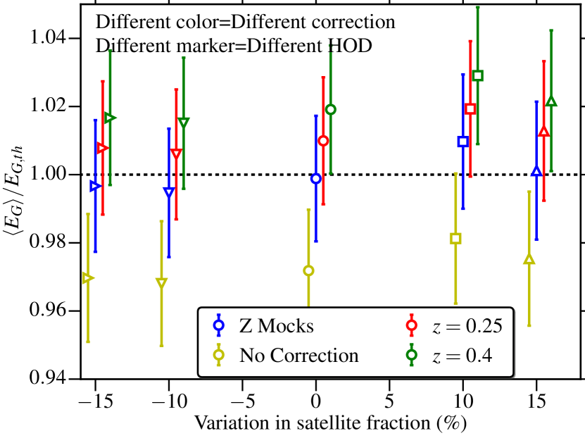
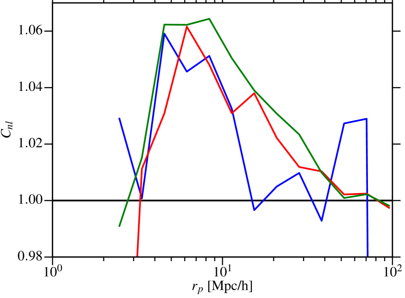
Appendix D Photo-z Lensing bias estimates using clustering redshifts

In this section, we present the estimates of the true redshift distribution $p(z_{s})$ for our photometric source sample, closely following the formalism developed by Ménard et al. (2013); van Daalen & White (2017). We use a random subsample of our source sample containing $\sim 2\times 10^{6}$ galaxies and split it into 40 photo-$z$ bins containing approximately equal numbers of galaxies. These samples are then cross-correlated with the BOSS spectroscopic sample (LOWZ+CMASS), which is split into bins of size $\delta z=0.05$ in the range $z\in[0.1,0.8]$ and two additional bins in the ranges $z\in[0,0.1]$ and $z\in[0.8,1]$. The BOSS sample that we use does not have many galaxies for $z\in[0.8,1]$, where the constraints will be very noisy. We tested our results by omitting this bin and the qualitative trends in the lensing bias presented later in this section do not change, though omitting that bin does change the actual values of the bias in the lensing signal by $\sim 4\%$. This is because the galaxies at these redshifts have low $\Sigma_{\text{crit}}$ and hence have larger weight in the lensing measurement, and $\Sigma_{\text{crit}}$ at larger source redshifts is relatively less affected by small changes in redshifts.

To compute auto- and cross-correlations between the spectroscopic samples, we use the standard Landy-Szalay estimator (Landy & Szalay, 1993), but for cross-correlations involving the source sample we use the sub-optimal estimator as we do not have a good estimate for the on-sky selection function of the source catalog and hence we lack random catalogs for that sample:

$$w_{s_{i}-s_{j}}(\theta)= \frac{\sum_{\theta}(D_{s_{i}}-R_{s_{i}})(D_{s_{j}}-R_{s_{j}})}{\sum_{\theta}R_{s_{i}}R_{s_{j}}}=\frac{\sum_{\theta}(D_{s_{i}}D_{s_{j}}-R_{s_{i}}D_{s_{j}}-D_{s_{i}}R_{s_{j}}+R_{s_{i}}R_{s_{j}})}{\sum_{\theta}R_{s_{i}}R_{s_{j}}}$$ (63)

$$w_{p_{i}-s_{j}}(\theta)= \frac{\sum_{\theta}D_{p_{i}}(D_{s_{j}}-R_{s_{j}})}{\sum_{\theta}D_{p_{i}}R_{s_{j}}}=\frac{\sum_{\theta}(D_{p_{i}}D_{s_{j}}-D_{p_{i}}R_{s_{j}})}{\sum_{\theta}D_{p_{i}}R_{s_{j}}}$$ (64)

Here the subscript ${p_{i}}$ refers to the $i^{th}$ photometric sample, $s_{i}$ refers to the $i^{th}$ spectroscopic sample and $\sum_{\theta}$ indicates that summation is carried over pairs with separation $\theta$ within the limits of the given bin. Then we integrate the correlation functions to obtain

$$W_{a-b}=\int_{\theta_{\text{min}}}^{\theta_{\text{max}}}w_{a-b}(\theta)\mathcal{W}(\theta)\theta d\theta$$ (65)

We use the weight function $\mathcal{W}(\theta)=1/\theta$, as suggested by Ménard et al. (2013). We use $\theta_{\text{min}}=0.03$ degree and $\theta_{\text{max}}=0.5$ degree. These choices are primarily dictated by the noise and systematic bias in the measured cross-correlation functions, which are largely determined by the SDSS number density at small $\theta$ and our use of the sub-optimal estimator at large $\theta$, which increases the variance (Singh et al., 2016a, there is also some evidence of biases due to selection function effects in some bins).

The cross correlation between a photometric sample, $p$, and spectroscopic sample $s_{i}$ can be modeled as

$$W_{p-s_{i}}=\sum_{j=1}^{N_{s}}b_{R,p-s_{j}}f_{p,s_{j}}W_{s_{i}-s_{j}}.$$ (66)

$N_{s}$ is the number of spectroscopic subsamples, $f_{p,s_{j}}\approx p(z_{s})\Delta z_{s}$ is the fraction of the photometric sample within the redshift range of spectroscopic bin $j$ and the bias ratio $b_{R,p-s_{j}}$ is defined as

$$b_{R,p-s_{j}}=\begin{cases}\frac{b_{p,s_{j}}}{b_{s_{j}}}&z_{s_{j}}\leq z_{s_{i}}\\ 1&\text{otherwise}.\end{cases}$$

$b_{p,s_{j}}$ is the (integrated) bias of photometric galaxies that lie in redshift bin $z_{s_{j}}$ and $b_{s_{j}}$ is the bias of spectroscopic galaxies (measured by fitting the linear$+$halofit matter correlation function to $w_{s_{j}-s_{j}}$) in the same bin. If $z_{s_{j}}\leq z_{s_{i}}$, galaxies at $z_{s_{j}}$ are either correlated with galaxies at $z_{s_{i}}$ ($z_{s_{j}}=z_{s_{i}}$) or they are at lower redshift and are lensing the galaxies at higher redshift $z_{s,i}$. When $z_{s_{j}}>z_{s_{i}}$, galaxies at $z_{s_{i}}$ act as lens and hence the correlations depend only on the bias of the spectroscopic galaxies in $z_{s_{i}}$ and the ratio is 1 (this is strictly not true as lensing effects (convergence) also depend on the luminosity function of the source sample as shown in appendix B, but we ignore that effect here). We also stress here that bias going into our estimation is some effective bias integrated over the scales and can also contain effects from non-linear cross correlation coefficients between spectroscopic and photometric samples (similar to $r_{cc}$).

In our fitting procedure, we leave $b_{p,s_{j}}$ as a free parameter, though we do put hard lower and upper limits on the values it can take and also assume that it follows some simple redshift evolution. For hard limits, we use $b_{\text{min}}<b_{p,s_{j}}<3\,\forall\,p,s_{j}$, where the upper limit is fixed to 3 and for the lower limit we try 3 different values $b_{\text{min}}=[0,0.4,0.7]$. $b_{\text{min}}\approx 0.7$ is motivated by the lower limit of halo bias in simulations (e.g., Tinker et al., 2010). However, to accommodate any effects of non-linear physics, we also do the analysis with different lower limits of galaxy bias. To fit for the redshift evolution, we try three different functions: constant, linear and power-law, with two free parameters, $b_{0}$ and $b_{1}$, to be fitted,

$$b_{p}(z)= b_{0}\left(\frac{1+z}{1+\overline{z}_{p}}\right)^{b_{1}}$$ (67)

$$b_{p}(z)= b_{0}\left[{1+b_{1}(z-\overline{z}_{p}})\right]$$ (68)

where $b_{1}=0$ for constant bias and $\overline{z}_{p}$ is the mean photometric redshift of the given photometric subsample.

For each photometric redshift bin, we adopt a Gaussian likelihood as

$$L_{W}=\frac{1}{\sqrt{|\Sigma|}}\exp\left(-\frac{1}{2}(\widehat{W}_{p-s_{i}}-W_{p-s_{i}})^{T}\Sigma^{-1}(\widehat{W}_{p-s_{i}}-W_{p-s_{i}})\right)$$ (69)

We fit for $f_{p,s_{j}},b_{0},$ and $b_{1}$. To fit for the fractional distribution of galaxies, $f_{p,s_{j}}$, we use two separate methods. In the first method, we assume the $p(z_{s})$ is Gaussian and integrate the $p(z_{s})$ within a bin to obtain $f_{p}$. In this case, the fitting parameters are the mean and variance of the Gaussian $p(z_{s})$. However, using a Gaussian function for the $p(z_{s})$ is a simplification that may not be justified in reality. So we also use a non-parametric fitting procedure where each of the $f_{p,s_{j}}$ are free parameters. In this case, we require that $-f_{l}<f_{p,s_{j}}<1+f_{l}$. We test the values $f_{l}=[0,0.05,0.1]$, where values $>0$ are necessary to accommodate shot noise. While the second method is in principle the most general form for $f_{p}$, the results have a higher variance and can be more susceptible to the effects of bias-$f_{p}$ degeneracy. When computing the photo-z bias in lensing, any bins $j$ with best-fitting $f_{p,s_{j}}<0$ are set to zero (since bins with no galaxies due to shot noise will not contribute anything to lensing).

In addition, we also require that the sum of $f_{p,s_{j}}$ ($\sum_{j}f_{p,s_{j}}$) should be close to 1. For this we add an additional term in the likelihood as

$$\mathcal{L}= L_{W}\frac{1}{\sqrt{N_{p,f}}}\exp\left(\frac{-1}{2}\frac{N_{p,f}^{2}(\sum_{j}f_{p,s_{j}}-1)^{2}}{N_{p,f}}\right)$$ (70)

$$N_{p,f}= \frac{500}{\overline{z}_{p}}$$ (71)

Where $N_{p,f}$ should ideally be the number of galaxies in the given photometric sample. However, since the redshift extent of the spectroscopic sample is less than that of the photometric sample, we loosen the likelihood for samples at higher photometric redshift, hence the dependence on $z_{p}$. 500 was chosen so that $500/\text{min}(z_{p})$ is of order 50,000, which is the number of galaxies in each photometric bin.

Once we have the spectroscopic redshift distribution for given photometric samples, we can estimate the bias, $B_{L}$ in measured $\widehat{\Delta\Sigma}$ as (Nakajima et al., 2012) (note that we use different notation than Nakajima et al. (2012) as $b_{z}$ can be confused with redshift-dependent bias)

$$B_{L}=\frac{\widehat{\Delta\Sigma}}{\Delta\Sigma}=\frac{\int dz_{l}\,p(z_{l})D(z_{l})^{2}b(z_{l})f_{k}(\chi_{l})^{-2}\int dz_{p}\,p(z_{p})w_{ls}(z_{l},z_{p})\int dz_{s}\,p(z_{s}|z_{p})\frac{\Sigma_{\text{crit}}(z_{l},z_{p})}{\Sigma_{\text{crit}}(z_{l},z_{s})}}{\int dz_{l}\,p(z_{l})D(z_{l})^{2}b(z_{l})f_{k}(\chi_{l})^{-2}\int dz_{p}\,p(z_{p})w_{ls}(z_{l},z_{p})\int dz_{s}\,p(z_{s}|z_{p})}$$ (72)

$z_{l}$ is the lens redshift, $z_{p}$ is the photometric redshift, $z_{s}$ is the true source redshift and $\int dz_{s}\,p(z_{s}|z_{p})=f_{p,s}$. $D(z_{l})$ is the growth function at lens redshift, $b(z_{l})$ is the galaxy bias, $f_{k}(\chi_{l})$ is the comoving transverse distance at lens redshift (accounts for the fact that effective number of source galaxies entering a fixed comoving distance bin decreases at higher lens redshift – Nakajima et al. 2012) and $w_{ls}$ is the weight as described in Eq. (9). For our computation, we assume that the clustering of lens galaxies is redshift independent and hence $b(z_{l})\propto D(z_{l})^{-1}$ and $\Delta\Sigma(z_{l})\propto D(z_{l})$.

In Fig. 10, we show the redshift distribution (fraction of galaxies in each bin) estimated assuming a Gaussian model for $p(z_{s})$ (blue points) and when using the non-parametric $f_{p}$ model (red points). We also show the $f_{p}$ obtained using a representative calibration sample with spectroscopic redshifts from Nakajima et al. (2012). $f_{p}$ obtained using the Gaussian model is less noisy, but for any given photometric sample, the bins in true redshift are strongly correlated. In the case where the $f_{p}$ are treated as independent parameters, the correlations across bins are not significant and the distributions appear to capture more features, though to some extent this can be caused by noise in clustering measurements and the degeneracies with the galaxy bias.

In Fig. 11 we show the bias in the galaxy-galaxy lensing measurement due to photometric redshift bias and scatter, calculated using the redshift distributions estimated from the clustering analysis. We show the estimates using different bias and $f_{p}$ models along with different priors on the galaxy bias and $f_{p}$. Our results are not very sensitive to the bias evolution models, likely due to the relatively narrow redshift bins. However, in the case where the $f_{p}$ values are treated as free parameters, the results are sensitive to the priors on $f_{p}$ and the bias, especially the lower limit on bias. This is primarily caused by the degeneracy between the bias and $f_{p}$, along with the noise in the correlation function measurements that makes it difficult to infer so many free parameters. We attempt to overcome this difficulty using the Gaussian $p(z_{s})$. The results in this case are less sensitive to priors on galaxy bias. However, the $S/N$ in the estimate of the lensing bias is not improved by much, which suggests that we do not gain much more information by constraining $p(z_{s})$ (the $f(z_{s})$ obtained in this case are correlated across bins). As a result we do not attempt to use more complicated functions than gaussian which may capture more features of $p(z_{s})$.

For the physically-motivated choice of priors, $b_{\text{min}}\in[0.4,0.7]$ and $f_{l}\in[0.05,0.1]$, our results are consistent (within $\lesssim 5\%$) with the bias in the lensing signal estimated using the representative spectroscopic calibration sample. This value has been used in this and previous works to correct the lensing measurements for the impact of photo-$z$ bias and scatter.

Our results suggest that more work is required to carefully choose the priors and functional forms for $f_{p}$ to further develop the clustering redshift method (as used in this work) for calibration of the galaxy-galaxy lensing signal. However, our results demonstrate that the bias in our galaxy-galaxy lensing signals due to photometric redshift bias and scatter is well constrained at the $\lesssim 5\%$ level and hence is not likely the full explanation for $\sim 15\%$ discrepancy observed between the $E_{G}$ measurements and the prediction from the Planck $\Lambda\text{CDM}$ model.

Figure 10: Redshift distribution estimates $f(z)$ for different photometric redshift bins, where each panel represents a given photo-z selected sample. Red and orange points are for the fits with $f(z)$ in each bin as a free parameter and assuming a Gaussian redshift distribution, respectively. For both red and orange curves in this plot we use $b_{\text{min}}=0.7$; for the red points, $f_{l}=0.05$. The blue curves show the $f(z)$ obtained using spectroscopic redshifts from the representative calibration sample.

(a) Non-Parametric $p(z)$

(b) Gaussian $p(z)$

Figure 11: a) Probability distribution of bias in the lensing signal, $B_{L}$, due to photometric redshifts, for different choices of lower limit on bias and redshift fraction. The vertical dashed black lines show the estimate using spectroscopic redshifts in the representative calibration sample. The blue lines/points are assuming power law model for the bias-redshift relation, orange color is for linear model while green is for constant bias with redshift. When bias is allowed to evolve with redshift, there is strong dependence of the inferred bias on the lensing signal on the priors chosen, though the choice of model for the bias-redshift relation does not affect it too strongly. In all cases, the difference between the lensing bias from the clustering redshift method and that derived using spectroscopic redshifts ($\sim 0.92$) is $\lesssim 10\%$. b) Same as a), using gaussian model for $p(z)$. Green curves show the estimate when we assume galaxy bias to be constant with redshift ($b_{1}=0$ in Eq. (67)).

References

- Abazajian et al. (2009) Abazajian K. N., et al., 2009, ApJS, 182, 543
- Ahn et al. (2012) Ahn C. P., et al., 2012, ApJS, 203, 21
- Aihara et al. (2011) Aihara H., et al., 2011, ApJS, 193, 29
- Alam et al. (2015a) Alam S., et al., 2015a, ApJS, 219, 12
- Alam et al. (2015b) Alam S., Ho S., Vargas-Magaña M., Schneider D. P., 2015b, MNRAS, 453, 1754
- Alam et al. (2016a) Alam S., et al., 2016a, preprint, (arXiv:1607.03155)
- Alam et al. (2016b) Alam S., Ho S., Silvestri A., 2016b, MNRAS, 456, 3743
- Alam et al. (2017a) Alam S., Miyatake H., More S., Ho S., Mandelbaum R., 2017a, MNRAS, 465, 4853
- Alam et al. (2017b) Alam S., Zhu H., Croft R. A. C., Ho S., Giusarma E., Schneider D. P., 2017b, MNRAS, 470, 2822
- Alam et al. (2017c) Alam S., Croft R. A. C., Ho S., Zhu H., Giusarma E., 2017c, MNRAS, 471, 2077
- Amon et al. (2018) Amon A., et al., 2018, MNRAS, 479, 3422
- Anderson et al. (2014) Anderson L., et al., 2014, MNRAS, 441, 24
- Baldauf et al. (2010) Baldauf T., Smith R. E., Seljak U., Mandelbaum R., 2010, Phys.Rev.D, 81, 063531
- Bartelmann & Schneider (2001) Bartelmann M., Schneider P., 2001, Phys.Rep., 340, 291
- Behroozi et al. (2013) Behroozi P. S., Wechsler R. H., Wu H.-Y., 2013, ApJ, 762, 109
- Bernardeau et al. (2002) Bernardeau F., Colombi S., Gaztañaga E., Scoccimarro R., 2002, Phys.Rep., 367, 1
- Bernstein (2009) Bernstein G. M., 2009, ApJ, 695, 652
- Bernstein & Jarvis (2002) Bernstein G. M., Jarvis M., 2002, AJ, 123, 583
- Betoule et al. (2014) Betoule M., et al., 2014, A&A, 568, A22
- Beutler et al. (2012) Beutler F., et al., 2012, MNRAS, 423, 3430
- Beutler et al. (2016) Beutler F., et al., 2016, preprint, (arXiv:1607.03150)
- Blake et al. (2016) Blake C., et al., 2016, MNRAS, 456, 2806
- Blanton et al. (2003) Blanton M. R., Lin H., Lupton R. H., Maley F. M., Young N., Zehavi I., Loveday J., 2003, AJ, 125, 2276
- Blazek et al. (2012) Blazek J., Mandelbaum R., Seljak U., Nakajima R., 2012, J. Cosmology Astropart. Phys., 5, 41
- Bolton et al. (2012) Bolton A. S., et al., 2012, AJ, 144, 144
- Cappi (1995) Cappi A., 1995, A&A, 301, 6
- Carlson et al. (2013) Carlson J., Reid B., White M., 2013, MNRAS, 429, 1674
- Chan et al. (2012) Chan K. C., Scoccimarro R., Sheth R. K., 2012, Phys.Rev.D, 85, 083509
- Crocce & Scoccimarro (2006) Crocce M., Scoccimarro R., 2006, Phys.Rev.D, 73, 063519
- Crocce et al. (2012) Crocce M., Scoccimarro R., Bernardeau F., 2012, MNRAS, 427, 2537
- DES Collaboration et al. (2017) DES Collaboration et al., 2017, preprint, (arXiv:1708.01530)
- Dawson et al. (2013) Dawson K. S., et al., 2013, AJ, 145, 10
- Eisenstein et al. (2001) Eisenstein D. J., et al., 2001, AJ, 122, 2267
- Feldmann et al. (2006) Feldmann R., et al., 2006, MNRAS, 372, 565
- Giannantonio et al. (2016) Giannantonio T., et al., 2016, MNRAS, 456, 3213
- Gil-Marín et al. (2016) Gil-Marín H., et al., 2016, MNRAS, 460, 4188
- Górski et al. (2005) Górski K. M., Hivon E., Banday A. J., Wandelt B. D., Hansen F. K., Reinecke M., Bartelmann M., 2005, ApJ, 622, 759
- Grieb et al. (2016) Grieb J. N., et al., 2016, preprint, (arXiv:1607.03143)
- Gunn et al. (1998) Gunn J. E., et al., 1998, AJ, 116, 3040
- Gunn et al. (2006) Gunn J. E., et al., 2006, AJ, 131, 2332
- Hamilton (1992) Hamilton A. J. S., 1992, ApJ, 385, L5
- Hamilton (1997) Hamilton A. J. S., 1997, MNRAS, 289, 285
- Hand et al. (2017) Hand N., Seljak U., Beutler F., Vlah Z., 2017, J. Cosmology Astropart. Phys., 10, 009
- Hartlap et al. (2007) Hartlap J., Simon P., Schneider P., 2007, A&A, 464, 399
- Heymans et al. (2013) Heymans C., et al., 2013, MNRAS, 432, 2433
- Hildebrandt et al. (2009) Hildebrandt H., van Waerbeke L., Erben T., 2009, A&A, 507, 683
- Hildebrandt et al. (2016) Hildebrandt H., et al., 2016, preprint, (arXiv:1606.05338)
- Hirata & Seljak (2003) Hirata C., Seljak U., 2003, MNRAS, 343, 459
- Hirata et al. (2008) Hirata C. M., Ho S., Padmanabhan N., Seljak U., Bahcall N. A., 2008, Phys.Rev.D, 78, 043520
- Hu & White (2001) Hu W., White M., 2001, ApJ, 554, 67
- Jain & Khoury (2010) Jain B., Khoury J., 2010, Annals of Physics, 325, 1479
- Jennings et al. (2011) Jennings E., Baugh C. M., Pascoli S., 2011, ApJ, 727, L9
- Joudaki et al. (2017) Joudaki S., et al., 2017, MNRAS, 465, 2033
- Kaiser (1987) Kaiser N., 1987, MNRAS, 227, 1
- Kaiser et al. (1995) Kaiser N., Squires G., Broadhurst T., 1995, ApJ, 449, 460
- Kilbinger (2015) Kilbinger M., 2015, Reports on Progress in Physics, 78, 086901
- Kilbinger et al. (2013) Kilbinger M., et al., 2013, MNRAS, 430, 2200
- Klypin et al. (2016) Klypin A., Yepes G., Gottlöber S., Prada F., Heß S., 2016, MNRAS, 457, 4340
- Komatsu et al. (2011) Komatsu E., et al., 2011, ApJS, 192, 18
- Landy & Szalay (1993) Landy S. D., Szalay A. S., 1993, ApJ, 412, 64
- Leauthaud et al. (2017) Leauthaud A., et al., 2017, MNRAS, 467, 3024
- Leonard et al. (2015) Leonard C. D., Ferreira P. G., Heymans C., 2015, J. Cosmology Astropart. Phys., 12, 051
- Lewis & Bridle (2002a) Lewis A., Bridle S., 2002a, Phys.Rev.D, 66, 103511
- Lewis & Bridle (2002b) Lewis A., Bridle S., 2002b, Phys. Rev., D66, 103511
- Lewis & Challinor (2006) Lewis A., Challinor A., 2006, Phys.Rep., 429, 1
- Mandelbaum (2017) Mandelbaum R., 2017, preprint, (arXiv:1710.03235)
- Mandelbaum et al. (2005) Mandelbaum R., et al., 2005, MNRAS, 361, 1287
- Mandelbaum et al. (2011) Mandelbaum R., et al., 2011, MNRAS, 410, 844
- Mandelbaum et al. (2012) Mandelbaum R., Hirata C. M., Leauthaud A., Massey R. J., Rhodes J., 2012, MNRAS, 420, 1518
- Mandelbaum et al. (2013) Mandelbaum R., Slosar A., Baldauf T., Seljak U., Hirata C. M., Nakajima R., Reyes R., Smith R. E., 2013, MNRAS, 432, 1544
- Mandelbaum et al. (2017) Mandelbaum R., et al., 2017, preprint, (arXiv:1710.00885)
- Manera et al. (2015) Manera M., et al., 2015, MNRAS, 447, 437
- Massey et al. (2007) Massey R., et al., 2007, ApJS, 172, 239
- Ménard et al. (2013) Ménard B., Scranton R., Schmidt S., Morrison C., Jeong D., Budavari T., Rahman M., 2013, preprint, (arXiv:1303.4722)
- Moradinezhad Dizgah & Durrer (2016) Moradinezhad Dizgah A., Durrer R., 2016, J. Cosmology Astropart. Phys., 9, 035
- Nakajima et al. (2012) Nakajima R., Mandelbaum R., Seljak U., Cohn J. D., Reyes R., Cool R., 2012, MNRAS, 420, 3240
- Padmanabhan et al. (2008) Padmanabhan N., et al., 2008, ApJ, 674, 1217
- Perlmutter et al. (1999) Perlmutter S., et al., 1999, ApJ, 517, 565
- Planck Collaboration et al. (2014) Planck Collaboration et al., 2014, A&A, 571, A16
- Planck Collaboration et al. (2015a) Planck Collaboration et al., 2015a, preprint, (arXiv:1502.01589)
- Planck Collaboration et al. (2015b) Planck Collaboration et al., 2015b, preprint, (arXiv:1502.01591)
- Pourtsidou (2016) Pourtsidou A., 2016, MNRAS, 461, 1457
- Pullen et al. (2015) Pullen A. R., Alam S., Ho S., 2015, MNRAS, 449, 4326
- Pullen et al. (2016) Pullen A. R., Alam S., He S., Ho S., 2016, MNRAS, 460, 4098
- Reid & Spergel (2009) Reid B. A., Spergel D. N., 2009, ApJ, 698, 143
- Reid et al. (2012) Reid B. A., et al., 2012, MNRAS, 426, 2719
- Reid et al. (2014a) Reid B. A., Seo H.-J., Leauthaud A., Tinker J. L., White M., 2014a, MNRAS, 444, 476
- Reid et al. (2014b) Reid B. A., Seo H.-J., Leauthaud A., Tinker J. L., White M., 2014b, MNRAS, 444, 476
- Reid et al. (2016) Reid B., et al., 2016, MNRAS, 455, 1553
- Reyes et al. (2010) Reyes R., Mandelbaum R., Seljak U., Baldauf T., Gunn J. E., Lombriser L., Smith R. E., 2010, Nature, 464, 256
- Reyes et al. (2012) Reyes R., Mandelbaum R., Gunn J. E., Nakajima R., Seljak U., Hirata C. M., 2012, MNRAS, 425, 2610
- Richards et al. (2002) Richards G. T., et al., 2002, AJ, 123, 2945
- Riess et al. (1998) Riess A. G., et al., 1998, AJ, 116, 1009
- Riess et al. (2016) Riess A. G., et al., 2016, ApJ, 826, 56
- Rodríguez-Torres et al. (2016) Rodríguez-Torres S. A., et al., 2016, MNRAS,
- Ross et al. (2012) Ross A. J., et al., 2012, MNRAS, 424, 564
- Samushia et al. (2014) Samushia L., et al., 2014, MNRAS, 439, 3504
- Sánchez et al. (2014) Sánchez A. G., et al., 2014, MNRAS, 440, 2692
- Sanchez et al. (2016) Sanchez A. G., et al., 2016, preprint, (arXiv:1607.03147)
- Satpathy et al. (2016) Satpathy S., et al., 2016, preprint, (arXiv:1607.03148)
- Schaan et al. (2016) Schaan E., Krause E., Eifler T., Doré O., Miyatake H., Rhodes J., Spergel D. N., 2016, preprint, (arXiv:1607.01761)
- Schlegel et al. (1998) Schlegel D. J., Finkbeiner D. P., Davis M., 1998, ApJ, 500, 525
- Sheldon et al. (2004) Sheldon E. S., et al., 2004, AJ, 127, 2544
- Sheth & Tormen (1999) Sheth R. K., Tormen G., 1999, MNRAS, 308, 119
- Simpson et al. (2013) Simpson F., et al., 2013, MNRAS, 429, 2249
- Singh et al. (2016b) Singh S., Mandelbaum R., Brownstein J. R., 2016b, preprint, (arXiv:1606.08841)
- Singh et al. (2016a) Singh S., Mandelbaum R., Seljak U., Slosar A., Vazquez Gonzalez J., 2016a, preprint, (arXiv:1611.00752)
- Smee et al. (2013) Smee S. A., et al., 2013, AJ, 146, 32
- Smith et al. (2003) Smith R. E., et al., 2003, MNRAS, 341, 1311
- Song et al. (2018) Song Y.-S., Zheng Y., Taruya A., Oh M., 2018, preprint, (arXiv:1801.04950)
- Steigman (2010) Steigman G., 2010, preprint, (arXiv:1008.4765)
- Stoughton et al. (2002) Stoughton C., et al., 2002, AJ, 123, 485
- Strauss et al. (2002) Strauss M. A., et al., 2002, AJ, 124, 1810
- Takahashi et al. (2012) Takahashi R., Sato M., Nishimichi T., Taruya A., Oguri M., 2012, ApJ, 761, 152
- Taylor et al. (2013) Taylor A., Joachimi B., Kitching T., 2013, MNRAS, 432, 1928
- Tinker et al. (2010) Tinker J. L., Robertson B. E., Kravtsov A. V., Klypin A., Warren M. S., Yepes G., Gottlöber S., 2010, ApJ, 724, 878
- Wang et al. (2014) Wang L., Reid B., White M., 2014, MNRAS, 437, 588
- Weinberg et al. (2013) Weinberg D. H., Mortonson M. J., Eisenstein D. J., Hirata C., Riess A. G., Rozo E., 2013, Phys.Rep., 530, 87
- White (2014) White M., 2014, MNRAS, 439, 3630
- Will (2014) Will C. M., 2014, Living Reviews in Relativity, 17
- Yoo (2009) Yoo J., 2009, Phys.Rev.D, 79, 023517
- Yoo et al. (2009) Yoo J., Fitzpatrick A. L., Zaldarriaga M., 2009, Phys.Rev.D, 80, 083514
- York et al. (2000) York D. G., et al., 2000, AJ, 120, 1579
- Zaldarriaga & Seljak (1999) Zaldarriaga M., Seljak U., 1999, Phys.Rev.D, 59, 123507
- Zhang et al. (2007) Zhang P., Liguori M., Bean R., Dodelson S., 2007, Physical Review Letters, 99, 141302
- Zheng et al. (2005) Zheng Z., et al., 2005, ApJ, 633, 791
- de la Torre et al. (2013) de la Torre S., et al., 2013, A&A, 557, A54
- de la Torre et al. (2016) de la Torre S., et al., 2016, preprint, (arXiv:1612.05647)
- van Daalen & White (2017) van Daalen M. P., White M., 2017, preprint, (arXiv:1703.05326)
- van Uitert et al. (2017) van Uitert E., et al., 2017, preprint, (arXiv:1706.05004)