High order Bellman equations and weakly chained diagonally dominant tensors

Abstract

We introduce high order Bellman equations, extending classical Bellman equations to the tensor setting. We introduce weakly chained diagonally dominant (w.c.d.d.) tensors and show that a sufficient condition for the existence and uniqueness of a positive solution to a high order Bellman equation is that the tensors appearing in the equation are w.c.d.d. M-tensors. In this case, we give a policy iteration algorithm to compute this solution. We also prove that a weakly diagonally dominant Z-tensor with nonnegative diagonals is a strong M-tensor if and only if it is w.c.d.d. This last point is analogous to a corresponding result in the matrix setting and tightens a result from [L. Zhang, L. Qi, and G. Zhou. “M-tensors and some applications.” SIAM Journal on Matrix Analysis and Applications (2014)]. We apply our results to obtain a provably convergent numerical scheme for an optimal control problem using an “optimize then discretize” approach which outperforms (in both computation time and accuracy) a classical “discretize then optimize” approach. To the best of our knowledge, a link between M-tensors and optimal control has not been previously established.

1 Introduction

In this work, we introduce and study the nonlinear problem

$$\text{find }u\in\mathbb{R}^{n}\text{ such that }\min_{P\in\mathcal{P}}\left\{A(P)u^{m-1}-b(P)\right\}=0$$ (1)

where $A(P)$ is an $m$-order and $n$-dimensional real tensor, $b(P)$ is a real vector, $\mathcal{P}$ is a nonempty compact set, and the minimum is taken with respect to the coordinatewise order on $\mathbb{R}^{n}$ (see (iii) in Section 5).

If $m=2$, then $A(P)$ is a square matrix and $A(P)u^{m-1}\equiv A(P)u$ is the ordinary matrix-vector product. In this case, (1) is the celebrated Bellman equation for optimal decision making on a Markov chain. Aside from Markov chains, (1) also arises from discretizations of differential equations from optimal control [14].

If $m>2$, then $A(P)u^{m-1}$ defines a vector whose $i$-th component is a multivariate polynomial in the entries of $u$:

$$(A(P)u^{m-1})_{i}=\sum_{i_{2},\ldots,i_{m}}(A(P))_{ii_{2}\cdots i_{m}}u_{i_{2}}\cdots u_{i_{m}}$$

(see also (2)). As such, we refer to (1) as a Bellman equation of order $m$. We are motivated to study this equation since, as we will see in the sequel, it arises from a so-called “optimize then discretize” [4] scheme for a differential equation.

Our main goal is to characterize the existence and uniqueness of a solution $u$ to (1) and to obtain a fast and provably convergent algorithm for computing it. If $m=2$, existence and uniqueness is guaranteed when $A(P)$ is a nonsingular M-matrix for each $P$ [5, Theorem 2.1] (along with some other mild conditions on the functions $A$ and $b$). We obtain an analogous result for the $m>2$ case when $A(P)$ is a strictly diagonally dominant (and hence nonsingular) M-tensor for each $P$ (Lemma 23 and Lemma 24). M-tensors, a generalization of M-matrices, were introduced in [20, 9] in order to test the positive definiteness of multivariate polynomials.

However, strict diagonal dominance is a rather strong condition. In order to generalize our results, we extend the notion of weakly chained diagonal dominance from matrices to tensors (Definition 15). By restricting our attention to the case in which $\mathcal{P}$ is finite, we establish existence and uniqueness of a solution $u$ to (1) under the weaker requirement that $A(P)$ is a weakly chained diagonally dominant M-tensor (Lemma 26) and give a policy iteration algorithm to compute the solution (Algorithm 1). Analogously to the $m=2$ case, the assumed finitude of $\mathcal{P}$ is sufficient for practical applications, though whether this assumption can be dropped remains an interesting open theoretical question (Remark 27).

We also establish the following result, which should be of broader interest to the M-tensor community:

Theorem 1.

Let $A$ be a weakly diagonally dominant Z-tensor with nonnegative diagonals. Then, the following are equivalent:

1. $A$ is a strong M-tensor.

2. Zero is not an eigenvalue of $A$.

3. $A$ is weakly chained diagonally dominant (Definition 15).

An analogous equivalence result for matrices was recently proved in [1]. Since a weakly irreducibly diagonally dominant tensor is a weakly chained diagonally dominant tensor (Lemma 17), the following is an immediate consequence:

Corollary 2.

Let $A$ be a Z-tensor with nonnegative diagonals. If $A$ is weakly irreducibly diagonally dominant, then $A$ is a strong M-tensor.

Since an irreducible tensor is weakly irreducible (Corollary 10), Theorem 1 and Corollary 2 can be thought of as tightening the following result:

Proposition 3 ([20, Theorem 3.15]).

Let $A$ be a Z-tensor with nonnegative diagonals. If $A$ is strictly or irreducibly diagonally dominant, then $A$ is a strong M-tensor.

Moreover, Theorem 1 yields a graph-theoretic characterization of weakly diagonally dominant strong M-tensors and a fast algorithm to determine if an arbitrary weakly diagonally dominant tensor is a strong M-tensor (Remark 16).

This work is organized as follows. In Section 2, we recall some standard definitions and results for tensors. In Section 3, we introduce the notion of a weakly chained diagonally dominant tensor. A proof of Theorem 1 is given in Section 4. In Section 5, we study high order ($m>2$) Bellman equations. In Section 6, we use our results to study numerically some problems from optimal stochastic control.

2 Preliminaries

For the convenience of the reader, we gather in this section some definitions and well-known results (cf. [17]) concerning tensors of the form

$$A=(a_{i_{1}\cdots i_{m}}),\qquad a_{i_{1}\cdots i_{m}}\in\mathbb{R},\qquad 1\leqslant i_{1},\ldots,i_{m}\leqslant n.$$

Such tensors are called $m$-order and $n$-dimensional real tensors, though we will simply refer to them as “tensors” in this work. We call $a_{1\cdots 1}$, $a_{2\cdots 2}$, etc. the diagonal entries of $A$. All other entries are referred to as off-diagonal.

Definition 4 ([16]).

Let $x=(x_{1},\ldots,x_{n})$ be a vector in $\mathbb{C}^{n}$ and $A=(a_{i_{1}\cdots i_{m}})$ be a tensor. We denote by $x^{[\alpha]}=(x_{1}^{\alpha},\ldots,x_{n}^{\alpha})$ the coordinatewise power of $x$ and by $Ax^{m-1}$ the vector in $\mathbb{C}^{n}$ whose $i$-th entry is

$$\sum_{i_{2},\ldots,i_{m}}a_{ii_{2}\cdots i_{m}}x_{i_{2}}\cdots x_{i_{m}}.$$ (2)

We call $\lambda$ in $\mathbb{C}$ an eigenvalue of $A$ if we can find a vector $x$ in $\mathbb{C}^{n}\setminus\{0\}$ such that

$$Ax^{m-1}=\lambda x^{[m-1]}.$$

The vector $x$ is called an eigenvector associated with $\lambda$. The spectrum $\sigma(A)$ of $A$ is the set of all eigenvalues of $A$. The spectral radius of $A$ is $\rho(A)=\max_{\lambda\in\sigma(A)}|\lambda|$.

Z and M-tensors, defined below, are natural extensions of Z and M-matrices.

Definition 5 ([20, Pg. 440]).

A Z-tensor is a real tensor whose off-diagonal entries are nonpositive.

Definition 6 ([20, Definition 3.1]).

A tensor $A$ is an M-tensor if there exists a nonnegative tensor $B$ (i.e., a tensor with nonnegative entries) and a real number $s\geqslant\rho(B)$ such that

$$A=sI-B$$

where $I$ is the identity tensor (i.e., the tensor with ones on its diagonal and zeros elsewhere). If $s>\rho(B)$, then $A$ is called a strong M-tensor.

Unlike the matrix setting, there are two distinct notions of irreducibility for tensors, introduced in [12]. Both are given below.

Definition 7 ([12, Pg. 739]).

A tensor $A=(a_{i_{1}\cdots i_{m}})$ is reducible if there exists a nonempty proper index subset $\Lambda\subsetneq\{1,\ldots,n\}$ such that

$$a_{ii_{2}\cdots i_{m}}=0\qquad\text{if }i\in\Lambda\text{ and }i_{2},\ldots,i_{m}\notin\Lambda.$$

Otherwise, we say $A$ is irreducible.

Definition 8 ([13, Definition 2.2]).

Let $A=(a_{i_{1}\cdots i_{m}})$ be a tensor and $R(|A|)$, the representation of $A$, denote the $n\times n$ matrix whose $(i,j)$-th entry is given by

$$\sum_{i_{2},\ldots,i_{m}}\left|a_{ii_{2}\cdots i_{m}}\right|\boldsymbol{1}_{\{i_{2},\ldots,i_{m}\}}(j)$$

where $\boldsymbol{1}_{\mathcal{U}}$ is the indicator function of the set $\mathcal{U}$. We say $A$ is weakly reducible if $R(|A|)$ is a reducible matrix. Otherwise, we say $A$ is weakly irreducible.

In [12, Lemma 3.1], the authors show that irreducibility is a stronger requirement than weak irreducibility. We summarize this below, including what we believe to be a simpler proof for the reader’s convenience.

Proposition 9.

A tensor that is weakly reducible is reducible.

Proof.

Let $A=(a_{i_{1}\cdots i_{m}})$ be a weakly reducible tensor so that the $n\times n$ matrix $R(|A|)=(r_{ij})$ is reducible. Then, there exists a nonempty proper index subset $\Lambda\subsetneq\{1,\ldots,n\}$ such that

$$r_{ij}=\sum_{i_{2},\ldots,i_{m}}\left|a_{ii_{2}\cdots i_{m}}\right|\boldsymbol{1}_{\{i_{2},\ldots,i_{m}\}}(j)=0\qquad\text{if }i\in\Lambda\text{ and }j\notin\Lambda.$$

Therefore,

$$a_{ii_{2}\cdots i_{m}}=0\qquad\text{if }i\in\Lambda\text{ and }i_{k}\notin\Lambda\text{ for some }2\leqslant k\leqslant m$$

and hence $A$ is reducible. ∎

Corollary 10.

An irreducible tensor is weakly irreducible.

We close this section with the notion of diagonal dominance.

Definition 11 ([20, Definition 3.14]).

Let $A=(a_{i_{1}\cdots i_{m}})$ be a tensor. We say that the $i$-th row of $A$ is strictly diagonally dominant (s.d.d.) if

$$\left|a_{i\cdots i}\right|>\sum_{(i_{2},\ldots i_{m})\neq(i,\ldots,i)}\left|a_{ii_{2}\cdots i_{m}}\right|.$$ (3)

We say $A$ is s.d.d. if all of its rows are s.d.d. Weakly diagonally dominant (w.d.d.) is defined with weak inequality ($\geqslant$) instead. We use

$$J(A)=\left\{1\leqslant i\leqslant n\colon i\text{ satisfies }\eqref{eq:sdd}\right\}$$

to denote the set of s.d.d. rows of $A$.

Definition 12 ([20, Definition 3.14]).

We say a tensor $A$ is (weakly) irreducibly diagonally dominant if it is (weakly) irreducible, w.d.d., and $J(A)$ is nonempty.

3 Weakly chained diagonally dominant tensors

Before we introduce the notion of weakly chained diagonally dominant (w.c.d.d.) tensors, we define the directed graph associated with a tensor.

Definition 13.

Let $A=(a_{i_{1}\cdots i_{m}})$ be a tensor.

1. The directed graph of $A$, denoted $\operatorname{graph}A$, is a tuple $(V,E)$ consisting of the vertex set $V=\{1,\ldots,n\}$ and edge set $E\subset V\times V$ satisfying $(i,j)\in E$ if and only if $a_{ii_{2}\cdots i_{m}}\neq 0$ for some $(i_{2},\ldots,i_{m})$ such that $j\in\{i_{2},\ldots,i_{m}\}$.

2. A walk in $\operatorname{graph}A$ is a nonempty finite sequence $(i^{1},i^{2}),(i^{2},i^{3}),\ldots,(i^{k-1},i^{k})$ of “adjacent” edges in $E$.

The proof of the next result, being a trivial consequence of the above definition, is omitted.

Lemma 14.

$\operatorname{graph}A=\operatorname{graph}R(|A|)$ for any tensor $A$.

Since each vertex in the directed graph of a tensor corresponds to a row $i$, we use the terms row and vertex interchangeably. To simplify matters, we hereafter denote edges by $i\rightarrow j$ instead of $(i,j)$ and walks by $i^{1}\rightarrow i^{2}\rightarrow\cdots\rightarrow i^{k}$ instead of $(i^{1},i^{2}),\ldots,(i^{k-1},i^{k})$. We are now ready to define w.c.d.d.

Definition 15.

A tensor $A$ is w.c.d.d. if all of the following are satisfied:

1. $A$ is w.d.d.

2. $J(A)$ is nonempty.

3. For each $i^{1}\notin J(A)$, there exists a walk $i^{1}\rightarrow i^{2}\rightarrow\cdots\rightarrow i^{k}$ in $\operatorname{graph}A$ such that $i^{k}\in J(A)$.

If the tensor is of order $m=2$ (i.e., the tensor is a matrix), then the above becomes the usual definition of w.c.d.d. for matrices [1, Definition 2.20].

Remark 16.

A trivial extension of the algorithm in [1] allows us to test if a weakly diagonally dominant tensor is weakly chained diagonally dominant with $O(n^{m})$ effort if the tensor is dense. Less computational effort is required if the tensor is sparse (we refer to [1] for details).

Lemma 17.

A weakly irreducibly diagonally dominant tensor is a w.c.d.d. tensor.

Proof.

If $A$ is weakly irreducibly diagonally dominant, then $J(A)$ is nonempty and $\operatorname{graph}R(|A|)$ is strongly connected (i.e., for any pair of vertices $(i,j)$, there is a walk starting at $i$ and ending at $j$). The result then follows by Lemma 14. ∎

4 Proof of Theorem 1

In the following, we denote by $\operatorname{Re}z$ the real part of a complex number $z$. We say a vector is positive if it lies in the positive orthant $\mathbb{R}_{++}^{n}=(0,\infty)^{n}$. Similarly, any element of $\mathbb{R}_{+}^{n}=[0,\infty)^{n}$ is called a nonnegative vector. Our proof relies on the following results:

Proposition 18 ([20, Theorem 3.3]).

$\min_{\lambda\in\sigma(A)}\operatorname{Re}\lambda$ is nonnegative (resp. positive) whenever $A$ is an M-tensor (resp. strong M-tensor).

Proposition 19 ([20, Theorem 3.15]).

If $A$ is a w.d.d. Z-tensor with nonnegative diagonals, then $A$ is an M-tensor.

Our proof also relies on a corollary to the following result:

Proposition 20 ([10, Pg. 697]).

Let $A$ be a strong M-tensor. For each positive vector $b$ (of compatible size), there exists a unique positive vector $x$ which solves the tensor equation $Ax^{m-1}=b$. Denoting by $A_{++}^{-1}:\mathbb{R}_{++}^{n}\rightarrow\mathbb{R}_{++}^{n}$ the mapping from positive right hand sides $b$ to positive solutions $x$, $A_{++}^{-1}$ is nondecreasing with respect to the coordinatewise order.

The corollary, which is of independent interest, establishes existence (but not uniqueness) of nonnegative solution $x$ to the tensor equation $Ax^{m-1}=b$ when $b$ is a nonnegative vector and $A$ is a strong M-tensor.

Corollary 21.

Let $A$ be a strong M-tensor. Then, there exists a nondecreasing map $A_{+}^{-1}:\mathbb{R}_{+}^{n}\rightarrow\mathbb{R}_{+}^{n}$ which associates to each nonnegative right hand side $b$ a nonnegative solution $x$ of the tensor equation $Ax^{m-1}=b$.

Proof.

For $k\geqslant 1$, define

$$x_{(k)}=A_{++}^{-1}(b+1/k)$$

where $b+1/k$ is the vector obtained by adding $1/k$ to each entry of $b$. Since $A_{++}^{-1}$ is nondecreasing, the sequence $(x_{(k)})_{k}$ is nonincreasing with respect to the coordinatewise order. Moreover, since each $x_{(k)}$ is a nonnegative vector, this sequence is bounded below by the zero vector and hence has a limit $x$. Taking $k\rightarrow\infty$ in

$$Ax_{(k)}^{m-1}=b+1/k$$

and employing the continuity of the map $y\mapsto Ay^{m-1}$, we obtain $Ax^{m-1}=b$.

The above implies that the map $A_{+}^{-1}:\mathbb{R}_{+}^{n}\rightarrow\mathbb{R}_{+}^{n}$

$$A_{+}^{-1}(b)=\lim_{k\rightarrow\infty}A_{++}^{-1}(b+1/k)$$

is well-defined and associates to each nonnegative vector $b$ a nonnegative solution $x$ of the tensor equation $Ax^{m-1}=b$. That $A_{+}^{-1}$ is nondecreasing is an immediate consequence of $A_{++}^{-1}$ being nondecreasing. ∎

We require one last intermediate result, which captures the invariance of spectra under permutation. It can be thought of as a generalization of the fact that for any square matrix $A$ and permutation matrix $P$ of compatible size, $\sigma(A)=\sigma(PAP^{\intercal})$.

Lemma 22.

Let $A=(a_{i_{1}\cdots i_{m}})$ be a tensor, $\pi$ be a permutation of $\{1,\ldots,n\}$, and $A^{\prime}=(a_{i_{1}\cdots i_{m}}^{\prime})$ be the tensor with entries

$$a_{i_{1}\cdots i_{m}}^{\prime}=a_{\pi(i_{1})\cdots\pi(i_{m})}.$$

Then, $\sigma(A)=\sigma(A^{\prime})$.

Proof.

Let $\lambda$ be an eigenvalue of $A$ with corresponding eigenvector $x$. Let $y$ denote the vector whose entries are $y_{i}=x_{\pi(i)}$. Then, for each $i$,

$$\lambda(y_{i})^{m-1}=\lambda(x_{\pi(i)})^{m-1} =\sum_{i_{2},\ldots,i_{m}}a_{\pi(i)i_{2}\cdots i_{m}}x_{i_{2}}\cdots x_{i_{m}}$$

$$=\sum_{i_{2},\ldots,i_{m}}a_{\pi(i)\pi(i_{2})\cdots\pi(i_{m})}x_{\pi(i_{2})}\cdots x_{\pi(i_{m})}$$

$$=\sum_{i_{2},\ldots,i_{m}}a_{ii_{2}\cdots i_{m}}^{\prime}y_{i_{2}}\cdots y_{i_{m}}.$$

∎

We are now ready to prove Theorem 1. We split the proof into parts. In each part, we use $A=(a_{i_{1}\cdots i_{m}})$ to denote a w.d.d. Z-tensor with nonnegative diagonals.

Proof of (i) implies (ii).

This follows directly from Proposition 18. ∎

Proof of (iii) implies (i).

Suppose $A$ is w.c.d.d. Therefore, $A$ is w.d.d. by definition, and hence $A$ is an M-tensor by Proposition 19. Let $\lambda$ and $x$ be an eigenvalue-eigenvector pair of $A$. We may, without loss of generality, assume $\left\|x\right\|_{\infty}=1$ (otherwise, define a new vector $y=x/\|x\|_{\infty}$ and note that $Ay^{m-1}=\lambda y^{[m-1]}$). Since $A$ is an M-tensor, $\operatorname{Re}\lambda\geqslant 0$ by Proposition 18. In order to arrive at a contradiction, suppose $\operatorname{Re}\lambda=0$.

Now, fix $i$ such that $|x_{i}|=\|x\|_{\infty}=\max_{j}|x_{j}|$. It follows that

$$\left|\lambda-a_{i\cdots i}\right|\leqslant\sum_{(i_{2},\ldots,i_{m})\neq(i,\ldots,i)}\left|a_{ii_{2}\cdots i_{m}}\right|\left|x_{i_{2}}\right|\cdots\left|x_{i_{m}}\right|\leqslant\sum_{(i_{2},\ldots,i_{m})\neq(i,\ldots,i)}\left|a_{ii_{2}\cdots i_{m}}\right|.$$

Since $\operatorname{Re}\lambda=0$ and $a_{i\cdots i}$ is real,

$$\left|a_{i\cdots i}\right|=\left|\operatorname{Re}\lambda-a_{i\cdots i}\right|\leqslant\left|\lambda-a_{i\cdots i}\right|.$$

Combining the above inequalities,

$$\left|a_{i\cdots i}\right|\leqslant\sum_{(i_{2},\ldots,i_{m})\neq(i,\ldots,i)}\left|a_{ii_{2}\cdots i_{m}}\right|\left|x_{i_{2}}\right|\cdots\left|x_{i_{m}}\right|\leqslant\sum_{(i_{2},\ldots,i_{m})\neq(i,\ldots,i)}\left|a_{ii_{2}\cdots i_{m}}\right|.$$

Since $A$ is w.d.d., the above chain of inequalities holds with equality so that $i\notin J(A)$ and $|x_{i_{2}}|=\cdots=|x_{i_{m}}|=1$ whenever $|a_{ii_{2}\cdots i_{m}}|\neq 0$ for some $(i_{2},\ldots,i_{m})$.

Since $A$ is w.c.d.d., we may pick a walk $i^{1}\rightarrow i^{2}\rightarrow\cdots\rightarrow i^{k}$ starting at some row $i^{1}$ for which $|x_{i^{1}}|=1$ and ending at some row $i^{k}\in J(A)$. Setting $i=i^{1}$ in the previous paragraph, we get $|x_{i^{2}}|=1$ and therefore also $i^{2}\notin J(A)$. Applying this reasoning inductively, we conclude that $i^{k}\notin J(A)$, a contradiction. ∎

Proof of (ii) implies (iii).

Suppose $A$ is not w.c.d.d. Proceeding by contrapositive, it is sufficient to show that $\lambda=0$ is an eigenvalue of $A$. Let

$$W(A)=\left\{i^{1}\notin J(A)\colon\text{there exists a walk }i^{1}\rightarrow i^{2}\rightarrow\cdots\rightarrow i^{k}\text{ such that }i^{k}\in J(A)\right\}.$$

Let $R(A)=\{1,\ldots,n\}\setminus(J(A)\cup W(A))$. Since $A$ is not w.c.d.d., $R(A)$ is nonempty. By Lemma 22, we may assume that $R(A)=\{1,\ldots,r\}$ for some $1\leqslant r\leqslant n$ (otherwise, permute the indices appropriately). For the remainder of the proof, let $e=(1,\ldots,1)^{\intercal}$ be the vector of ones in $\mathbb{R}^{r}$.

If $r=n$, it follows that $J(A)$ is empty and hence every row of $A$ is not s.d.d. Since $A$ is a w.d.d. Z-tensor, we have, for each row $i$,

$$a_{i\cdots i}=-\sum_{(i_{2},\ldots,i_{m})\neq(i,\ldots,i)}a_{ii_{2}\cdots i_{m}}.$$ (4)

In other words, $Ae^{m-1}=0$, and hence $\lambda=0$ is an eigenvalue of $A$.

If $r<n$, the adjacency graph has the structure shown in Figure 1. In particular, there are no edges from vertices $i\in R(A)$ to vertices $j\notin R(A)$ since if there were, $i$ would not be a member of $R(A)$ by definition. This implies that

$$a_{ii_{2}\cdots i_{m}}=0\qquad\text{if }i\in R(A)\text{ and }i_{k}\notin R(A)\text{ for some }2\leqslant k\leqslant m.$$

Equivalently,

$$a_{ii_{2}\cdots i_{m}}=0\qquad\text{if }i\leqslant r\text{ and }\max\{i_{2},\ldots,i_{m}\}>r.$$ (5)

Define the $m$-order and $n$-dimensional tensor $B=(b_{i_{1}\cdots i_{m}})$ by

$$b_{i_{1}\cdots i_{m}}=\begin{cases}a_{i_{1}\cdots i_{m}}&\text{if }1\leqslant i_{1},\ldots,i_{m}\leqslant r\\ 0&\text{otherwise}.\end{cases}$$

By (5), it follows that $B$ is a w.d.d. Z-tensor with no s.d.d. rows and hence similarly to (4), we can establish that for any vector $w$ in $\mathbb{R}^{n-r}$,

$$Bx^{m-1}=0\qquad\text{where}\qquad x=\begin{pmatrix}e\\ w\end{pmatrix}.$$ (6)

Define the $m$-order and $n$-dimensional tensors $C=(c_{i_{1}\cdots i_{m}})$ and $D=(d_{i_{1}\cdots i_{m}})$ by

$$c_{i_{1}\cdots i_{m}}=\begin{cases}1&\text{if }1\leqslant i_{1}\leqslant r\text{ and }(i_{2},\ldots,i_{m})=(i_{1},\ldots,i_{1})\\ 0&\text{otherwise}.\end{cases}$$

and

$$d_{i_{1}\cdots i_{m}}=\begin{cases}0&\text{if }1\leqslant i_{1}\leqslant r\\ a_{i_{1}\cdots i_{m}}&\text{otherwise}.\end{cases}$$

By construction, $C+D$ is a w.c.d.d. Z-tensor with nonnegative diagonals. Since we have already proven (iii) implies (i) in Theorem 1, we conclude that $C+D$ is a strong M-tensor. By Corollary 21, we can find a nonzero vector $y$ such that

$$(C+D)y^{m-1}=\begin{pmatrix}e\\ 0\end{pmatrix}.$$ (7)

Note that if $1\leqslant i\leqslant r$, the above implies

$$\sum_{i_{2}\cdots i_{m}}(c_{ii_{2}\cdots i_{m}}+d_{ii_{2}\cdots i_{m}})y_{i_{2}}\cdots y_{i_{m}}=y_{i}^{m-1}=1.$$

Therefore,

$$y=\begin{pmatrix}e\\ w\end{pmatrix}$$

for some vector $w$ in $\mathbb{R}^{n-r}$. Since $A=B+(C+D)-C$, (6) and (7) imply

$$Ay^{m-1}=By^{m-1}+(C+D)y^{m-1}-Cy^{m-1}=0+\begin{pmatrix}e\\ 0\end{pmatrix}-\begin{pmatrix}e\\ 0\end{pmatrix}=0,$$

so that $\lambda=0$ is an eigenvalue of $A$. ∎

Figure 1: Adjacency graph in the proof of Theorem 1

5 High order Bellman equations

We now return to the high order Bellman equation (1), repeated below for the reader’s convenience:

$$\min_{P\in\mathcal{P}}\left\{A(P)u^{m-1}-b(P)\right\}=0.$$

In the above, $A(P)=(a_{i_{1}\cdots i_{m}}(P))$ is an $m$-order and $n$-dimensional real tensor and $b(P)=(b_{1}(P),\ldots,b_{n}(P))$ is a vector in $\mathbb{R}^{n}$. It is understood that (cf. [2])

1. $\mathcal{P}=\mathcal{P}_{1}\times\cdots\times\mathcal{P}_{n}$ is a finite product of nonempty sets. That is, each $P=(P_{1},\ldots,P_{n})$ in $\mathcal{P}$ is an $n$-tuple with $P_{i}$ in $\mathcal{P}_{i}$.

2. Policies are “row-decoupled”. That is, for any two policies $P$ and $P^{\prime}$ in $\mathcal{P}$, $a_{ii_{2}\cdots i_{m}}(P)=a_{ii_{2}\cdots i_{m}}(P^{\prime})$ and $b_{i}(P)=b_{i}(P^{\prime})$ whenever $P_{i}=P_{i}^{\prime}$. In other words, the $i$-th row of $A(P)$ and $b(P)$ are determined solely by $P_{i}$.

3. Infimums (and other extrema) are taken with respect to the coordinatewise order. That is, for $\{y^{(\alpha)}\}_{\alpha}\subset\mathbb{R}^{n}$, $\inf_{\alpha}y^{(\alpha)}$ is a vector whose $i$-th entry is $\inf_{\alpha}y_{i}^{(\alpha)}$. For example, $\min\{(\begin{smallmatrix}1\\ 0\end{smallmatrix}),(\begin{smallmatrix}0\\ 1\end{smallmatrix})\}=(\begin{smallmatrix}0\\ 0\end{smallmatrix})$.

We require the following assumptions to study the problem:

1. $b(P)$ is a positive vector for each $P$ in $\mathcal{P}$.

2. $\mathcal{P}$ is a compact topological space and $A:\mathcal{P}\rightarrow\mathbb{R}^{n^{m}}$ and $b:\mathcal{P}\rightarrow\mathbb{R}^{n}$ are continuous functions.

In practice, $\mathcal{P}$ is usually finite (Remark 27) in which case (H2) is trivially satisfied.

5.1 Existence and uniqueness

We now establish existence and uniqueness of positive solutions to (1).

Lemma 23 (Uniqueness).

Suppose (H1), (H2), and $A(P)$ is a strong M-tensor for each $P$ in $\mathcal{P}$. Then, there is at most one positive solution $u$ of (1).

Proof.

Let $u$ and $w$ be two positive solutions of (1). By the compactness of $\mathcal{P}$ and continuity of $A$ and $b$, we can find $P^{*}$ such that

$$A(P^{*})u^{m-1}-b(P^{*})=0=\min_{P\in\mathcal{P}}\left\{A(P)w^{m-1}-b(P)\right\}\leqslant A(P^{*})w^{m-1}-b(P^{*}).$$

Therefore,

$$0<A(P^{*})u^{m-1}\leqslant A(P^{*})w^{m-1}.$$

Using the fact that $(A(P^{*}))_{++}^{-1}$ is nondecreasing, applying the function $(A(P^{*}))_{++}^{-1}$ to the above inequality yields $u\leqslant w$. Reversing the roles of $u$ and $w$, we obtain the reverse inequality. ∎

Lemma 24 (Existence I).

Suppose (H1), (H2), and $A(P)$ is an s.d.d. M-tensor for each $P$ in $\mathcal{P}$. Then, there exists a positive solution $u$ of (1).

A close examination of the proof below reveals that we can relax the requirement that “$b(P)$ is positive” in (H1) to “$b(P)$ is nonnegative”. In this case, the arguments establish the existence of a nonnegative solution $u$.

Proof.

We claim that it is sufficient to consider the case in which $1-a_{i\cdots i}(P)=0$ for all $i$ (we will come back to this claim later). Note that $u$ is a solution of (1) if and only if it is a fixed point of the map $F$ defined by

$$F(u)=\max_{P\in\mathcal{P}}\left\{(I-A(P))u^{m-1}+b(P)\right\}^{[1/(m-1)]}.$$

Since the diagonals of $I-A(P)$ are zero, the off-diagonals of $A(P)$ are nonpositive, and $b(P)$ is positive, it follows that $F$ maps nonnegative vectors to positive vectors (i.e., $F(\mathbb{R}_{+}^{n})\subset\mathbb{R}_{++}^{n}$). Next, we prove that $F$ is continuous on $\mathbb{R}_{+}^{n}$. In order to do so, it is sufficient to show that the function $G$ defined by $G(u)=(F(u))^{[m-1]}$ is locally Lipschitz on $\mathbb{R}_{+}^{n}$. Indeed, for nonnegative vectors $u$ and $w$,

$$\left\|G(u)-G(w)\right\|_{\infty}\leqslant\max_{P\in\mathcal{P}}\left\|(I-A(P))u^{m-1}-\left(I-A(P)\right)w^{m-1}\right\|_{\infty}\\ \leqslant\max_{P\in\mathcal{P}}\max_{i}\sum_{(i_{2},\ldots,i_{m})\neq(i,\ldots,i)}\left|a_{ii_{2}\cdots i_{m}}(P)\right|\max\left\{\left\|u\right\|_{\infty}^{m-2},\left\|w\right\|_{\infty}^{m-2}\right\}\sum_{j=2}^{m}\left|u_{i_{j}}-w_{i_{j}}\right|\\ \leqslant\operatorname{const.}\max\left\{\left\|u\right\|_{\infty}^{m-2},\left\|w\right\|_{\infty}^{m-2}\right\}\left\|u-w\right\|_{\infty}$$

where $\operatorname{const.}$ is a positive constant which does not depend on $u$ or $w$. Note that in the $m=2$ case, $\|u\|_{\infty}^{m-2}=\|w\|_{\infty}^{m-2}=1$, and hence this argument establishes global Lipschitzness. Next, we derive some bounds on $F$. The triangle inequality yields

$$\left\|F(u)\right\|_{\infty}\leqslant\max_{P\in\mathcal{P}}\left\{\left\|u\right\|_{\infty}^{m-1}\max_{i}\sum_{(i_{2},\ldots,i_{m})\neq(i,\ldots,i)}\left|a_{ii_{2}\cdots i_{m}}(P)\right|+\left\|b(P)\right\|_{\infty}\right\}^{1/(m-1)}.$$

Therefore, there exist $i^{*}$ and $P^{*}$ such that

$$\left\|F(u)\right\|_{\infty}\leqslant\left\|u\right\|_{\infty}\left(\sum_{(i_{2},\ldots,i_{m})\neq(i^{*},\ldots,i^{*})}\left|a_{i^{*}i_{2}\cdots i_{m}}(P^{*})\right|\right)^{1/(m-1)}+\left\|b(P^{*})\right\|_{\infty}^{1/(m-1)}.$$

Since $A(P^{*})$ is s.d.d.,

$$\sum_{(i_{2},\ldots,i_{m})\neq(i^{*},\ldots,i^{*})}\left|a_{i^{*}i_{2}\cdots i_{m}}(P^{*})\right|<a_{i^{*}\cdots i^{*}}(P^{*})=1.$$

In other words, there exist positive constants $C_{1}<1$ and $C_{2}$ such that for any $u$,

$$\left\|F(u)\right\|_{\infty}\leqslant C_{1}\left\|u\right\|_{\infty}+C_{2}.$$

Now, let $M=C_{2}/(1-C_{1})$ and $K=\{u\in\mathbb{R}_{+}^{n}\colon\|u\|_{\infty}\leqslant M\}$. By the above, $F(K)\subset K$. By the Schauder fixed point theorem, $F$ admits a fixed point in $K$. Moreover, since $F(K)\subset F(\mathbb{R}_{+}^{n})\subset\mathbb{R}_{++}^{n}$, this fixed point must be positive.

Now, let us return to the unproven claim in the previous paragraph. Let

$$D(P)=\operatorname{diag}(a_{1\cdots 1}(P),\ldots,a_{m\cdots m}(P))$$

be the diagonal matrix obtained from the diagonal entries of $A(P)$. Note, in particular, that the $i$-th entry of the vector $D(P)^{-1}(A(P)u^{m-1})$ is

$$\sum_{i_{2},\ldots,i_{m}}\frac{a_{ii_{2}\cdots i_{m}}(P)}{a_{i\cdots i}(P)}u_{i_{2}}\cdots u_{i_{m}}.$$

Therefore, to establish the claim, it is sufficient to show that if $u$ satisfies

$$\min_{P\in\mathcal{P}}\left\{D(P)^{-1}\left(A(P)u^{m-1}-b(P)\right)\right\}=0,$$ (8)

then $u$ is a solution of (1) (while the converse is also true, we do not require it). Indeed, if $u$ satisfies (8), then $D(P^{*})^{-1}(A(P^{*})u^{m-1}-b(P^{*}))=0$ for some $P^{*}$. Multiplying both sides of this equation by $D(P^{*})$, we get $A(P^{*})u^{m-1}-b(P^{*})=0$ and hence

$$\min_{P\in\mathcal{P}}\left\{A(P)u^{m-1}-b(P)\right\}\leqslant 0.$$

To establish the reverse inequality, we proceed by contradiction, assuming that we can find $P_{*}$ such that the vector $A(P_{*})u^{m-1}-b(P_{*})$ has a strictly negative entry. In this case, $D(P_{*})^{-1}(A(P_{*})u^{m-1}-b(P_{*}))$ also has a strictly negative entry, contradicting (8). Therefore, $u$ is a solution of (1), as desired. ∎

We would like to extend the above existence result to w.c.d.d. M-tensors. In order to do so, we require the following intermediate result, which is of independent interest.

Lemma 25.

Let $A$ be a strong M-tensor and $b$ be a positive vector (of compatible size). Then, the set

$$\left\{(A+\epsilon I)_{++}^{-1}(b)\colon\epsilon\geqslant 0\right\}$$

is bounded.

Proof.

Since $A$ is a strong M-tensor there exists a positive vector $z$ such that $Az^{m-1}$ is positive [9, Theorem 3]. This in turn implies that

$$(A+\epsilon I)z^{m-1}=Az^{m-1}+\epsilon z^{[m-1]}\geqslant Az^{m-1}>0.$$

Now, defining

$$\overline{\gamma}=\max_{i}\frac{b_{i}}{(\left(A+\epsilon I\right)z^{m-1})_{i}}\leqslant\max_{i}\frac{b_{i}}{(Az^{m-1})_{i}},$$

the arguments in the proof of [10, Theorem 3.2] imply that the unique positive solution $x$ of $(A+\epsilon I)x^{m-1}=b$ satisfies

$$x\leqslant\overline{\gamma}^{1/(m-1)}z,$$

giving us an upper bound that is independent of $\epsilon$. ∎

Lemma 26 (Existence II).

Suppose (H1), $\mathcal{P}$ is finite, and $A(P)$ is a w.c.d.d. M-tensor for each $P$ in $\mathcal{P}$. Then, there exists a positive solution $u$ of (1).

Proof.

As in the proof of Lemma 24, it is sufficient to consider the case in which $a_{i\cdots i}(P)=1$. Now, let $k$ be a positive integer. Since $A(P)$ is w.d.d., it follows that $A(P)+k^{-1}I$ is s.d.d. Therefore, by Lemma 24, we can find a positive vector $u_{(k)}$ and a policy $P^{k}$ such that

$$\min_{P\in\mathcal{P}}\left\{\left(A(P)+k^{-1}I\right)u_{(k)}^{m-1}-b(P)\right\}=\left(A(P^{k})+k^{-1}I\right)u_{(k)}^{m-1}-b(P^{k})=0.$$

Since the sequence $(P^{k})_{k}$ has finite range (due to the finitude of $\mathcal{P}$), the pigeonhole principle affords us the existence of an increasing sequence $(k_{\ell})_{\ell}$ of positive integers and a policy $P^{*}$ such that for all $\ell$,

$$\min_{P\in\mathcal{P}}\left\{\left(A(P)+k_{\ell}^{-1}I\right)u_{(k_{\ell})}^{m-1}-b(P)\right\}=\left(A(P^{*})+k_{\ell}^{-1}I\right)u_{(k_{\ell})}^{m-1}-b(P^{*})=0.$$ (9)

For brevity, let $A=A(P^{*})$ and $b=b(P^{*})$. Since

$$u_{(k_{\ell})}=(A+k_{\ell}^{-1}I)_{++}^{-1}(b),$$

Lemma 25 implies that the sequence $(u_{(k_{\ell})})_{\ell}$ is contained in a compact set and thereby admits a convergent subsequence with limit $u_{(\infty)}$.

Now, we show that $u_{(\infty)}$ is a solution of (1). First, note that $k_{\ell}^{-1}Iu_{(k_{\ell})}^{m-1}\rightarrow 0$ as $\ell\rightarrow\infty$. Therefore, it is sufficient to establish that the function $H$ defined by

$$H(u)=\min_{P\in\mathcal{P}}\left\{A(P)u^{m-1}-b(P)\right\}$$

is continuous on $\mathbb{R}_{+}^{n}$ and take limits in (9) to arrive at the desired result. This follows immediately from the fact that $H(u)=u^{[m-1]}-G(u)$ where $G$ is the locally Lipschitz (and hence continuous) function defined in the proof of Lemma 24. ∎

Remark 27.

The proof of Lemma 26 uses a pigeonhole principle which relies on the assumed finitude of the policy set $\mathcal{P}$. Whether this assumption can be dropped remains an interesting open question.

From a practical perspective, it is important to note that classical $m=2$ Bellman equations appear almost exclusively with finite policy sets $\mathcal{P}$ in applications. For example, in the context of discretizations of differential equations from optimal control, the policy set is always chosen to be a discretization of the corresponding control set so that the problem can be made amenable to numerical computation (see, e.g., [5, Section 5.2]). Analogously, we do not expect the finiteness assumption to be particularly obstructive in the $m>2$ case. Indeed, the applications studied in Section 6 involve finite policy sets.

5.2 Policy iteration

In the classical $m=2$ setting, a popular computational procedure to solve (1) is policy iteration. We give a brief sketch of the algorithm and refer to [5] for details. At the $k$-th iteration, the algorithm picks a policy $P^{k}$ in $\mathcal{P}$ and solves the system $A(P^{k})u_{(k)}=b(P^{k})$. The policy $P^{k}$ is picked to ensure $u_{(k-1)}\leqslant u_{(k)}$ so that $u=\lim_{k}u_{(k)}$ exists. Using continuity arguments, it can be shown that this limit is a solution of (1).

When $\mathcal{P}$ is finite, policy iteration takes at most $|\mathcal{P}|$ iterations before achieving the limit (i.e., $u_{(|\mathcal{P}|)}=u_{(|\mathcal{P}|+1)}=\cdots=u$). Analogously to the simplex algorithm, whose worst case complexity is determined by the number of vertices in the feasible polytope, policy iteration generally terminates in far fewer iterations. Continuing our analogy, we call the map which associates to each iteration $k$ a policy $P^{k}$ a pivot rule.

Below, we present an obvious extension of policy iteration to the case of $m>2$. In the statement of the algorithm, we allow for some freedom in the choice of pivot rule. Unlike the $m=2$ case, it is not clear if there exists a pivot rule which ensures $u_{(k-1)}\leqslant u_{(k)}$. The resulting algorithm is below.

1:procedure Policy-Iteration($A$, $b$)

2:     for $k\leftarrow 1,\ldots,|\mathcal{P}|$ do

3:         Pick $P^{k}$ in $\mathcal{P}\setminus\{P^{1},\ldots,P^{k-1}\}$ according to some pivot rule

4:         Solve the tensor equation $A(P^{k})u_{(k)}^{m-1}=b(P^{k})$ for $u_{(k)}$ in $\mathbb{R}_{++}^{n}$

5:         if $\min_{P\in\mathcal{P}}\{A(P)u_{(k)}^{m-1}-b(P)\}=0$ then

6:              return $u_{(k)}$

7:         end if

8:     end for

9:     error no solution found

10:end procedure

Algorithm 1 A policy iteration algorithm for (1)

Remark 28.

The terminating condition on line 5, while convenient for a theoretical discussion, is unsuitable for a practical implementation. Such an implementation should use instead a condition on the relative error between iterates $u_{(k-1)}$ and $u_{(k)}$ (see, e.g., (22)) or a condition on the norm of $\min_{P\in\mathcal{P}}\{A(P)u_{(k)}^{m-1}-b(P)\}$.

Theorem 29.

Suppose (H1), $\mathcal{P}$ is finite, and $A(P)$ is a w.c.d.d. M-tensor for each $P$ in $\mathcal{P}$. Then, Policy-Iteration returns the unique positive solution of (1).

As usual, we can relax the requirement that “$b(P)$ is positive” in (H1) to “$b(P)$ is nonnegative” by replacing $\mathbb{R}_{++}^{n}$ with $\mathbb{R}_{+}^{n}$ on line 4 of the algorithm. In this case, the algorithm returns a (possibly nonunique) nonnegative solution $u$.

Proof.

This is a direct consequence of Lemma 23 and Lemma 26 along with the fact that the algorithm iterates over all policies. ∎

Taking $w=u_{(k)}$ and $P^{\prime}=P^{k}$ in the result below establishes that the solution $u$ described in Theorem 29 dominates the iterates $u_{(k)}$ generated by the algorithm.

Lemma 30.

Suppose (H1), (H2), and $A(P)$ is a strong M-tensor for each $P$ in $\mathcal{P}$. If $u$ is a positive solution of (1) and $w$ is a positive vector satisfying $A(P^{\prime})w^{m-1}=b(P^{\prime})$ for some $P^{\prime}$ in $\mathcal{P}$, then $u\geqslant w$.

Proof.

Since

$$A(P^{\prime})u^{m-1}-b(P^{\prime})\geqslant\min_{P\in\mathcal{P}}\left\{A(P)u^{m-1}-b(P)\right\}=0=A(P^{\prime})w^{m-1}-b(P^{\prime}),$$

it follows that $A(P^{\prime})u^{m-1}\geqslant A(P^{\prime})w^{m-1}>0$. The desired result follows by applying the function $(A(P^{\prime}))_{++}^{-1}$ to this inequality. ∎

5.3 Locally optimal policy

The pivot rule which we employ in the numerical tests appearing in the sequel is inspired by the classical ($m=2$) policy iteration algorithm. The idea behind the pivot rule is simple: at the $k$-th iteration, let

$$\mathcal{O}=\underset{P\in\mathcal{P}}{\operatorname{arg\,min}}\left\{A(P)u_{(k-1)}^{m-1}-b(P)\right\}$$

be the set of policies that are “locally optimal” for $u_{(k-1)}$ where, for convenience, we define $u_{(0)}=0$. Let

$$\mathcal{H}=\mathcal{P}\setminus\{P^{1},\ldots,P^{k-1}\}$$

be the set of policies the algorithm has not yet considered. If $\mathcal{O}\cap\mathcal{H}\neq\emptyset$, we pick $P^{k}$ in $\mathcal{O}\cap\mathcal{H}$. Otherwise, we pick $P^{k}$ in $\mathcal{H}$. It is readily verified that if $m=2$, we retrieve the classical policy iteration algorithm [5, Algorithm Ho-1].

5.4 Incorporating lower order tensors

The results of the previous sections can also be applied to the following more general higher order Bellman equation

$$\min_{P\in\mathcal{P}}\left\{A(P)u^{m-1}-B_{m-1}(P)u^{m-2}-B_{m-2}(P)u^{m-3}-\cdots-B_{2}(P)u-b(P)\right\}=0$$ (10)

where each $B_{p}(P)$ is a row-decoupled (see (ii) at the beginning of Section 5) $p$-order $n$-dimensional nonnegative tensor. This is possible since if $A(P)$ is an $m$-order $n$-dimensional strong M-tensor for each $P$, then $u$ is a solution of (10) if and only if $w=\begin{pmatrix}u&1\end{pmatrix}^{\intercal}$ is a solution of

$$\min_{P\in\mathcal{P}}\left\{A^{\prime}(P)w^{m-1}-\begin{pmatrix}b(P)\\ 1\end{pmatrix}\right\}=0$$

where for each $P$, $A^{\prime}(P)$ is an appropriately chosen $m$-order ($n+1$)-dimensional strong M-tensor whose construction is detailed in the proof of the next lemma.

Lemma 31.

Let $A=(a_{i_{1}\cdots i_{m}})$ be an $m$-order $n$-dimensional strong M-tensor and $B_{p}=(b_{i_{1}\cdots i_{p}})$ be a $p$-order $n$-dimensional nonnegative tensor for $2\leqslant p<m$. Then, there exists an $m$-order ($n+1$)-dimensional strong M-tensor $A^{\prime}$ such that

$$\begin{pmatrix}Ax^{m-1}-B_{m-1}x^{m-2}-B_{m-2}x^{m-3}-\cdots-B_{2}x\\ 1\end{pmatrix}=A^{\prime}\begin{pmatrix}x\\ 1\end{pmatrix}^{m-1}\text{ for all }x\in\mathbb{R}^{n}.$$ (11)

Proof.

We claim that we can construct an $m$-order ($n+1$)-dimensional Z-tensor $A^{\prime}=(a_{i_{1}\cdots i_{m}}^{\prime})$ satisfying (11). Indeed, if this is the case, since $A$ is a strong M-tensor, we can find a positive vector $v$ such that

$$Av^{m-1}-B_{m-1}v^{m-2}-B_{m-2}v^{m-3}-\cdots-B_{2}v>0$$

(see the proof of [10, Theorem 3.6] for details) and hence

$$A^{\prime}\begin{pmatrix}v\\ 1\end{pmatrix}^{m-1}>0.$$

Therefore, $A^{\prime}$ is semi-positive and hence a strong M-tensor [9, Theorem 3].

Returning to the claim above, we give the construction in the case of $m=3$, from which the general $m\geqslant 3$ case should be evident. Indeed, in the case of $m=3$, we can take the nonzero entries of $A^{\prime}$ to be

$$a_{i,j,k}^{\prime} =a_{i,j,k}, \text{if }1\leqslant i,j,k\leqslant n$$

$$a_{i,j,n+1}^{\prime}=a_{i,n+1,j}^{\prime} =-b_{i,j}/2, \text{if }1\leqslant i,j\leqslant n$$

$$a_{n+1,n+1,n+1}^{\prime} =1.$$

Clearly, $A^{\prime}$ is a Z-tensor. Now, let $x$ in $\mathbb{R}^{n}$ be arbitrary and $y=\begin{pmatrix}x&1\end{pmatrix}^{\intercal}$. Then, for $1\leqslant i\leqslant n$,

$$(Ax^{2}-Bx)_{i}=\sum_{1\leqslant j,k\leqslant n}a_{i,j,k}x_{j}x_{k}-\sum_{1\leqslant j\leqslant n}b_{i,j}x_{j}\\ =\sum_{1\leqslant j,k\leqslant n}a_{i,j,k}^{\prime}\left(x_{j}x_{k}\right)+\sum_{1\leqslant j\leqslant n}a_{i,j,n+1}^{\prime}\left(x_{j}\cdot 1\right)+\sum_{1\leqslant j\leqslant n}a_{i,n+1,j}^{\prime}\left(1\cdot x_{j}\right)\\ =\sum_{1\leqslant j,k\leqslant n+1}a_{i,j,k}^{\prime}y_{j}y_{k}=(A^{\prime}y^{2})_{i}$$

so that (11) is satisfied. ∎

6 Application to optimal stochastic control

In this section, we apply our results to solve numerically the differential equation

$$\begin{cases}-{\displaystyle\max_{(\gamma,\lambda)\in(\Gamma,\Lambda)}}\left\{L^{\lambda}U-\eta U-\frac{1}{2}\alpha\gamma^{2}U+\beta\gamma\right\}=0,&\text{on }\Omega\\ U=g,&\text{on }\partial\Omega\end{cases}$$ (12)

where $L^{\lambda}$ is the (possibly degenerate) elliptic operator

$$L^{\lambda}U(x)=\frac{1}{2}\sigma(x,\lambda)^{2}U^{\prime\prime}(x)+\mu(x,\lambda)U^{\prime}(x).$$

and

$$\Omega=(0,1)\text{,}\qquad\Gamma=[0,\infty)\text{,}\qquad\text{and}\qquad\Lambda\text{ is a compact metric space}.$$

We require the following assumptions:

1. Letting $d_{H}$ denote the Hausdorff metric, to each $\Delta x>0$, we can associate a finite subset $\Lambda_{\Delta x}$ of $\Lambda$ such that $d_{H}(\Lambda_{\Delta x},\Lambda)\rightarrow 0$ as $\Delta x\downarrow 0$.

2. $\sigma,\mu$ (resp. $\eta,\alpha,\beta,g$) are real (resp. positive) maps with $\operatorname{dom}(\sigma)=\operatorname{dom}(\mu)=\overline{\Omega}\times\Lambda$ (resp. $\operatorname{dom}(\eta)=\operatorname{dom}(\alpha)=\operatorname{dom}(\beta)=\operatorname{dom}(g)=\overline{\Omega}$).

3. $\sup_{x}\beta(x)^{2}/(\alpha(x)\eta(x))<\infty$.

Note that (A1) simply says that we can approximate $\Lambda$ by finite subsets.

Now, there are two ways to discretize (12): a “discretize then optimize” (DO) approach and an “optimize then discretize” (OD) approach. In the DO approach, we first replace the unbounded control set $\Gamma$ by a partition of the interval $\Gamma_{0}=[0,\gamma_{\max}]$ (for some $\gamma_{\max}>0$ chosen large enough). Next, we replace the various quantities $U_{xx}$, $U_{x}$, and $U$ by their discrete approximations. The resulting system is a classical $m=2$ Bellman equation, which can be solved by policy iteration. Since the DO approach is well-understood, we present its derivation in Appendix A.

In the OD approach, we first find the point $\gamma$ at which the maximum

$$\max_{\gamma\in\Gamma}\left\{-\frac{1}{2}\alpha\gamma^{2}U+\beta\gamma\right\}$$ (13)

is attained. Substituting this back into (12), we discretize the resulting differential equation. The OD approach results in a scheme with lower truncation error.

In general, applying an OD approach to an elliptic differential equation may result in a scheme which is nonmonotone and/or hard to solve (see the discussion in [11]). This is problematic, since it is well-known that nonmonotone schemes are not guaranteed to converge [15]. In our case, the resulting OD system ends up being a higher order Bellman equation involving a w.c.d.d. M-tensor, making it both monotone and easy to solve by policy iteration (recall Theorem 29).

Remark 32 (Connection to optimal stochastic control).

Let $W=(W_{t})_{t\geqslant 0}$ be a standard Brownian motion on a filtered probability space satisfying the usual conditions. It is well-known that (under some mild conditions), the value function

$$v(x)=\sup_{\gamma,\lambda}\mathbb{E}\biggl{[}\int_{0}^{\tau}\exp\left(\int_{0}^{t}-\eta(X_{s}^{\lambda})-\frac{1}{2}\alpha(X_{s}^{\lambda})\gamma_{s}^{2}ds\right)\beta(X_{t}^{\lambda})\gamma_{t}dt\\ +\exp\left(\int_{0}^{\tau}-\eta(X_{s}^{\lambda})-\frac{1}{2}\alpha(X_{s}^{\lambda})\gamma_{s}^{2}ds\right)g(X_{\tau}^{\lambda})\biggr{]}$$

is a viscosity solution of (12) [19]. In the above, the supremum is over all progressively measurable processes $\gamma=(\gamma_{t})_{t\geqslant 0}$ and $\lambda=(\lambda_{t})_{t\geqslant 0}$ taking values in $\Gamma$ and $\Lambda$, respectively, and

$$X_{t}^{\lambda}=x+\int_{0}^{t}\mu(X_{s},\lambda_{s})ds+\int_{0}^{t}\sigma(X_{s},\lambda_{s})dW_{s}\qquad\text{and}\qquad\tau=\inf\{t\geqslant 0\colon X_{t}^{\lambda}\notin\Omega\}.$$

To ensure that the process $X^{\lambda}$ is well-defined, one should impose some additional assumptions (e.g., $\sigma(\cdot,\lambda)$ and $\mu(\cdot,\lambda)$ are Lipschitz uniformly in $\lambda$).

6.1 Optimize then discretize scheme

In this subsection, we derive the OD scheme and prove that it converges to the solution of (12). Let $\Delta x=1/M$ for some positive integer $M$. We write $u_{i}\approx U(i\Delta x)$ for the numerical solution at $i\Delta x$ and let $u=(u_{0},\ldots,u_{M})$. We denote by

$$(L_{\Delta x}^{\lambda}u)_{i}=\frac{1}{2}\sigma_{i}(\lambda)^{2}\frac{u_{i-1}-2u_{i}+u_{i+1}}{(\Delta x)^{2}}+\mu_{i}(\lambda)\frac{1}{\Delta x}\begin{cases}u_{i+1}-u_{i},&\text{if }\mu_{i}(\lambda)\geqslant 0\\ u_{i}-u_{i-1},&\text{if }\mu_{i}(\lambda)<0\end{cases}$$

a standard upwind discretization of $L^{\lambda}U(i\Delta x)$ where, for brevity, we have defined $\sigma_{i}(\lambda)=\sigma(i\Delta x,\lambda)$ and $\mu_{i}(\lambda)=\mu(i\Delta x,\lambda)$.

First, note that a solution $U$ of (12) must be everywhere positive since otherwise (13) is unbounded. By virtue of this, the maximum in (13) is

$$\max_{\gamma}\left\{-\frac{1}{2}\alpha\gamma^{2}U+\beta\gamma\right\}={\displaystyle\frac{1}{2}\frac{\beta^{2}}{\alpha}\frac{1}{U}}.$$

This suggests approximating (12) by the $M+1$ “discrete” equations

$$\begin{cases}-{\displaystyle\max_{\lambda\in\Lambda_{\Delta x}}}\left\{(L_{\Delta x}^{\lambda}u)_{i}-\eta_{i}u_{i}+{\displaystyle\frac{1}{2}\frac{\beta_{i}^{2}}{\alpha_{i}}\frac{1}{u_{i}}}\right\}=0,&\text{for }0<i<M\\ u_{i}=g_{i},&\text{for }i=0,M\end{cases}$$ (14)

where we have defined $\alpha_{i}=\alpha(i\Delta x)$, $\beta_{i}=\beta(i\Delta x)$, $\eta_{i}=\eta(i\Delta x)$, and $g_{i}=g(i\Delta x)$.

The difficulty in the OD approach is that (14) cannot be written as a classical $m=2$ Bellman equation due to the term $1/u_{i}$. We resolve this by writing (14) as a Bellman equation of order $m=3$ instead. In order to do so, we first note that a positive vector $u=(u_{0},\ldots,u_{M})$ satisfies (14) if and only if it satisfies

$$\begin{cases}-{\displaystyle\max_{\lambda\in\Lambda_{\Delta x}}}\left\{u_{i}(L_{\Delta x}^{\lambda}u)_{i}-\eta_{i}u_{i}^{2}+{\displaystyle\frac{1}{2}\frac{\beta_{i}^{2}}{\alpha_{i}}}\right\}=0,&\text{for }0<i<M\\ u_{i}^{2}=g_{i}^{2},&\text{for }i=0,M.\end{cases}$$ (15)

To see this, multiply each equation in (14) by $u_{i}$ (conversely, divide each equation in (15) by $u_{i}$). Next, define the Cartesian product $\boldsymbol{\Lambda}_{\Delta x}=(\Lambda_{\Delta x})^{M+1}$ and denote by $\boldsymbol{\lambda}=(\lambda_{0},\ldots,\lambda_{M})$ an element of $\boldsymbol{\Lambda}_{\Delta x}$ with $\lambda_{i}\in\Lambda_{\Delta x}$. Define $A(\boldsymbol{\lambda})=(a_{ijk}(\boldsymbol{\lambda}))$ as the order $m=3$ tensor whose only nonzero entries are

$$a_{i,i-1,i}(\boldsymbol{\lambda}) =a_{i,i,i-1}(\boldsymbol{\lambda}),$$

$$2a_{i,i,i-1}(\boldsymbol{\lambda}) =-\frac{1}{2}\sigma_{i}(\lambda_{i})^{2}\frac{1}{(\Delta x)^{2}}+\phantom{|}\mu_{i}(\lambda_{i})\phantom{|}\frac{1}{\Delta x}\boldsymbol{1}_{(-\infty,0)}(\mu_{i}(\lambda_{i})),$$

$$a_{i,i,i}(\boldsymbol{\lambda}) =+\frac{1}{2}\sigma_{i}(\lambda_{i})^{2}\frac{2}{(\Delta x)^{2}}+|\mu_{i}(\lambda_{i})|\frac{1}{\Delta x}+\eta_{i}, \text{if }0<i<M$$ (16a)

$$2a_{i,i,i+1}(\boldsymbol{\lambda}) =-\frac{1}{2}\sigma_{i}(\lambda_{i})^{2}\frac{1}{(\Delta x)^{2}}-\phantom{|}\mu_{i}(\lambda_{i})\phantom{|}\frac{1}{\Delta x}\boldsymbol{1}_{(0,+\infty)}(\mu_{i}(\lambda_{i})),$$

$$a_{i,i+1,i}(\boldsymbol{\lambda}) =a_{i,i,i+1}(\boldsymbol{\lambda}),$$

and

$$a_{i,i,i}(\boldsymbol{\lambda})=1,\qquad\text{if }i=0,M.$$ (16b)

Lastly, define the vector $b=(b_{0},\ldots,b_{M})$ by

$$b_{i}=\begin{cases}{\displaystyle\frac{1}{2}\frac{\beta_{i}^{2}}{\alpha_{i}}},&\text{if }0<i<M\\ g_{i}^{2},&\text{if }i=0,M.\end{cases}$$ (17)

Then, (15) is equivalent to the order $m=3$ Bellman equation

$$\min_{\boldsymbol{\lambda}\in\boldsymbol{\Lambda}_{\Delta x}}A(\boldsymbol{\lambda})u^{2}=b.$$ (18)

We would like to apply policy iteration to compute a positive solution of (18). According to Theorem 29, this requires $A(\boldsymbol{\lambda})$ to be an s.d.d. strong M-tensor. We establish this by showing that $A(\boldsymbol{\lambda})$ is an s.d.d. Z-tensor with positive diagonals and applying Proposition 3. Indeed, that $A(\boldsymbol{\lambda})$ is a Z-tensor with positive diagonals is clear from its definition. Next, note that by (16a) and (16b),

$$a_{i\cdots i}(\boldsymbol{\lambda})+\sum_{(i_{2},\ldots,i_{m})\neq(i,\ldots,i)}a_{ii_{2}\cdots i_{m}}(\boldsymbol{\lambda})=\begin{cases}\eta_{i},&\text{if }0<i<M\\ 1,&\text{if }i=0,M.\end{cases}$$ (19)

Since $\eta_{i}>0$ by (A2), the above implies that $A(\boldsymbol{\lambda})$ is s.d.d.

While the above establishes that the numerical solution is well-defined for each $\Delta x>0$, we have yet to relate its limit as $\Delta x\downarrow 0$ back to the differential equation (12). In order to do so, we use the framework of viscosity solutions [8]:

Theorem 33.

Suppose (A1), (A2), (A3), and that the differential equation (12) satisfies a strong comparison principle in the sense of Barles and Souganidis [3]. For each $\Delta x>0$, define the function $u_{\Delta x}:\overline{\Omega}\rightarrow\mathbb{R}$ by

$$u_{\Delta x}(x)=\sum_{i=0}^{M}u_{i}\boldsymbol{1}_{[x_{i}-\Delta x/2,x_{i}+\Delta x/2)}(x)$$

where $u=(u_{0},\ldots,u_{M})$ is the unique positive solution of (18). Then,

$$u_{\Delta x}\leqslant\sup_{x}\max\left(\sqrt{\frac{1}{2}\frac{\beta^{2}(x)}{\alpha(x)\eta(x)}},g(x)\right)<\infty$$ (20)

and, as $\Delta x\downarrow 0$, $u_{\Delta x}$ converges uniformly to the viscosity solution $U$ of (12).

Proof.

We first prove the bound (20). Choose $j$ such that $u_{j}=\max_{i}u_{i}$. If $0<j<M$, it is straightforward to show that, $(L_{\Delta x}^{\lambda}u)_{j}\leqslant 0$. In this case,

$$0=-\max_{\lambda\in\Lambda_{\Delta x}}\left\{(L_{\Delta x}^{\lambda}u)_{j}-\eta_{j}u_{j}+{\displaystyle\frac{1}{2}\frac{\beta_{j}^{2}}{\alpha_{j}}\frac{1}{u_{j}}}\right\}\geqslant\eta_{j}u_{j}-{\displaystyle\frac{1}{2}\frac{\beta_{j}^{2}}{\alpha_{j}}\frac{1}{u_{j}}}$$

and hence by (A2),

$$u_{j}\leqslant\sqrt{\frac{1}{2}\frac{\beta_{j}^{2}}{\alpha_{j}\eta_{j}}}\leqslant\sup_{x}\sqrt{\frac{1}{2}\frac{\beta^{2}(x)}{\alpha(x)\eta(x)}}.$$

If instead $j=0$ or $j=M$, then $u_{j}=g_{j}\leqslant\max\{g(0),g(1)\}$ by (A2). Therefore,

$$u_{j}\leqslant\sup_{x}\max\left(\sqrt{\frac{1}{2}\frac{\beta^{2}(x)}{\alpha(x)\eta(x)}},g(x)\right),$$

which is finite due to (A3).

The remainder of the proof relies on the standard machinery of Barles and Souganidis [3], so we simply sketch the ideas. The discrete equations (14) define a scheme that is monotone and consistent in the sense of [3]. Moreover, $u_{\Delta x}$ is bounded independently of $\Delta x$ by (20). Therefore, by [3, Theorem 2.1], $u_{\Delta x}$ converges locally uniformly to $U$. Since $\overline{\Omega}$ is compact, this convergence is uniform. ∎

6.2 Numerical results

$M$		Value	Rel. err.	Ratio	Its.	Inner its.	Time
32		2.8093	1.3e$-$2		5	7	4.6e$-$2
64		2.8278	6.0e$-$3		5	7	4.8e$-$2
128		2.8367	2.9e$-$3	2.07	5	7	6.5e$-$2
256		2.8411	1.3e$-$3	2.04	5	7	1.2e$-$1
512		2.8433	5.7e$-$4	2.02	5	7	1.8e$-$1
1024		2.8444	1.9e$-$4	2.00	5	7	3.5e$-$1

(a) Optimize then discretize

$M$	$K$	Value	Rel. err.	Ratio	Its.		Time
32	1	1.1783	5.9e$-$1		7		3.3e$-$2
64	2	1.9179	3.3e$-$1		7		5.4e$-$2
128	4	2.7161	4.5e$-$2	0.93	7		1.4e$-$1
256	8	2.7825	2.2e$-$2	12.0	7		4.5e$-$1
512	16	2.8306	5.0e$-$3	1.38	7		1.4e$+$0
1024	32	2.8421	9.8e$-$4	4.19	7		5.3e$+$0

(b) Discretize then optimize

Table 1: Convergence results (parameters used: (21))

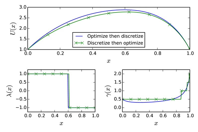
(a) $M=128$

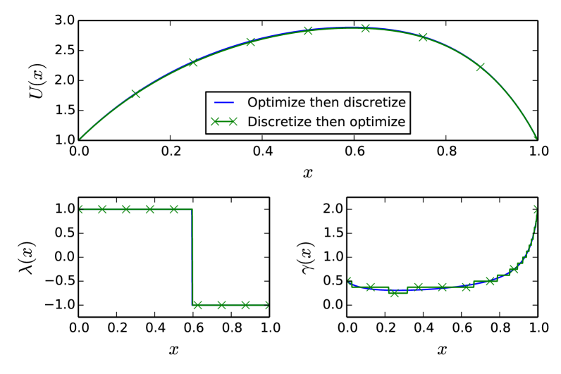
(b) $M=512$

Figure 2: Solution and controls computed by both schemes (parameters used: (21))

In this subsection, we apply the OD and DO schemes (described in the previous subsection and Appendix A, respectively) to compute a numerical solution of (12) under the parameterization

$$\sigma(x,\lambda) =0.2 \alpha(x) =2-x \eta(x) =0.04$$

$$\mu(x,\lambda) =0.04\lambda \beta(x) =1+x g(x) =1$$ (21)

where $\lambda\in\Lambda=\{-1,1\}$. Since $\Lambda$ is finite, we take $\Lambda_{\Delta x}=\Lambda$. For the DO scheme, we take $\gamma_{\max}=2$ and discretize $\Gamma_{0}=[0,\gamma_{\max}]$ by a uniform partition $0=\gamma_{0}<\cdots<\gamma_{K}=\gamma_{\max}$ (see Appendix A for details).

In our implementation of Policy-Iteration, instead of using the terminating condition on line 5 of the algorithm, we terminate the algorithm when it meets the relative error tolerance

$$\left\|u_{(k)}-u_{(k-1)}\right\|_{\infty}\leqslant 10^{-12}+10^{-6}\left\|u_{(k)}\right\|_{\infty}.$$ (22)

In the case of the DO scheme, $m=2$ and $A(P)$ is a tridiagonal matrix (see (25a) and (25b) of Appendix A). Therefore, we use a tridiagonal solver to solve $A(P)x=b(P)$. As for the OD scheme, $m=3$ and we use the Newton’s method described in [10, Section 4] to solve $A(P)x^{2}=b(P)$. Denoting by $x_{(k)}$ the iterates produced by Newton’s method, we terminate the algorithm when it meets the error tolerance

$$\left\|x_{(k)}-x_{(k-1)}\right\|_{\infty}\leqslant 10^{-24}+10^{-12}\left\|x_{(k)}\right\|_{\infty}.$$

Convergence results are given in Table 1, in which we report a representative value of the numerical solution (Value), the relative error (Rel. err.), ratio of errors (Ratio), number of policy iterations (Its.), average number of iterations (Inner its.) to solve the system $A(P)x^{m-1}=b(P)$ if applicable, and total time elapsed in seconds (Time). The representative value of the numerical solution is $u_{\Delta x}(x_{0})$ where $x_{0}=\nicefrac{{1}}{{2}}$ is the midpoint of $\overline{\Omega}$. The relative error is given by

$$\left|\frac{u_{\Delta x}(x_{0})-U(x_{0})}{U(x_{0})}\right|$$

where $U$ is the exact solution. Since the exact solution is generally unavailable, we replace $U$ by the solution computed by the OD scheme at a level of refinement higher than that which is shown in the table. The ratio of errors is given by

$$\frac{u_{\Delta x/2}(x_{0})-u_{\Delta x}(x_{0})}{u_{\Delta x/4}(x_{0})-u_{\Delta x/2}(x_{0})}$$

so that the base-2 logarithm of this quantity gives us an estimate on the order of convergence (e.g., $\text{Ratio}\approx 2$ suggests linear convergence, $\text{Ratio}\approx 4$ suggests quadratic, etc.). Plots of the solution and optimal controls are given in Figure 2.

The OD scheme is faster and more accurate than the DO scheme. Since both schemes require roughly the same number of policy iterations, it follows that the DO scheme loses most of its time on the pivot step on line 3 of Policy-Iteration. As $K\rightarrow\infty$, this effect becomes more pronounced. Note also that the OD scheme exhibits a fairly stable linear order of convergence while that of the DO scheme is erratic.

6.3 A problem which is neither s.d.d. nor weakly irreducibly diagonally dominant

$M$		Value	Rel. err.	Ratio	Its.	Inner. its.	Time
32		3.0703	1.6e$-$1		3	6.67	4.3e$-$2
64		3.3567	8.5e$-$2		3	6.67	3.7e$-$2
128		3.5114	4.3e$-$2	1.85	3	6.67	5.4e$-$2
256		3.5917	2.1e$-$2	1.92	3	6.67	9.3e$-$2
512		3.6327	9.9e$-$3	1.96	3	6.67	1.7e$-$1
1024		3.6534	4.3e$-$3	1.98	3	6.67	3.3e$-$1
2048		3.6638	1.4e$-$3	1.99	3	7.67	6.5e$-$1

(a) Optimize then discretize

$M$	$K$	Value	Rel. err.	Ratio	Its.		Time
32	1	0.9273	7.5e$-$1		3		1.7e$-$2
64	2	1.8839	4.9e$-$1		5		3.9e$-$2
128	4	3.2430	1.2e$-$1	0.70	7		1.4e$-$1
256	8	3.5376	3.6e$-$2	4.61	9		6.4e$-$1
512	16	3.6163	1.4e$-$2	3.74	14		3.5e$+$0
1024	32	3.6490	5.5e$-$3	2.41	15		1.4e$+$1
2048	64	3.6629	1.7e$-$3	2.35	7		2.3e$+$1

(b) Discretize then optimize

Table 2: Convergence results (parameters used: (23))

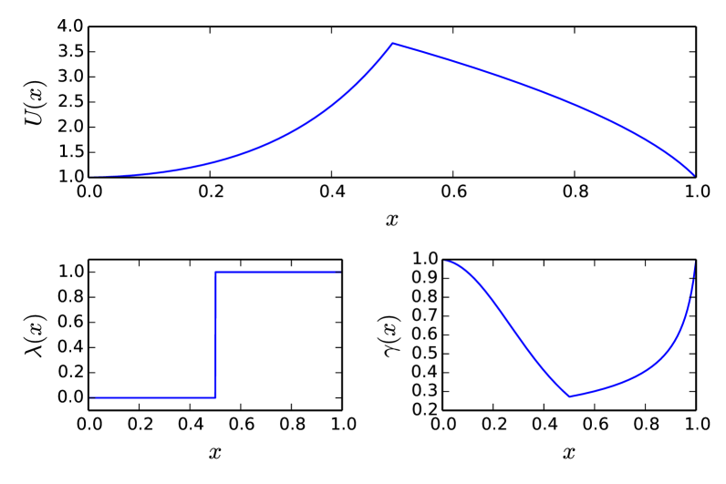
Figure 3: Solution and controls computed (parameters used: (23); OD scheme only)

Figure 4: Directed graph of $A$ defined by (16a) and (16b) with $\sigma$ and $\mu$ given by (23)

We now turn to a parameterization of (12) whose corresponding “discretization tensor” $A(\boldsymbol{\lambda})$ defined by (16a) and (16b) is neither s.d.d. nor weakly irreducibly diagonally dominant. We are motivated by an analogous phenomenon that occurs for classical discretizations of degenerate elliptic differential equations first studied in [6] in which the matrix arising from the discretization is neither s.d.d. nor irreducibly diagonally dominant (cf. [18, 2, 7]).

The parameterization we study is

$$\sigma(x,\lambda) =0.3(1-\lambda) \alpha(x) =1 \eta(x) =\boldsymbol{1}_{\{x\leqslant 0.5\}}(x)$$

$$\mu(x,\lambda) =0.04\lambda \beta(x) =1 g(x) =1$$ (23)

where $\lambda\in\Lambda=\{0,1\}$. Note that this parameterization does not satisfy (A2) or (A3) since $\eta$ is allowed to be zero. Therefore, the argument used to establish that $A(\boldsymbol{\lambda})$ is a strong M-tensor in Section 6.1 fails (see, in particular, (19)).

Letting $\omega$ be any function which maps $\mathbb{R}_{++}$ to itself such that $\lim_{t\rightarrow 0}\omega(t)=0$, one way to get around the above issue is to replace $A(\boldsymbol{\lambda})$ by $A(\boldsymbol{\lambda})+I\omega({\Delta x})$ in (18), since the latter is trivially s.d.d. The obvious downside of this approach is that it introduces additional discretization error.

Fortunately, it turns out that we can directly establish that $A(\boldsymbol{\lambda})$ is a strong M-tensor by relying on the theory of w.c.d.d. tensors. In particular, by (19),

1. $A(\boldsymbol{\lambda})$ is a w.d.d. (not s.d.d.) Z-tensor since $\eta_{i}\geqslant 0$ and

2. $0,M\in J(A(\boldsymbol{\lambda}))$ are s.d.d. rows.

The directed graph of $A(\boldsymbol{\lambda})$ is shown in Figure 4 where we have

1. ignored self-loops of the form $i\rightarrow i$ and

2. used a dashed line to indicate an edge that is present only when $\lambda_{i}=0$.

Note that for any $i\notin J(A(\boldsymbol{\lambda}))$, we can form the walk $i\rightarrow i+1\rightarrow\cdots\rightarrow M$ ending at the s.d.d. vertex $M\in J(A(\boldsymbol{\lambda}))$. Therefore, $A(\boldsymbol{\lambda})$ is w.c.d.d. and hence a strong M-tensor by Theorem 1. Now, by Theorem 29, we can compute a solution of the OD scheme as applied to the parameterization (23) by policy iteration. Convergence results and plots are shown in Table 2 and Figure 3, respectively. The $C^{1}$ discontinuity in the solution is due to the discontinuity in $\eta$.

7 Summary

In this work, we introduced the high order Bellman equation (1), extending classical Bellman equations to the tensor setting. We also introduced w.c.d.d. tensors (Definition 15), also extending the notion of w.c.d.d. matrices to the tensor setting. We established a relationship between w.c.d.d. tensors and M-tensors (Theorem 1), analogous to the relationship between w.c.d.d. matrices and M-matrices [1]. We proved that a sufficient condition to ensure the existence and uniqueness of a positive solution to a high order Bellman equation is that the tensors appearing in the equation are s.d.d. M-tensors (Lemma 23 and Lemma 24). We also showed that the s.d.d. requirement can be relaxed to the weaker requirement of w.c.d.d. so long as we restrict ourselves to a finite set of policies (Lemma 26). In this case, the solution of (1) can be computed by a policy iteration algorithm (Theorem 29). The question of whether or not the assumption of finitude can be removed remains open (Remark 27). We applied our findings to create a so-called “optimize then discretize” scheme for an optimal stochastic control problem which outperforms (in both computation time and accuracy) a classical “discretize then optimize” approach (Section 6). ifclassloadedsiamart1116

Appendix A Discretize then optimize scheme

In this appendix, we derive the DO scheme for the differential equation (12). Since the set $\Gamma=[0,\infty)$ is unbounded, we restrict our attention to controls $\gamma$ in some bounded interval $\Gamma_{0}=[0,\gamma_{\max}]$. To ensure the consistency of the resulting scheme, $\gamma_{\max}$ should be chosen sufficiently large. For each $\Delta x>0$, we let $\Gamma_{\Delta x}$ denote a finite subset of $\Gamma_{0}$ such that $d_{H}(\Gamma_{\Delta x},\Gamma_{0})\rightarrow 0$ as $\Delta x\downarrow 0$. The DO discretization is given by the $M+1$ equations

$$\begin{cases}-{\displaystyle\max_{(\gamma,\lambda)\in\Gamma_{\Delta x}\times\Lambda_{\Delta x}}}\left\{(L_{\Delta x}^{\lambda}u)_{i}-\eta_{i}u_{i}-\frac{1}{2}\alpha_{i}\gamma^{2}u_{i}+\beta_{i}\gamma\right\}=0,&\text{for }0<i<M\\ u_{i}=g_{i}&\text{for }i=0,M\end{cases}$$ (24)

where the various quantities $L_{\Delta x}^{\lambda}$, $\eta_{i}$, etc. are defined in Section 6.1 (compare (24) with the OD discretization (14)).

We can transform (24) into a classical $m=2$ Bellman equation as follows. Define the Cartesian product $\boldsymbol{\Gamma}_{\Delta x}=(\Gamma_{\Delta x})^{M+1}$ and denote by $\boldsymbol{\gamma}=(\gamma_{0},\ldots,\gamma_{M})$ an element of $\boldsymbol{\Gamma}_{\Delta x}$ with $\gamma_{i}\in\Gamma_{\Delta x}$. Define $\boldsymbol{\Lambda}_{\Delta x}$ and $\boldsymbol{\lambda}=(\lambda_{0},\ldots,\lambda_{M})$ similarly. Let $A(\boldsymbol{\gamma},\boldsymbol{\lambda})=(a_{ij}(\boldsymbol{\gamma},\boldsymbol{\lambda}))$ be the tridiagonal matrix whose only nonzero entries are

$$a_{i,i-1}(\boldsymbol{\gamma},\boldsymbol{\lambda}) =-\frac{1}{2}\sigma_{i}(\lambda_{i})^{2}\frac{1}{(\Delta x)^{2}}+\phantom{|}\mu_{i}(\lambda_{i})\phantom{|}\frac{1}{\Delta x}\boldsymbol{1}_{(-\infty,0)}(\mu_{i}(\lambda_{i})),$$

$$a_{i,i}(\boldsymbol{\gamma},\boldsymbol{\lambda}) =+\frac{1}{2}\sigma_{i}(\lambda_{i})^{2}\frac{2}{(\Delta x)^{2}}+|\mu_{i}(\lambda_{i})|\frac{1}{\Delta x}+\eta_{i}+\frac{1}{2}\alpha_{i}\gamma_{i}^{2}, \text{if }0<i<M$$ (25a)

$$a_{i,i+1}(\boldsymbol{\gamma},\boldsymbol{\lambda}) =-\frac{1}{2}\sigma_{i}(\lambda_{i})^{2}\frac{1}{(\Delta x)^{2}}-\phantom{|}\mu_{i}(\lambda_{i})\phantom{|}\frac{1}{\Delta x}\boldsymbol{1}_{(0,+\infty)}(\mu_{i}(\lambda_{i})),$$

and

$$a_{i,i}(\boldsymbol{\gamma},\boldsymbol{\lambda})=1,\qquad\text{if }i=0,M.$$ (25b)

Lastly, define the vector $b(\boldsymbol{\gamma})=(b_{0}(\boldsymbol{\gamma}),\ldots,b_{M}(\boldsymbol{\gamma}))$ by

$$b_{i}(\boldsymbol{\gamma})=\begin{cases}{\displaystyle\beta}_{i}\gamma_{i},&\text{if }0<i<M\\ g_{i},&\text{if }i=0,M.\end{cases}$$

Then, the discrete equations (24) are equivalent to the classical Bellman equation

$$\min_{(\boldsymbol{\gamma},\boldsymbol{\lambda})\in\boldsymbol{\Gamma}_{\Delta x}\times\boldsymbol{\Lambda}_{\Delta x}}\left\{A(\boldsymbol{\gamma},\boldsymbol{\lambda})u-b(\boldsymbol{\gamma})\right\}=0.$$

The downside of the above approach is twofold:

1. The size of the policy set is $|\mathcal{P}|=|\boldsymbol{\Gamma}_{\Delta x}||\boldsymbol{\Lambda}_{\Delta x}|$. In the OD approach, the size of the policy set is $|\mathcal{P}|=|\boldsymbol{\Lambda}_{\Delta x}|$ (recall that the policy iteration algorithm takes, in the worst case, $|\mathcal{P}|$ iterations).

2. Assuming $\gamma_{\max}$ is chosen large enough, the approximation of $\Gamma_{0}$ by $\Gamma_{\Delta x}$ introduces $O(d_{H}(\Gamma_{\Delta x},\Gamma_{0}))$ local truncation error.

References

- [1] P. Azimzadeh, A fast and stable test to check if a weakly diagonally dominant matrix is a nonsingular M-matrix, Math. Comp., (2018).
- [2] P. Azimzadeh and P. A. Forsyth, Weakly chained matrices, policy iteration, and impulse control, SIAM J. Numer. Anal., 54 (2016), pp. 1341–1364, https://doi.org/10.1137/15M1043431.
- [3] G. Barles and P. E. Souganidis, Convergence of approximation schemes for fully nonlinear second order equations, Asymptotic Anal., 4 (1991), pp. 271–283.
- [4] J. T. Betts and S. L. Campbell, Discretize then optimize, in Mathematics for industry: challenges and frontiers, SIAM, Philadelphia, PA, 2005, pp. 140–157.
- [5] O. Bokanowski, S. Maroso, and H. Zidani, Some convergence results for Howard’s algorithm, SIAM J. Numer. Anal., 47 (2009), pp. 3001–3026, https://doi.org/10.1137/08073041X.
- [6] J. H. Bramble and B. E. Hubbard, On a finite difference analogue of an elliptic boundary problem which is neither diagonally dominant nor of non-negative type, J. Math. and Phys., 43 (1964), pp. 117–132.
- [7] Y. Chen, J. W. L. Wan, and J. Lin, Monotone mixed finite difference scheme for Monge-ampère equation, Journal of Scientific Computing, (2018).
- [8] M. G. Crandall, H. Ishii, and P.-L. Lions, User’s guide to viscosity solutions of second order partial differential equations, Bull. Amer. Math. Soc. (N.S.), 27 (1992), pp. 1–67, https://doi.org/10.1090/S0273-0979-1992-00266-5.
- [9] W. Ding, L. Qi, and Y. Wei, M-tensors and nonsingular M-tensors, Linear Algebra Appl., 439 (2013), pp. 3264–3278, https://doi.org/10.1016/j.laa.2013.08.038.
- [10] W. Ding and Y. Wei, Solving multi-linear systems with M-tensors, J. Sci. Comput., 68 (2016), pp. 689–715, https://doi.org/10.1007/s10915-015-0156-7.
- [11] P. A. Forsyth and G. Labahn, Numerical methods for controlled Hamilton-Jacobi-Bellman PDEs in finance, Journal of Computational Finance, 11 (2007).
- [12] S. Friedland, S. Gaubert, and L. Han, Perron-Frobenius theorem for nonnegative multilinear forms and extensions, Linear Algebra Appl., 438 (2013), pp. 738–749, https://doi.org/10.1016/j.laa.2011.02.042.
- [13] S. Hu, Z. Huang, and L. Qi, Strictly nonnegative tensors and nonnegative tensor partition, Sci. China Math., 57 (2014), pp. 181–195, https://doi.org/10.1007/s11425-013-4752-4, https://doi.org/10.1007/s11425-013-4752-4.
- [14] H. J. Kushner and P. G. Dupuis, Numerical methods for stochastic control problems in continuous time, vol. 24 of Applications of Mathematics (New York), Springer-Verlag, New York, 1992, https://doi.org/10.1007/978-1-4684-0441-8.
- [15] A. M. Oberman, Convergent difference schemes for degenerate elliptic and parabolic equations: Hamilton-Jacobi equations and free boundary problems, SIAM J. Numer. Anal., 44 (2006), pp. 879–895, https://doi.org/10.1137/S0036142903435235.
- [16] L. Qi, Eigenvalues of a real supersymmetric tensor, J. Symbolic Comput., 40 (2005), pp. 1302–1324, https://doi.org/10.1016/j.jsc.2005.05.007.
- [17] L. Qi and Z. Luo, Tensor analysis, Society for Industrial and Applied Mathematics, Philadelphia, PA, 2017, https://doi.org/10.1137/1.9781611974751.ch1. Spectral theory and special tensors.
- [18] P. N. Shivakumar, J. J. Williams, Q. Ye, and C. A. Marinov, On two-sided bounds related to weakly diagonally dominant -matrices with application to digital circuit dynamics, SIAM J. Matrix Anal. Appl., 17 (1996), pp. 298–312, https://doi.org/10.1137/S0895479894276370.
- [19] N. Touzi, Optimal stochastic control, stochastic target problems, and backward SDE, vol. 29 of Fields Institute Monographs, Springer, New York; Fields Institute for Research in Mathematical Sciences, Toronto, ON, 2013, https://doi.org/10.1007/978-1-4614-4286-8. With Chapter 13 by Angès Tourin.
- [20] L. Zhang, L. Qi, and G. Zhou, M-tensors and some applications, SIAM J. Matrix Anal. Appl., 35 (2014), pp. 437–452, https://doi.org/10.1137/130915339.