How does monetary policy affect income inequality in Japan? Evidence from grouped data

Abstract

We examine the effects of monetary policy on income inequality in Japan. For that purpose, we use a novel Bayesian approach that jointly estimates the Gini coefficient from grouped income data and the dynamics of macroeconomic quantities. Our results indicate different effects on income inequality for different types of households: A monetary tightening decreases inequality when we consider a broad definition of household data that also includes the unemployed and retirees. Higher unemployment and tighter borrowing conditions make the richer (i.e., employed) comparably worse off. The result reverses, if we focus on the sub-sample of households whose head is employed. Through the same channels, inequality increases if monetary policy is tightened. A counterfactual analysis reveals that indeed the financial channel and the job destruction channel are the most important transmission mechanisms.

Keywords:

Income inequality; Monetary policy; Grouped data; Bayesian analysis.

JEL Codes:

C30, E52, F41, E32.

1 Introduction

While there is a long-standing literature on the nexus between income inequality and economic growth, income distribution and monetary policy have been traditionally considered separate issues. The outbreak of the global financial crisis and the subsequent recession led major central banks to loosen their monetary policy stance. This spiked new interest in the relationship between monetary policy and income inequality – also since a lot of these measures comprised asset purchases by the central bank and it is known that price movements in assets should impact inequality. Hitherto, empirical work did not provide clear evidence, also since transmission channels seem complex and depend on the distribution of financial assets and liabilities in the population - at best, a modest effect of monetary policy on inequality can be found in the data (Amaral, 2017). In recent contributions, Coibion et al. (2017) for the USA, Mumtaz and Theophilopoulou (2017) for the UK and Furceri et al. (2017) for a broader set of countries, a systematic impact of monetary policy on inequality has been established: If monetary policy is tightened, inequality increases.

One reason why the literature on the monetary policy and inequality nexus is scarce might be that effects of monetary policy in a macroeconomic context are frequently addressed within a time series framework such as a vector autoregression (VAR). Income data, however, is often collected in surveys that are available only over a short time period, or isolated years. For example, the Japanese National Survey of Family Income and Expenditure offers very detailed information on household income and expenditures but is carried out every five years only. To circumvent the paucity of continuous time series on income data, researchers have used grouped data that are constructed by aggregating individual observations of a variable into income groups and are available over a longer time horizon. Using these data directly, however, would imply the stark assumption that all households within a group have the same income (Chotikapanich et al., 2007b). A better alternative is to estimate the underlying distribution using suitable econometric tools (see, e.g., Chotikapanich et al., 2007a).

In this paper, we investigate the effects of monetary policy on income inequality in Japan. The Bank of Japan (BoJ) can be considered a front runner in deploying different forms of monetary policy besides interest rate changes (e.g., see Shirakawa, 2010; Bernanke, 2017). From the perspective of other central banks, Japanese data can thus provide useful insights on how these measures affect income inequality. We propose a novel econometric approach that jointly models the Gini coefficient based on grouped income data of households and the dynamics of macroeconomic quantities. In that sense we combine the predominant framework used in monetary economics, VAR models, and the methods used to estimated income distributions. The proposed model is an extension of the work of Nishino et al. (2012) to the VAR case. More precisely, Nishino et al. (2012) estimate income inequality using a state-space representation with the state variable reflecting income inequality. In this paper, we take this approach one step further and include the state variable as an endogenous variable into a VAR system. In other words, our model allows for a coherent and joint estimation of macroeconomic key variables and income inequality. This is a significant improvement over existing approaches that calculate measures of inequality in a first step and treat them as observed data in the subsequent estimations. As pointed out in Carriero et al. (2018) this might lead to a severe bias and flawed inference.

Our main results are as follows. First, we find that the effect of monetary policy on income inequality depends on the household under consideration. A monetary tightening leads to a decrease in inequality if we consider a broader measure of income that also covers households that are unemployed or retired. The Gini decreases since the monetary tightening leads to more unemployment and worse borrowing conditions. Both affect rather the employed households which – compared to the unemployed / retired – makes income more equal. The same channels are at play if we consider the sub-sample of households whose head is employed. However, here, more unemployment and tighter financing conditions lead to more inequality since it affects poorer households – in that sample – more strongly. A counterfactual analysis corroborates that monetary policy transmits most strongly through the unemployment rate and long-term interest rates, while other potential transmission channels such as through inflation or the exchange rate are less important. Our results are robust to different ways of identifying the monetary policy shock and more generally measures of monetary policy.

The paper is structured as follows: The next section introduces the model, while section 3 summarizes the data. Section 4 presents the main findings from the estimation, while section 5 concludes.

2 The model

In this section we describe the econometric approach. We start with outlining the basic idea of how to estimate an income distribution from grouped data. We follow Nishino and Kakamu (2011) and assume that income $x$ is log-normally distributed, $x\sim\mathcal{LN}(\mu,\sigma^{2})$. The associated probability density function (PDF) is then given by

$$f(x|\mu,\sigma^{2})=\frac{1}{x\sqrt{2\pi\sigma^{2}}}\exp\left\{-\frac{(\ln x-\mu)^{2}}{2\sigma^{2}}\right\}.$$

The cumulative density function (CDF) is

$$F(x)=\Phi\left(\frac{\ln x-\mu}{\sigma}\right),$$

where $\Phi(\cdot)$ denotes the CDF of the standard normal distribution. Then, the Gini coefficient based on the lognormal distribution is defined as

$$G=2\Phi\left(\frac{\sigma}{\sqrt{2}}\right)-1,$$

and we notice that the Gini coefficient is a monotone function of $\sigma$.

Assume that the income distribution is $x\sim\mathcal{LN}(\mu,\sigma^{2})$ with $p_{i}$th quantiles ($i=1,\ldots,k$), where $\displaystyle p_{i}=\frac{n_{i}}{n}$ denote the relative frequencies and $1\leq n_{1}<n_{2}<\ldots<n_{k}\leq n$, are observed as $(x_{1},x_{2},\ldots,x_{k})$ from $n$ observations. In the empirical application, $x_{k}$ is going to denote the endpoint of each income category (as opposed to the mean value). Let $\mathbf{x}=(x_{1},x_{2},\ldots,x_{k})^{\prime}$, then by the asymptotic theorem of the selected order statistics,

$$\sqrt{n}(\ln\mathbf{x}-\mu-\sigma\mathbf{u})\sim\mathcal{N}\left(\mathbf{0}_{k},\sigma^{2}\mathbf{W}\right)\quad\text{as $n\to\infty$},$$

where $\mathbf{u}=(u_{1},u_{2},\ldots,u_{k})^{\prime}$, $u_{i}=\Phi^{-1}(p_{i})$, $\Phi^{-1}(\cdot)$ is the inverse distribution function, $\mathbf{0}_{k}=(\underbrace{0,0,\ldots,0}_{k})^{\prime}$ and the $ij$th element of $\mathbf{W}$ is defined as

$$w_{ij}=w_{ji}=\frac{p_{i}(1-p_{j})}{\phi\left(\Phi^{-1}(p_{i})\right)\phi\left(\Phi^{-1}(p_{j})\right)},\quad(i\leq j),$$

where $\phi(\cdot)$ is the PDF of the standard normal distribution. The proof of these asymptotic properties is provided in Nishino and Kakamu (2011). The assumption of a constant variance of the income distribution is relaxed in Nishino et al. (2012). Nishino and Kakamu (2015) show that the income inequality in Japan is indeed persistent and can be modeled using a stochastic volatility model. Here, we follow Nishino and Kakamu (2015) and allow the variances of the income distribution to drift over time.

Let $\mathbf{x}_{t}=(x_{1,t},x_{2,t},\ldots,x_{k,t})^{\prime}$ and $\mathbf{y}_{t}=(y_{1,t},y_{2,t},\ldots,y_{m,t})^{\prime}$ be the income data and macroeconomic variables of the $t$th period ($t=1,2,\ldots,T$), respectively. Then, we propose the following joint model:

$$\ln\mathbf{x}_{t} = \mu_{t}+\exp(h_{t}/2)\mathbf{u}_{t}+\exp(h_{t}/2)\text{\boldmath{$\epsilon$}}_{t},\quad\text{\boldmath{$\epsilon$}}_{t}\sim\mathcal{N}\left(\mathbf{0}_{k},\mathbf{W}_{t}^{*}\right),$$ (2.1)

$$\mathbf{y}_{t} = \text{\boldmath{$\alpha$}}+\mathbf{B}\mathbf{y}_{t-1}+\text{\boldmath{$\eta$}}_{t},\quad\text{\boldmath{$\eta$}}_{t}\sim\mathcal{N}\left(\mathbf{0}_{m},\mathbf{\Sigma}\right),$$ (2.2)

where $\mathbf{u}_{t}=(u_{1,t},u_{2,t},\ldots,u_{k,t})^{\prime}$, $\displaystyle\mathbf{W}_{t}^{*}=n_{t}^{-1}\mathbf{W}_{t}$, $y_{1,t}=h_{t}$, $\alpha$ is an $m\times 1$ vector of parameters, and $\mathbf{B}$ and $\mathbf{\Sigma}$ are $m\times m$ matrices of parameters, and we assume $\mathbf{y}_{0}=\mathbf{0}_{m}$ for simplicity. In the empirical section, we use 1 lag.

The likelihood function of this model is written as

$$L(\mathbf{X}|\mathbf{Y},\text{\boldmath{$\mu$}},\text{\boldmath{$\alpha$}},\mathbf{B},\mathbf{\Sigma})$$

$$\propto \int\cdots\int\prod_{t=1}^{T}\exp\left(-\frac{h_{t}}{2}\right)\exp\left(-\frac{\mathbf{v}_{t}^{\prime}\mathbf{W}_{t}^{*-1}\mathbf{v}_{t}}{2\exp(h_{t})}\right)|\mathbf{\Sigma}|^{-\frac{1}{2}}\exp\left(-\frac{\mathbf{e}_{t}^{\prime}\mathbf{\Sigma}^{-1}\mathbf{e}_{t}}{2}\right)dh_{1}\ldots dh_{T},$$

where $\mathbf{X}=(\mathbf{x}_{1},\mathbf{x}_{2},\ldots,\mathbf{x}_{T})$, $\text{\boldmath{$\mu$}}=(\mu_{1},\mu_{2},\ldots,\mu_{T})^{\prime}$, $\mathbf{v}_{t}=\ln\mathbf{x}_{t}-\mu_{t}-\exp(h_{t}/2)\mathbf{u}_{t}$, $\mathbf{e}_{t}=\mathbf{y}_{t}-\text{\boldmath{$\alpha$}}-\mathbf{B}\mathbf{y}_{t-1}$, $\mathbf{h}=(h_{1},h_{2},\ldots,h_{T})^{\prime}$, and $\mathbf{Y}=(\mathbf{y}_{1},\mathbf{y}_{2},\ldots,\mathbf{y}_{T})=(\mathbf{h},\mathbf{Y}^{*\prime})^{\prime}$.

It is noteworthy to stress that our proposed model reflects a joint estimation strategy of the measure of income inequality and the macroeconomic vector autoregressive model. An alternative often pursued in the literature would be to treat estimated Gini coefficients as observed data thereby neglecting inherent estimation uncertainty. As pointed out in Carriero et al. (2018) these “two-step” procedures potentially lead to flawed inference. More precisely and in the context of income inequality, in case the Gini is calculated by descriptive statistics using grouped data, inequality tends to be underestimated. This point is illustrated in Fig. 1 below:

[INCLUDE Fig. 1 HERE]

Fig. 1: Lorenz curve and its Gini coefficient

Notes: The plot shows the Gini area based on simulated data for two cases: In red, the Gini is calculated using grouped data from the simulation, whereas in red and blue the Gini is derived directly from the simulated data. The blue area shows the difference between the two.

For the true Lorenz curve (solid line) we assume a log-normal distribution; the Lorenz curve based on grouped data (dotted line) is based on repeated draws from a log-normal distribution. The Gini coefficient derived from grouped data is shown by the red area, while the one for the true distribution covers the red and blue area. The graph illustrates that the Gini coefficient from grouped data (red area) cannot capture the full area (blue area). The reason behind is the underlying assumption of equal income within each group and this assumption leads to an underestimation of inequality, especially in the top income group.

In what follows, we are going to use Bayesian methods to estimate the joint model outlined in equations (2.1) and (2.2) and assume the subsequent prior distributions: $\mu_{t}\sim\mathcal{N}(\mu_{0},\tau_{0}^{2})$, $t=1,2,\ldots,T$, $\text{\boldmath{$\beta$}}\sim\mathcal{N}(\text{\boldmath{$\beta$}}_{0},\mathbf{\Omega}_{0})$, $\mathbf{\Sigma}\sim\mathcal{IW}(\nu_{0},\mathbf{\Sigma}_{0})$. In addition, we set hyper-parameters as $\mu_{0}=0$, $\tau_{0}^{2}=100$, $\text{\boldmath{$\beta$}}_{0}=\mathbf{0}$, $\mathbf{\Omega}_{0}=100\cdot\mathbf{I}$, $\nu_{0}=m+1$ and $\mathbf{\Sigma}_{0}=0.01\cdot\mathbf{I}$, which make the variance of prior distributions diffuse. In the empirical analysis, we run the MCMC algorithm, which is described in Appendix A, for $10,000$ iterations after a burn-in phase of $10,000$ iterations.

3 Data

Following Lise et al. (2014) and Inui et al. (2017) we derive the Gini coefficient using the Japanese household survey called Family Income and Expenditures Survey (FIES), which is compiled by the Statistics Bureau of the Ministry of Internal Affairs and Communications. The survey is carried out on a monthly basis and collects data on earnings, income and consumption expenditures for about 9,000 households and is appropriately adjusted to make the sample size to $n_{t}=n=10,000$ in order to compensate the difference in sampling ratios for strata. The survey unit are households in the entire area of Japan. We use the monthly subset of the survey that covers household incomes and expenditures. Each wave of the survey offers among other data on consumption expenditure, the frequency distribution over 18 groups of yearly pre-tax income: $\mathbf{x}_{t}=\mathbf{x}=(200,250,300,350,400,450,500,550,600,650,700,750,800,900,$
$1000,1250,1500)^{\prime}$, which are collected from Table 8-2 “Amounts of Savings and Liabilities Held per Household by Yearly Income Group”. Income data refers to actual income including tax (i.e., the sum of cash income of all household members), cash on hand carried over from previous months, and so-called “spurious income”. The latter is defined as an increase in cash accompanied by a decrease in assets and increase in liabilities. As an example, the sale of a house generates cash, but decreases households assets. By the same token, if a household borrows money from a bank, cash increases in parallel with household’s liabilities. Both cash increases would be labeled spurious income and are included in overall pre-tax income of households. The 10,000 surveyed households can be roughly divided into two groups: workers’ households are those whose heads are employed as clerks or wage earners by public or private enterprises, such as government office, private companies, factories, schools, hospitals, and shops. Workers’ households account for roughly half of the 10,000 observations in each survey wave. All households include on top of workers’ households, those whose heads are individual proprietors (e.g., merchants, artisans, administrators of unincorporated enterprise, farmers, about 10% of all observations) and those with no occupation (unemployed and retired, about 35% of all observations). Due to changes in the sample design and to get a consistent income series our data starts from 2002Q1.

Pre-tax income data are complemented by macroeconomic data such as real GDP (rgdp), the unemployment rate (unempl), 10-year government bond yields (ltir), the real effective exchange rate (reer) and stock market prices (eq) measured by the NIKKEI225 index. As pointed out in Amaral (2017), inflation expectations are a crucial determinant of inequality. We measure inflation expectations, as one-year ahead projections of consumer price inflation (p). Inflation forecasts are obtained from the IMF’s biannual world economic outlook database and converted to quarterly frequency by reusing the biannual observations over the quarterly frequency domain. Last, we include several measures for the monetary policy stance of the BoJ. These include the the shadow rate (ssr) of Wu and Xia (2016), the 2-year government bond yields (2ygby) as well as the recently proposed target and path factors of Kubota and Shintani (2020). Exchange rate data stem from the BIS and an increase denotes an appreciation in real terms; all other macroeconomic data are obtained via the FRED database, https://fred.stlouisfed.org/. Our sample for the combined income and macro data spans the period from 2002Q1 to 2018Q4.

In a first step and to assess the accuracy of the proposed modeling framework, we plot the estimated Gini coefficient over time. The results are depicted in Fig. 2. The figure reveals some interesting differences of the development of income inequality between the two sub-samples we use. Inequality for all households was very high at the beginning of the sample period, more modest during the period from 2004 to 2013 after which the Gini picked up again. The latest observations from 2018 indicate a significantly higher level of inequality than during the middle of our sample period, surpassing even the peak value of 0.3 at the beginning of the sample. The Gini coefficient based on data for workers’ households shows a different picture: While the estimated Gini coefficient was high at the beginning of the sample period (as for all households), inequality has later embarked on a declining trend. More so, the Gini coefficient was significantly smaller in the most recent period compared to the beginning of the sample. Our estimates are well in line with other Gini coefficients derived from descriptive statistics as in Inui et al. (2017) and Saiki and Frost (2014).

Fig. 2: Estimated Gini coefficient

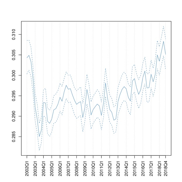
(a) All households

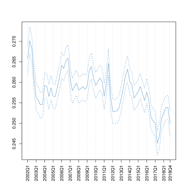
(b) Workers’ households

Notes: The plot shows the estimated Gini coefficient for all households (left panel) and workers’ households (right panel). Posterior median along with 95% credible intervals shown.

4 The effects of monetary policy on inequality

To assess the effects of monetary policy shocks on income inequality we have estimated the vector autoregression in equ. 2.2 that jointly models the dynamics of income inequality (i.e., the Gini coefficient) and the macroeconomic variables.

There are three prominent channels through which monetary policy might affect income inequality. First, the inflation tax channel postulates that a decrease in inflation, after a monetary policy tightening disproportionately affects purchasing power of households at the lower end of the income distribution since these typically hold more cash (Erosa and Ventura, 2002). This would imply less inequality. Second, the earnings heterogeneity or job destruction channel states that income / occupation of poorer households is more strongly shaped by changes in the unemployment rate than that of richer households for which hourly wages are a more prominent factor as a determinant of income (Amaral, 2017). This implies that if unemployment rises due to the monetary policy tightening, poorer households are disproportionately more strongly affected and income inequality increases (Inui et al., 2017). Last, the income composition channel applies if households in different segments of the income distribution rely on different sources of income (e.g., labor, business and capital, see Amaral, 2017, for more details.). Depending on the distribution of income sources, the effect of an interest rate increase might be either inequality reducing or enhancing and thus remains to be empirically assessed. Our data allows us to examine these channels also with respect to different occupations. More specifically, we can examine whether the income distribution of unemployed and retirees (contained in all households data) responds differently from the employed population (workers households). That the occupational status of the household can trigger different effects of how monetary policy affects income inequality has been stressed in e.g., in Gornemann et al. (2012).

Against the backdrop of prolonged periods of near zero interest rates, choosing a suitable policy instrument to model monetary policy in Japan is not straightforward. While in the early studies, monetary policy was thought to mainly work through short-term interest rates (Miyao, 2000, 2002), other measures such as shadow rates (Iwasaki and Sudo, 2017), longer-term yields (Saiki and Frost, 2014; Spiegel and Tai, 2018) or external instruments (Honda and Kuroki, 2006; Kubota and Shintani, 2020) have been considered more recently. Our approach to tackling uncertainty about the policy instrument is to provide a baseline instrument along with several robustness estimations. As a baseline measure, we use the shadow rate of Wu and Xia (2016). This shadow rate is extracted using a term structure model that allows the relaxation of the zero lower bound of nominal short-term rates. During normal times the shadow rate mimics short-term interest rates; in times short-term rates are stuck at the zero lower bound and the central bank provides additional stimulus, the shadow rate can become negative. It thus indicates the monetary policy stance of a central bank even if actual interest rates are zero, which is the case for the sample period we cover. In a robustness exercise we follow Spiegel and Tai (2018) who use 2-year Japanese government bond yields as the policy instrument. We also consider two recently proposed external instruments, namely the target and the path factor of Kubota and Shintani (2020). Both instruments exploit high frequency variation of euro-yen Tokyo interbank offered rates (TIBOR) at different maturities, around policy announcements of the BoJ. The target factor is more reminiscent of conventional / interest rate monetary policy, whereas the path factor tends to affect the longer end of the yield curve reflecting unconventional monetary policies.

As outlined above, all three instruments can be considered as broad monetary policy measures and hence also cover aspects of unconventional monetary policy. This is essential given the macroeconomic environment in Japan over the sample period. That said, one could argue that unconventional monetary policy rather affects wealth than income inequality: bringing down long-term yields mostly impacts financial markets and wealth of households holding these assets. Nevertheless, some effects should be also seen on the distribution of income. Foremost, the spurious income component of our income data is naturally affected by asset / house price movements. Moreover, since (longer-term) interest rates are moved, some of the channels mentioned above could also be operational and income inequality affected. Also, Saiki and Frost (2014) who examine the effects of the BoJ’s asset purchases, report a strong empirical correlation between income and wealth inequality in Japan and Inui et al. (2017) find that distributions of households’ financial assets and liabilities do not play a significant role in the distributional effects of monetary policy. Hence an assessment of monetary policy on income inequality in Japan seems warranted.

To identify the monetary policy shock, we rely on a simple Cholesky decomposition, which requires categorizing the set of macroeconomic variables into slow and fast moving variables. This “recursiveness” assumption has been frequently used in the literature on Japanese monetary policy shocks (Miyao, 2000, 2002) and its implications are discussed more generally in, among others, Christiano et al. (1999). We assume the following ordering of variables:

$$\mathbf{y}_{t}=\left(\begin{array}[]{c}\text{gini}\\ \text{rgdp}\\ \text{p}\\ \text{unempl}\\ \text{shadow rate}\\ \text{ltir}\\ \text{reer}\\ \text{eq}\end{array}\right).$$

The ordering implies that the Gini coefficient, real GDP, inflation expectations and the unemployment rate do not react within the same quarter to an unexpected increase in the policy rate. By contrast, long-term interest rates, the exchange rate and equity prices are allowed to react immediately to a monetary policy shock. The shock is calibrated as a +100bp increase in the policy instrument. Note that in what follows we report estimates of $\sigma$ as the “Gini coefficient” rather than its monotone transform $G$.

Our main results are provided in Figures 3 and 4. The figures show the whole posterior distribution of impulse responses along the median and 68% credible intervals.

[INCLUDE Fig. 3 HERE]

Fig. 3: Responses to an increase in the shadow rate - all households

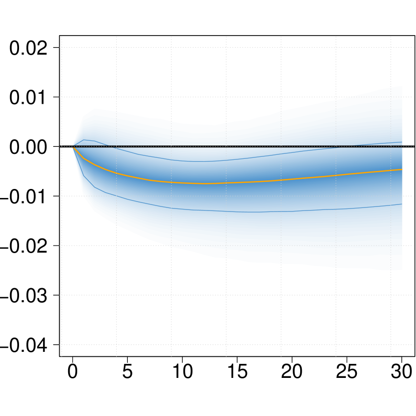
(a) Gini

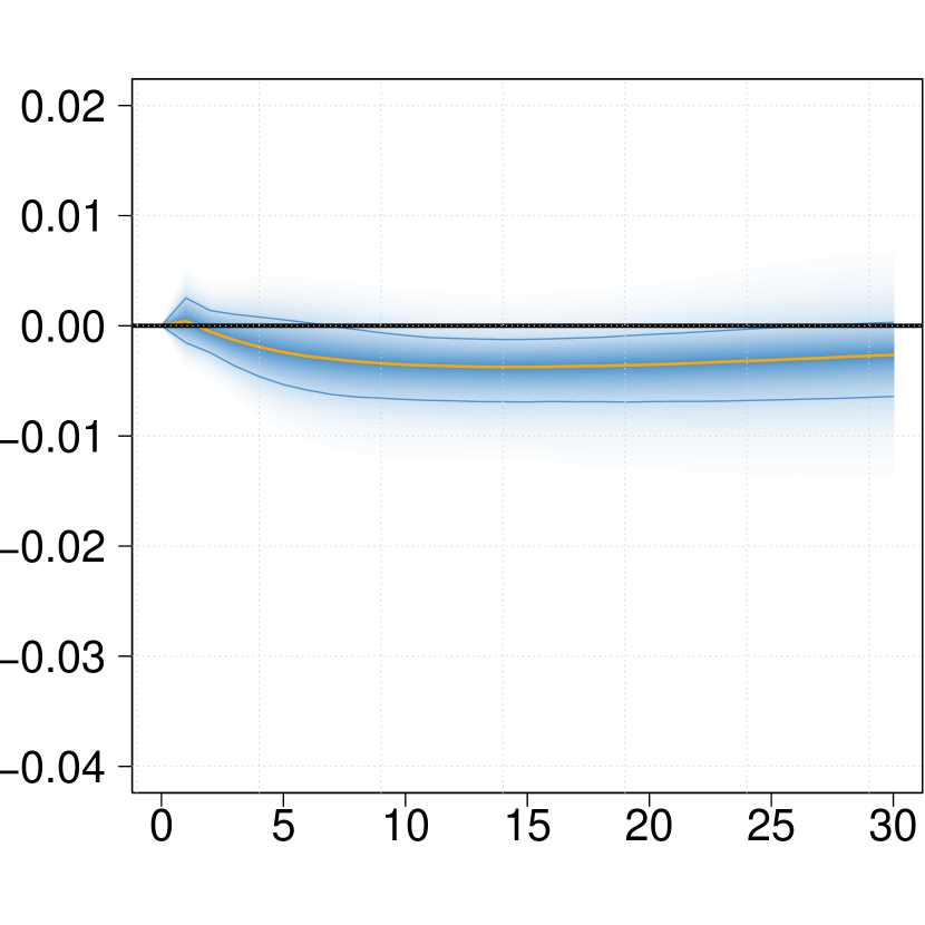
(b) Real GDP

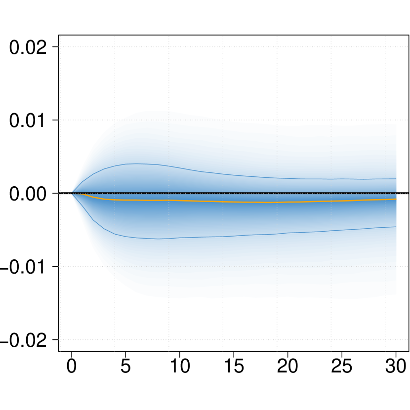
(c) Inflation expectations

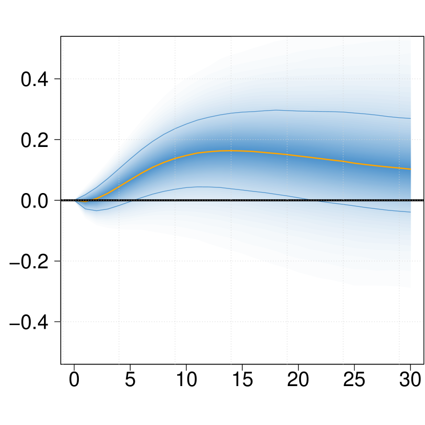
(d) Unemployment rate

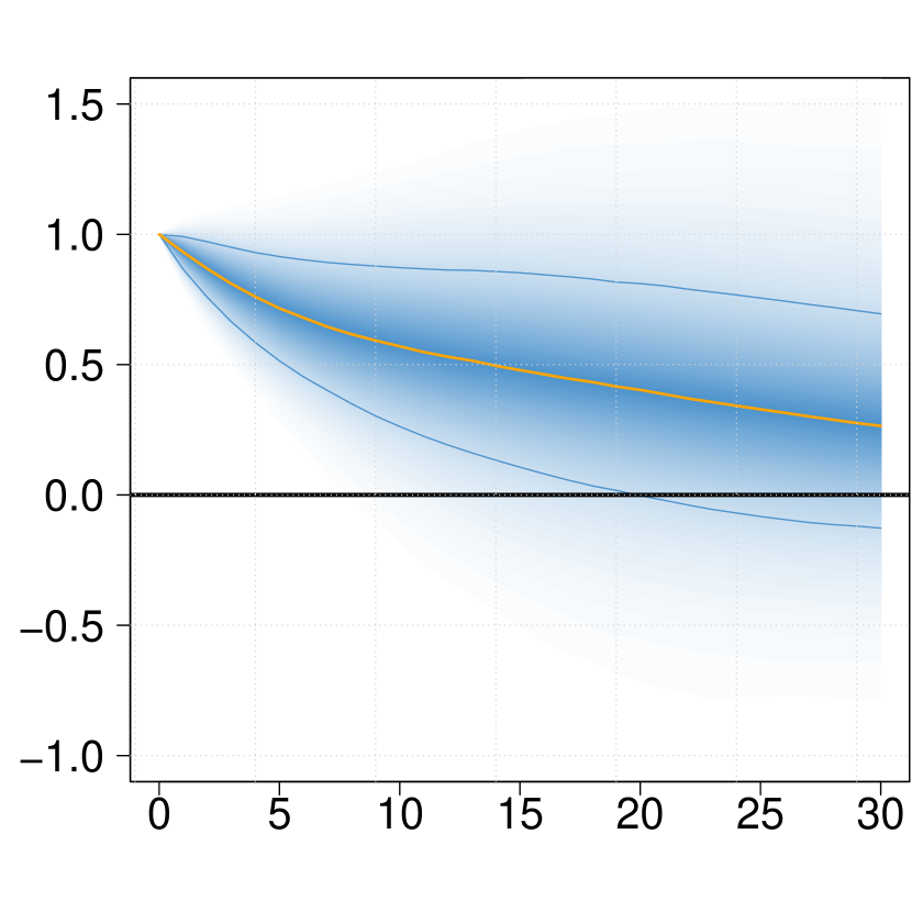
(e) Shadow rate

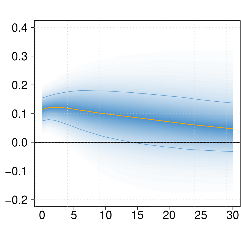
(f) Long rates

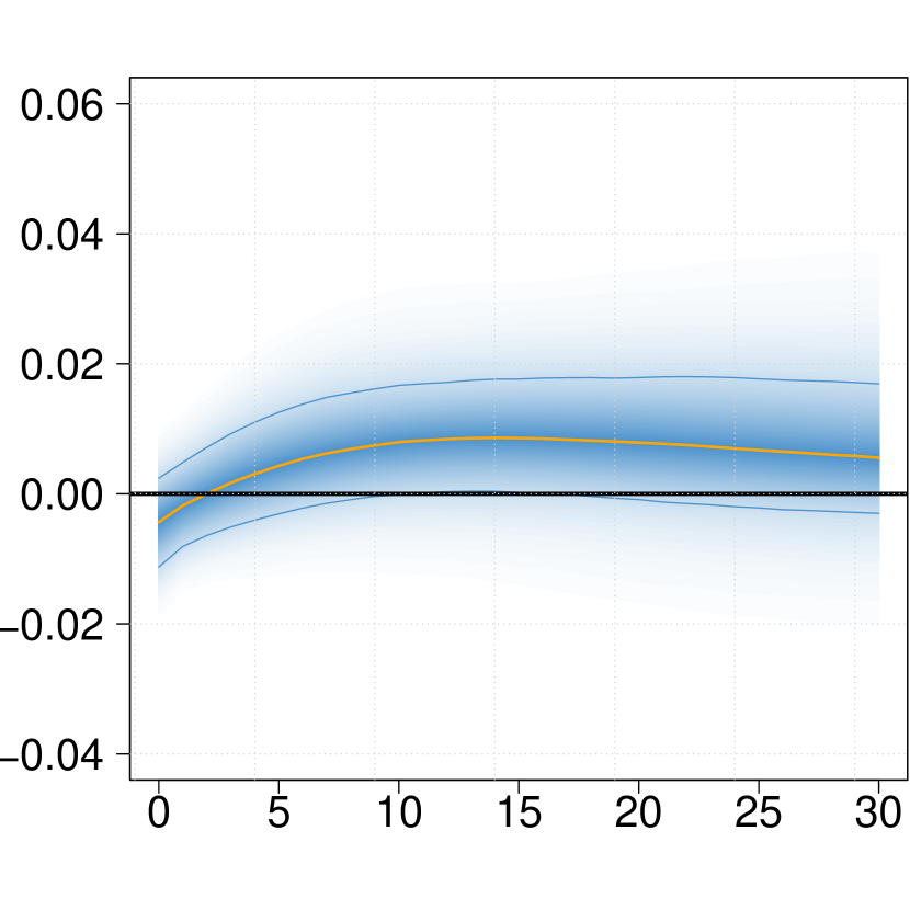
(g) Real eff. exchange rate

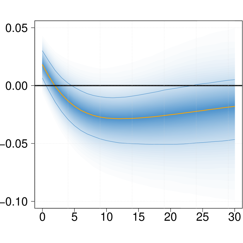
(h) Equity prices

Notes: The plot shows the full posterior distribution of structural responses to a +100bp increase in the shadow rate using a Cholesky decomposition. Posterior median in orange along 68% credible sets (in blue). An increase in the real effective exchange rate corresponds to an appreciation.

[INCLUDE Fig. 4 HERE]

Fig. 4: Responses to an increase in the shadow rate - workers’ households

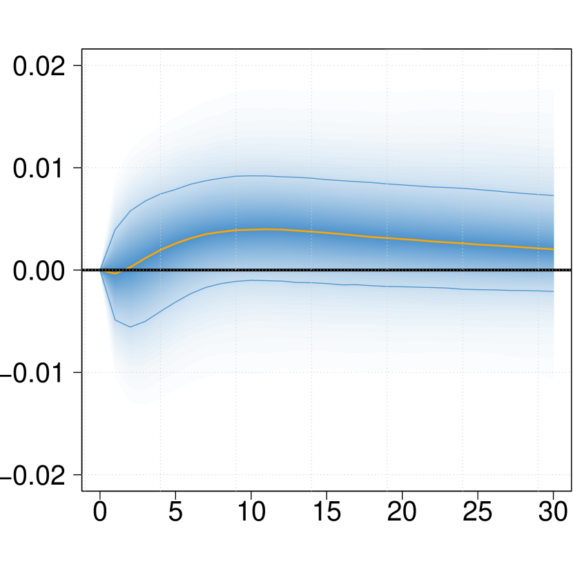
(a) Gini

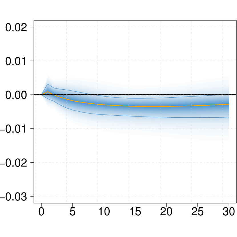
(b) Real GDP

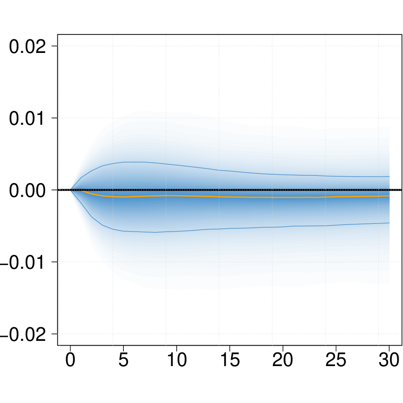
(c) Inflation expectations

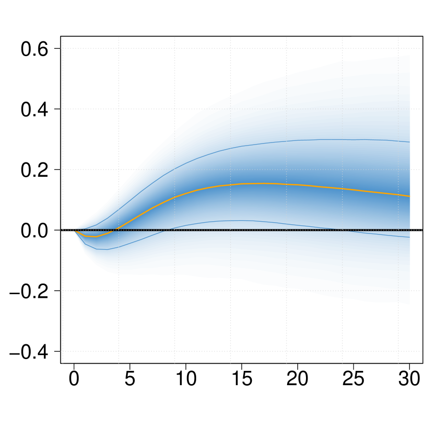
(d) Unemployment rate

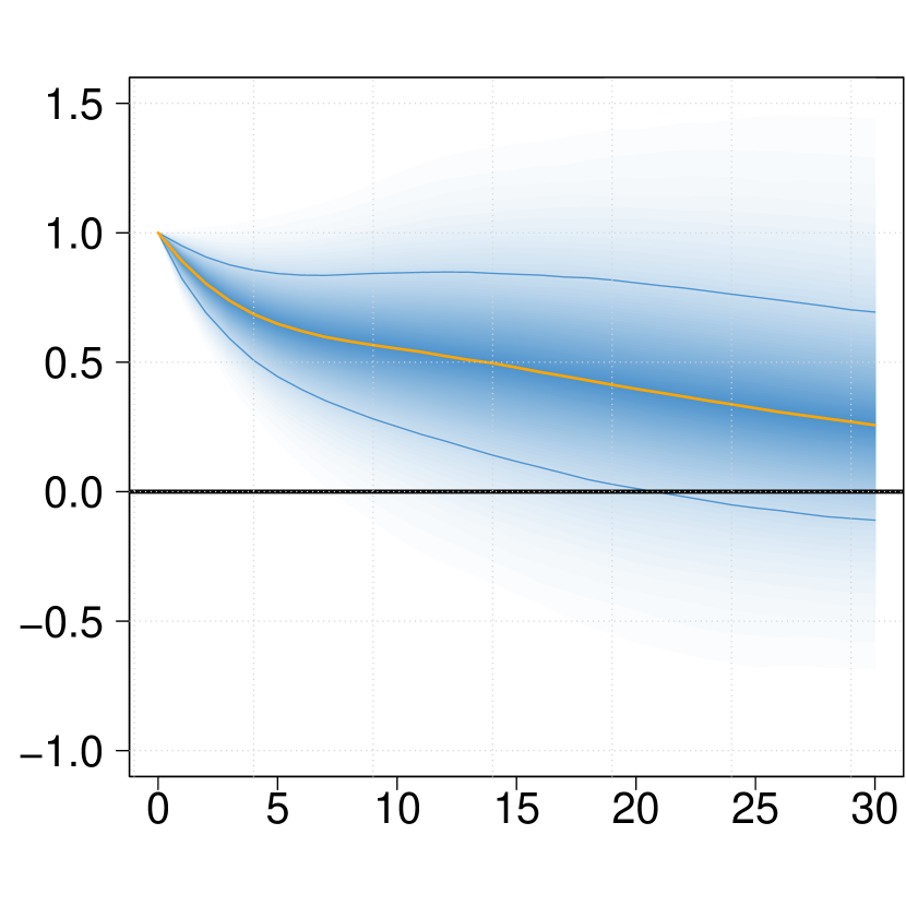
(e) Shadow rate

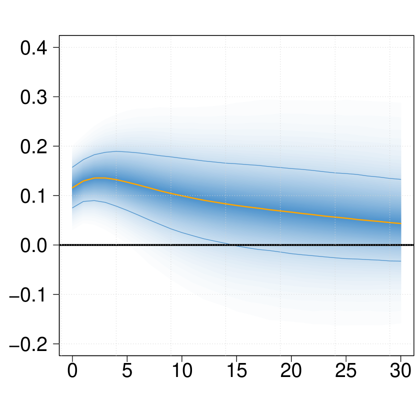
(f) Long rates

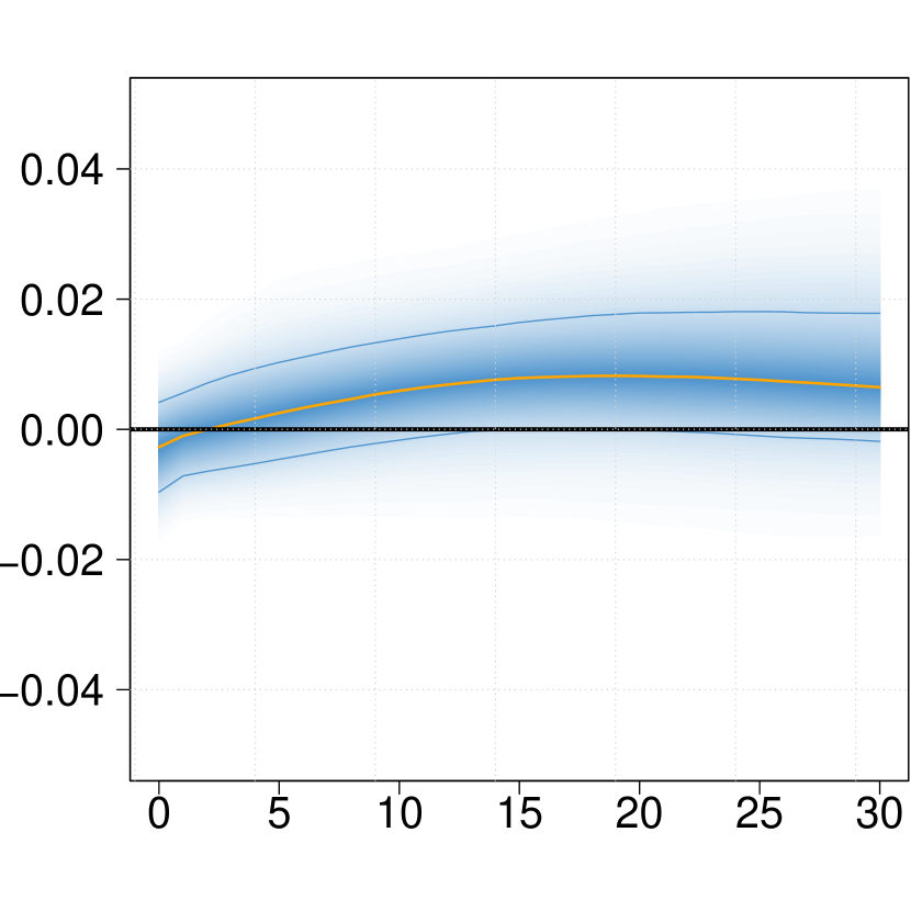
(g) Real eff. exchange rate

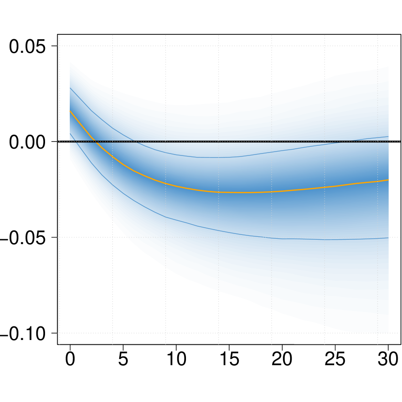
(h) Equity prices

Notes: The plot shows the full posterior distribution of structural responses to a +100bp increase in the shadow rate using a Cholesky decomposition. Posterior median in orange along 68% credible sets (in blue). An increase in the real effective exchange rate corresponds to an appreciation.

We first consider our results for the larger sample that includes all households, depicted in Fig. 3. Here, we find that in response to the monetary tightening, output declines and unemployment rises over the medium-term. We also find a small but not precisely estimated negative effect on inflation expectations. Furthermore the monetary tightening induces an appreciation of the real effective exchange rate and an increase in long-term yields. Stock prices show a very similar picture to real output: while they initially pick up, there is a persistent decline up to about 25 quarters.

Next, we focus on the sub-sample of workers’ households, depicted in Fig. 4. Here, the results are very similar to the ones based on the broader sample: Real GDP declines over the medium term, the unemployment rate rises and inflation expectations fall but not significantly so. We also find evidence for a decrease in stock market prices and a real appreciation of the effective exchange rate.

The fact that the overall responses are very similar for both sub-samples is not surprising since both estimations rely on the same macroeconomic data. Moreover, the direction of responses discussed above are in line with economic theory and qualitatively similar to those provided in Nakajima et al. (2011), who use a more complex time-varying parameter VAR with stochastic volatility. In this sense we do not find evidence for counterintuitive output and price responses often reported for Japanese data.

Turning now to the focal variable, a striking difference between the two samples emerge: The Gini coefficient declines when considering the broader definition of income data (all households, Fig. 3) implying that a monetary policy tightening decreases inequality and rather persistently so. A theoretical explanation for this finding could be through the tax inflation channel, less inflation benefiting the poorer who tend to use more cash. But the response of inflation expectations is small and not precisely estimated. Another and more plausible explanation might be through job destruction, as indicated by a rise in unemployment. Since the sample contains about 35% of unemployed and retirees, more unemployment leads to less inequality. It makes the whole sample poorer. Also, as long-term interest rates increase implying a tightening in financing conditions, spurious income through new loans, declines. This will also disproportionately affect the part of households which have an active income source, leading to less inequality.

The result reverses, if we consider income data based on households whose head is employed (workers’ households, Fig. 4). More specifically, the effect on the Gini is positive, but not precisely estimated. A positive effect on income inequality after a monetary tightening would be in line with estimates of Coibion et al. (2017) for the USA and theoretical predictions based on a New Keynesian model provided in Gornemann et al. (2012). The rise in unemployment, tighter financing conditions through higher long-term rates and a real appreciation, which causes firms in the tradable sector to either lay of workers or cut wages, all could lead to more inequality among the Japanese workforce. We elaborate more on the relative strength of these transmission channels in the next section.

Summing up, we find that a tightening of the monetary policy stance, decreases output and equity prices, while the real effective exchange rate appreciates and unemployment rises. These findings hold true for both groups of households and are in line with common economic reasoning, which ensures overall confidence in our estimation strategy. It turns out that these macroeconomic developments have very distinct effects depending on the employment status of the household’s head. In the larger panel, which also contains the unemployed and retirees, income inequality decreases once monetary policy is tightened. This finding is not present, once considering the smaller group of households who are employed. Here, the Gini has a tendency to increase but effects are not precisely estimated.

4.1 Through which channels does monetary policy affect income inequality?

In this section, we investigate the relative strength of the various transmission channels. For that purpose, we construct a sequence of counterfactual shocks that neutralize effects through a particular variable. The difference between the counterfactual response and the unconditional response (i.e., with all channels open) indicates the relative importance of a particular channel.

Recall that the contemporaneous relationships are captured by the lower triangular, structural $m\times m$ matrix $\boldsymbol{Q}$ and $\mathbf{\Sigma}=\boldsymbol{Q}\boldsymbol{Q}^{\prime}$ being a Cholesky decomposition of $\mathbf{\Sigma}$. We are now interested in the effect of a monetary policy shock on the Gini coefficient shutting down effects through a particular channel / variable $j$. Here, we can distinguish between a direct effect and an indirect effect of the monetary policy shock on the Gini. The direct effect can be obtained by $q_{1,5}$, denoting the element in the $k=1$st row and fifth column of $\boldsymbol{Q}$. It is the fifth column since we have ordered the shadow rate as the fifth variable in the VAR, and the first row since the Gini is ordered first. Similarly, the effect of monetary policy on any other variable $j$ is denoted by $q_{j,5}$. The indirect effect of the monetary policy shock on the Gini through variable $j$ is consequently measured by $q_{1,5}\times q_{j,5}$ and additional higher order effects that can arise through the lag structure in the system (Bachmann and Sims, 2012). Following Bachmann and Sims (2012) and Wong (2015), we proceed by constructing a hypothetical shock sequence for equation $j$ that equalizes the response of $j$ to the monetary policy shock. The resulting impulse responses correspond to a hypothetical scenario under which the constructed shock completely offsets the indirect effects through a particular channel. Manipulating the error terms in that way has the advantage of not having to estimate a new structural model.

The results are depicted in Fig. 5. The figure shows the counterfactual responses on the Gini coefficient with a particular variable / channel shut-down in orange and the unconditional response for comparison in blue.

[INCLUDE Fig. 5 HERE]

Fig. 5: Responses of the Gini coefficient to an increase in the shadow rate – different channels switched off

All households

No real GDP

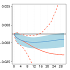
No inflation expectations

No unemployment

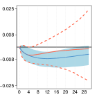
No long rates

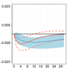
No real eff. exchange rate

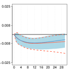
No equity prices

Workers’ households

No real GDP

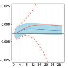
No inflation expectations

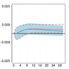
No unemployment

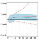
No long rates

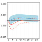
No real eff. exchange rate

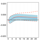
No equity prices

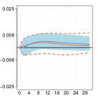
The plot shows the response of the Gini coefficient to a +100bp increase in the shadow rate based on a Cholesky decomposition. In blue, we show the unconditional response, in orange the one with a particular transmission channel switched-off. Posterior median along 68% credible sets. An increase in the real effective exchange rate corresponds to an appreciation.

Examining the relative importance of the channels for the broader household sample shows that the negative response persists for all counterfactual scenarios. In particular we see that counterfactual responses nullifying effects through either inflation or the real effective exchange rate are very similar to the unconditional responses, which leave these channels open. This indicates that these two variable do not play an important role in determining the effects on income inequality. We next consider the unemployment rate. Intuitively and from the perspective of an already unemployed household, other people losing their jobs equalizes the income distribution. Nullifying this effect would result into a slightly less negative effect on the Gini coefficient over the medium term as the orange solid line lies above the blue solid line. This implies that part of the effect of monetary policy on income inequality runs through the unemployment rate. Last and considering financial variables, we do find different adjustment patterns looking at the responses of long-term rates and equity prices. In both cases shutting off responses through financial variables would lead to a sharper but less persistent response of the Gini. That the financial channel is important in transmitting monetary policy is consistent with the fact that monetary policy in Japan during the sample period worked mostly through the longer end of the yield curve and financial markets.

The counterfactual exercise using the sub-sample of workers’ households is contained in the bottom panel of Fig. 5. Here, we see that the Gini tends to increase throughout all counterfactual scenarios. Moreover, counterfactual responses of inflation expectations, the unemployment rate, the exchange rate and equity prices all lead to very similar results compared to the unconditional effect on the Gini. Hence, for the income distribution of workers, these variables seem of less importance in the context of a monetary policy shock. The largest difference between counterfactual and unconditional responses can be observed when looking at effects through long-term interest rates. Here, we see that – in line with unconditional responses of all households – the effect on the Gini would be negative once transmission through long-term rates would be shut-down. This implies that an important channel of monetary policy transmission works through long-term rates: if these increase, overall financing conditions deteriorate and for part of the population it is harder to get a loan (which is included as ”spurious” income in the income data). This leads to more inequality.

Summing up, we find that unemployment and a financial channel both play an important role in determining the effect of monetary policy an inequality for the broad set of households. Both channels render the more equalizing effect of monetary policy more persistent. Most importantly, we find that the difference of distributional effects of monetary policy between workers’ and all households are driven by effects through long-term rates. This implies that tighter financing conditions in the unconditional model are a main driver of inequality.

4.2 Robustness exercises

In this section, we carry out several robustness checks. We start with assessing the role of identification followed by the choice of the policy instrument. Our main results from section 4 are based on a simple Cholesky decomposition using a policy instrument that covers monetary policy in a broad sense. As an alternative to recursive identification, several authors propose using sign restrictions to identify monetary policy shocks (see e.g., Uhlig, 2005). We assume that an unexpected increase in the shadow rate leads to a decrease in output, expected consumer price inflation and equity prices. The assumption on equity prices is based on empirical evidence for the reaction of stock markets to monetary policy-induced interest rate changes (Thorbecke, 1997; Rigobon and Sack, 2004; Bernanke and Kuttner, 2005; Bohl et al., 2017; Li et al., 2010). Last, the unemployment rate is supposed to increase. These restrictions imply that we rule out counterintuitive reactions of prices and output by construction. Naturally, we leave the variable of interest, the Gini, unrestricted. All restrictions are only binding on impact. The results are shown in Fig. 6. We first note that credible intervals tend to be wider compared to the Cholesky-identified responses, which is a typical feature of responses identified through sign restrictions. More precisely, additional uncertainty arises through the need of sampling the rotation matrix necessary to implement sign restrictions. Qualitatively, we find the same effect on the Gini as in our baseline model: The Gini coefficient decreases in response to the monetary policy tightening if we consider the full sample of all households and increases for workers’ households. In both cases, however, estimation uncertainty is considerable as the credible intervals contain zero throughout the response horizon.

Fig. 6: Alternative estimations

Sign restrictions

Gini

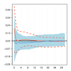
Real GDP

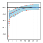
Infl. expect.

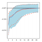
Unempl. rate

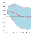
Shadow rates

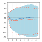
Long rates

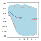
Real eff. exchange rate

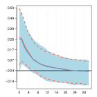
Equity prices

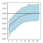
2-year government bond yields

Gini

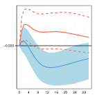
Real GDP

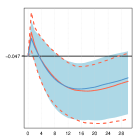
Infl. expect.

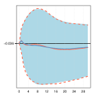
Unempl. rate

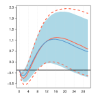
2-year gov. bond yields

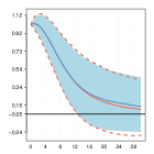
Long rates

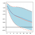
Real eff. exchange rate

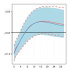
Equity prices

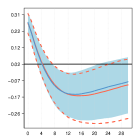
Notes: The plot shows results of a robustness exercise. In the top panel, we show structural responses to a +100bp increase in the shadow rate identified through sign restrictions. In the bottom panel, we show responses to a +100bp increase in 2-year government bond yields using a Cholesky decomposition. For all plots, in blue, results are base on all households, in orange only for workers’ households. Posterior median along 68% credible sets. An increase in the real effective exchange rate corresponds to an appreciation.

Next, we assess how our results are affected when considering identification via external instruments (Gertler and Karadi, 2015; Altavilla et al., 2019). The idea is to exploit high-frequency variation in interest rates during a tight window around policy announcements by the central bank. For Japan, Kubota and Shintani (2020) use changes in future contracts for the Tokyo interbank offered rate (TIBOR) at different maturities to construct two external monetary policy measures: a target factor which loads most strongly on the short-end of the yield curve and a path factor which mostly affects longer term yields. The target factor is thus reminiscent of conventional interest rate policy while the path factor covers quantitative easing programs. We estimate our model for both policy measures, where we have ordered the respective external instrument first and then used a Cholesky decomposition (Jarociński and Karadi, 2020). The results are depicted in Fig. 7. If we examine results of the target shock first (top panel), we see that the Gini reacts negatively to a monetary policy tightening. Effects on the Gini, and in general also the other effects tend not to be precisely estimated, though. This could mirror the fact that the BoJ has rarely used conventional monetary policy over the considered sample period. Next, we consider effects to a path shock, depicted in the bottom panel of Fig. 7. In line with the target shock, responses of macroeconomic variables are estimated with wide credible intervals. However, the results show a negative and precisely estimated effect on the Gini coefficient. This holds true for both samples, all households and workers’ households.

Fig. 7: Impulse responses based on high frequency identification

Target shock

Target

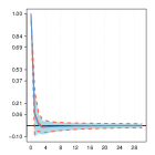
Gini

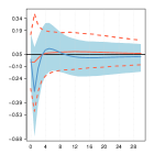
Real GDP

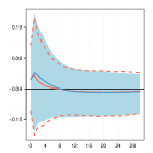
Infl. expect.

Unempl. rate

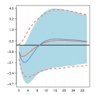
Long rates

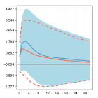
Real eff. exchange rate

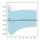
Equity prices

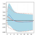
Path shock

Path shock

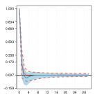
Gini

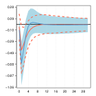
Real GDP

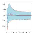
Infl. expect.

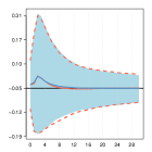
Unempl. rate

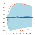
Long rates

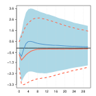
Real eff. exchange rate

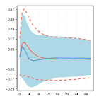
Equity prices

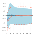
Notes: The plot shows results of a robustness exercise. In the top panel, we show structural responses to a one standard deviation increase in the target shock, in the bottom panel corresponding responses to a path shock. The derivation of these shocks is described in Kubota and Shintani (2020). For all plots, in blue, results are base on all households, in orange only for workers’ households. Posterior median along 68% credible sets. An increase in the real effective exchange rate corresponds to an appreciation.

Summing up, our main result namely that income inequality decreases when considering all households is robust to different identification schemes. The effect is less clear when considering workers’ households. This implies that the occupation of the household plays an important role when assessing the effects of monetary policy on income inequality. High-frequency identification suggests that most of the effect on the Gini comes from monetary policy that targets the long-end of the yield curve, i.e., quantitative easing policies. This suggests that the shadow rate seems to pick up these policies rather than conventional changes in the policy rate.

5 Conclusions

In this paper, we examine the relationship between monetary policy and income inequality in Japan. For that purpose, we propose a new framework that models jointly the volatility of the income distribution and the dynamics of key macroeconomic variables. Our model draws on relative frequencies of grouped income data which is continuously available over a longer period than comparable micro- / survey based individual income data, which makes it suitable to analyze with time series methods.

The empirical literature assessing monetary policy effects on income inequality has revealed a large degree of cross-country heterogeneity. This is the case since the theoretical effect is ambiguous and depends on the relative strength of transmission channels as well as endowments and demographics of households – all which might differ significantly across countries. Our analysis reveals that a monetary tightening in Japan leads to a decrease in output an increase in unemployment and an appreciation of the real effective exchange rate. We do not find any significant effects on (expected) inflation. As regards financial variables, we find that long-term rates respond positively to the tightening, whereas equity prices decrease significantly over the medium-term.

We then examine the effect o tightened monetary policy on income inequality as measured by changes in an estimated Gini coefficient. Our main finding is that a monetary tightening leads to a significant decrease in inequality if we consider a broad representation of income data that also includes the unemployed and retired population. More unemployment, potential lay-offs of exporting firms triggered by a real appreciation and tighter financing conditions tend to mostly affect the employed. In the broad household sample, this leads to a more equal income distribution. This finding is reversed, if we consider the sub-sample of households whose head is employed. Here tighter monetary policy leads to more inequality since the same effects now apply to the poorer population of the sample. This result is in line with recent findings of Coibion et al. (2017) for the USA, Mumtaz and Theophilopoulou (2017) for the UK and Furceri et al. (2017) for a broad set of countries. Using a counterfactual analysis reveals changes in long-term interest rates and – to a lesser degree – the unemployment rate as main drivers of inequality caused by monetary policy. Especially so for workers’ households, long-term rates which resemble overall financing conditions are crucial in transmitting monetary policy.

Compliance with Ethical Standards

Funding:

Kakamu acknowledges the financial support by KAKENHI (#16KK0081, #16K03592, #25245035, #20H00080 and #20K01590).

Conflict of Interest:

Author Feldkircher declares that he has no conflict of interest. Author Kakamu declares that he has no conflict of interest.

Ethical approval:

This article does not contain any studies with human participants or animals performed by any of the authors.

Appendix A Posterior Analysis

A.1 Sampling $\mu_{t}$ for $t=1,2,\ldots,T$

The full conditional distribution (FCD) of $\mu_{t}$ for $t=1,2,\ldots,T$ is given by

$$\mu_{t}|h_{t},\mathbf{x}_{t}\sim\mathcal{N}\left(\hat{\mu}_{t},\hat{\tau}_{t}^{2}\right),$$

where $\displaystyle\hat{\tau}_{t}^{2}=(\exp(-h_{t})\mathbf{1}_{k}^{\prime}{\mathbf{W}_{t}^{*}}^{-1}\mathbf{1}_{k}+\tau_{0}^{-2})^{-1}$, $\displaystyle\hat{\mu}_{t}=\hat{\tau}_{t}^{2}\left\{\exp(-h_{t})\mathbf{1}_{k}^{\prime}{\mathbf{W}_{t}^{*}}^{-1}\left(\ln\mathbf{x}_{t}-\exp(h_{t}/2)\mathbf{u}_{t}\right)+\tau_{0}^{-2}\mu_{0}\right\}$, and $\mathbf{1}_{k}$ is a $k\times 1$ unit vector.

A.2 Sampling $h_{t}$ for $t=1,2,\ldots,T$

$$\pi(h_{t}|\mu_{t},\text{\boldmath{$\alpha$}},\mathbf{B},\mathbf{\Sigma},\mathbf{h}_{-t},\mathbf{Y}^{*},\mathbf{x}_{t})\propto\exp(-h_{t}/2)\exp\left(-\frac{\mathbf{v}_{t}^{\prime}\mathbf{W}_{t}^{*-1}\mathbf{v}_{t}}{2\exp(h_{t})}\right)f(h_{t}),$$

where $\mathbf{h}_{-t}=(h_{1},h_{2},\ldots,h_{t-1},h_{t+1},\ldots,h_{T})$ and

$$f(h_{t})=\begin{cases}\displaystyle\exp\left(-\frac{\mathbf{e}_{t}^{\prime}\mathbf{\Sigma}^{-1}\mathbf{e}_{t}+\mathbf{e}_{t+1}^{\prime}\mathbf{\Sigma}^{-1}\mathbf{e}_{t+1}}{2}\right),&\text{if $t<T$}\\ \displaystyle\exp\left(-\frac{\mathbf{e}_{t}^{\prime}\mathbf{\Sigma}^{-1}\mathbf{e}_{t}}{2}\right),&\text{if $t=T$}\end{cases}.$$

In the sampling of $h_{t}$ for $t=1,2,\ldots,T$, we use normal distributions as the proposal distributions along with tuned random-walk procedures suggested by Holloway et al. (2002).

A.3 Sampling $\alpha$, $\mathbf{B}$ and $\mathbf{\Sigma}$

Let $\mathbf{y}=\text{vec}(\mathbf{Y})$ and $\mathbf{Z}=\left\{(\mathbf{I}_{m}\otimes(1,\mathbf{y}_{0}^{\prime}))^{\prime},(\mathbf{I}_{m}\otimes(1,\mathbf{y}_{1}^{\prime}))^{\prime},\ldots,(\mathbf{I}_{m}\otimes(1,\mathbf{y}_{T-1}^{\prime}))^{\prime}\right\}^{\prime}$, respectively, where $\mathbf{I}_{m}$ is an $m\times m$ unit matrix. Then,

$$\text{\boldmath{$\beta$}}|\mathbf{\Sigma},\mathbf{Y} \sim \mathcal{N}_{S}\left(\hat{\text{\boldmath{$\beta$}}},\hat{\mathbf{\Omega}}\right),$$

$$\mathbf{\Sigma}|\text{\boldmath{$\alpha$}},\mathbf{B},\mathbf{Y} \sim \mathcal{IW}\left(\hat{\nu},\hat{\mathbf{\Sigma}}\right)$$

where $\text{\boldmath{$\beta$}}=\text{vec}\left\{(\text{\boldmath{$\alpha$}},\mathbf{B})^{\prime}\right\}$, $S$ is the space, where $\mathbf{B}$ satisfies the stationary condition, $\hat{\mathbf{\Omega}}=\left\{\mathbf{Z}^{\prime}\left(\mathbf{I}_{T}\otimes\mathbf{\Sigma}^{-1}\right)\mathbf{Z}+\mathbf{\Omega}_{0}^{-1}\right\}^{-1}$, $\hat{\text{\boldmath{$\beta$}}}=\hat{\mathbf{\Omega}}\left\{\mathbf{Z}^{\prime}\left(\mathbf{I}_{T}\otimes\mathbf{\Sigma}^{-1}\right)\mathbf{y}+\mathbf{\Omega}_{0}^{-1}\text{\boldmath{$\beta$}}_{0}\right\}$, $\hat{\nu}=T+\nu_{0}$, $\hat{\mathbf{\Sigma}}=\mathbf{E}\mathbf{E}^{\prime}+\mathbf{\Sigma}_{0}$, and $\mathbf{E}=(\mathbf{e}_{1},\mathbf{e}_{2},\ldots,\mathbf{e}_{T})$.

References

- Altavilla et al. (2019) Altavilla C, Brugnolini L, Gürkaynak RS, Motto R, Ragusa G. 2019. Measuring euro area monetary policy. Journal of Monetary Economics 108: 162–179.
-
Amaral (2017)
Amaral PS. 2017.
Monetary Policy and Inequality.
Economic Commentary .
URL https://ideas.repec.org/a/fip/fedcec/00062.html - Bachmann and Sims (2012) Bachmann R, Sims E. 2012. Confidence and the transmission of government spending shocks. Journal of Monetary Economics 59: 235–249.
-
Baumeister and Benati (2013)
Baumeister C, Benati L. 2013.
Unconventional Monetary Policy and the Great Recession: Estimating
the Macroeconomic Effects of a Spread Compression at the Zero Lower Bound.
International Journal of Central Banking 9: 165–212.
URL https://ideas.repec.org/a/ijc/ijcjou/y2013q2a9.html - Bernanke (2017) Bernanke B. 2017. Some reflections on japanese monetary policy. Bank of Japan, May 24.
- Bernanke and Kuttner (2005) Bernanke BS, Kuttner KN. 2005. What explains the stock market’s reaction to federal reserve policy? Journal of Finance 60: 1221–1257.
- Bohl et al. (2017) Bohl M, Siklos PL, Werner T. 2017. Do Central Banks React to the Stock Market? The Case of the Bundesbank. Journal of Banking & Finance 31: 719–733.
- Carriero et al. (2018) Carriero A, Clark TE, Marcellino M. 2018. Measuring uncertainty and its impact on the economy. Review of Economics and Statistics 100: 799–815.
-
Chotikapanich et al. (2007a)
Chotikapanich D, Griffiths WE, Rao DSP. 2007a.
Estimating and combining national income distributions using limited
data.
Journal of Business & Economic Statistics 25:
97–109.
URL http://dx.doi.org/10.1198/073500106000000224 -
Chotikapanich et al. (2007b)
Chotikapanich D, Rao DSP, Tang KK. 2007b.
Estimating income inequality in China using grouped data and the
generalized beta distribution.
Review of Income and Wealth 53: 127–147.
ISSN 1475-4991.
URL http://dx.doi.org/10.1111/j.1475-4991.2007.00220.x - Christiano et al. (1999) Christiano LJ, Eichenbaum M, Evans CL. 1999. Monetary policy shocks: What have we learned and to what end? In Taylor JB, Woodford M (eds.) Handbook of Macroeconomics, volume 1 of Handbook of Macroeconomics, Elsevier, chapter 2. Elsevier, 65–148.
- Coibion et al. (2017) Coibion O, Gorodnichenko Y, Kueng L, Silvia J. 2017. Innocent bystanders? Monetary policy and inequality in the U.S. Journal of Monetary Economics 88: 70–89.
- Erosa and Ventura (2002) Erosa A, Ventura G. 2002. On inflation as a regressive consumption tax. Journal of Monetary Economics 49: 761–795.
-
Furceri et al. (2017)
Furceri D, Loungani P, Zdzienicka A. 2017.
The effects of monetary policy shocks on inequality.
Journal of International Money and Finance ISSN 0261-5606.
URL http://www.sciencedirect.com/science/article/pii/S0261560617302279 - Gertler and Karadi (2015) Gertler M, Karadi P. 2015. Monetary policy surprises, credit costs, and economic activity. American Economic Journal: Macroeconomics 7: 44–76.
-
Gornemann et al. (2012)
Gornemann N, Kuester K, Nakajima M. 2012.
Monetary policy with heterogeneous agents.
Working Papers 12-21, Federal Reserve Bank of Philadelphia.
URL https://ideas.repec.org/p/fip/fedpwp/12-21.html -
Holloway et al. (2002)
Holloway G, Shankar B, Rahman S. 2002.
Bayesian spatial probit estimation: a primer and an application to
hyv rice adoption.
Agricultural Economics 27: 383 – 402.
ISSN 0169-5150.
Spatial Analysis for Agricultural Economists: Concepts, Topics, Tools
and Examples.
URL http://www.sciencedirect.com/science/article/pii/S0169515002000701 - Honda and Kuroki (2006) Honda Y, Kuroki Y. 2006. Financial and capital markets’ responses to changes in the central bank’s target interest rate: The case of japan. The Economic Journal 116: 812–842.
-
Inui et al. (2017)
Inui M, Sudo N, Yamada T. 2017.
Effects of Monetary Policy Shocks on Inequality in Japan.
Bank of Japan Working Paper Series 17-E-3, Bank of Japan.
URL https://ideas.repec.org/p/boj/bojwps/wp17e03.html - Iwasaki and Sudo (2017) Iwasaki Y, Sudo N. 2017. Myths and Observations on Unconventional Monetary Policy: Takeaways from Post-Bubble Japan. Working paper No.17-E11, Bank of Japan.
- Jarociński and Karadi (2020) Jarociński M, Karadi P. 2020. Deconstructing monetary policy surprises—the role of information shocks. American Economic Journal: Macroeconomics 12: 1–43.
-
Kobayashi et al. (2021)
Kobayashi G, Yamauchi Y, Kakamu K, Kawakubo Y, Sugasawa S. 2021.
Bayesian approach to Lorenz curve using time series grouped data.
Journal of Business & Economic Statistics 0: 1–16.
URL https://doi.org/10.1080/07350015.2021.1883438 -
Kubota and Shintani (2020)
Kubota H, Shintani M. 2020.
High-frequency Identification of Unconventional Monetary Policy
Shocks in Japan.
CARF F-Series CARF-F-502, Center for Advanced Research in Finance,
Faculty of Economics, The University of Tokyo.
URL https://ideas.repec.org/p/cfi/fseres/cf502.html -
Li et al. (2010)
Li YD, Iscan TB, Xu K. 2010.
The impact of monetary policy shocks on stock prices: Evidence from
canada and the united states.
Journal of International Money and Finance 29:
876–896.
ISSN 0261-5606.
URL http://www.sciencedirect.com/science/article/pii/S0261560610000422 - Lise et al. (2014) Lise J, Sudo N, Suzuki M, Yamada K, Yamada T. 2014. Wage, Income and Consumption Inequality in Japan, 1981-2008: from Boom to Lost Decades. Review of Economic Dynamics 17: 582–612.
- Ludvigson et al. (2002) Ludvigson S, Steindel C, Lettau M. 2002. Monetary policy transmission through the consumption-wealth channel. Economic Policy Review : 410–423.
- McDonald and Ransom (2008) McDonald JB, Ransom M. 2008. The Generalized Beta Distribution as a Model for the Distribution of Income: Estimation of Related Measures of Inequality. New York, NY: Springer New York. ISBN 978-0-387-72796-7, 147–166.
- Miyao (2000) Miyao R. 2000. The Role of Monetary Policy in Japan: A Break in the 1990s? Journal of the Japanese and International Economies 14: 366–384.
- Miyao (2002) Miyao R. 2002. The Effects of Monetary Policy in Japan. Journal of Money, Credit and Banking 34: 367–392.
-
Mumtaz and Theophilopoulou (2017)
Mumtaz H, Theophilopoulou A. 2017.
The impact of monetary policy on inequality in the UK. An empirical
analysis.
European Economic Review 98: 117–133.
URL https://ideas.repec.org/a/fip/fednep/y2002imayp117-133nv.8no.1.html -
Nakajima et al. (2011)
Nakajima J, Kasuya M, Watanabe T. 2011.
Bayesian analysis of time-varying parameter vector autoregressive
model for the Japanese economy and monetary policy.
Journal of the Japanese and International Economies
25: 225–245.
URL https://ideas.repec.org/a/eee/jjieco/v25y2011i3p225-245.html - Nakashima et al. (2017) Nakashima K, Shibamoto M, Takahashi K. 2017. Identifying unconvetional monetary policy shocks. Discussion Paper Series DP2017-05, Kobe University.
- Nishino and Kakamu (2011) Nishino H, Kakamu K. 2011. Grouped data estimation and testing of Gini coefficients using lognormal distributions. Sankhya Series B 73: 193–210.
- Nishino and Kakamu (2015) Nishino H, Kakamu K. 2015. A random walk stochastic volatility model for income inequality. Japan and the World Economy 36: 21–28.
- Nishino et al. (2012) Nishino H, Kakamu K, Oga T. 2012. Bayesian estimation of persistent income inequality using the lognormal stochastic volatility model. Journal of Income Distribution 21: 88–101.
- Rigobon and Sack (2004) Rigobon R, Sack B. 2004. The impact of monetary policy on asset prices. Journal of Monetary Economics 51: 1553–1575.
- Saiki and Frost (2014) Saiki A, Frost J. 2014. Does unconventional monetary policy affect inequality? Evidence from Japan. Applied Economics 46: 4445–4454.
- Shirakawa (2010) Shirakawa M. 2010. Roles for a central bank–based on Japan’s experience of the bubble, the financial crisis, and deflation–. In Speech at the 2010 Fall Meeting of the Japan Society of Monetary Economics. Citeseer.
-
Spiegel and Tai (2018)
Spiegel MM, Tai A. 2018.
International transmission of japanese monetary shocks under low and
negative interest rates: A global factor-augmented vector autoregressive
approach.
Pacific Economic Review 23: 51–66.
URL https://onlinelibrary.wiley.com/doi/abs/10.1111/1468-0106.12252 - Thorbecke (1997) Thorbecke W. 1997. On stock market returns and monetary policy. Journal of Finance 52: 635–654.
-
Uhlig (2005)
Uhlig H. 2005.
What are the effects of monetary policy on output? Results from an
agnostic identification procedure.
Journal of Monetary Economics 52: 381–419.
URL https://ideas.repec.org/a/eee/moneco/v52y2005i2p381-419.html - Wong (2015) Wong B. 2015. Do Inflation Expectations Propagate the Inflationary Impact of Real Oil Price Shocks?: Evidence from the Michigan Survey. Journal of Money, Credit and Banking 47: 1673–1689.
-
Wu and Xia (2016)
Wu JC, Xia FD. 2016.
Measuring the macroeconomic impact of monetary policy at the zero
lower bound.
Journal of Money, Credit and Banking 48: 253–291.
ISSN 1538-4616.
URL http://dx.doi.org/10.1111/jmcb.12300