Fast swaption pricing in Gaussian term structure models

Abstract.

We propose a fast and accurate numerical method for pricing European swaptions in multi-factor Gaussian term structure models. Our method can be used to accelerate the calibration of such models to the volatility surface. The pricing of an interest rate option in such a model involves evaluating a multi-dimensional integral of the payoff of the claim on a domain where the payoff is positive. In our method, we approximate the exercise boundary of the state space by a hyperplane tangent to the maximum probability point on the boundary and simplify the multi-dimensional integration into an analytical form. The maximum probability point can be determined using the gradient descent method. We demonstrate that our method is superior to previous methods by comparing the results to the price obtained by numerical integration.

1. Introduction

Swaptions, which are options on interest rate swaps, are the simplest and most liquid option products traded in fixed income markets. From practical and theoretical perspectives, swaptions are important building blocks for more complicated claims, such as Bermudan callable swaps. Swaptions are traded to hedge the volatility risk of such exotic claims. Therefore, the parameters of a term structure model must be calibrated to exactly reproduce the prices of the swaptions observed in the market before they are used to price exotic claims. However, the calibration process is typically a nonlinear multi-dimensional root solving problem for which parameters must be found using iterative methods. Therefore, it is critical to have a fast and reliable method to price swaptions given a set of parameters for a term structure model.

The most relevant studies on this topic are by Singleton and Umantsev (2002) and Schrager and Pelsser (2006). Both studies provide a fast pricing method for the class of affine term structure models (ATSM). Singleton and Umantsev (2002) observe that the non-linear exercise boundary for swaptions can be approximated by a hyperplane. They compute the probability over the approximated domain using the transform inversion method developed by Duffie et al. (2000) and Bakshi and Madan (2000). Schrager and Pelsser (2006) derive an approximated stochastic differential equation (SDE) for the underlying swap rate from full interest rate dynamics, from which the swaption price is easily obtained. They assume that the low variance martingale (LVM), which is typically the ratio of the discount factors, is constant as time-zero value. Andersen and Piterbarg (2010c) further refine the method by improving the estimation of LVMs. Because of its easy and intuitive implementation, the Schrager and Pelsser (2006) method has been favored by practitioners. Considering that the method of freezing LVMs is inspired by a similar method for pricing swaptions in the LIBOR Market Model (LMM), their method is arguably the dominant swaption pricing method for all classes of interest rates term structure models. Although the Singleton and Umantsev (2002) method appears to be equally promising, it suffers from several drawbacks. First, because it lacks explicit guidance in selecting the hyperplane, it fails to provide the best hyperplane to minimize the error. Second, even for a given hyperplane, the probability over the region must be computed under different forward measures; there are as many measures as the number of cash flows of the underlying swaptions.

This study demonstrates that the hyperplane approximation can be significantly improved for the class of Gaussian term structure models (GTSM). Using the analytical tractability of the GTSM, we can overcome the two drawbacks mentioned above. In the GTSM, the probability density function of the state is simply a multivariate Gaussian. In other words, the GTSM is similar to the ATSM, where the transform inversion is analytically solved. The knowledge of the density function enables us to find the best hyperplane to approximate the non-linear boundary. We identify the point on the boundary with the maximum probability density and determine the hyperplane tangent at that point.

The accuracy of our approximation is better than the accuracy of previous methods by several orders of magnitude, regardless of the moneyness, expiry and tenor of the swaptions. Moreover, our method does not sacrifice computational cost. The computational cost grows at most linearly with the number of factors of the GTSM. Although our method is limited to the GTSM, which is a subset of the ATSM, it is still a significant improvement for swaption calibration given the indisputable importance of the GTSM among all term structure models. Several previous term structure models are special cases of the GTSM, e.g., Ho and Lee (1986), Hull and White (1990) and Vasicek (1977). These models are still used by practitioners in their extended forms. In the GTSM, we have the added benefit of being able to compare our approximation to the exact swaption price. In contrast to the general ATSM, where it is necessary to resort to Monte Carlo simulations, we can obtain the exact price by combining the analytical result with numerical integration. Thus, we can provide an accurate error analysis.

The remainder of the paper is organized as follows. In Section 2, we briefly review the Gaussian term structure model. Section 3 describes the hyperplane approximation method and the exact swaption pricing. Section 4 demonstrates the accuracy of our method and compares it to previous methods.

2. Multi-factor Gaussian term structure model

In this section, we review the important results of the GTSM. We will define the scope of the GTSM and describe the preconditions for which our approximation method is valid. To simplify notation, define an element-wise multiplication operator, $\circ$ , between vectors or between a vector and a matrix by

(2.1) $$\mathbf{a}\circ\mathbf{b}=\mathbf{b}\circ\mathbf{a}=\big{[}\;a_{j}b_{j}\;\big{]}_{j}\;,$$

(2.2) $$\mathrm{M}\circ\mathbf{a}=\mathbf{a}\circ\mathrm{M}=\big{[}\;M_{jk}a_{j}\;\big{]}_{j,\,k}\;,$$

(2.3) $$\text{and}\quad\mathrm{M}\circ\mathbf{a}^{\top}=\mathbf{a}^{\top}\circ\mathrm{M}=\big{[}\;M_{jk}a_{k}\;\big{]}_{j,\,k}\;,$$

where $\mathbf{a}=[a_{j}]_{j}$ and $\mathbf{b}=[b_{j}]_{j}$ are $d\times 1$ vectors and $\mathrm{M}=[M_{jk}]_{j,\,k}$ is a $d\times d$ matrix.

The GTSM in this study is a subclass of the Heath-Jarrow-Morton (HJM) model class (Heath et al., 1992). A general $d$-dimension HJM model starts with the dynamics of the price of a zero-coupon bond. Let $P(t,T)$ be the time-$t$ price of a zero-coupon bond maturing at $T$ and let the SDE be defined as follows:

(2.4) $$\frac{dP(t,T)}{P(t,T)}=r(t)\,dt-\boldsymbol{\sigma}_{P}(t,T)^{\top}d\mathbf{W}^{\beta}(t),$$

where $r(t)$ is the short rate process; $-\boldsymbol{\sigma}_{P}(t,T)$ is the volatility vector; and $\mathbf{W}^{\beta}(t)$ is a $d$-dimensional Brownian motion under the risk-neutral measure $Q^{\beta}$. The components of $\mathbf{W}^{\beta}(t)$ are correlated with a correlation matrix $\mathrm{R}(t)=\left[\,\rho_{jk}(t)\,\right]_{j,\,k}$ where $\rho_{kk}(t)=1$. If $f(t,T)$ is the instantaneous forward rate (IFR) for time $T$ observed at the current time $t$, we can write $P(t,T)=\exp\left(-\int_{t}^{T}f(t,\,s)\;ds\right)$. An important result of the HJM model is obtained by inserting this equation into the SDE for $P(t,T)$, to show that

(2.5) $$df(t,T)=\boldsymbol{\sigma}_{f}(t,T)^{\top}\boldsymbol{\sigma}_{P}(t,T)\,dt+\boldsymbol{\sigma}_{f}(t,T)^{\top}d\mathbf{W}^{\beta}(t),$$

where the volatility of IFR $\boldsymbol{\sigma}_{f}(t,T)$ is as follows:

(2.6) $$\boldsymbol{\sigma}_{f}(t,T)=\frac{\partial}{\partial T}\,\boldsymbol{\sigma}_{P}(t,T).$$

Furthermore, the short rate process $r(t)$ is

(2.7) $$r(t)=f(t,t)=f(0,t)+\mathbf{1}^{\top}\mathbf{x}(t),$$

for a $d\times 1$ state vector process $\mathbf{x}(t)$ with $\mathbf{x}(0)=0$ and

(2.8) $$\mathbf{x}(t)=\int_{0}^{t}\boldsymbol{\sigma}_{f}(s,t)\circ\int_{s}^{t}\boldsymbol{\sigma}_{f}(s,u)\;du\,ds+\int_{0}^{t}\boldsymbol{\sigma}_{f}(s,t)\circ d\mathbf{W}^{\beta}(s).$$

We can further simplify the result under the $t$-forward measure $Q^{t}$. Using the Girsanov theorem, we obtain

(2.9) $$d\mathbf{W}^{\beta}(s)=d\mathbf{W}^{t}(s)-\boldsymbol{\sigma}_{P}(s,t)ds=d\mathbf{W}^{t}(s)-\int_{s}^{t}\boldsymbol{\sigma}_{f}(s,u)\,du\;ds,$$

where $\mathbf{W}^{t}(\cdot)$ is the Brownian motion under the $Q^{t}$ measure. The processes for $f(s,t)$ and $\mathbf{x}(s)$ with respect to the time $s$ become driftless

(2.10) $$df(s,t)=\boldsymbol{\sigma}_{f}(s,t)^{\top}d\mathbf{W}^{t}(s)\quad\text{and}\quad\mathbf{x}(t)=\int_{0}^{t}\boldsymbol{\sigma}_{f}(s,t)\circ d\mathbf{W}^{t}(s).$$

This result is consistent with the intuitive observation that $f(s,t)$ is a Martingale under the $Q^{t}$ measure with respect to time $s$.

An important result from Heath et al. (1992) is that, given the interest rate curve $f(0,T)$ as an input to the model, the diffusion of the interest rate curve is fully defined by specifying the volatility $\boldsymbol{\sigma}_{f}(t,T)$. However, an HJM model typically imposes restrictions on $\boldsymbol{\sigma}_{f}(t,T)$ because the process is generally path-dependent or non-Markovian.

It is known that an HJM model is Markovian if and only if the $\boldsymbol{\sigma}_{f}(t,T)$ is deterministic and separable in the form of $\mathrm{G}(T)\mathbf{h}(t)$ for a $d\times d$ matrix $\mathrm{G}(T)$ and a $d\times 1$ vector $\mathbf{h}(t)$ (Andersen and Piterbarg, 2010a). Based on this assumption, the IFR $f(t,T)$ and the state vector $\mathbf{x}(t)$ are also Gaussian.

Although it is not a necessary condition for this study, a popular choice for a separable form of $\boldsymbol{\sigma}_{f}$ is one that causes the short rate $r(t)$ to follow a mean-reverting Ornstein-Uhlenbeck process,

(2.11) $$d\mathbf{x}(t)=(\Pi(t)\mathbf{1}-\boldsymbol{\lambda}(t)\circ\mathbf{x}(t))dt+\boldsymbol{\sigma}_{r}(t)^{\top}d\mathbf{W}^{\beta}(t)$$

for a deterministic mean reversion coefficient $\boldsymbol{\lambda}(t)$, a deterministic short rate volatility vector $\boldsymbol{\sigma}_{r}(t)$ and a drift matrix $\Pi(t)$. This choice is equivalent to setting

(2.12) $$\boldsymbol{\sigma}_{f}(t,T)=\boldsymbol{\sigma}_{r}(t)\circ\mathbf{m}(t,T),$$

where $\mathbf{m}(t,T)$ is the exponential decay factor between time $t$ and $T$, defined by

(2.13) $$\mathbf{m}(t,T)=\left[\;e^{-\int_{t}^{T}\lambda_{k}(s)ds}\;\right]_{k}\quad\text{for}\quad\boldsymbol{\lambda}(t)=\Big{[}\;\lambda_{k}(t)\;\Big{]}_{k}\;.$$

The state $\mathbf{x}(t)$ is multivariate Gaussian. The drift matrix $\Pi(t)$ is the covariance matrix of $\mathbf{x}(t)$. From Eq. (2.10), we obtain

(2.14) $$\Pi(t) =\int_{0}^{t}(\boldsymbol{\sigma}_{f}(s,t)\circ d\mathbf{W}^{t}(s))\,(\boldsymbol{\sigma}_{f}(s,t)\circ d\mathbf{W}^{t}(s))^{\top}$$

$$=\int_{0}^{t}\boldsymbol{\sigma}_{r}(s)\circ\mathbf{m}(s,t)\circ\mathrm{R}(s)\circ\boldsymbol{\sigma}_{r}(s)^{\top}\circ\mathbf{m}(s,t)^{\top}ds\,$$

$$=\left[\int_{0}^{t}\rho_{jk}(t)\sigma_{rj}(s)\sigma_{rk}(s)m_{j}(s,t)m_{k}(s,t)\;ds\right]_{j,\,k}.$$

Finally, we can reconstruct the zero-coupon bond price at the future time $t$ using the Markovian state $\mathbf{x}(t)$ as

(2.15) $$P(t,T)=\frac{P(0,T)}{P(0,t)}\exp\left(-\mathbf{g}(t,T)^{\top}\mathbf{x}(t)-\frac{1}{2}\,\mathbf{g}(t,T)^{\top}\Pi(t)\>\mathbf{g}(t,T)\right),$$

where $\mathbf{g}(t,T)=\int_{t}^{T}\mathbf{m}(t,s)\,ds$. The volatility of $P(t,T)$ is conveniently given as $\boldsymbol{\sigma}_{P}(t,T)=-\boldsymbol{\sigma}_{r}(t)\circ\mathbf{g}(t,T)$; thus, $\mathbf{g}(t,T)$ is the risk loading of the zero-coupon bond with respect to the short rate volatility. It should be noted that under the $t$-forward measure, $\mathbf{x}(t)$ has a zero mean, and $E^{Q^{t}}\{P(t,T)\}=P(0,T)/P(0,t)$. This result is consistent with the fact that $P(s,T)/P(s,t)$ is a Martingale with respect to time $s$ under the $Q^{t}$ measure.

3. Swaption pricing method

Here, we derive the price of a swaption using the result from the previous section. Let us assume that the underlying swap of a swaption begins at a forward time $T_{0}$, pays the fixed coupon $K$ (payer swap) on a payment schedule $\{T_{1},\cdots T_{m}\}$, and receives the floating interest rate, typically LIBOR. The value of this underlying swap, at time $t$, is

(3.1) $$\text{V}(t)=P(t,T_{0})-P(t,T_{m})-\sum_{k=1}^{m}KP(t,T_{k})\Delta_{k},$$

where $\Delta_{k}$ is the day count fraction for the $k$-th period, $\Delta_{k}=T_{k}-T_{k-1}$. In general,

(3.2) $$\text{V}(t)=\sum_{k=0}^{m}P(t,T_{k})\,\text{CF}(T_{k}),$$

for the cash flow series $\text{CF}(T_{k})$ at time $T_{k}$.

Let $T_{e}$ be the expiry of the swaption to enter into the underlying swap paying the fixed coupon $K$ (the expiry $T_{e}$ is typically two business days before the start of the swap $T_{0}$). Using the reconstruction formula Eq. (2.15), we can express the future value of the swap as a function of the state $\mathbf{x}(T_{e})$.

We first decorrelate and normalize the state variable $\mathbf{x}(t)$ into $\mathbf{z}(t)$ by $\mathbf{x}(t)=C(t)\;\mathbf{z}(t)$ for a Cholesky decomposition, $\mathrm{C}(t)$, of the covariance matrix $\Pi(t)$ that satisfies $\Pi(t)=\mathrm{C}(t)\,\mathrm{C}(t)^{\top}$. Then, the reconstruction formula becomes

(3.3) $$P(t,T)=\frac{P(0,T)}{P(0,t)}\exp\left(-\mathbf{a}(t,T)^{\top}\,\mathbf{z}(t)-\frac{1}{2}\,|\mathbf{a}(t,T)|^{2}\right).$$

where $\mathbf{a}(t,T)=\mathrm{C}(t)^{\top}\,\mathbf{g}(t,T)$.

We now have the value of the swap at the expiry $T_{e}$ as a function of the state $\mathbf{z}=\mathbf{z}(T_{e})$

(3.4) $$V(\mathbf{z})=\frac{1}{P(0,T_{e})}\;\sum_{k=0}^{m}\text{DCF}_{k}\;\exp\left(-\mathbf{a}_{k}^{\top}\mathbf{z}-\frac{1}{2}\,|\mathbf{a}_{k}|^{2}\right)$$

where $\text{DCF}_{k}$ is the discounted cash flow $\text{CF}(T_{k})P(0,T_{k})$, and $\mathbf{a}_{k}=\mathbf{a}(T_{e},T_{k})$. The price of the payer swaption is the expectation of $V(\mathbf{z})$ under the $T_{e}$-forward measure,

(3.5) $$C=P(0,T_{e})\;E^{Q^{T_{e}}}\left\{\;\max(V(\mathbf{z}),0)\;\right\}.$$

Similarly, the $T_{e}$-forward price of the receiver swaption is given by

(3.6) $$P=P(0,T_{e})\;E^{Q^{T_{e}}}\left\{\;\max(-V(\mathbf{z}),0)\;\right\}.$$

The remainder of this study focuses on the payer swaption. The receiver swaption can be determined from the put-call parity relation.

3.1. Hyperplane approximation

The evaluation of Eq. (3.5) involves a $d$-dimensional integration. The difficulty lies in identifying the integration domain $\Omega$, where the underlying swap has a positive value and the boundary $\partial\Omega$ can be given as

(3.7) $$\Omega=\{\mathbf{z}:\;V(\mathbf{z})\geq 0\},\quad\partial\Omega=\{\mathbf{z}:\;V(\mathbf{z})=0\}.$$

As described by Singleton and Umantsev (2002), we simplify the integration by approximating the boundary $\partial\Omega$ as a hyperplane. However, in this study, we substantially refine the original idea by providing a systematic way to determine the best hyperplane to use for this approximation.

At the exercise boundary, we identify the state $\mathbf{z}^{*}$ with the maximum probability density. Then, for the approximation, we use the tangent plane to the boundary at $\mathbf{z}^{*}$, which is a systematic way of choosing the hyperplane without ad-hoc rules based on experience. This technique can be applied to any moneyness of swaptions and any dimension of the GTSM. Because $\mathbf{z}$ has an uncorrelated multivariate normal distribution, the probability density decreases as a function of $|\mathbf{z}|$. Thus, $\mathbf{z}^{*}$ is also the point with the shortest distance to the origin $\boldsymbol{0}$ among the points on the boundary $\partial\Omega$. Furthermore, it follows that $\mathbf{z}^{*}$ should be a scalar multiple of $\boldsymbol{\nabla}V(\mathbf{z}^{*})$. We will use this property to find $\mathbf{z}^{*}$. See Figure 1 for a geometric illustration.

The point $\mathbf{z}^{*}$ can be found numerically using the following iterative method. One iteration consists of the following two steps: from $\mathbf{z}^{(i)}$ to $\mathbf{z}^{(i+\frac{1}{2})}$ and from $\mathbf{z}^{(i+\frac{1}{2})}$ to $\mathbf{z}^{(i+1)}$.

(1):

First, apply a step of steepest descent method from $\mathbf{z}^{(i)}$:

(3.8) $$\mathbf{z}^{(i+\frac{1}{2})}=\mathbf{z}^{(i)}-\frac{V(\mathbf{z}^{(i)})}{|\boldsymbol{\nabla}V(\mathbf{z}^{(i)})|^{2}}\boldsymbol{\nabla}V(\mathbf{z}^{(i)})$$

(2):

Then, project $\mathbf{z}^{(i+\frac{1}{2})}$ onto the gradient direction $\boldsymbol{\nabla}V(\mathbf{z}^{(i+\frac{1}{2})})$ by

(3.9) $$\mathbf{z}^{(i+1)}=\frac{\boldsymbol{\nabla}V(\mathbf{z}^{(i+\frac{1}{2})})^{\top}\mathbf{z}^{(i+\frac{1}{2})}}{|\boldsymbol{\nabla}V(\mathbf{z}^{(i+\frac{1}{2})})|^{2}}\;\boldsymbol{\nabla}V(\mathbf{z}^{(i+\frac{1}{2})}).$$

The convergence to the root is satisfied when the error $V(\mathbf{z}^{(i+1)})$ is below a certain threshold; we use $10^{-13}$ in our study.

It is difficult to prove with mathematical rigor that the iterative scheme converges to a root for all possible parameterizations. However, our method works without failure for any reasonable parameterization. In the GTSM, the state variable is proportional to the interest rate as a leading order, even allowing negative interest rates. Thus, it is possible to find a state $\mathbf{z}$ for which the swap rate is equal to any given (even negative) strike, which ensures that a boundary $\partial\Omega$ always exists and is close to a hyperplane. This iterative root-finding process uses the most time in the entire computation of the swaption price because the rest of the computation is analytical. A reasonably calibrated GTSM converges to the root $\mathbf{z}^{*}$ quickly, typically within 7 iterations starting from the origin. It should be noted that the number of iterations does not increase with the dimension $d$, although the computational cost may increase due to the increasing number of components. Overall, the computation cost increases linearly, not exponentially, with the dimension $d$.

Now, we can simplify the evaluation of Eq. (3.5). Let $\mathbf{q}_{1}=\boldsymbol{\nabla}V(\mathbf{z}^{*})/|\boldsymbol{\nabla}V(\mathbf{z}^{*})|$ be the unit vector in the direction of $\boldsymbol{\nabla}V(\mathbf{z}^{*})$. We express the state vector as follows:

(3.10) $$\mathbf{z}=y_{1}\,\mathbf{q}_{1}+\cdots+y_{d}\,\mathbf{q}_{d}$$

in a Cartesian coordinate $\mathbf{y}=(y_{1},\cdots,y_{d})$ with the standard basis $\{\mathbf{q}_{1},\cdots,\mathbf{q}_{d}\}$. The unspecified unit vectors $\mathbf{q}_{2},\cdots,\mathbf{q}_{d}$ can be chosen arbitrarily as long as the matrix of unit vectors $\mathrm{Q}=\big{[}\,\mathbf{q}_{1},\cdots,\mathbf{q}_{d}\,\big{]}$ forms an orthogonal matrix.

Using the above property, we select a scalar $d^{*}$ and vectors $\mathbf{b}_{k}$ such that

(3.11) $$\mathbf{z}^{*}=d^{*}\,\mathbf{q}_{1},\qquad\mathbf{a}_{k}=\mathrm{Q}\,\mathbf{b}_{k}$$

The approximated domain $\tilde{\Omega}$ is

(3.12) $$\tilde{\Omega}=\{\mathbf{z}:\;\mathbf{q}_{1}^{\top}(\mathbf{z}-\mathbf{z}^{*})\geq 0\}=\{\mathbf{y}:\;y_{1}\geq d^{*}\}$$

and the value of the swap becomes

(3.13) $$V(\mathbf{z})=\frac{1}{P(0,T_{e})}\;\sum_{k=0}^{m}\text{DCF}_{k}\exp\left(-\frac{1}{2}\,|\mathbf{b}_{k}|^{2}-\mathbf{b}_{k}^{\top}\,\mathbf{y}\right)$$

When integrating on the $\mathbf{y}$ coordinate, $y_{1}$ is the only axis on which the integration is non-trivial. The rest of the dimensions integrate to unity. We obtain the swaption price in analytic form as follows:

(3.14) $$C =P(0,T_{e})\,\int_{\Omega}V(\mathbf{z})f(\mathbf{z})\;d\mathbf{z}\approx P(0,T_{e})\,\int_{\tilde{\Omega}}V(\mathbf{y})f(\mathbf{y})\;d\mathbf{y}$$

$$=\sum_{k=0}^{m}\text{DCF}_{k}\int_{-\infty}^{\infty}\!\!dy_{2}\cdots dy_{d}\int_{d^{*}}^{\infty}\!\!dy_{1}\;\;e^{-\frac{1}{2}\,|\mathbf{b}_{k}|^{2}-\sum_{j=1}^{d}b_{kj}y_{j}}n(y_{1})\cdots n(y_{d})$$

$$=\sum_{k=0}^{m}\text{DCF}_{k}\int_{d^{*}}^{\infty}\!\!dy_{1}\;\;e^{-\frac{1}{2}\,b_{k1}^{2}-b_{k1}y_{1}}n(y_{1})$$

$$=\sum_{k=0}^{m}\text{DCF}_{k}\;N(-b_{k1}-d^{*})=\sum_{k=0}^{m}\text{DCF}_{k}\;N(-(\mathbf{a}_{k}+\mathbf{z}^{*})^{\top}\mathbf{q}_{1}),$$

where $f(\cdot)$ is the probability density function of the multivariate normal distribution, and $n(\cdot)$ and $N(\cdot)$ are the probability and cumulative density functions of the univariate normal distribution, respectively.

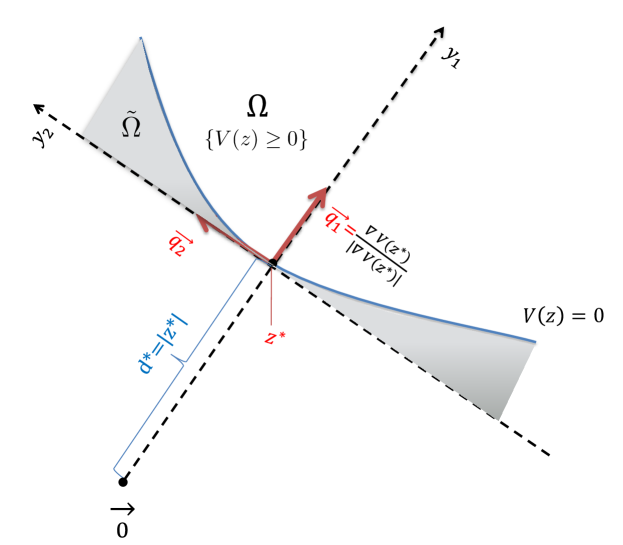
Figure 1. Schematic of the hyperplane approximation method. The domain of state variables, $\Omega$, includes the area where the swaption payoff is in the money. We approximate the boundary of $\Omega$, $\partial\Omega$, as a hyperplane tangent ($y_{1}=0$) to the point $\mathbf{z}^{*}$ where the probability density is maximal on $\partial\Omega$ and integrate the payoff over the domain above the hyperplane ($y_{1}\geq 0$). Therefore, the integration over the shaded area is incorrectly added to our approximation. However, the error is extremely small, as the swaption payoff is close to zero, and the probability density is small because of the choice of the tangent point, $\mathbf{z}^{*}$.

3.2. Exact pricing method

Although it is computationally demanding, we can combine numerical integration and analysis to price the swaption precisely and measure the accuracy of the hyperplane approximation. The integration is performed on the $\mathbf{y}$ coordinate, i.e., in the hyperplane approximation. However, in the exact method, we numerically determine the distance to the boundary $d$ for each given $(d\!-\!1)$-tuple $(y_{2},\cdots,y_{d})$:

(3.15) $$\Omega=\{\mathbf{y}:\;y_{1}\geq d(y_{2},\cdots,y_{d})\}.$$

The root finding for $d$ can be determined using the Newton-Raphson method in one-dimension. The integration is performed analytically for $y_{1}$ and numerically for the rest of the dimensions:

(3.16) $$C =P(0,T_{e})\,\int_{\Omega}V(\mathbf{z})f(\mathbf{z})\;d\mathbf{z}=P(0,T_{e})\,\int_{\Omega}V(\mathbf{y})f(\mathbf{y})\;d\mathbf{y}$$

$$=\sum_{k=0}^{m}\text{DCF}_{k}\int_{-\infty}^{\infty}\!\!dy_{2}\cdots dy_{d}\int_{d}^{\infty}\!\!dy_{1}\;e^{-\frac{1}{2}\,|\mathbf{b}_{k}|^{2}-\sum_{j=1}^{d}b_{kj}y_{j}}n(y_{1})\cdots n(y_{d})$$

$$=\sum_{k=0}^{m}\text{DCF}_{k}\int_{-\infty}^{\infty}\!\!dy_{2}\cdots dy_{d}\;\;N(-b_{k1}-d(y_{2},\cdots,y_{d}))n(y_{2}+b_{k2})\cdots n(y_{d}+b_{kd})$$

We can use the finite difference method for the numerical integration.

It should be noted that the error from the hyperplane approximation is due to the difference between the integrands of Eq. (3.14) and Eq. (3.16):

(3.17) $$E(y_{2},\cdots,y_{d})=\sum_{k=0}^{m}\left(N(-b_{k1}-d^{*})-N(-b_{k1}-d(\cdots))\right)n(y_{2}+b_{k2})\,\cdots\,n(y_{d}+b_{kd})$$

We will examine this error through examples in the next section. It is interpreted as the error density because the error in the swaption price is

(3.18) $$\text{Price Error}=\int_{-\infty}^{\infty}\!\!dy_{2}\cdots dy_{d}\;E(y_{2},\cdots,y_{d})$$

4. Approximation quality and comparison to other methods

To examine the quality of the proposed hyperplane approximation method for swaption pricing, we apply it to three sets of examples, shown in Table 1 to Table 3. The first two examples use different parameter sets in a two-factor GTSM calibrated to realistic swaption volatility surfaces in the least-square sense. We select two contrasting market conditions in the shapes of the yield curve and the volatility surface to test our approximation in diverse market environments. In the first example, the market sees high uncertainty in the short-term interest rate, and the yield curve is flat at $5\%$ at time 0. In the second example, the market sees high uncertainty in the long-term interest rate, and the interest rate curve increases steeply from the $0\%$ short-term interest rate, most likely because of monetary policies.

To calibrate the surface as closely as possible, we use a piece-wise-constant term structure for volatility and a mean reversion structure for the first factor with Parameter Sets 1 and 2. The parameters for the second factor are specified through the constant volatility ratio $\sigma_{2}/\sigma_{1}$ and the constant mean reversion difference $\lambda_{2}-\lambda_{1}$. This structure allows the instantaneous correlation between $f(t,T_{1})$ and $f(t,T_{2})$ to be stationary (Andersen and Piterbarg, 2010b).

For the third example, we reuse the three-factor GTSM parameter set from Collin-Dufresne and Goldstein (2002). This parameter set was also used by Schrager and Pelsser (2006) to compare their result to those of Collin-Dufresne and Goldstein (2002).

Table 1. Parameter Set 1: A two-factor Gaussian model calibrated to a volatility surface, where the swaptions on the shorter tenor swaps are relatively expensive. The current forward rate curve is assumed to be flat at $5\%$.

Time(year)	0 $\sim$ 0.25	$\sim$ 0.5	$\sim$ 1	$\sim$ 2	$\sim$ 5	$\sim$
Volatility($\sigma_{1}$)	0.030	0.024	0.024	0.022	0.018	0.012
Time(year)	0 $\sim$ 5		$\sim$ 10		$\sim$
Mean reversion($\lambda_{1}$)	0.115		0.073		0.029
$\sigma_{2}/\sigma_{1}$	1.05
$\lambda_{2}-\lambda_{1}$	0.27
$\rho_{12}$	-77%
$f(0,t)$	5%

Table 2. Parameter Set 2: A two-factor Gaussian model calibrated to a volatility surface where the swaptions on the longer tenor swaps are relatively expensive. The current forward rate curve is assumed to increase steeply from $0\%$ to $6\%$.

Time(year)	0 $\sim$ 0.25	$\sim$ 0.5	$\sim$ 1	$\sim$ 2	$\sim$ 5	$\sim$
Volatility($\sigma_{1}$)	0.020	0.014	0.013	0.012	0.01	0.009
Time(year)	0 $\sim$ 5		$\sim$ 10		$\sim$
Mean reversion($\lambda_{1}$)	-0.051		0.059		0.017
$\sigma_{2}/\sigma_{1}$	1.05
$\lambda_{2}-\lambda_{1}$	0.27
$\rho_{12}$	-77%
$f(0,t)$	6%$\times(1-e^{-t/10})$

Table 3. Parameter Set 3: A three-factor Gaussian model from Collin-Dufresne and Goldstein (2002) and Schrager and Pelsser (2006)

$\sigma_{1}$	$\sigma_{2}$	$\sigma_{3}$	$\lambda_{1}$	$\lambda_{2}$	$\lambda_{3}$	$\rho_{12}$	$\rho_{13}$	$\rho_{23}$	$f(0,t)$
0.010	0.005	0.002	1.0	0.2	0.5	-20%	-10%	30%	5.5%

Table 4. Prices and errors of the hyperplane approximation with Parameter Set 1 in basis point units. Relative pricing errors, calculated as fractions of exact prices, are in parentheses.

option	swap maturity
expiry	1	2	5	10	30
ATM	$K=F$
1	54.54 (-9.1E-12)	100.91 (-2.4E-09)	213.22 (-1.0E-06)	346.39 (-2.5E-05)	572.21 (-5.0E-04)
2	65.39 (-9.8E-12)	122.63 (-2.6E-09)	264.82 (-1.1E-06)	435.98 (-2.8E-05)	729.43 (-5.9E-04)
5	71.55 (-5.0E-12)	137.82 (-1.1E-09)	308.60 (-5.3E-07)	525.22 (-1.8E-05)	898.62 (-4.2E-04)
10	62.45 (-9.5E-13)	122.06 (-2.3E-10)	283.69 (-1.4E-07)	493.42 (-5.6E-06)	842.60 (-1.5E-04)
20	50.97 (-6.0E-13)	99.08 (-1.4E-10)	227.00 (-9.0E-08)	389.08 (-3.8E-06)	651.58 (-1.1E-04)
ITM	$K=F-\sigma_{\text{\tiny ATM}}\sqrt{T_{e}}$
1	147.97 (-2.2E-12)	273.77 (-7.6E-10)	578.43 (-3.4E-07)	939.35 (-8.9E-06)	1547.59 ( -1.9E-04)
2	177.39 (-2.6E-12)	332.63 (-6.4E-10)	718.27 (-2.9E-07)	1181.97 (-7.9E-06)	1970.51 (-1.9E-04)
5	194.04 (-4.9E-13)	373.76 (-1.9E-10)	836.80 (-9.6E-08)	1423.69 (-3.4E-06)	2423.75 (-9.5E-05)
10	169.34 (2.4E-13)	330.98 (-3.0E-11)	769.25 (-1.9E-08)	1337.53 (-7.5E-07)	2269.43 ( -2.6E-05)
20	138.14 (6.1E-13)	268.53 (-6.7E-12)	615.15 (-4.9E-09)	1053.67 (-2.3E-07)	1749.22 (-1.2E-05)
OTM	$K=F+\sigma_{\text{\tiny ATM}}\sqrt{T_{e}}$
1	11.51 (-7.7E-12)	21.31 (-2.4E-09)	45.09 (-9.6E-07)	73.60 (-2.3E-05)	125.63 (-4.3E-04)
2	13.84 (-1.1E-11)	25.97 (-2.9E-09)	56.15 (-1.2E-06)	93.00 (-2.9E-05)	162.31 (-5.7E-04)
5	15.20 (-5.8E-12)	29.28 (-1.5E-09)	65.66 (-6.7E-07)	112.24 (-2.2E-05)	203.21 (-4.8E-04)
10	13.29 (-1.5E-12)	25.97 (-3.3E-10)	60.34 (-2.0E-07)	105.39 (-8.0E-06)	193.21 (-1.9E-04)
20	10.92 (-6.2E-13)	21.22 (-2.4E-10)	48.67 (-1.6E-07)	84.12 (-6.5E-06)	154.65 (-1.6E-04)

Table 5. Implied normal volatilities and errors of the hyperplane approximation with Parameter Set 1 in daily basis point units. Relative volatility errors, calculated as fractions of exact volatilities, are in parentheses.

option	swap maturity
expiry	1	2	5	10	30
ATM	$K=F$
1	9.45 (-1.6E-12)	8.96 (-2.1E-10)	8.14 (-3.8E-08)	7.44 (-5.4E-07)	6.22 (-5.4E-06)
2	8.40 (-1.3E-12)	8.07 (-1.7E-10)	7.50 (-3.0E-08)	6.94 (-4.4E-07)	5.88 (-4.7E-06)
5	6.74 (-4.7E-13)	6.66 (-5.5E-11)	6.41 (-1.1E-08)	6.13 (-2.1E-07)	5.32 (-2.5E-06)
10	5.34 (-8.3E-14)	5.35 (-1.0E-11)	5.35 (-2.7E-09)	5.23 (-5.9E-08)	4.52 (-8.1E-07)
20	5.08 (-6.0E-14)	5.06 (-6.9E-12)	4.9 (-2.0E-09)	4.81 (-4.7E-08)	4.08 (-6.9E-07)
ITM	$K=F-\sigma_{\text{\tiny ATM}}\sqrt{T_{e}}$
1	9.41 (-6.2E-13)	8.92 (-1.1E-10)	8.11 (-2.1E-08)	7.39 (-3.2E-07)	6.11 (-3.5E-06)
2	8.36 (-5.6E-13)	8.03 (-7.0E-11)	7.46 (-1.4E-08)	6.89 (-2.1E-07)	5.74 (-2.6E-06)
5	6.70 (-8.0E-14)	6.62 (-1.5E-11)	6.37 (-3.3E-09)	6.09 (-6.5E-08)	5.15 (-9.6E-07)
10	5.31 (3.6E-14)	5.31 (-2.2E-12)	5.31 (-5.8E-10)	5.19 (-1.3E-08)	4.36 (-2.4E-07)
20	5.04 (9.5E-14)	5.02 (-5.6E-13)	4.94 (-1.8E-10)	4.75 (-4.8E-09)	3.86 (-1.3E-07)
OTM	$K=F+\sigma_{\text{\tiny ATM}}\sqrt{T_{e}}$
1	9.48 (-2.2E-12)	8.99 (-3.5E-10)	8.18 (-6.0E-08)	7.48 (-8.2E-07)	6.33 (-7.6E-06)
2	8.44 (-2.3E-12)	8.11 (-3.1E-10)	7.54 (-5.4E-08)	6.99 (-7.6E-07)	6.01 (-7.4E-06)
5	6.78 (-9.0E-13)	6.69 (-1.2E-10)	6.45 (-2.3E-08)	6.18 (-4.2E-07)	5.47 (-4.6E-06)
10	5.37 (-2.1E-13)	5.38 (-2.3E-11)	5.38 (-6.3E-09)	5.27 (-1.4E-07)	4.67 (-1.6E-06)
20	5.12 (-1.0E-13)	5.11 (-2.0E-11)	5.03 (-5.7E-09)	4.86 (-1.3E-07)	4.26 (-1.5E-06)

Table 6. Prices and errors of the hyperplane approximation with Parameter Set 2 in basis point units. Relative pricing errors, calculated as fractions of exact prices, are in parentheses.

option	swap maturity
expiry	1	2	5	10	30
ATM	$K=F$
1	41.00 (-1.3E-13)	84.22 (-4.9E-11)	236.50 (-8.3E-08)	459.17 (-4.8E-06)	835.96 ( -3.4E-04)
2	54.50 ( 1.7E-14)	113.43 (-1.1E-10)	307.97 (-1.2E-07)	570.78 (-6.3E-06)	1019.81(-4.1E-04)
5	82.63 (-6.6E-13)	162.31 (-1.1E-10)	377.36 (-7.5E-08)	663.98 (-3.9E-06)	1153.94 (-2.0E-04)
10	76.25 (-7.3E-13)	150.19 (-7.7E-11)	355.25 (-5.9E-08)	629.49 (-3.0E-06)	1087.28 (-1.3E-04)
20	62.94 (-2.0E-13)	122.64 (-8.3E-11)	282.57 (-6.2E-08)	487.73 (-3.0E-06)	823.07 (-1.1E-04)
ITM	$K=F-0.5\;\sigma_{\text{\tiny ATM}}\sqrt{T_{e}}$
1	71.67 ( 4.3E-13)	147.21 (-1.3E-11)	413.65 (-3.0E-08)	803.29 (-2.3E-06)	1459.50 (-2.1E-04)
2	95.25 (8.0E-13)	198.25 (-2.6E-11)	538.50 (-3.9E-08)	997.95 (-2.8E-06)	1778.11 (-2.4E-04)
5	144.32 (1.2E-12)	283.51 (-3.1E-11)	659.05 (-2.8E-08)	1159.42 (-1.7E-06)	2007.45 (-1.1E-04)
10	133.17 (1.2E-12)	262.31 (-3.2E-11)	620.49 (-2.6E-08)	1099.40 (-1.4E-06)	1890.57 (-7.1E-05)
20	109.86 (-8.7E-14)	214.08 (-3.6E-11)	493.27 (-2.7E-08)	851.14 (-1.3E-06)	1427.93 (-5.6E-05)
OTM	$K=F+0.5\;\sigma_{\text{\tiny ATM}}\sqrt{T_{e}}$
1	20.38 (-4.9E-13)	41.84 (-9.8E-11)	117.28 (-1.4E-07)	227.51 (-6.9E-06)	417.10 (-4.0E-04)
2	27.10 (4.3E-14)	56.40 (-2.1E-10)	152.87 (-2.0E-07)	283.39 (-9.5E-06)	511.15 (-5.1E-04)
5	41.17 (-6.9E-13)	80.87 (-1.9E-10)	188.08 (-1.2E-07)	331.17 (-5.8E-06)	582.87 (-2.6E-04)
10	38.01 (-8.3E-13)	74.86 (-1.2E-10)	177.02 (-8.7E-08)	313.74 (-4.3E-06)	549.87 (-1.7E-04)
20	31.42 (0.0E+00)	61.23 (-1.3E-10)	141.08 (-9.2E-08)	243.76 (-4.4E-06)	419.20 (-1.5E-04)

Table 7. Implied normal volatilities and errors of the hyperplane approximation with Parameter Set 2 in daily basis point units. Relative volatility errors, calculated as fractions of exact volatilities, are in parentheses.

option	swap maturity
expiry	1	2	5	10	30
ATM	$K=F$
1	6.57 (-2.1E-14)	6.78 (-4.0E-12)	7.82 (-2.8E-09)	8.11 (-8.5E-08)	7.07 (-2.9E-06)
2	6.23 (1.8E-15)	6.54 (-6.4E-12)	7.33 (-2.8E-09)	7.31 (-8.1E-08)	6.32 (-2.6E-06)
5	6.34 (-5.0E-14)	6.32 (-4.2E-12)	6.16 (-1.2E-09)	5.93 (-3.5E-08)	5.14 (-9.1E-07)
10	4.89 (-4.6E-14)	4.91 (-2.5E-12)	4.95 (-8.2E-10)	4.89 (-2.3E-08)	4.35 (-5.3E-07 )
20	4.57 (-1.4E-14)	4.57 (-3.1E-12)	4.55 (-9.9E-10)	4.47 (-2.7E-08)	4.00 (-5.4E-07)
ITM	$K=F-0.5\;\sigma_{\text{\tiny ATM}}\sqrt{T_{e}}$
1	6.56 (7.6E-14)	6.77 (-1.2E-12)	7.82 (-1.1E-09)	8.11 (-4.6E-08)	7.04 (-2.0E-06)
2	6.22 (1.0E-13)	6.53 (-1.7E-12)	7.33 (-1.1E-09)	7.30 (-4.0E-08)	6.29 (-1.7E-06)
5	6.33 (1.1E-13)	6.30 (-1.4E-12)	6.14 (-5.2E-10)	5.91 (-1.8E-08)	5.08 (-5.7E-07)
10	4.88 (9.0E-14)	4.90 (-1.2E-12)	4.94 (-4.1E-10)	4.88 (-1.2E-08)	4.30 (-3.2E-07)
20	4.55 (-7.1E-15)	4.55 (-1.5E-12)	4.53 (-4.9E-10)	4.44 (-1.4E-08)	3.94 (-3.1E-07)
OTM	$K=F+0.5\;\sigma_{\text{\tiny ATM}}\sqrt{T_{e}}$
1	6.57 (-8.8E-14)	6.79 (-8.9E-12)	7.82 (-5.1E-09)	8.10 (-1.4E-07)	7.09 (-3.9E-06)
2	6.24 (6.2E-15)	6.55 (-1.4E-11)	7.34 (-5.5E-09)	7.31 (-1.4E-07)	6.36 (-3.6E-06)
5	6.36 (-6.2E-14)	6.34 (-8.4E-12)	6.17 (-2.2E-09)	5.95 (-5.9E-08)	5.19 (-1.3E-06)
10	4.90 (-6.3E-14)	4.93 (-4.3E-12)	4.96 (-1.4E-09)	4.91 (-3.8E-08)	4.40 (-7.7E-07)
20	4.59 (0.0E+00)	4.59 (-5.3E-12)	4.57 (-1.7E-09)	4.49 (-4.5E-08)	4.06 (-8.1E-07)

Table 8. Prices and errors of the hyperplane approximation with Parameter Set 3 in basis point units. Relative pricing errors, calculated as fractions of exact prices, are in parentheses.

option	swap maturity
expiry	1	2	5	10	30
ATM	$K=F$
1	20.65 (-5.9E-09)	32.91 (-1.5E-07)	53.27 (-1.5E-06)	65.95 (-2.3E-06)	70.86 (-2.6E-06)
2	23.46 (-9.0E-09)	38.38 (-1.9E-07)	63.98 (-1.5E-06)	79.92 (-2.0E-06)	86.07 (-2.1E-06)
5	23.45 (-9.2E-09)	39.24 (-1.6E-07)	66.99 (-1.1E-06)	84.25 (-1.4E-06)	90.90 (-1.4E-06)
10	18.69 (-7.2E-09)	31.45 (-1.2E-07)	53.97 (-8.1E-07)	68.00 (-1.0E-06)	73.40 (-1.0E-06)
20	10.85 (-4.1E-09)	18.28 (-7.1E-08)	31.40 (-4.6E-07)	39.57 (-5.8E-07)	42.72 (-5.8E-07)
ITM	$K=F-2\;\sigma_{\text{\tiny ATM}}\sqrt{T_{e}}$
1	103.93 (-6.33E-10)	165.66 (-1.64E-08)	268.15 (-1.71E-07)	331.94 (-2.70E-07)	356.59 (-3.08E-07)
2	118.12 (-9.08E-10)	193.20 (-1.97E-08)	322.08 (-1.64E-07)	402.25 (-2.29E-07)	433.10 (-2.46E-07)
5	118.05 (-8.72E-10)	197.56 (-1.64E-08)	337.19 (-1.17E-07)	424.04 (-1.50E-07)	457.36 (-1.56E-07)
10	94.07 (-6.65E-10)	158.29 (-1.21E-08)	271.68 (-8.40E-08)	342.24 (-1.07E-07)	369.31 (-1.11E-07)
20	54.64 (-3.83E-10)	92.02 (-6.95E-09)	158.06 (-4.81E-08)	199.16 (-6.14E-08)	214.93 (-6.37E-08)
OTM	$K=F+2\;\sigma_{\text{\tiny ATM}}\sqrt{T_{e}}$
1	0.45( -9.78E-10)	0.72 (-2.35E-08)	1.17 (-2.27E-07)	1.48 (-3.52E-07)	1.65 (-3.87E-07)
2	0.51 (-1.53E-09)	0.84 (-3.07E-08)	1.41 (-2.37E-07)	1.81 (-3.23E-07)	2.06 (-3.33E-07)
5	0.51(-1.63E-09)	0.86 (-2.82E-08)	1.49 (-1.84E-07)	1.94 (-2.32E-07)	2.23 (-2.28E-07)
10	0.41 (-1.28E-09)	0.69 (-2.15E-08)	1.20 (-1.36E-07)	1.57 (-1.70E-07)	1.82 (-1.67E-07)
20	0.24 (-7.44E-10)	0.40 (-1.24E-08)	0.70 (-7.85E-08)	0.91 (-9.79E-08)	1.06 (-9.56E-08)

Table 9. Implied normal volatilities and errors of the hyperplane approximation with Parameter Set 3 in daily basis point units. Relative volatility errors, calculated as fractions of exact volatilities, are in parentheses.

option	swap maturity
expiry	1	2	5	10	30
ATM	$K=F$
1	3.61 (-1.0E-09)	2.95 (-1.3E-08)	2.07 (-5.7E-08)	1.46 (-5.1E-08)	0.82 (-3.0E-08)
2	3.06 (-1.2E-09)	2.57 (-1.2E-08)	1.85 (-4.3E-08)	1.32 (-3.3E-08)	0.74 (-1.8E-08)
5	2.27 (-8.9E-10)	1.96 (-8.2E-09)	1.45 (-2.4E-08)	1.03 (-1.7E-08)	0.58 (-9.0E-09)
10	1.69 (-6.5E-10)	1.46 (-5.7E-09)	1.08 (-1.6E-08)	0.78 (-1.2E-08)	0.44 (-6.1E-09)
20	1.20 (-4.6E-10)	1.04(-4.0E-09)	0.77 (-1.1E-08)	0.55 (-8.1E-09)	0.31 (-4.3E-09)
ITM	$K=F-2\;\sigma_{\text{\tiny ATM}}\sqrt{T_{e}}$
1	3.60 (-8.3E-10)	2.94 (-1.1E-08)	2.06 (-5.0E-08)	1.45 (-4.6E-08)	0.81 (-2.8E-08)
2	3.04 (-8.9E-10)	2.56 (-9.9E-09)	1.84 (-3.6E-08)	1.30 (-2.9E-08)	0.73 (-1.7E-08)
5	2.26 (-6.4E-10)	1.95 (-6.1E-09)	1.44 (-1.9E-08)	1.02 (-1.4E-08)	0.57 (-8.2E-09)
10	1.68 (-4.5E-10)	1.45 (-4.2E-09)	1.08 (-1.3E-08)	0.77 (-9.5E-09)	0.43 (-5.5E-09)
20	1.19 (-3.2E-10)	1.03 (-3.0E-09)	0.77 (-9.0E-09)	0.55 (-6.7E-09)	0.30 (-3.8E-09)
OTM	$K=F+2\;\sigma_{\text{\tiny ATM}}\sqrt{T_{e}}$
1	3.62 (-1.2E-09)	2.96 (-1.5E-08)	2.08 (-6.4E-08)	1.47 (-5.6E-08)	0.83 (-3.1E-08)
2	3.07 (-1.5E-09)	2.58 (-1.5E-08)	1.87 (-4.9E-08)	1.33 (-3.8E-08)	0.76 (-2.0E-08)
5	2.28 (-1.1E-09)	1.96 (-1.0E-08)	1.46 (-2.9E-08)	1.05 (-2.0E-08)	0.60 (-9.9E-09)
10	1.69 (-8.4E-10)	1.46 (-7.2E-09)	1.09 (-2.0E-08)	0.79 (-1.4E-08)	0.45 (-6.7E-09)
20	1.21 (-6.0E-10)	1.04 (-5.1E-09)	0.78 (-1.4E-08)	0.56 (-9.6E-09)	0.32 (-4.7E-09)

Table 10. Prices and errors of the Schrager and Pelsser (2006) method with Parameter Set 3 in basis point units. Relative pricing errors, calculated as fractions of exact prices, are in parentheses.

option	swap maturity
expiry	1	2	5	10	30
ATM	$K=F$
1	20.83 (1.8E-01)	33.17 (2.6E-01)	53.64 (3.7E-01)	66.38 (4.3E-01)	71.32 (4.6E-01)
2	23.61 (1.4E-01)	38.58 (2.0E-01)	64.26 (2.7E-01)	80.24 (3.2E-01)	86.41 (3.4E-01)
5	23.55 (1.0E-01)	39.39 (1.4E-01)	67.18 (1.9E-01)	84.48 (2.2E-01)	91.14 (2.4E-01)
10	18.76 (7.4E-02)	31.55 (1.0E-01)	54.11 (1.4E-01)	68.16 (1.6E-01)	73.57 (1.7E-01)
20	10.90 (4.2E-02)	18.34 (5.8E-02)	31.48 (7.8E-02)	39.66 (9.1E-02)	42.82 (9.7E-02)
ITM	$K=F-2\;\sigma_{\text{\tiny ATM}}\sqrt{T_{e}}$
1	104.34 (3.3E-02)	166.16 (5.1E-02)	268.72 (8.6E-02)	332.57 (1.3E-01)	357.31 (2.0E-01)
2	118.56 (3.1E-02)	193.75 (4.8E-02)	322.73 (8.9E-02)	403.00 (1.5E-01)	433.98 (2.6E-01)
5	118.46 (2.7E-02)	198.10 (4.4E-02)	337.89 (8.9E-02)	424.88 (1.7E-01)	458.38 (3.1E-01)
10	94.40 (2.1E-02)	158.75 (3.4E-02)	272.29 (7.2E-02)	343.00 (1.4E-01)	370.22 (2.6E-01)
20	54.85 (1.2E-02)	92.30 (2.0E-02)	158.45 (4.2E-02)	199.64 (8.1E-02)	215.50 (1.5E-01)
OTM	$K=F+2\;\sigma_{\text{\tiny ATM}}\sqrt{T_{e}}$
1	0.46 (1.6E-02)	0.73 (2.0E-02)	1.17 (1.4E-02)	1.45 (-1.5E-02)	1.56 (-8.3E-02)
2	0.51 (7.4E-03)	0.83 (5.8E-03)	1.39 (-1.5E-02)	1.73 (-6.8E-02)	1.86 (-1.8E-01)
5	0.50 (8.7E-05)	0.84 (-6.0E-03)	1.44 (-3.9E-02)	1.81 (-1.1E-01)	1.95 (-2.7E-01)
10	0.40 (-1.4E-03)	0.67 (-7.3E-03)	1.15 (-3.7E-02)	1.45 (-1.0E-01)	1.57 (-2.3E-01)
20	0.23 (-9.5E-04)	0.39 (-4.4E-03)	0.67 (-2.2E-02)	0.85 (-5.9E-02)	0.91 (-1.4E-01)

Table 11. Implied normal volatilities and errors of the Schrager and Pelsser (2006) method with Parameter Set 3 in daily basis point units. Relative volatility errors, calculated as fractions of exact volatilities, are in parentheses.

option	swap maturity
expiry	1	2	5	10	30
ATM	$K=F$
1	3.62 (1.3E-02)	2.96 (8.4E-03)	2.08 (3.8E-03)	1.46 (2.3E-03)	0.82 (1.2E-03)
2	3.07 (1.1E-02)	2.57 (6.9E-03)	1.86 (3.3E-03)	1.32 (2.0E-03)	0.74 (1.1E-03)
5	2.28 (7.6E-03)	1.96 (5.0E-03)	1.45 (2.6E-03)	1.04 (1.7E-03)	0.58 (9.3E-04)
10	1.69 (5.8E-03)	1.46 (4.0E-03)	1.09 (2.2E-03)	0.78 (1.4E-03)	0.44 (7.9E-04)
20	1.20 (4.4E-03)	1.04 (3.0E-03)	0.77 (1.7E-03)	0.55 (1.1E-03)	0.31 (6.3E-04)
ITM	$K=F-2\;\sigma_{\text{\tiny ATM}}\sqrt{T_{e}}$
1	3.62 (2.5E-02)	2.96 (1.9E-02)	2.08 (1.4E-02 )	1.46 (1.4E-02)	0.82 (1.4E-02)
2	3.07 (2.2E-02)	2.57 (1.7E-02)	1.86 (1.5E-02)	1.32 (1.5E-02)	0.74 (1.5E-02)
5	2.28 (1.7E-02)	1.96 (1.4E-02)	1.45 (1.3E-02)	1.04 (1.5E-02)	0.58 (1.5E-02)
10	1.69 (1.3E-02)	1.46 (1.1E-02)	1.09 (1.0E-02)	0.78 (1.2E-02)	0.44 (1.2E-02)
20	1.20 (9.9E-03)	1.04 (8.2E-03)	0.77 (7.6E-03)	0.55 (8.5E-03)	0.31 (8.6E-03)
OTM	$K=F+2\;\sigma_{\text{\tiny ATM}}\sqrt{T_{e}}$
1	3.62 (1.7E-03)	2.96 (-1.9E-03)	2.08 (-6.6E-03)	1.46 (-9.7E-03)	0.82 (-1.1E-02)
2	3.07 (-6.4E-04)	2.57 (-3.6E-03)	1.86 (-7.9E-03)	1.32 (-1.1E-02)	0.74 (-1.3E-02)
5	2.28 (-2.2E-03)	1.96 (-4.2E-03)	1.45 (-7.7E-03)	1.04 (-1.1E-02)	0.58 (-1.3E-02)
10	1.69 (-1.8E-03)	1.46 (-3.2E-03)	1.09 (-5.9E-03)	0.78 (-8.7E-03)	0.44 (-1.0E-02)
20	1.20 (-1.1E-03)	1.04 (-2.1E-03)	0.77 (-4.1E-03)	0.55 (-6.1E-03)	0.31 (-7.2E-03)

The swaption pricing errors are shown in Tables 4 to 11. For each example, we first present the price and its error in basis points for a $5\times 5$ swaption matrix. Then, we provide the implied normal volatility and its error. The normal volatility is the volatility under the Bachelier process, i.e., normal diffusion. For our study, we assume that the normal volatility is more relevant than the Black-Scholes (or log-normal) volatility. First, the normal volatility is widely used among practitioners in the fixed income area (Choi et al., 2009). Second, the short rate or IFR in the GTSM follows the Bachelier process, and the same holds nearly true for the swap rate (in fact, this is the key assumption of Schrager and Pelsser (2006), and we will discuss its accuracy shortly). Therefore, the normal volatility is nearly constant across options with different strikes, which makes it a better measure of error than the price. The price of options can change drastically as moneyness changes; thus, pricing errors, both relative and absolute, can be misleading, whereas the normal volatility is a consistent measure of error regardless of the moneyness.

We further convert the normal volatility to daily basis point (DBP) units by multiplying it by $10^{4}/\sqrt{252}$, assuming that there are 252 trading days in a year. The DBP volatility offers an intuitive measure of the average daily change in the underlying swap rate.

In each table, we use three different strikes: at-the-money (ATM), out-of-the-money (OTM) and in-the-money (ITM). To maintain the consistent moneyness of the OTM and ITM options across the surface, we use

(4.1) $$K=F\pm n\;\sigma_{\text{\tiny ATM}}\;\sqrt{T_{e}}\quad\text{for}\quad n=0.5,\;1,\;\text{or}\;2$$

where $F$ is the forward swap rate, and $\sigma_{\text{\tiny ATM}}$ is the normal volatility for ATM.

The accuracy of the hyperplane approximation is uniformly good across the volatility surface for all three examples. The maximum volatility error across all examples is of the order of $10^{-6}$ DBP. This level of error does not require further correction for practical purposes.

In particular, our method gives results superior to those from the method of Schrager and Pelsser (2006) because it accurately captures the skew in the normal volatility. For comparison, we reproduce the results of Schrager and Pelsser (2006) for Parameter Set 3; compare Tables 10 and 11 to Tables 8 and 9. The error in Schrager and Pelsser (2006)’s method is primarily caused by the condition that the normal implied volatility is constant across strikes, whereas the GTSM has a slightly upward sloping volatility skew, as indicated by our hyperplane approximation and exact methods. This tendency arises because LVMs are assumed to be constant at their time-zero values in deriving the SDE for the swap rate in Schrager and Pelsser (2006). It should be mentioned that Andersen and Piterbarg (2010c) further refine the swap rate SDE in the broader context of the linear local volatility Gaussian model. In their improved SDE, the swap rate follows a displaced log-normal diffusion, thus exhibiting the volatility skew. We do not implement their method here and leave the performance comparison for future study.

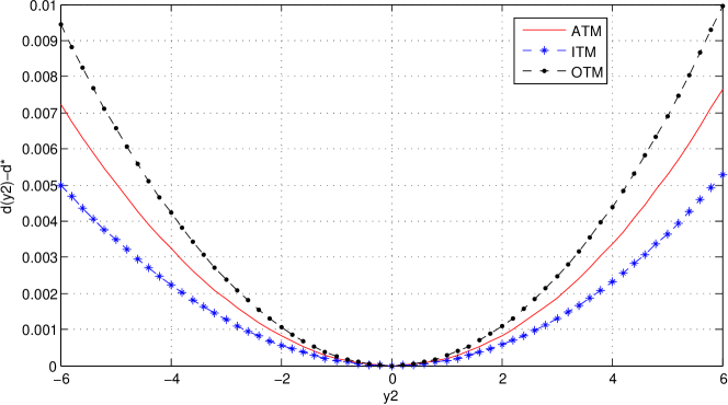
(a) Exact exercise boundary

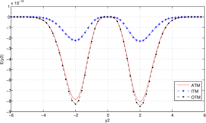
(b) Error density

Figure 2. (a) The exact exercise boundary of the 2 $\times$ 10 swaptions in Parameter Set 1. The strikes for ATM, ITM and OTM are 5.06%, 3.51% and 6.62%, respectively. Our method approximates this boundary as the horizontal axis $d(y_{2})=d^{*}$. Both the $x$ and $y$ axes are normalized by the standard deviation of the state variables. Although the distance between the exact boundary and the hyperplane grows quadratically from the tangent point, the probability of the normal distribution decays significantly faster. (b) The error density defined in Eq. (3.17) for the same swaptions and parameter sets. It is the probability-weighted swaption payoff integrated over the area between the exact boundary $\partial\Omega$ and the approximated hyperplane $\partial\tilde{\Omega}$ (shaded area in Fig. 1) in the direction of $y_{1}$. The error peaks at approximately two standard deviations and quickly decays because of the normally distributed probability density.

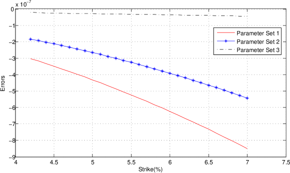
Figure 3. The implied volatility errors of the hyperplane approximation for varying strikes in daily basis point units. We use a 2 $\times$ 10 payer swaption against the three parameter sets. Although the error increases as the swaption becomes more out-of-the money, the approximation results remain good for very high strikes.

We further analyze the error using a particular example: a $2\times 10$ swaption on Parameter Set 1. First, we present the exact exercise boundary for this case in Fig. 2(a). The boundary lines for different strikes are slightly convex upward but are close to flat lines. In our method, by approximating the boundary with a flat line, we incorrectly exercise the swaption when the state falls into the area between the boundaries where the underlying swap has a negative value. Thus, we have a negative pricing error of $-2.8\times 10^{-5}$ for ATM. In Fig. 2(b), we provide the error density as defined in Eq. (3.17). Finally, we plot the DBP volatility error as a function of the strike in Fig. 3. For all three parameter sets, the error tends to increase for a higher strike. This increase is most likely because each term in Eq. (3.3) becomes more convex as the state becomes larger; this increases the deviation between the exercise boundary and the flat line.

References

- Andersen and Piterbarg [2010a] Leif B.G. Andersen and Vladimir V. Piterbarg. Interest Rate Modeling. Volume 2: Term Structure Models, chapter 10.2.5. Atlantic Financial Press, August 2010a. ISBN 0984422110.
- Andersen and Piterbarg [2010b] Leif B.G. Andersen and Vladimir V. Piterbarg. Interest Rate Modeling. Volume 2: Term Structure Models, chapter 12.1.3. Atlantic Financial Press, August 2010b. ISBN 0984422110.
- Andersen and Piterbarg [2010c] Leif B.G. Andersen and Vladimir V. Piterbarg. Interest Rate Modeling. Volume 2: Term Structure Models, chapter 13.1.5. Atlantic Financial Press, August 2010c. ISBN 0984422110.
- Bakshi and Madan [2000] Gurdip Bakshi and Dilip Madan. Spanning and derivative-security valuation. Journal of Financial Economics, 55(2):205–238, February 2000.
- Choi et al. [2009] Jaehyuk Choi, Kwangmoon Kim, and Minsuk Kwak. Numerical approximation of the implied volatility under arithmetic brownian motion. Applied Mathematical Finance, 16(3):261–268, 2009. doi: 10.1080/13504860802583436.
- Collin-Dufresne and Goldstein [2002] Pierre Collin-Dufresne and Robert S. Goldstein. Pricing swaptions within an affine framework. Journal of Derivatives, 10(1):9–26, 2002.
- Duffie et al. [2000] Darrell Duffie, Jun Pan, and Kenneth J Singleton. Transform analysis and asset pricing for affine jump-diffusions. Econometrica, 68(6):1343–1376, November 2000.
- Heath et al. [1992] David Heath, Robert A. Jarrow, and Andrew Morton. Bond pricing and the term structure of interest rates: A new methodology for contingent claims valuation. Econometrica, 60(1):77–105, 1992.
- Ho and Lee [1986] Thomas S Y Ho and Sang-bin Lee. Term structure movements and pricing interest rate contingent claims. Journal of Finance, 41(5):1011–29, December 1986.
- Hull and White [1990] John Hull and Alan White. Pricing interest-rate-derivative securities. Review of Financial Studies, 3(4):573–92, 1990.
- Munk [1999] Claus Munk. Stochastic duration and fast coupon bond option pricing in multi-factor models. Review of Derivatives Research, 3(2):157–181, 1999. ISSN 1380-6645.
- Schrager and Pelsser [2006] David F Schrager and Antoon A. J Pelsser. Pricing swaptions and coupon bond options in affine term structure models. Mathematical Finance, 16(4):673–694, October 2006. ISSN 1467-9965.
- Singleton and Umantsev [2002] Kenneth J Singleton and Len Umantsev. Pricing coupon-bond options and swaptions in affine term structure models. Mathematical Finance, 12(4):427–446, October 2002. ISSN 1467-9965.
- Vasicek [1977] Oldrich Vasicek. An equilibrium characterization of the term structure. Journal of Financial Economics, 5(2):177–188, November 1977.