Performance Analysis of C-V2I-based
Automotive Collision Avoidance

Abstract

One of the key applications envisioned for C-V2I (Cellular Vehicle-to-Infrastructure) networks pertains to safety on the road. Thanks to the exchange of Cooperative Awareness Messages (CAMs), vehicles and other road users (e.g., pedestrians) can advertise their position, heading and speed and sophisticated algorithms can detect potentially dangerous situations leading to a crash. In this paper, we focus on the safety application for automotive collision avoidance at intersections, and study the effectiveness of its deployment in a C-V2I-based infrastructure. In our study, we also account for the location of the server running the application as a factor in the system design. Our simulation-based results, derived in real-world scenarios, provide indication on the reliability of algorithms for car-to-car and car-to-pedestrian collision avoidance, both when a human driver is considered and when automated vehicles (with faster reaction times) populate the streets.

I Introduction

In recent years, the development of vehicular network applications has been attracting increasing interest from industries and researchers. A critical field of application of vehicular networks is represented by safety; indeed, in 2015 the number of people who lost their lives in road traffic is more than 1.2 million [1] and an increasing trend in road casualties was observed in 2016 [2]. A most significant and, at the same time, challenging safety application is collision detection. One of the basic requirements for vehicles running such an application is that they periodically send Cooperative Awareness Message (CAM) to a detector [3]. These messages are sent anonymously [4] toward the base station (BS) and contain information about position, speed, acceleration and direction of the sender. The collision detector combines all the CAMs received by the vehicles determining if any couple of vehicles is on a collision course. If so, the drivers involved are immediately alerted. The communication between vehicles and detectors happens through BSs that make communication possible even in non-line-of-sight (NLoS) conditions, e.g., due to buildings or other obstacles.

The application can be extended also to vulnerable road users such as pedestrians, whose smartphone can send CAMs to the detector. In this way, both drivers and pedestrians are timely made aware of possible life-threatening situations and can take proper action.

The purpose of this paper is to evaluate the performance of a system for vehicle-with-vehicle and vehicle-with-pedestrian collision detection when cellular vehicle-to-infrastructure (C-V2I) is adopted as a communication technology. In particular, we are mainly interested in the number of collisions that could be avoided and in the number of false positive alerts (i.e., alert messages referring to situations of low or no danger, that the system delivers to the users). Indeed, a low number of false positive alerts is essential in establishing user confidence in the reliability of alerts received through the system.

The remainder of this paper is organized as follows: Section II reviews the research related to the automotive collision avoidance application. Our reference scenario is introduced in Section III, while Section IV presents the design of the automotive collision avoidance system, along with the detection algorithm. The description of the methodology for our simulations and the output analysis technique are in Section V. Section VI contains the results obtained; the paper closes with our conclusions and future research directions in Section VII.

II Related Work

There are several works in the literature that are related to safety applications in the automotive domain (e.g., [5]). Many of these works, such as [6] and [7], propose collision avoidance and collision detection applications that do not leverage any mobile network infrastructure. In particular [6] focuses on collisions between vehicles and pedestrians in industrial plants. In this case, positioning is achieved using a combination of GPS, MEMS and smart sensors, while the type of wireless communication to the control center is not specified. In [7], White et al. propose a way to automatically detect a collision after it has occurred, using smartphone accelerometers to reduce the time gap between the actual collision and the first aid dispatch.

Our solution proposes a trajectory-based collision detection system based on a state-of-the art algorithm that we enhanced to match our needs. The same base-algorithm has been used, in different flavors, in [8] and [9]. [8] offers a top-down and specification driven design of an adaptive, peer-to-peer based collision warning system, while [9] proposes a V2V-like approach. However, those two works offer little simulation results. In particular, [8] only focuses on the collision avoidance algorithm, with little attention paid to implementation and network infrastructure. [9] provides some simulation results, but they tended to focus on the study of the algorithm parameters rather than applying the proposed solution to a realistic scenario.

An attempt to evaluate automotive forward collision warning and avoidance algorithm (CW/CA) has been done in [10], where K. Lee et al. evaluated five different CW/CA logics proposed by car makers. A very good survey of the strengths and weaknesses of LTE as an enabler of vehicular communication technology is [11], where Araniti et al. also extended some of the standardized safety messages used in this work.

III Reference Scenario

The reference topology we consider (depicted in Fig. 1) is an urban area composed of three roads, crossing at two intersections, a pedestrian lane and three pedestrian crossings. The intersections and crossings are unregulated, which makes collisions more likely. The entities moving in the topology are vehicles and pedestrians. Each of them is connected to the cellular infrastructure and uses the collision avoidance service, i.e., we assume a penetration rate equal to 1. Vehicles are equipped with on-board units for C-V2I communications, whereas pedestrians carry a smartphone with cellular connectivity. Both periodically send CAMs toward the collision avoidance application server.

In particular, we consider an LTE network with an eNodeB (eNB) located at the center of the topology. The server hosting the collision detector can be located at different points of the network infrastructure, i.e., at the eNodeB itself or at more remote network nodes. In order to study the difference in performance, we consider two server deployments: at the Metro node (very close to the eNB), in a multi-access edge computing (MEC) fashion, and in the Cloud (farther from the eNB). The choice of this urban topology allows us to have a simple but, at the same time, representative scenario, which closely mimics many real-world urban road layouts.

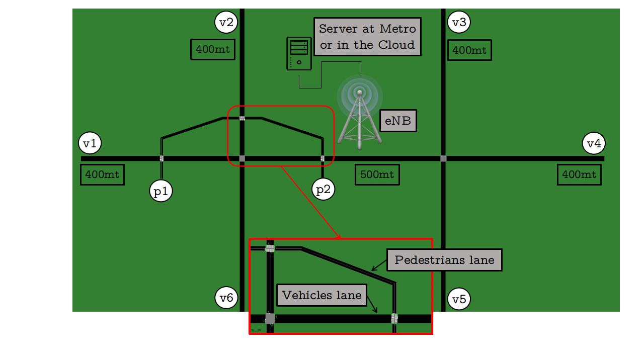
Figure 1: Screenshot of the simulated scenario in SUMO.

In order to assess the performance of the collision detection service in our scenario, we use the SimuLTE-Veins simulator [12], which leverages the mobility simulator SUMO [13].

III-A Populating the Scenario

We use a realistic mobility model and a realistic generation rate of both vehicles and pedestrians. Vehicles have a maximum speed of $13.89$ m/s (i.e., 50 km/h) and they follow a straight path, i.e., there are neither left nor right turns at junctions; pedestrians move with maximum speed of 2 m$/$s on the pedestrian lane, crossing the street at three different spots. Each generated vehicle is randomly assigned to one of the six entry points at the edge of the map (shown in Fig. 1 and marked as v1…v6), while each vulnerable user is assigned to one of either ends of the pedestrian lane (p1 or p2). Following [14], vehicle arrivals are modeled as a Poisson process with parameter $\lambda_{v}$; similarly, we model pedestrian arrivals with a different Poisson process with rate $\lambda_{p}$.

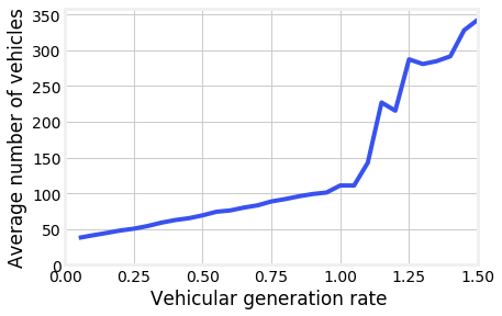
Figure 2: Evolution of the average number of vehicles for $\lambda_{p}=0.2$ and $\lambda_{v}$ varying from $0$ to $1.5$.

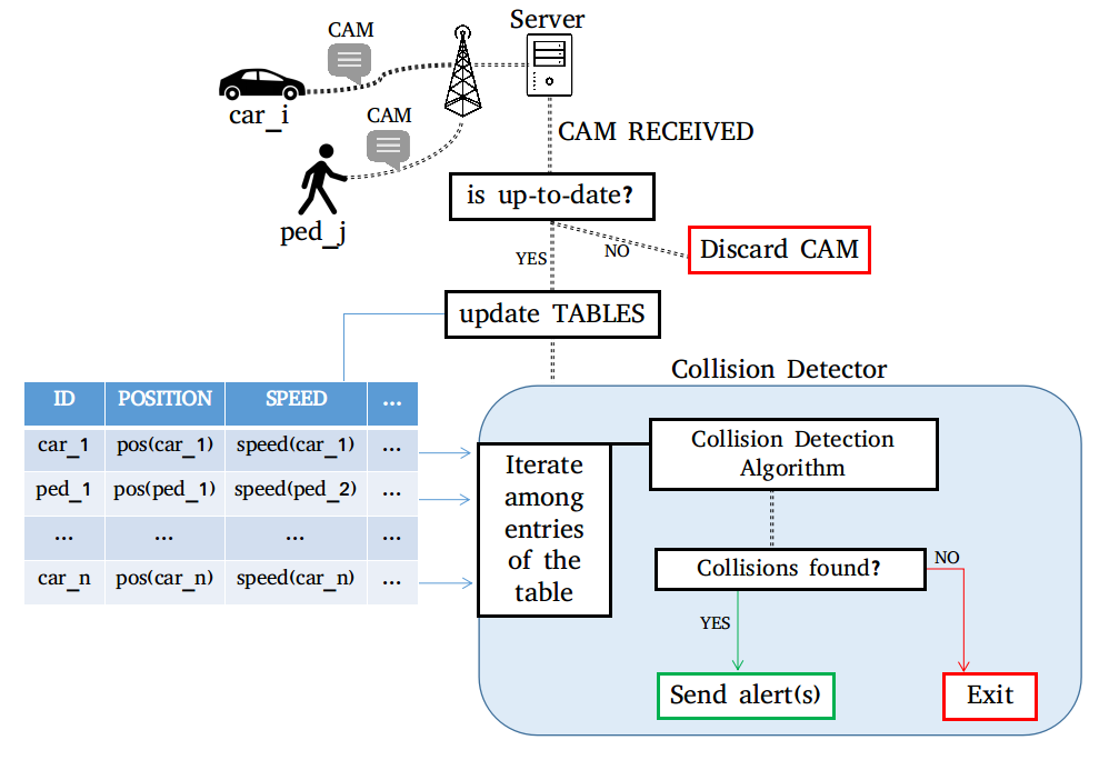
Figure 3: Collision avoidance system.

In order to have reliable results and a realistic mobility pattern, we apply the following methodology. We set both the vehicular generation rate $\lambda_{v}$ and the pedestrian generation rate $\lambda_{p}$ in such a way that the simulated scenario is stable; in other words, the number of vehicles or pedestrians should never grow so high as to yield the following situations:

1. too many cars start clogging the intersection;

2. the long queues of low-speed vehicles result into a negligible number of collisions, and so the effectiveness of the automotive collision avoidance application cannot be correctly evaluated.

The dependence of the number of vehicles and pedestrians from $\lambda_{v}$ and $\lambda_{p}$ is not linear because of the three crossings in which the two entities share the road occupancy. To properly select the arrival rate of both cars and pedestrians, we simulated the system when $\lambda_{v}$ varies from $0$ to $1.5$ whereas $\lambda_{p}$ takes one of five possible values: $0,0.05,0.10,0.15,0.20$. The results without pedestrians (i.e., $\lambda_{p}=0$) show that the value of $\lambda_{v}$ for which the average number of vehicles in the simulation grows linearly with the generation rate (i.e., it is in the stability region) is between $0$ and $1.2$. The introduction of pedestrians, however, has a significant impact: while with $\lambda_{p}=0$ the maximum $\lambda_{v}$ allowing stability is $1.2$, by increasing $\lambda_{p}$ to $0.2$, only values lower than $0.9$ ensure stability. Fig. 2 shows how the average number of vehicles evolves for different values of $\lambda_{v}$ with $\lambda_{p}$ fixed to $0.2$.

Consequently, we set $\lambda_{p}$ to $0.1$ and $\lambda_{v}$ to $0.7$. The value of $\lambda_{v}$ that we selected is consistent with real-world measurements from the city of Turin, Italy [15].

IV Design of the Collision Avoidance System

The collision detection system that we developed is shown in Fig. 3. Below, we first introduce the collision detection algorithm (Section IV-A), then we present the system design (Section IV-B). Finally, we show how to set the system parameters (Section IV-C).

IV-A The Collision Detection Algorithm

The core of the collision avoidance service is the detection algorithm. Although our algorithm accounts for the vehicle acceleration, Algorithm 1 presents a simplified version for the sake of clarity. Note that, being a generic trajectory-based algorithm, it can be applied to any kind of colliding entity (in our case both for vehicle-vehicle and vehicle-pedestrian collisions).

Algorithm 1 Collision detection pseudocode

1:$\vec{x_{0}},\vec{v},\mathcal{B}$

2:$\mathcal{C}\leftarrow\emptyset$

3:$\vec{x}(t)\leftarrow\vec{x_{0}}+\vec{v}t$

4:for all $b\in\mathcal{B}$ do

5:     $\vec{x^{b}}(t)\leftarrow\vec{x_{0}^{b}}+\vec{v^{b}}\cdot t$

6:     $\vec{d}(t)\leftarrow\vec{x}(t)-\vec{x^{b}}(t)$

7:     $D(t)\coloneqq|\vec{d}(t)|^{2}\leftarrow(\vec{v}-\vec{v^{b}})\cdot(\vec{v}-\vec{v^{b}})t^{2}+2(\vec{x_{0}}-\vec{x_{0}^{b}})\cdot\newline {\color[rgb]{1,1,1}iiiiiiiiiiiiii}\cdot(\vec{v}-\vec{v^{b}})t+(\vec{x_{0}}-\vec{x_{0}^{b}})\cdot(\vec{x_{0}}-\vec{x_{0}^{b}})$

8:     $t^{\star}\coloneqq t\colon\frac{\mathrm{d}}{\mathrm{d}t}D(t)=0\leftarrow\frac{-(\vec{x_{0}}-\vec{x_{0}^{b}})\cdot(\vec{v}-\vec{v^{b}})}{|\vec{v}-\vec{v^{b}}|^{2}}$

9:     if $t^{\star}<0\textbf{ or }t^{\star}>t2c_{t}$ then

10:         continue      

11:     $d^{\star}\leftarrow\sqrt{D(t^{\star})}$

12:     if $d^{\star}\leq s2c_{t}$ then

13:         $\mathcal{C}\leftarrow\mathcal{C}\cup\{b\}$      

14:return $\mathcal{C}$

The algorithm, which is based on [16], is run when, after receiving a CAM, the detector determines that the sender of the message is on a collision course with another node. The collision detection algorithm requires as input (Line 0):

• position and speed of the current vehicle, respectively identified by the two vectors $\vec{x_{0}}$ and $\vec{v}$; note that the speed vector also includes information on the heading;

• the latest CAM sent by each vehicle in the scenario stored in $\mathcal{B}$.

In Line 1, the set $\mathcal{C}$ of nodes with which the current entity could collide is initialized and, in Line 2, the future position of the current entity is evaluated for each future time instant. Then the algorithm computes the position of each node $b\in\mathcal{B}$ that recently sent a CAM (Line 4) and the distance $\vec{d}(t)$ between such a node and the current entity (Line 5). In Line 6, we compute the square of the distance $D(t)\coloneqq|\vec{d}(t)|^{2}$; we do this to simplify the subsequent computations. Since we are interested in the minimum value of $D(t)$, in Line 7 we compute $t^{\star}$, defined as the time instant at which the distance between the two entities is minimum . If $t^{\star}<0$, the two entities are getting farther apart, whereas, if $t^{\star}$ is greater than a threshold $t2c_{t}$ (where $t2c$ stands for time to collision), the minimum distance will not be reached within $t2c_{t}$ from the current time. In both cases, no action is required (Line 8). If $t^{\star}$ is between 0 and $t2c_{t}$, in Line 11 the minimum distance $d^{\star}$ at which the two entities will be at time $t^{\star}$ is computed. The algorithm compares $d^{\star}$ against a minimum threshold $s2c_{t}$ (space to collision): if $d^{\star}$ is lower, then vehicle $b$ is added to set  $\mathcal{C}$, otherwise the algorithm skips to the next iteration of the cycle.

Once all of the CAMs in set $\mathcal{B}$ have been processed, the algorithm returns the set $\mathcal{C}$ of entities with which the current one is on a collision course. If the set $\mathcal{C}$ is empty, no action is taken, else an alert message is sent to the current entity as well as to all entities in set $\mathcal{C}$. We will discuss the setting of the thresholds $t2c_{t}$ and $s2c_{t}$ in Section IV-C.

IV-B System Description

Looking at Fig. 3, we now specify how the other system blocks work.

The frequency at which CAMs are sent by each entity is 10 Hz, which is the maximum frequency allowed by the ETSI standard [17]. This high value allows the whole system to work with updated information. Indeed, considering a lower frequency, e.g., 1 Hz, and a car moving at 13.89 m$/$s (i.e., 50 km$/$h), the error at the server (ignoring the transmission delays) would be in the worst case of 13.89 m. Clearly, such a high error is not acceptable when dealing with a safety application.

The detector placed at the server is able to distinguish between CAMs sent by pedestrians and CAM sent by vehicles. This gives us a double advantage. First, when the server receives a CAM from a vehicle, it looks for possible collisions with both cars and pedestrians, while on the contrary, with a message sent from a pedestrian, the algorithm skips the analysis for pedestrian-with-pedestrian collisions. The second advantage involves the possibility to set different parameters for the collision detection algorithm (i.e., $s2c_{t}$ and $t2c_{t}$), according to the type of entity which sent the CAM. This allows a better performance of the algorithm, in terms of false positives and false negatives.

Every time the detector receives a message, it checks if the message is up-to-date: if so, the server stores the information of the CAM; otherwise, the CAM is discarded. We set 0.8 s as the threshold beyond which a CAM is considered as stale and discarded. In the case of a fresh CAM, the algorithm checks if its sender is at risk of collision. To improve the system efficiency, we also introduce a range of action: only the entities within such a range will be checked by the algorithm as potential colliders. The radius varies according to the vehicle speed as follows:

$$\mbox{Radius}=\max\{\mbox{Speed}\cdot t2c_{t},s2c_{t}\}$$

When the server detects a pair of entities on a course of collision, they are warned by an alert message. In order to avoid an excessive number of duplicated alerts, the collision detector does not generate the same alert message more then one every second.

Thresholds and values used by the collision detector are summarized in Table I and discussed in the next section.

TABLE I: Collision detection parameters for vehicles and pedestrians.

Parameter	Value
	Vehicle	Pedestrian
$t2c_{t}$	10 s	5 s
$s2c_{t}$	5 m	2 m
Max CAM Age	0.8 s	0.8 s
CAM frequency	10 Hz	10 Hz
Alert max frequency	1 Hz	1 Hz

IV-C Sensitivity Study on Collision Thresholds

Here we investigate the two parameters that mainly affect the performance of the collision detection system: $t2c_{t}$ and $s2c_{t}$. Before delving into this study, we better detail their meaning below:

• $t2c_{t}$ is the time to collision threshold. It introduces an upper bound on the time to collision metric, i.e., the time gap needed for two entities to reach their mutual minimum distance. The higher this threshold, the more likely it is that a pair of entities are considered at risk of collision.

• $s2c_{t}$: it is the space to collision threshold. It is the upper bound to the distance at which two entities are at the time to collision, to consider them at collision risk. Obviously, the higher the threshold, the more likely it is that a pair of entities is considered in collision course.

Setting those two parameters has a big impact both on system accuracy and on system efficiency: relaxing them means to let the algorithm trigger too many alerts, even when candidates are not going to get that close. Of course, in this case all the collisions are correctly detected, but a large percentage of alerts refer to low-danger situations. On the other hand, being too strict leads to the opposite situation in which the number of unnecessary alerts is drastically reduced, but a percentage of the collisions goes undetected or detected too late. All the above are potentially dangerous for the driver. In particular, for false positives it should be taken into account that an excessive number of warnings may desensitize the driver, causing future alerts to be ignored [8].

For these reasons, we undertook a study on the number of undetected or late-detected collisions as well as on false positives, as functions of $s2c_{t}$ and $t2c_{t}$ (Fig. 4).

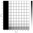
(a) Vehicle-with-vehicle: percentage of undetected or late-detected collisions

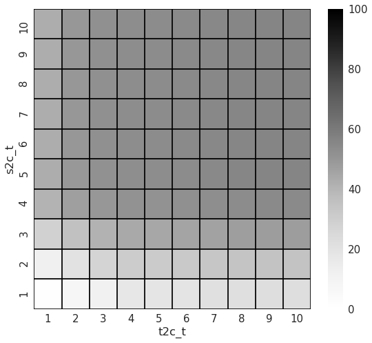
(b) Vehicle-with-vehicle: percentage of false positives

(c) Vehicle-with-pedestrian: percentage of undetected or late-detected collisions

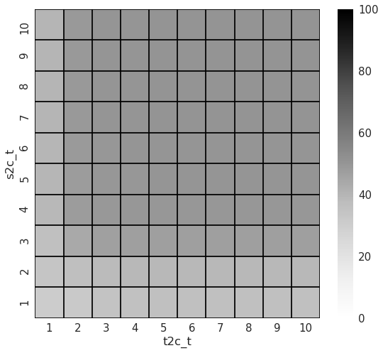
(d) Vehicle-with-pedestrian: percentage of false positives

Figure 4: Thresholds analysis for vehicles traveling at 50 km/h.

Looking at the heatmap in Fig. 4(a), it is clear that for values of $t2c_{t}$ equal or lower than 3 s, in a scenario where vehicles travel at or around 50 km/h, the system is completely unreliable. Indeed, considering the delays introduced by different factors (e.g., processing time, human reaction, braking time), sending the alert not earlier than 3 s before the expected impact, does not allow the driver to stop the vehicle and avoid the accident. Thus, the $t2c_{t}$ value needs to be at least 4 s. Looking at $s2c_{t}$ and considering $t2c_{t}$ equal to 4 s, any value greater than 3 m ensures the system to work efficiently, detecting in time the collisions occurred.

As mentioned before, the drawback of having high values of the threshold is the number of false positives. Fig. 4(b) shows that few false positives can be obtained only with very low thresholds (both $t2c_{t}$ and $s2c_{t}$ equal or lower than $2$), but this is completely unacceptable given the high percentage of collisions not detected or detected too late with such values. Thus, an interesting observation is that a high number of false positives is the price to pay in order to realize a reliable collision detection system.

Looking at the case of vehicle-with-pedestrian alerts, we observe a similar behavior. Fig. 4(c) shows that, even if the trend is the same, a better performance is achieved by using smaller values for the $t2c_{t}$ and $s2c_{t}$ thresholds. This happens because, in the case of an alert, a pedestrian can stop almost instantaneously due to her low speed. The above dynamic causes the total number of false positives to be in general higher than in the vehicle-with-vehicle case (Fig. 4(d)).

V Simulation Methodology

In this section, we first describe the approach we adopted to process the simulation logs in order to derive the main metrics of interest. We then detail how we discern whether alerts are received on time by the involved entities so that the collision can be avoided.

V-A Processing the Simulation Logs

We start by collecting the following information:

1. the dynamics of vehicles and pedestrians (e.g., their position, speed and heading), using the SUMO Floating Car Data output;

2. the vehicle-with-vehicle and vehicle-with-pedestrian collisions that occurred, through the SUMO error-log file;

3. all the alerts sent by the collision avoidance application, using the SimuLTE-Veins simulator.

Then, through post-processing, we analyze, for each collision, when it occurred and if the corresponding alert message was generated. Furthermore, if the alert was correctly transmitted, we also look at when it was received and processed by the involved entities. In this way, we can determine if the vehicle had sufficient time to brake before the impact.

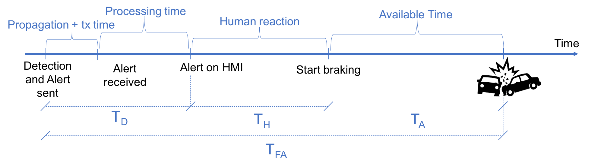
Figure 5: Timeline of the communication between the detection server and the human driver.

V-B Reaction to Alerts

Whether a collision is detected in time or too late is determined in the post-processing phase, by considering the alert messages that have been received. A collision is considered as “detected too late” if:

$$T_{A}<T_{B}$$

where $T_{A}$ represents the time available to the driver to avert the collision, i.e., the interval between when the driver initiates evasive actions and the actual collision. $T_{B}$, instead, is the time needed by the entity to stop, given its current speed and maximum deceleration. $T_{A}$ is computed as follows:

$$T_{A}=T_{FA}-T_{D}-T_{H}\,,$$ (1)

where the three elements in the above expression are:

• $T_{D}$: the time gap between the moment at which a collision is detected by the server and the moment at which the alert reaches the driver through the vehicle HMI. It includes the transmission time and the processing time. The transmission time includes the time to transfer data from the application server to the eNB, and then to the entities involved in the collision. The processing time is the time needed at the receiving node to process an alert message from the time instant at which the first bit is received to the time instant at which the driver is notified about the received information. The processing time is set to 400 ms [18];

• $T_{H}$: the time needed by a human driver to take action following the prompt of an alert. It is fixed to 1 second, as suggested by several studies [19] [20] that take in account different variables such as age, travel length, environment, etc. Note that this parameter is set to zero in the case of automated vehicles;

• $T_{FA}$: the time interval between the generation of the first alert related to a possible collision and when the actual collision occurs.

Fig. 5 provides a visual representation of the timeline of the communication between the collision detector and the human driver, highlighting the time intervals discussed above.

VI Performance Results

Below, we describe the simulation settings we used (Subsection VI-A), and we show our results in terms of collision detection accuracy and alert reliability (Subsection VI-B).

VI-A Simulation Settings

We run two sets of ten 300s-long simulations, one with the server at the Metro node and the other with the server placed in the Cloud. As exemplary values reflecting real-world mobile operators topologies, 5 ms and 20 ms have been chosen for the Metro-eNB and cloud-eNB latencies. In the post-processing phase, each of the two simulation sets is analyzed considering either the human driver or the automated vehicle case. Intuitive, a better performance can be expected in the automated vehicle scenario, as $T_{H}=0$.

VI-B Simulation Results

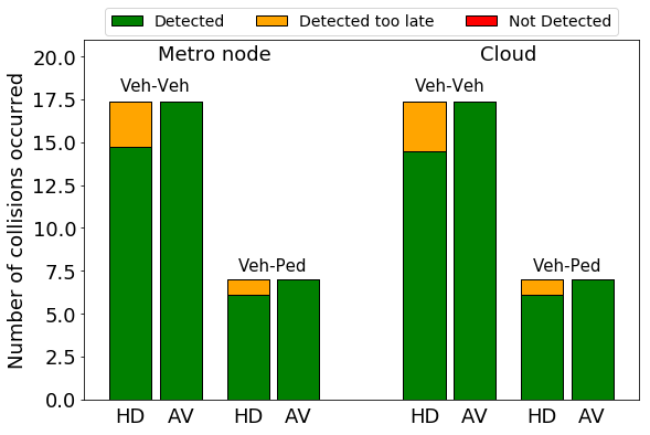
Figure 6: Vehicle-with-vehicle (Veh-Veh) and vehicle-with-pedestrian (Veh-Ped) collisions detected, detected too late and not detected, for the Human Driver (HD) case and the Autonomous Vehicle (AV) case, and for different server placements.

Fig. 6 shows the effectiveness of our collision avoidance system in terms of number of accidents that can be prevented. The four bars show the number of vehicle-with-vehicle detected, late-detected and undetected collisions among those reported by the SUMO simulator. A collision is reported in SUMO each time the polygon describing an entity overlaps with the polygon describing another entity. The two leftmost bars refer to the case in which the server is placed at the Metro node, both in the human driver case and in the automated vehicle case, while the other two refer to the scenario where the server is in the Cloud.

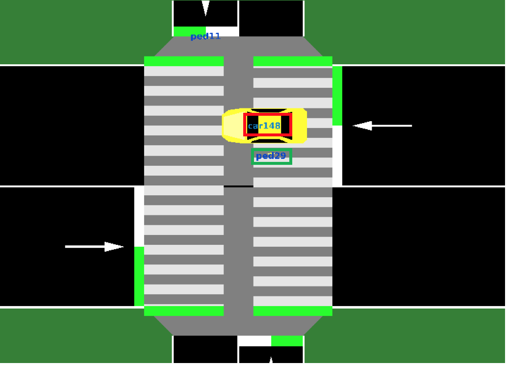
Figure 7: Screenshot from SUMO representing a situation that leads to a false negative.

The first important result that we highlight is the effectiveness of our algorithm: regardless of the location of the server, it reaches $100\%$ in case of automated vehicle, and over $80\%$ in case human driver. A second relevant result, is the absence of “Not detected” collisions in the four case studies. More in general, the histograms referring to the Metro node are quite similar to the ones referring to the Cloud, with the exception of few “Detected too late” cases: the latter show a little increase when the server is placed in the Cloud. The reasons for this limited increase are twofold. First, when a collision is correctly detected, the time between the generation of the first alert and the actual collision ($T_{FA}$) is around 10 seconds (which is the threshold $t2c_{t}$). Thus, relatively speaking, the delay introduced by moving the collision detector from the Metro node to the Cloud can be considered as negligible. Second, even if the $t2c_{t}$ value were reduced, the increased transmission time would not have an impact. Indeed, looking at the expression of $T_{A}$ in (1), the difference of 15 ms due to the location of the server, is very small compared to the processing time (400 ms) or, in case of human driver, to $T_{H}$ (1 s).

Next, we focus on the collisions between pedestrians and vehicles. The generation rate of pedestrians is relatively low (on average 1 pedestrian every 10 s), so the number of collisions observed is lower than in the previous case. We notice a decrease in the effectiveness of our collision detector, with about 6.5% of collisions going undetected. Furthermore, false negatives now affect all the case studies, regardless of the type of driver and the location of the server. Since the “undetected” collisions are very few, we scrutinized each of them. It turned out that all false negatives are due to the mobility model used in SUMO for pedestrians at zebra crossings and for the approaching vehicles. Let us consider a vehicle and a pedestrian approaching a free zebra crossing. Since no pedestrian occupies the crosswalk, the vehicle proceeds at maximum speed. Once the pedestrian enters the zebra crossing, the car, which now sees the obstacle, starts to decelerate. If it is impossible to stop in time, the “best” thing to do would be not to stop. However, according to the SUMO mobility model, the vehicle always tries to stop when approaching an occupied junction, thus the vehicle continues to decelerate. Our algorithm, which is aware of the speed, distance and acceleration of the car, predicts that the vehicle will never hit the pedestrian and, also, that when it stops completely, the pedestrian will be behind the car, thus no alerts are sent. However, as shown in Fig. 7, the vehicle stops in the middle of the crosswalk and the pedestrian, completing the crosswalk, rather than dodging it, physically walks over it. This is reported as a collision in the SUMO logs. By discounting this issue, the system performance becomes comparable to that of vehicular collision case, as depicted in Fig. 6. Looking at the histogram, moving the server to a farther location only minimally affects the “Detected too late” cases. This is because, whenever a possible collision is correctly detected, the pedestrian will have about 5 s (which is the $t2c_{t}$ threshold for the pedestrian case) to act, which is more than enough since pedestrians can stop almost instantaneously.

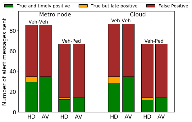
Figure 8: False positive statistics for vehicle-with-vehicle (Veh-Veh) and vehicle-with-pedestrian (Veh-Ped) collisions for the Human Driver (HD) case and the Autonomous Vehicle (AV) case, and for different server placements.

Another issue to investigate is the study of the quality of alerts that are actually received by the vehicles, in order to find the fraction of false positives, i.e., the alert messages referring to situations of low or no danger. False positives are not as critical as undetected collisions but they may be a cause of distraction for human drivers. The list of the metrics studied in this section follows:

• total alert sent: total number of alerts sent by the server to vehicles to warn them about detected collisions.

• true positives: alerts that have been sent and refer to collisions that actually occurred. They include:

  • true and timely positives: alerts for which the driver had enough time to brake before the collision happened;

  • true but late positives: alerts for which the driver did not have enough time to brake before the collision happened.

• false positives: alerts that have been sent and refer to collisions that would not take place.

Fig. 8 shows the results of this analysis. The false positive percentage is high, greater than 60%. As was explained in Section IV-C, the value of false positives may decrease by decreasing the values of the thresholds $t2c_{t}$ and $s2c_{t}$.

This high value of false positive alerts brings us to analyze their relevance. We therefore look at the minimum distance reached by the pairs of vehicles receiving false positives alerts to determine if, also in absence of collision, a dangerous situation has arisen. By parsing the Floating Car Data SUMO output, we checked, for each pair of vehicles warned by a false positive alert, the minimum distance that the two vehicles reached over the time. The Cumulative Density Function (CDF) of this quantity is shown in Fig. 9. This plot tells us that:

• 60% of the false positive alerts are sent to vehicles that got less than 2.3 m apart;

• there are no vehicles warned by a false positive alert whose minimum distance is more than 5 m.

This highlights that the false positive alerts are transmitted in situations that are indeed dangerous – a factor that is particularly important when inaccuracies of the positioning system are taken into account.

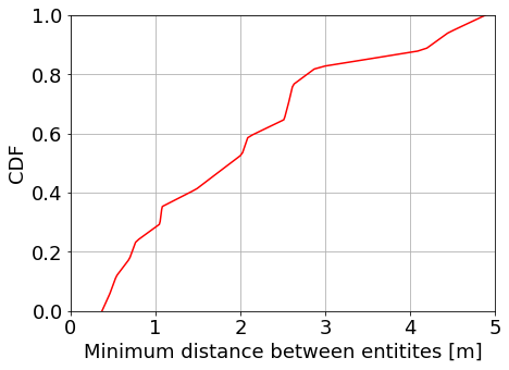
Figure 9: CDF of the distance between cars in a false positive situation.

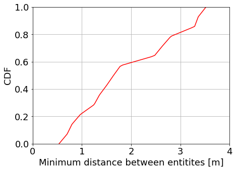
Figure 10: CDF of the vehicle-to-pedestrian distance in a false positive situation.

As far as the vehicle-with-pedestrian false positive alerts are concerned, the results are shown in Fig. 8. The histograms portray a situation that is more critical than in vehicle-to-vehicle collisions. Indeed, the false positive rate is around 80%. This behavior is due to the characteristics of the pedestrian mobility with respect to cars: zebra crossings are occupied for a longer time by pedestrians, in particular, since pedestrians move at a maximum speed of 2 m$/$s and the two lanes are each 6 m wide, a pedestrian will occupy the crossing for about 6 seconds. During this time, it is likely that other cars will approach the crossing and, if they stop or pass close to the pedestrian, the collision detector will trigger the generation of an alert, even if no collision actually occurs. In this case too, it is important to look at the CDF of the vehicle-to-pedestrian distance (Fig. 10), which shows that 50% of the false positives are sent for situations in which the car and the pedestrian were 2 m apart from each other.

As a final remark, although the percentage of false positives is quite high, a C-V2I-based system can ensure high reliability in collision detection, and even false positives refer to actually dangerous situations. Furthermore, large margins of improvement are possible if additional information coming from on-board sensors (cameras, radars, lidars…) is merged with that available through the C-V2I interface, and advanced data fusion algorithms are used so as to provide the driver with a comprehensive, yet accurate, warning system.

VII Discussion and Conclusions

In this paper, we have proposed an efficient C-V2I-based system for automotive collision avoidance, and tested it under different scenarios. By exploiting the transmission of CAMs toward the collision detection server, the latter determines whether any pair of vehicles, or vehicle and pedestrian, are set on a collision course, and, if so, it issues an alert message. We deployed the server in two different points of the network, namely, in the Metro node and in the Cloud, and we considered both human drivers and automated vehicles.

Our results show that in every case study we analyzed, the percentage of detected collisions is $100\%$. However, considering a human driver, a percentage of those collisions (on average $14\%$) is detected too late. Considering automated vehicle instead, due to the absence of the human reaction time, no late-detected collisions are observed. Additionally, in this case, the different location of the server does not have a noticeable impact on the system performance, given the values for human reaction time and on-board processing time.

As far as the analysis of alert messages sent by the server is concerned, we see that a high percentage thereof are false positives. At a closer inspection, we found that, even if the number of false positive alerts is very high, they are sent in situations that are actually dangerous. This fact is particularly important if inaccuracies of the positioning system are taken into account.

Two main directions for future research can be envisioned: (i) investigating the gain that cellular vehicle-to-vehicle (C-V2V) communications can bring; (ii) assessing the benefits that may come from data fusion performed on CAMs and sensory data such as those collected via cameras, radars and lidars.

References

- [1] World Health Organization. (2016) Global Status Report on Road Safety 2015. http://www.who.int/violence_injury_prevention/road_safety_status/2015/en/.
- [2] Road Safety Annual Report. http://www.sipotra.it/wp-content/uploads/2017/10/Road-Safety-Annual-Report-2017.pdf.
- [3] C. Sommer, S. Joerer, M. Segata, O. K. Tonguz, R. L. Cigno, and F. Dressler, “How shadowing hurts vehicular communications and how dynamic beaconing can help,” IEEE Transactions on Mobile Computing, 2015.
- [4] F. Malandrino, C. Borgiattino, C. Casetti, C. F. Chiasserini, M. Fiore, and R. Sadao, “Verification and Inference of Positions in Vehicular Networks through Anonymous Beaconing,” IEEE Transactions on Mobile Computing, 2014.
- [5] L. Gallo and J. Haerri, “Unsupervised long-term evolution device-to-device: A case study for safety-critical v2x communications,” IEEE Vehicular Technology Magazine, vol. 12, no. 2, pp. 69–77, June 2017.
- [6] Z. Riaz, D. Edwards, and A. Thorpe, “SightSafety: A hybrid information and communication technology system for reducing vehicle/pedestrian collisions,” Elsevier Automation in construction, 2006.
- [7] J. White, C. Thompson, H. Turner, B. Dougherty, and D. C. Schmidt, “Wreckwatch: Automatic traffic accident detection and notification with smartphones,” Springer Mobile Networks and Applications.
- [8] R. Miller and Q. Huang, “An adaptive peer-to-peer collision warning system,” IEEE Vehicular Technology Conference, 2002.
- [9] Y. Wang, E. Wenjuan, D. Tian, G. Lu, G. Yu, and Y. Wang, “Vehicle collision warning system and collision detection algorithm based on vehicle infrastructure integration,” Advanced Forum on Transportation of China, 2011.
- [10] K. Lee and H. Peng, “Evaluation of automotive forward collision warning and collision avoidance algorithms,” Vehicles System Dynamics, 2005.
- [11] G. Araniti, C. Campolo, M. Condoluci, A. Iera, and A. Molinaro, “LTE for vehicular Networking: A Survey,” IEEE Communications Magazine, 2013.
- [12] SimuLTE and Veins. http://simulte.com/add_veins.html.
- [13] SUMO – Simulation of Urban MObility. http://www.dlr.de/ts/en/desktopdefault.aspx/tabid-9883/16931_read-41000/.
- [14] Y. Li, D. Jin, Z. Wang, P. Hui, L. Zeng, and S. Chen, “A markov jump process model for urban vehicular mobility: Modeling and applications,” IEEE Transactions on Mobile Computing, 2014.
- [15] 5T Open data repository. http://www.5t.torino.it/open-data/.
- [16] F. Gong, B. Gao, and Q. Niu, “An Algorithm for Rapidly Computing the Minimum Distance between Two Objects Collision Detection,” in 2008 Congress on Image and Signal Processing, 2008.
- [17] ETSI EN 302 637-2 V1.3.1 (2014-09), Intelligent Transport System (ITS);. Vehicular Communications; Basic Set of Applications. http://www.etsi.org/deliver/etsi_en/302600_302699/30263702/01.03.01_30/en_30263702v010301v.pdf.
- [18] H. G.-P. G.-C. Project. (2017) 5G-CAR Scenarios, Use Cases, Requirements and KPIs. https://5gcar.eu/wp-content/uploads/2017/05/5GCAR_D2.1_v1.0.pdf.
- [19] Driver’s reaction time. http://copradar.com/redlight/factors/index.html.
- [20] H. Summala, “Brake reaction times and driver behavior analysis,” Transportation Human Factors, 2000.