Curious convergence properties

of lattice Boltzmann schemes

for diffusion with acoustic scaling

Bruce M. Boghosian^a, François Dubois^bc, Benjamin Graille^b,

Pierre Lallemand^d and Mohamed-Mahdi Tekitek^e

^a Dpt. of Mathematics, Tufts University, Bromfield-Pearson Hall, Medford, MA 02155, U.S.A.

^b Dpt. of Mathematics, University Paris-Sud, Bât. 425, F-91405 Orsay, France.

^c Conservatoire National des Arts et Métiers, LMSSC laboratory, F-75003 Paris, France.

^d Beijing Computational Science Research Center, Haidian District, Beijing 100094, China.

^e Dpt. Mathematics, Faculty of Sciences of Tunis, University Tunis El Manar, Tunis, Tunisia.

24 March 2017

Keywords: artificial compressibility method, Taylor expansion method.

PACS numbers: 02.70.Ns, 05.20.Dd, 47.10.+g

Abstract

We consider the D1Q3 lattice Boltzmann scheme with an acoustic scale for the simulation of diffusive processes. When the mesh is refined while holding the diffusivity constant, we first obtain asymptotic convergence. When the mesh size tends to zero, however, this convergence breaks down in a curious fashion, and we observe qualitative discrepancies from analytical solutions of the heat equation. In this work, a new asymptotic analysis is derived to explain this phenomenon using the Taylor expansion method, and a partial differential equation of acoustic type is obtained in the asymptotic limit. We show that the error between the D1Q3 numerical solution and a finite-difference approximation of this acoustic-type partial differential equation tends to zero in the asymptotic limit. In addition, a wave vector analysis of this asymptotic regime demonstrates that the dispersion equation has nontrivial complex eigenvalues, a sign of underlying propagation phenomena, and a portent of the unusual convergence properties mentioned above.

1)  Introduction

Lattice Boltzmann models are simplifications of the continuum Boltzmann equation obtained by discretizing in both physical space and velocity space. The discrete velocities $v_{i}$ retained typically correspond to lattice vectors of the discrete spatial lattice. That is, each lattice vertex $x$ is linked to a finite number of neighboring vertices by lattice vectors $v_{i}\,\Delta t$. A particle distribution $\,f\,$ is therefore parametrized by its components in each of the discrete velocities, the vertex $x$ of the spatial lattice, and the discrete time $t$. A time step of a classical lattice Boltzmann scheme [11] then contains two steps:

(i) a relaxation step where distribution $f$ at each vertex $x$ is locally modified into a new distribution $f^{*}$, and

(ii) an advection step based on the method of characteristics as an exact time-integration operator. We employ the multiple-relaxation-time approach introduced by d’Humières [10], wherein the local mapping $\,f\longmapsto f^{*}\,$ is described by a nonlinear diagonal operator in a space of moments, as detailed in Section 2.

In [5], we have studied the asymptotic expansion of various lattice Boltzmann schemes with multiple-relaxation times for different applications. We used the so-called acoustic scaling, in which the ratio $\,\lambda\equiv\Delta x/\Delta t\,$ is kept fixed. In this manner, we demonstrated the possibility of approximating diffusion processes described by the heat equation.

In his very complete work, Dellacherie [3] has described unexpected results in simulations for advection-diffusion processes. In this contribution, we endeavor to explain those results by studying the convergence of the D1Q3 lattice Boltzmann scheme when we try to approximate a pure diffusion process.

We begin this paper by recalling some fundamental algorithmic aspects of the D1Q3 lattice Boltzmann scheme in Section 2. Then, in Section 3 we describe a first illustrative numerical experiment. In Section 4 we present a new convergence analysis, followed by another numerical experiment in Section 5, in which the D1Q3 lattice Boltzmann scheme is studied far from the usual values of its parameters. Finally, a wave vector analysis is proposed in Section 6.

2)  Diffusive D1Q3 lattice Boltzmann scheme

In this work, we consider the so-called D1Q3 lattice Boltzmann scheme in one spatial dimension. The spatial step $\,\Delta x>0\,$ is given, and each node $\,x\,$ is an integer multiple of this spatial step : $\,x\in\mathbb{Z}\,\Delta x$. The time step $\,\Delta t>0\,$ is likewise given, and each discrete time $\,t\,$ is an integer multiple of $\,\Delta t$. We adopt so-called acoustic scaling (see e. g., [12]), so the numerical velocity associated with the mesh,

(1) $$\lambda\equiv{{\Delta x}\over{\Delta t}},\vspace*{-7pt}$$

is a constant independent of the spatial step $\,\Delta x$. A particle distribution

$$f\,\equiv\,\big{(}f_{+}(x,\,t)\,,\,f_{0}(x,\,t)\,,\,f_{-}(x,\,t)\big{)}\vspace*{-6pt}$$

is given at the initial step $\,t=0$. Its value at subsequent times is determined by the multiple-relaxation-time version [10] of the lattice Boltzmann equation.

$\bullet$  Moments are introduced at each step of space and time according to the relations

(2) $$\rho=f_{+}+f_{0}+f_{-}\,,\quad J=\lambda\,(f_{+}-f_{-})\,,\quad e=\lambda^{2}\,(f_{+}-2\,f_{0}+f_{-})\,.\vspace*{-7pt}$$

These may be thought of as the densities of mass, momentum, and an energy-like quantity, respectively. Eq. (2) can be recast in matrix form as follows:

$$m\,\equiv\,\begin{pmatrix}\rho\cr J\cr e\end{pmatrix}\,=\,M\,f\,\equiv\,M\,\begin{pmatrix}f_{+}\cr f_{0}\cr f_{-}\end{pmatrix}\,,\vspace*{-6pt}$$

where $\,M\,$ is the invertible matrix,

(3) $$M\,=\,\begin{pmatrix}1&1&1\cr\lambda&0&-\lambda\cr\lambda^{2}&-2\,\lambda^{2}&\lambda^{2}\end{pmatrix}\,.\vspace*{-7pt}$$

$\bullet$  The equilibrium values of the moments are defined by the relations:

(4) $$\rho^{\rm eq}=\rho\,,\quad J^{\rm eq}=0\,,\quad e^{\rm eq}=\alpha\,{{\lambda^{2}}\over{2}}\,\rho\vspace*{-7pt}$$

where $\,\alpha\,$ a non-dimensional constant. Then the relaxation step transforms the pre-collision moments $\,m\,$ into new post-collision moments $\,m^{*}$ as follows:

(5) $$\rho^{*}=\rho\,,\quad J^{*}=J+s_{J}\,(J^{\rm eq}-J)\,,\quad e^{*}=e+s_{e}\,(e^{\rm eq}-e)\,,\vspace*{-7pt}$$

where $s_{J}$ and $s_{e}$ are relaxation parameters. There is no analogous parameter for $\rho$ because the collisions are constrained to conserve mass. In our numerical experiments, we have chosen $\,s_{e}=1.5$, and below we shall explain in some detail how we tuned the relaxation parameter $\,s_{J}\,$ for the momentum $\,J$.

$\bullet$  The time iteration of the scheme is defined in terms of the particle distribution. We first transform the post-collision moments $\,m^{*}\,$ into a post-collision particle distribution:

$$f^{*}\,=\,M^{-1}\,m^{*}\,.\vspace*{-6pt}$$

Second, we iterate the algorithm forward in time. The particle distribution is conserved along the characteristic directions of velocities $\,v_{+}=\lambda$, $\,v_{0}=0\,$ and $\,v_{-}=-\lambda\,$ respectively:

(6) $$\left\{\begin{array}[]{l}\displaystyle f_{+}(x,\,t+\Delta t)\,=\,f_{+}^{*}(x-\Delta x,\,t)\cr f_{0}(x,\,t+\Delta t)\,\,=\,f_{0}^{*}(x,\,t)\cr f_{-}(x,\,t+\Delta t)\,=\,f_{-}^{*}(x+\Delta x,\,t)\,.\end{array}\right.\vspace*{-7pt}$$

$\bullet$  In [5], we have analyzed several lattice Boltzmann models with the Taylor expansion method, including the present one defined by Eqs. (2,3,4,5,6). The hypothesis used was that the numerical velocity $\,\lambda\,$ defined in Eq. (1), and the relaxation coefficients $\,s_{J}\,$ and $\,s_{e}\,$ remain constant as the spatial step $\,\Delta x\,$ tends to zero. Then the conserved variable $\,\rho\,$ satisfies (at least formally!) a diffusion partial differential equation:

(7) $${{\partial\rho}\over{\partial t}}\,-\,\mu\,\,{{\partial^{2}\rho}\over{\partial x^{2}}}\,=\,{\rm O}(\Delta x^{2})\,,\vspace*{-7pt}$$

where the diffusion coefficient $\mu\,$ is given by the relation

(8) $$\mu\,\equiv\,{{4+\alpha}\over{6}}\,\sigma\,\lambda\,\Delta x\,,\quad\sigma\,\equiv\,\Big{(}{{1}\over{s_{J}}}-{{1}\over{2}}\Big{)}\,.\vspace*{-7pt}$$

The coefficient $\,\sigma\,$ is known as the “Hénon parameter” in reference to the pioneering work of Hénon [9]. This lattice Boltzmann scheme is demonstrably stable under the condition:

$$-4\,<\,\alpha\,<\,2\,.\vspace*{-6pt}$$

3)  A first numerical experiment

In this section, we consider an elementary analytic test case, namely the diffusion of a sine wave. We suppose that the initial condition for Eq. (7) satisfies

(9) $$\rho_{0}(x)=\sin(\pi\ x)\,,\quad-1\leq x\leq 1\,.\vspace*{-7pt}$$

The other moments $\,J\,$ and $\,e\,$ are taken at equilibrium at $\,t=0$. With periodic boundary conditions, the exact solution of Eqs. (7,9) is

$$\rho(x,\,t)=\sin(\pi\,x)\,\exp(-\mu\,\pi^{2}\,t)\,.\vspace*{-6pt}$$

We performed several numerical computations with the following choice of parameters: $\,\lambda=1$, $\,\alpha=1\,$ and $\,\mu=0.01$. The spatial step varied from $\,\Delta x={1\over 4}\,$ up to $\,\Delta x={1\over 32}$. The results for a final time $\,T=5\,$ are presented in Figs. 1 through 3.

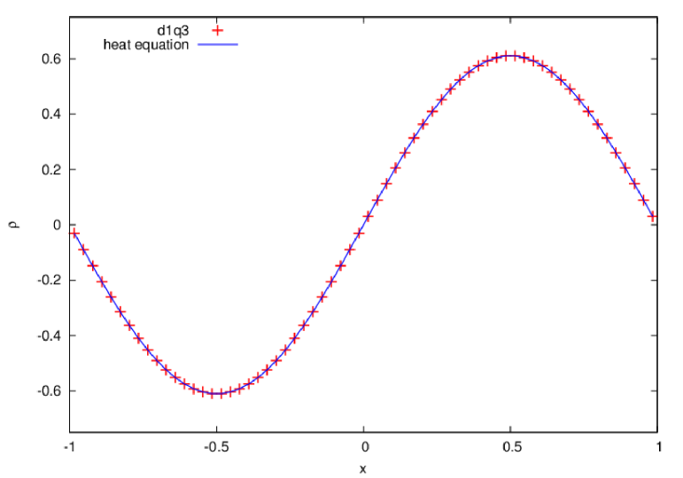
Figure 1: Sine wave at time $\,T=5\,$ computed with 64 mesh cells.

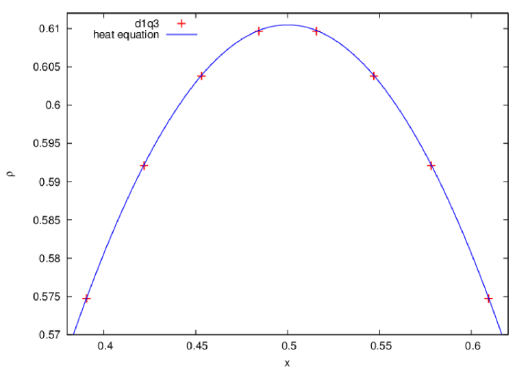
Figure 2: Sine wave computed with 64 mesh cells at time $\,T=5\,$; detail.

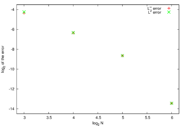
Figure 3: Numerical convergence to the diffusion equation (7).

It should be noted that the results are remarkably converged even for these relatively coarse meshes. For the most refined mesh used (64 mesh points, $\Delta x={1\over 32}$), the numerical results are almost indistinguishable from the exact solution, as presented in two successive magnifications in Fig. 2.

4)  An alternative convergence analysis

We now imagine that we wish to approximate the diffusion equation, Eq. (7), using the D1Q3 lattice Boltzmann model described previously. We suppose that the diffusion coefficient $\,\mu\,$ is fixed and that the mesh size $\,\Delta x\,$ tends to zero. Then from Eq. (8), the relaxation parameter $\,s_{J}\,$ can no longer be fixed and tends to zero according to the asymptotic prescription

(10) $$s_{J}\,=\,{{4+\alpha}\over{6\,\mu}}\,\lambda\,\Delta x\,+\,{\rm O}(\Delta x^{2})\,.\vspace*{-7pt}$$

The hypothesis used for deriving the diffusion model, Eqs. (7,8) is now violated, because the relaxation parameter $\,s_{J}\,$ is no longer a constant. Rather, it follows the asymptotic form

(11) $$s_{J}\,=\,s_{0}+s_{1}\,\Delta x+{\rm O}(\Delta x^{2})+\cdots,\vspace*{-7pt}$$

as suggested by one of us in earlier work on lattice-gas automata [2]. Moreover, we have

(12) $$s_{0}\,=\,0\,,\quad s_{1}={{4+\alpha}\over{6\,\mu}}\,\vspace*{-7pt}$$

for the case described in Eq. (10). Then the differential equation obtained in the asymptotic limit is no longer the diffusion equation Eq. (7), as discussed in the following proposition.

$\bullet$  Proposition 1.  An asymptotically acoustic model

We consider the D1Q3 lattice Boltzmann scheme defined by Eqs. (2,3,4,5,6). We make the hypothesis that the numerical velocity $\,\lambda\,$, defined in Eq. (1), and the relaxation coefficient $\,s_{e}\,$ used in the relaxation step Eq. (5), are constant as the spatial step $\,\Delta x\,$ tends to zero. Moreover, we suppose that the relation between the given diffusion coefficient $\,\mu\,$ and the relaxation coefficient $\,s_{J}\,$ follows the relation in Eq. (8). In other words, the relaxation coefficient $\,s_{J}\,$ admits the asymptotic hypotheses in Eqs. (11,12) with $\,s_{0}=0\,$ and $\,s_{1}={{4+\alpha}\over{6\,\mu}}$. Then, when $\,\Delta x\,$ tends to zero, the density $\,\rho\,$ and the momentum after relaxation $\,J^{*}\,$ obey the following acoustic model:

(13) $${{\partial\rho}\over{\partial t}}\,+\,{{\partial J^{*}}\over{\partial x}}\,=\,{\rm O}(\Delta x)\,,\quad{{\partial J^{*}}\over{\partial t}}\,+\,\lambda^{2}\,{{4+\alpha}\over{6}}\,{{\partial\rho}\over{\partial x}}\,+\,\lambda^{2}\,{{4+\alpha}\over{6\,\mu}}\,J^{*}(x,\,t)\,=\,{\rm O}(\Delta x)\,.\vspace*{-7pt}$$

$\bullet$  The proof of this result is given in the Appendix 1. The system Eq. (13) is an acoustic model with sound velocity $\,c_{0}=\lambda\,\sqrt{{4+\alpha}\over{6}}$. We see that we have dissipation of momentum with a zero-order operator. We have implemented a staggered finite-difference method named “HaWAY,” in reference to the authors Harlow and Welch [8], Arakawa [1] and Yee [13] who invented it in the mid 1960’s, for applications to fluid flow (“marker and cell”), geophysical sciences (“c-grid”) and electromagnetism (“finite difference time domain”), respectively. The details of this second-order numerical scheme are given in Appendix 2. This finite-difference approximation gives a correct second-order accurate solution of the system obtained by replacing the corrections $\,{\rm O}(\Delta x)\,$ by $\,0\,$ on the right-hand side of Eqs. (13).

5)  Additional numerical experiments

We next experiment with the diffusion of a Gaussian density profile with the D1Q3 lattice Boltzmann model defined in this work. The initial density profile is given by the relation

(14) $$\rho_{0}(x)={\rm exp}\Big{(}{\displaystyle-{{x^{2}}\over{4\,\mu}}}\,\Big{)}\quad{\rm with}\quad\,x\in\mathbb{R}\,.\vspace*{-7pt}$$

The other moments $\,J\,$ and $\,e\,$ are taken to be at equilibrium at $\,t=0$. Then the exact solution of the diffusion equation, Eq. (7), is obtained without difficulty:

(15) $$\rho(x,\,t)={{1}\over{\sqrt{1+t}}}\,\exp\Big{(}-{{x^{2}}\over{4\,\mu\,(1+t)}}\,\Big{)}\,,\quad x\in\mathbb{R}\,,\ t>0\,.\vspace*{-7pt}$$

We simulate this problem for $\,\mu=0.01\,$ and $\,0\leq t\leq T=5\,$ in a relatively large domain $\,-16\leq x\leq 16\,$ in order to avoid unwanted interactions of the diffusing Gaussian with the boundary. This has allowed us to employ an elementary periodic boundary condition at $x=\pm 16$, where all the fields have a value inferior to the smallest number that can be represented in floating-point arithmetic.

$\bullet$  At the macroscopic scale, we see in Fig. 4 that the numerical solution computed with the D1Q3 lattice Boltzmann scheme faithfully reproduces the exact solution Eq. (15) of the diffusion equation. After magnification by a factor of 100 (Fig. 5), the D1Q3 model simulates the acoustic-like system, Eq. (13), with better accuracy than it does the diffusion equation, Eq. (7). Fig. 6 shows that when the mesh is refined from $\,2^{6}=64\,$ to $\,2^{16}=65\,536\,$ vertices, the convergence towards the acoustic model seems reasonable, with an order of accuracy close to $1$. In other terms, the diference between the discrete solution of the D1Q3 model and the finite-difference simulation of the acoustic model goes to zero proportionally to the mesh size.

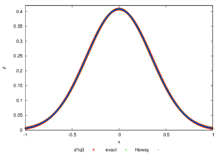
Figure 4: Gaussian a time $\,T=5$.

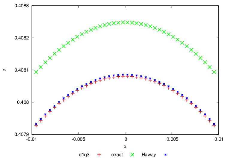
Figure 5: Detail of the Gaussian a time $\,T=5$.

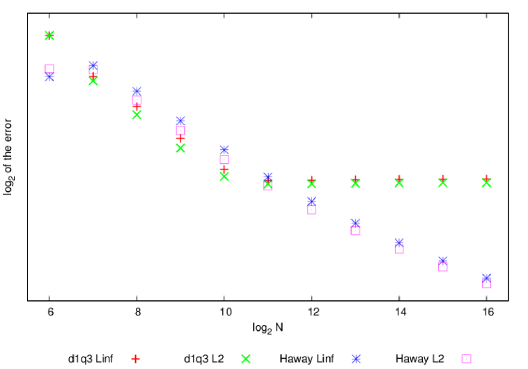
Figure 6: D1Q3 lattice Bolztmann scheme for diffusion; Gaussian at time = 5. Non- convergence towards the exact solution of the diffusion model Eq. (7) and convergence towards the acoustic model Eq. (13).

$\bullet$  Now we have what seems like a contradiction: Our first experiments for the sine wave show (see, e.g., Fig. 3) that the diffusion equation is a good reference mathematical model, whereas the acoustic model Eq. (13) is asymptotically correct for the Gaussian initial condition (see Fig. 6). We have performed simulations for the sine wave with much more refined meshes, and lattice sizes up to 4096. At the macroscopic scale, no difference is visible between the sine wave solution of the diffusion equation and the numerical result proposed by the lattice Boltzmann method (again, see Fig. 1). After magnification shown in Fig. 7, the difference between the exact solution of the diffusion equation and the D1Q3 solution is more important than the small discrepancy between the “HaWAY” numerical solution of the acoustic model, Eq. (13), and the lattice Boltzmann model.

$\bullet$  In Fig. 8, we have plotted the quadratic and uniform errors between the numerical solution obtained from the lattice Boltzmann model and the exact solution of the diffusion equation on one hand, and of the approximate solution (with a second-order scheme) of the acoustic model obtained after a first-order Taylor expansion analysis presented at Proposition 1 on the other hand. The lattice Boltzmann method gives an excellent approximation of the heat equation with the coarse meshes, as shown in Fig. 3 in Section 2. This good convergence quality cannot be explained by an asymptotic analysis. When the spatial step tends to zero, the lattice Boltzmann scheme gives a correct approximation of the acoustic model. Fig. 8 demonstrates that the convergence is first-order accurate in both norms.

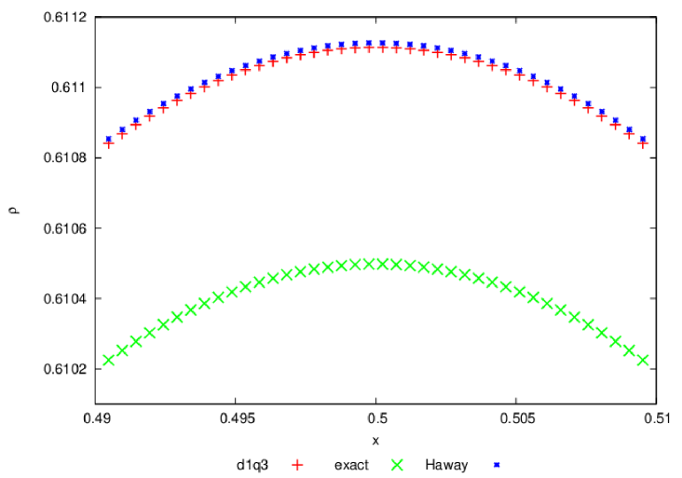
Figure 7: Sine wave at time = 5. Magnification of the solution around the extremal value.

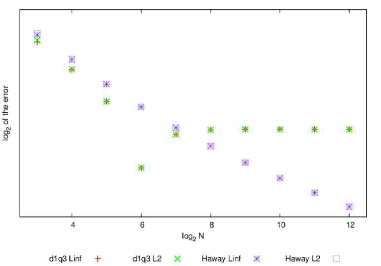
Figure 8: D1Q3 lattice Bolztmann scheme for diffusion; Sine wave at time = 5. Non- convergence towards the exact solution of the diffusion model Eq. (7) and convergence towards the acoustic model Eq. (13).

6)  Wave vectors analysis

We may also adopt the point of view of a spectral analysis of the lattice Boltzmann model, Eqs. (2,3,4,5,6). We search for a solution of the type

(16) $$f(x,\,t)\,=\,\exp\big{(}i\,k\,x\big{)}\,\,\exp\big{(}\zeta\,t\big{)}\,\begin{pmatrix}\varphi_{+}\cr\varphi_{0}\cr\varphi_{-}\end{pmatrix}\,.\vspace*{-7pt}$$

In one time step, we first transform the vector $\,f\,$ into moments. Then we relax the moments and return to the space of particles. Finally we advect the result according to Eq. (6) to recover the particle distribution. The collision step $\,m\longrightarrow m^{*}\,$ can be written in matrix form:

$$m^{*}\,=\,R\,\,m\,,\quad R\,=\,\begin{pmatrix}1&0&0\cr 0&1-s_{J}&0\cr\alpha\,{{\lambda^{2}}\over{2}}\,s_{e}&0&1-s_{e}\end{pmatrix}\vspace*{-6pt}$$

and the final advection step can be represented by the action of a diagonal matrix:

$$f(x,t+\Delta t)\,=\,A\,f^{*}(x,\,t)\,,\quad A\,=\,\begin{pmatrix}\exp(-i\,\xi)&0&0\cr 0&1&0\cr 0&0&\exp(i\,\xi)\end{pmatrix}\vspace*{-6pt}$$

with $\,\xi=k\,\Delta x$ . Then the vector $\,\varphi\,$ introduced in Eq. (16) must be a nontrivial solution of the following spectral problem:

$$\exp\big{(}\zeta\big{)}\,\varphi\,=\,A\,\,M^{-1}\,\,R\,\,M\,\varphi\,,\vspace*{-6pt}$$

with $\,\zeta=z\,\Delta t>0$. Then, denoting the identity matrix by $\,{\rm I}\,$, the dispersion relation takes the form

(17) $${\rm det}\,\big{[}\,A\,\,M^{-1}\,\,R\,\,M\,-\,\exp\big{(}\zeta\big{)}\,{\rm I}\,\big{]}\,=\,0\,.\vspace*{-7pt}$$

$\bullet$  We have performed an asymptotic analysis of the relation in Eq. (17) in the limit of a small relaxation coefficient $\,s_{J}$ (as in Eq. (10)), a small wave vector $\,\xi\,$ and with a small amplification factor $\,\zeta$:

(18) $$s_{J}\,=\,\varepsilon\,s_{1}\,,\quad\xi\,=\,\varepsilon\,\kappa\,,\quad\zeta\,=\,\varepsilon\,\omega\ ,\vspace*{-7pt}$$

where $\,\varepsilon\,$ is a small parameter that tends to zero. After some calculation, we obtain without difficulty

(19) $${\rm det}\,\big{[}\,A\,\,M^{-1}\,\,R\,\,M\,-\,\exp\big{(}\zeta\big{)}\,{\rm I}\,\big{]}\,=\,-s_{e}\,\Big{(}\omega^{2}\,+\,s_{1}\,\omega\,+\,{{4+\alpha}\over 6}\,\kappa\Big{)}\,\varepsilon^{2}\,+\,{\rm O}(\varepsilon^{3})\,.\vspace*{-7pt}$$

When $\,\kappa=0$, we recover the hydrodynamic mode with $\,\omega=0\,$ and a dissipative mode according to $\,\omega=-s_{1}$. When $\,\kappa\not=0$, we have to solve an equation of degree 2 made explicit in Eq. (19) at this order of accuracy. The discriminant of this equation becomes negative when

(20) $$\kappa\,\geq\,{{s_{1}}\over{2\,\sqrt{{4+\alpha}\over 6}}}\,.\vspace*{-7pt}$$

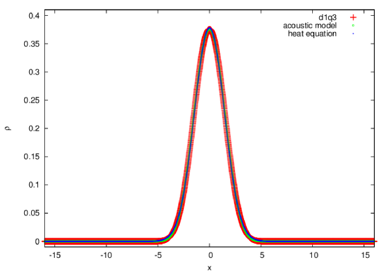
Figure 9: Gaussian, $\,\mu=0.15$. The heat equation is correctly approximated.

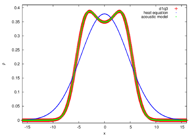
Figure 10: Gaussian, $\,\mu=1.5$. The propagation effects are clearly visible.

$\bullet$  We observe that the asymptotics associated with the limit $\,s_{J}\longrightarrow 0\,$ is questionable from a physical point of view. When establishing macroscopic partial differential equations it is assumed that internal degrees of freedom of the system under study evolve very “fast” compared to the macroscopic quantities. It is known (see, e.g., [4]) that $\,s_{J}\,$ is given by a ratio of the type $\,{{\Delta t}\over{\tau}}$. In the present case, the slow internal degrees of freedom evolve within times $\,\tau\approx{{\Delta t}\over{s}}$. So it is to be expected that the pure diffusion partial differential equation will not be accurate for very small values of $s$.

$\bullet$  In order to make this qualitative difference explicit, we have done two numerical experiments with the initial Gaussian profile given by Eq. (14). We use $2\,048$ mesh points and a final time $\,T=6\,$ after 384 iterations of the D1Q3 scheme. In the first experiment (Fig. 9), the diffusion $\,\mu\,$ is equal to $\,0.15\,$ so $\,s_{J}=0.050761\,$ wich satisfies Eq. (8). For the second experiment, all parameters are unchanged, except that $\,\mu=1.5\,$ and the relaxation coefficient $\,s_{J}=0.005195$ is much smaller. With this value of $\,s_{J}\,$ the expression, Eq. (20), is satisfied and the discriminant of the equation (19) is negative. The propagation effects are evident in Fig. 10. One may interpret the result: for small values of parameter $\,s$, the time between collisions is longer than the duration of the simulation, so particles move “ballistically”.

7)  Conclusion

We have described a curious convergence property of the D1Q3 lattice Boltzmann model, observed when trying to simulate a diffusion process with an acoustic scale. A new asymptotic analysis has been derived for this circumstance, and we have presented evidence of an asymptotic partial differential equation of acoustic type. We have observed analogous difficulties in two spatial dimensions, both for diffusion and Stokes flows. Overall results and physical interpretations will be given later, with comparison made to the phenomenon of viscoelasticity [6].

A natural question for future study is the generalization of this acoustic-type model to two or three spatial dimensions. Another is the application of this methodology to lattice Boltzmann models of fluid flow, using an acoustic scale while holding fixed the value of the viscosity.

Finally, it seems plausible that there is a link between the strange “first convergence” property noted in this work and the well known tendency of certain asymptotic series to converge at first, followed by divergence (see e.g. [7]). This would raise the question of exactly when the error is minimized, and what is an acceptable approximation of its value when it is minimal.

Acknowledgments

The authors thank Luc Mieussens who drew our attention to the interesting results obtained by Stéphane Dellacherie in [3].

Appendix 1  Proof of Proposition 1

We start from the time iteration, Eq. (6), and transfer it to the moments:

$$m_{k}(x,\,t+\Delta t)\,=\,\sum_{j\,\ell}\,M_{kj}\,\,M^{-1}_{j\ell}\,\,m_{\ell}^{*}(x-v_{j}\,\Delta t,\,t)\,.\vspace*{-6pt}$$

With the help of the tensor of momentum-velocity $\,\Lambda\,$ introduced in [4], defined according to

$$\Lambda_{k}^{\ell}\,=\,\sum_{j}\,M_{kj}\,\,v_{j}\,\,M^{-1}_{j\ell}\vspace*{-6pt}$$

and made explicit for our model as

(21) $$\Lambda\,=\,\begin{pmatrix}0&1&0\cr{2\over 3}\,\lambda^{2}&0&{1\over 3}\cr 0&\lambda^{2}&0\end{pmatrix}\,,\vspace*{-7pt}$$

we have

(22) $$m_{k}(x,\,t)\,+\,\Delta t\,{{\partial m_{k}}\over{\partial t}}\,+\,{\rm O}(\Delta t^{2})\,=\,m_{k}^{*}(x,\,t)\,-\,\Delta x\,\sum_{\ell}\,\Lambda_{k}^{\ell}\,{{\partial m_{\ell}^{*}}\over{\partial x}}\,+\,{\rm O}(\Delta x^{2})\,.\vspace*{-7pt}$$

$\bullet$  The first moment $\,m_{0}\equiv\rho\,$ is conserved (see Eq. (5)) and $\,\rho^{*}=\rho$. We deduce from Eq. (22) and the specific values of the first line of the matrix $\,\Lambda\,$ in Eq. (21) that

(23) $${{\partial\rho}\over{\partial t}}\,+\,{{\partial J^{*}}\over{\partial x}}\,=\,{\rm O}(\Delta x)\,\vspace*{-7pt}$$

and the first equation of Eq. (13) is established.

$\bullet$  The third moment $\,e\,$ is not at equilibrium and we have from the third relation of Eqs. (5,21,22):

$$s_{e}\,\big{(}e-e^{\rm eq}\big{)}\,\equiv\,e-e^{*}\,=\,-\Delta t\,{{\partial e}\over{\partial t}}\,-\,\Delta x\,\lambda^{2}\,{{\partial J^{*}}\over{\partial x}}\,+\,{\rm O}(\Delta x^{2})\,=\,{\rm O}(\Delta x)\,.\vspace*{-6pt}$$

The coefficient $\,s_{e}\,$ remains constant by hypothesis as $\,\Delta x\,$ tends to zero. Then this moment is close to the equilibrium:

$$e\,=\,{{\alpha}\over{2}}\,\lambda^{2}\,\rho\,+\,{\rm O}(\Delta x)\,,\quad e^{*}\,=\,{{\alpha}\over{2}}\,\lambda^{2}\,\rho\,+\,{\rm O}(\Delta x)\,\vspace*{-6pt}$$

and

(24) $${{\partial e^{*}}\over{\partial x}}\,=\,\lambda^{2}\,{{\alpha}\over{2}}\,{{\partial\rho}\over{\partial x}}\,+\,{\rm O}(\Delta x)\,.\vspace*{-7pt}$$

$\bullet$  The analysis for the second equation differs from what has been proposed previously in [4] because the moment $\,J\,$ and the same moment $\,J^{*}\,$ after relaxation are now not close to the equilibrium value $\,J^{\rm eq}=0$. More precisely, we have, due to the second relation of Eq. (5):

$$J\,=\,{{J^{*}}\over{1-s_{J}}}\,=\,\Big{(}1\,+\,{{4+\alpha}\over{6\,\mu}}\,\lambda\,\Delta x\,+\,{\rm O}(\Delta x^{2})\Big{)}\,J^{*}\,.\vspace*{-6pt}$$

Then $\displaystyle\quad J(x,\,t+\Delta t)\,=\,\Big{(}1\,+\,{{4+\alpha}\over{6\,\mu}}\,\lambda\,\Delta x\,+\,{\rm O}(\Delta x^{2})\Big{)}\,J^{*}(x,\,t+\Delta t)$

$\ \displaystyle\,=\,\Big{(}1\,+\,{{4+\alpha}\over{6\,\mu}}\,\lambda\,\Delta x\Big{)}\,J^{*}\,+\,\Delta t\,{{\partial J^{*}}\over{\partial t}}\,+\,{\rm O}(\Delta x^{2})$

$\ \displaystyle\,=\,J^{*}(x,\,t)\,+\,\Delta t\,{{\partial J^{*}}\over{\partial t}}\,+\,{{4+\alpha}\over{6\,\mu}}\,\lambda\,\Delta x\,J^{*}(x,\,t)\,+\,{\rm O}(\Delta x^{2})\,.$

We report this expression in the expansion Eq. (22), we substract $\,J^{*}(x,\,t)\,$ from both sides of the equation and we divide by $\,\Delta t$. Due to the previous result Eq. (24), we obtain:

$${{\partial J^{*}}\over{\partial t}}\,+\,{{4+\alpha}\over{6\,\mu}}\,\lambda^{2}\,J^{*}\,+\,{\rm O}(\Delta x)\,=\,-{2\over 3}\,\lambda^{2}\,{{\partial\rho}\over{\partial x}}\,-\,\lambda^{2}\,{{\alpha}\over{2}}\,{{\partial\rho}\over{\partial x}}\,+\,{\rm O}(\Delta x)\vspace*{-6pt}$$

and the second equation of Eqs. (13) is established. $\square$

Appendix 2  “HaWAY” staggered finite differences

We consider the acoustic model proposed in Eq. (13). With compact notation, we denote it here according to :

(25) $${{\partial\rho}\over{\partial t}}\,+\,{{\partial J}\over{\partial x}}\,=\,0\,,\quad{{\partial J}\over{\partial t}}\,+\,c_{0}^{2}\,{{\partial\rho}\over{\partial x}}\,+\,\Gamma\,J(x,\,t)\,=\,0\,.\vspace*{-7pt}$$

Given a spatial step $\,\Delta x\,$ and a time step $\,\Delta t$, we consider integer multiples of these parameters for the discretization of space and time. The density $\,\rho\,$ is approximated at semi-integer vertices in space and integer points in time whereas the momentum $\,J\,$ is approximated at integer nodes in space and semi-integer values in time:

(26) $$\rho\,\approx\,\rho^{n}_{k+1/2}\,,\quad J\,\approx\,J^{n+1/2}_{k}\,.\vspace*{-7pt}$$

The Figure 11 gives an illustration of this classical choice [1, 8, 13].

Figure 11: HaWAY grid for staggered finite differences.

$\bullet$  We discretize the first equation of Eqs. (25) with a two-point centered finite-difference schemes around the vertex $\,\big{(}(k+{1\over 2})\,\Delta x\,,\,(n+{1\over 2})\,\Delta t\big{)}$:

(27) $${{1}\over{\Delta t}}\,\big{(}\rho^{n+1}_{k+1/2}-\rho^{n}_{k+1/2}\big{)}\,+\,{{1}\over{\Delta x}}\,\big{(}J^{n+1/2}_{k+1}-J^{n+1/2}_{k}\big{)}\,=\,0\,.\vspace*{-7pt}$$

We use the same approach for the discretization of the second equation of Eqs. (25) around the node $\,\big{(}k\,\Delta x\,,\,n\,\Delta t\big{)}$:

(28) $${{1}\over{\Delta t}}\,\big{(}J^{n+1/2}_{k}-J^{n-1/2}_{k}\big{)}\,+\,{{1}\over{\Delta x}}\,\big{(}\rho^{n}_{k+1/2}-\rho^{n}_{k-1/2}\big{)}\,+\,\Gamma\,J^{n}_{k}\,=\,0\,.$$

We interpolate the momentum at integer vertices with a simple centered mean value:

$$J^{n}_{k}\,=\,{{1}\over{2}}\,\big{(}J^{n+1/2}_{k}+J^{n-1/2}_{k}\big{)}\,.\vspace*{-6pt}$$

We incorporate this expression into the relation Eq. (28) and we obtain

(29) $$\Big{(}{{1}\over{\Delta t}}+{{\Gamma}\over{2}}\,\Big{)}\,J^{n+1/2}_{k}\,+\,{{1}\over{\Delta x}}\,\big{(}\rho^{n}_{k+1/2}-\rho^{n}_{k-1/2}\big{)}\,=\,\Big{(}{{1}\over{\Delta t}}-{{\Gamma}\over{2}}\,\Big{)}\,J^{n-1/2}_{k}\,.\vspace*{-7pt}$$

The numerical scheme is now entirely defined for internal nodes. We have used periodic boundary conditions.

References

References

- [1] A. Arakawa. “Computational Design for Long-Term Numerical Integration of the Equations of Fluid Motion”, Journal of Computational Physics, vol. 1, p. 119-143, 1966.
- [2] B. Boghosian, W. Taylor. “Correlations and renormalization in lattice gases”, Phys. Rev. E, vol. 52, p. 510-554, 1995.
- [3] S. Dellacherie. “Construction and Analysis of Lattice Boltzmann Methods Applied to a 1D Convection-Diffusion Equation”, Acta Applicandae Mathematica, vol. 131, Issue 1, p. 69-140, 2014.
- [4] F. Dubois. “Equivalent partial differential equations of a Boltzmann scheme”, Computers and mathematics with applications, vol. 55, p. 1441-1449, 2008.
- [5] F. Dubois, P. Lallemand. “Towards higher order lattice Boltzmann schemes ”, J. Stat. Mech.: Theory and Experiment, P06006, 2009.
- [6] L. Giraud, D d’Humières, P. Lallemand. “A Lattice-Boltzmann Model for Visco-Elasticity”, International Journal of Modern Physics C, vol. 08, p. 805-815, 1997.
- [7] G.H. Hardy. Divergent Series, Oxford University Press, New York, 1949.
- [8] F.H. Harlaw, J.E.Welsch. “Numerical calculation of time-dependent viscous incompressible flow of fluid with a free surface”, Physics of Fluids, vol. 8, p. 2182-2189, 1965.
- [9] M. Hénon. “Viscosity of a Lattice Gas”, Complex Systems, vol. 1, p. 763-789, 1987.
- [10] D. d’Humières. “Generalized Lattice-Boltzmann Equations”, in Rarefied Gas Dynamics: Theory and Simulations, vol. 159 of AIAA Progress in Astronautics and Astronautics, p. 450-458, 1992.
- [11] P. Lallemand, L.-S. Luo. “Theory of the lattice Boltzmann method: Dispersion, dissipation, isotropy, Galilean invariance, and stability”, Physical Review E, vol. 61, p. 6546-6562, 2000.
- [12] S. Ubertini, P. Asinari, S. Succi. “Three ways to lattice Boltzmann: A unified time-marching picture”, Phys. Rev. E, vol. 81, 016311, 2010.
- [13] K. Yee. “Numerical solution of initial boundary value problems involving Maxwell’s equations in isotropic media”, IEEE Transactions on Antennas and Propagation, vol. 14, p. 302-307, 1966.