Normal and anomalous random walks of 2-d solitons

Abstract

Solitons, which describe the propagation of concentrated beams of light through nonlinear media, can exhibit a variety of behaviors as a result of the intrinsic dissipation, diffraction, and the nonlinear effects. One of these phenomena, modeled by the complex Ginzburg-Landau equation, are chaotic explosions, transient enlargements of the soliton that may induce random transversal displacements, which in the long run lead to a random walk of the soliton center. As we show in this work, the transition from non-moving to moving solitons is not a simple bifurcation but includes a sequence of normal and anomalous random walks. We analyze their statistics with the distribution of generalized diffusivities, a novel approach that has been used successfully for characterizing anomalous diffusion.

Powerful coherent laser light in crystals or fibers can suffer nonlinear interactions that prevent its divergence and foster stable propagation as a single entity: a soliton. In this theoretical work, we study solitons that have been found in experimental setups where energy is continuously injected to overcome dissipation. Using a simple mathematical model for the dynamics of the electromagnetic waves in the nonlinear media, we analyze the long term behavior of the center of the soliton (projected into a transversal plane) and characterize the statistics of the trajectories using mathematical concepts developed for random walks.

I Introduction

Localized waves that travel through space without major changes in their shape appear in several physical phenomenaDescalziClerc ; Liehr , for instance, hydrodynamicsKBS88 ; NAC90 , opticsTSW97 ; USM03 , and surface reactionsRJVE91 ; BBK15 . Their existence is explained as a balance between nonlinearity, dispersion, diffraction, and energy fluxesAkhmedievAnkiewicz . The name ‘dissipative soliton’ is reserved for those structures that share some properties with ‘classical solitons’ of integrable models (for instance the nonlinear Schrödinger equation), although they are not conservative. These dissipative solitons are either stationary, oscillating, or chaotic and may move with more or less fixed shape and velocity.

One of the peculiar phenomena of dissipative solitons are ‘explosions’SAA00 ; AST01 ; AS04 : transient enlargements of amplitude and size of the soliton induced by the chaotic internal dynamics without the need of external perturbations. These short-lived explosions do not destroy the soliton. Experimental evidence of explosions of solitons has been obtained in several experiments involving the propagation of strong light pulses in Ti:sapphire mode-locked lasers CSA02 and in double-clad ytterbium-doped fibers GA12 ; RBE15 ; RBE16 ; LLY16 ; LLX16 .

Recent work of the authorsCCDB12 ; CDAR16 ; CAR17 focussed on trajectories of solitons that can be described as random walks. The position of the soliton, as a result of spatial jumps with random orientations induced by explosions, has a probability density that spreads diffusively in the plane. We have shownCDAR16 how this diffusive behavior can be anomalous, i.e. the mean-squared displacement of the location of the soliton grows nonlinearly with time.

Anomalous diffusion has been observed in a large variety of natural and artificial systems, and in the last decades, a sophisticated mathematical framework has been developed MW65 ; KlafterSokolov ; MJC14 ; KlagesRadonsSokolov . The study of anomalous diffusion has made a fascinating progress, both theoretically and experimentally, and benefited from numerous reports outside the domain of Physics.

This article is a continuation of Ref. CDAR16, and has the following three objectives: (i) Describe the transition between no diffusion (soliton exploding in-place) and normal diffusion as a single parameter is varied. (ii) Understand the role of anomalous diffusion in the transition. (iii) Use new measures to describe different regimes of diffusion, particularly the distribution of generalized diffusivities introduced in Ref. AR13, in extension of the concepts of Ref. bauer2011, .

II The model

The basic model for the study of explosions of dissipative solitons is the complex cubic-quintic Ginzburg-Landau equation (CGL)ADA08 ; SAD08 :

$$\partial_{t}A=D\nabla_{\perp}^{2}A+\mu A+\beta|A|^{2}A+\gamma|A|^{4}A$$ (1)

on a two-dimensional spatial domain and subject to specified initial condition $A(x,y,0)$. The operator $\nabla_{\perp}^{2}=\partial_{x}^{2}+\partial_{y}^{2}$ is the isotropic Laplacian in two dimensions. Complex coefficients $D,\beta,\gamma$ are assumed constant and spatially uniform. The real coefficient $\mu$ (distance to the onset of linear instability) is also constant and uniform and is going to be used as our main bifurcation parameter. $D$ represents diffraction and spectral filtering; $\mu$ accounts for losses; $\beta$ represents cubic nonlinear gain and Kerr effect; and $\gamma$ is the quintic nonlinear gain.

This model is relevant for wide aperture lasers, vertical external cavity semiconductor devices, and multimode optical fibers made of erbium doped glassWRCW15 ; WCW17 .

There are wide regions of combinations of parameters $(\mu,D,\beta,\gamma)$ where solutions can be localized in the plane with exponential tails that decay independently of the domain size $L$.

In this article, we used: $\beta=1+0.8\ \mathrm{i},\gamma=-0.1-0.6\ \mathrm{i},D=0.125+0.5\ \mathrm{i}$. We are interested in solutions that have shapes similar to a two-dimensional soliton. As it was mentioned in the Introduction, these solitons exhibit different behaviors: stationary, pulsating, or explosive. Explosive solitons experience infinite sequences of symmetric and asymmetric explosions. As it was found in Ref. CDAR16, , only the latter induce diffusive behavior but the former are relevant for the statistical properties.

The two-dimensional CGL, Eq. (1), was integrated from a localized initial condition using a split-step Fourier method. With the exception of $\mu$, all other parameters were kept fixed in all the simulations reported here.

The simulations were carried out using a $256\times 256$ spatial grid of size $dx\times dy=0.2\times 0.2$. The time discretization was $dt=0.005$, and the runs typically involved $2\times 10^{7}$ iterations, so the total time was $T=10^{5}$, so several thousands of explosions were registered in each run.

We checked our results using a finer spatial grid $512\times 512$ ($dx$ was halved so $dt$ was divided by 4 to respect the numerical accuracy) that the results were not artefacts of the spatial or temporal discretizations. The spatial power spectrum converged exponentially fast, so higher modes can be considered irrelevant.

Our codes were implemented on graphical processing units using the PyOpenCL library developed by Andreas Klöckner pycuda .

III Effective diffusion of solitons

Spatial diffusion is induced by random asymmetric explosions of the soliton that take place intermittently as a result of its chaotic dynamics. The sensitive dependence on initial conditions, typical for chaotic systems, implies that the precise timing of the explosions, their symmetry, and their spatial directions seem to be random.

We have foundCCDB12 ; CDAR16 that there are several regimes with significative differences. First there is a regime for values of $\mu\leq-0.40$, where all explosions are perfectly symmetric and the location of the soliton remains stationary. Then there is another regime for values of $\mu\geq-0.30$, where most explosions are asymmetric and lead to a random walk of the location of the soliton that obeys the statistics of Brownian motion: uncorrelated jumps of finite size and finite waiting times between the jumps. But there is an intermediate range, $-0.40<\mu<-0.30$, where one can find for some range of values of $\mu$ a third alternative: long sequences of symmetric explosions interspersed with some asymmetric explosions. As the time between asymmetric explosions can be arbitrarily long in the sense that they follow a heavy-tailed distribution with infinite mean, the resultant random walk has statistics different from Brownian motion and falls in the class of anomalous diffusion, more specifically, subdiffusion, which can be modeled by a subdiffusive continuous time random walk (CTRW).

To quantify the differences between these regimes, we define the coordinates of the ‘center of mass’ of the soliton:

$$x_{\mathrm{cm}}(t)\stackrel{{\scriptstyle\mathrm{def}}}{{=}}\frac{L}{2\pi}\mathrm{arg}\left(\int|A|^{2}\exp\left(\frac{\mathrm{i}2\pi x}{L}\right)\,\mathrm{d}x\,\mathrm{d}y\right)$$

and analogously for $y_{\mathrm{cm}}(t)$. These definitions respect the periodicity of the domain and can be used to define the vector center of mass:

$$\bm{r}(t)\stackrel{{\scriptstyle\mathrm{def}}}{{=}}\left(\begin{array}[]{c}x_{\mathrm{cm}}(t)\\ y_{\mathrm{cm}}(t)\end{array}\right)$$

(in the following, we will drop the subscript ‘cm’).

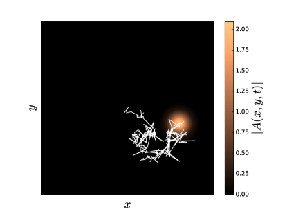
Figure 1: The white trajectory is an example of the chaotic evolution of the center $(x(t),y(t))$ of the soliton over a time $T=10^{5}$ as a result of repeated asymmetric explosions that lead to spatial shifts in random directions. The trajectory, initialized at the center of the square domain, is superimposed to a density plot of the absolute value of the soliton amplitude $A(x,y,t)$ at the final time $t=T$.

In Fig. 1, we plot the 2-d soliton and the trajectory of its center of mass. It was generated from an initial condition, where we added some small spatial noise to a Gaussian pulse, by integrating the deterministic law represented by Eq. (1). Asymmetric explosions induce random jumps. As it was mentioned above, the coexistence of symmetric and asymmetric explosions may lead to anomalous random walks if the mean time between asymmetric explosions is infinite.

The basic quantity that is used to characterize diffusive motion is the mean-squared displacement (MSD), which can be defined either as ensemble average or as time average.

The ensemble-averaged squared displacement (EASD) is defined by

$$\langle||\Delta\bm{r}(\tau)||^{2}\rangle_{\mathrm{E}}\stackrel{{\scriptstyle\mathrm{def}}}{{=}}\lim_{N\rightarrow\infty}\frac{1}{N}\sum_{i=1}^{N}||\bm{r}_{i}(\tau)||^{2}$$ (2)

assuming $\bm{r}_{i}(0)=0$. In Fig. 2, we plot such averages obtained from ensembles of $N=64$ independent realizations for a variety of values of $\mu$ at time $\tau=10^{4}$. The plot shows, as we sweep the interval with increments of size $\Delta\mu=0.01$, a general trend of larger EASD for larger $\mu$, but in the intermediate regime for $\mu=-0.380,-0.350,-0.320$, there are some points with very small displacements. They may correspond to static solitons or some other form of diffusion.

The EASD asympotically increases with a power law,

$$\langle||\Delta\bm{r}(\tau)||^{2}\rangle_{\mathrm{E}}\simeq\langle D_{\alpha}\rangle_{\mathrm{E}}\,\tau^{\alpha}\quad(\tau\rightarrow\infty),$$ (3)

where $\langle D_{\alpha}\rangle_{\mathrm{E}}$ is the generalized diffusion coefficient. The exponent $\alpha$ seems to be 1 for most values of $\mu$, that indicates normal diffusion and is consistent with the shape of the trajectories. But, as we will see, in some cases inside the intermediate regime, there are indications of anomalous diffusion, $\alpha\neq 1$. Although the exponent $\alpha$ is the primary signal of anomalous diffusion, finite simulation times and the limited number of trajectories make its estimation difficult.

The time-averaged squared displacement (TASD) of an individual trajectory is defined by

$$\langle||\Delta\bm{r}(\tau)||^{2}\rangle_{\mathrm{T}}\stackrel{{\scriptstyle\mathrm{def}}}{{=}}\frac{1}{T-\tau}\int_{0}^{T-\tau}||\bm{r}(t+\tau)-\bm{r}(t)||^{2}\,\mathrm{d}t.$$ (4)

This quantity is not necessarily ‘reproducible’ even for long simulation times $T$, i.e. independent realizations (from different initial conditions) may give very different values of $\langle||\Delta\bm{r}(\tau)||^{2}\rangle_{\mathrm{T}}$.

The scaling of the TASD often turns out to be quite different from the EASD. The TASD gives a result for each independent trajectory. Our results for all $\mu$ indicate that for long $T$ and $\tau<T$, the TASD grows linearly with time,

$$\langle||\Delta\bm{r}(\tau)||^{2}\rangle_{\mathrm{T}}\simeq\langle D_{1}\rangle_{\mathrm{T}}\ \tau~{}.$$ (5)

Now as we will show, for finite $T$, the proportionality coefficient of the TASD is a random variable. In the case of normal difusion, there is a small scatter that gets smaller for larger values of $T$. In the case of anomalous diffusion, this proportionality coefficient varies wildly from realization to realization (the values span several orders of magnitude) and these fluctuations remain, even for infinite $T$. Fig. 3 shows the large width of these distributions.

The last plot also shows (with horizontal bars) the ensemble averages of the TASD:

$$\langle\langle||\Delta\bm{r}(\tau)||^{2}\rangle_{\mathrm{T}}\rangle_{\mathrm{E}}=\lim_{N\rightarrow\infty}\frac{1}{N}\sum_{i=1}^{N}\langle||\Delta\bm{r}_{i}(\tau)||^{2}\rangle_{\mathrm{T}}.$$

Comparing Fig. 2 with Fig. 3 and the observed scaling relations (using finite $T$ and $\tau<T$), there are some indications that for some values of $\mu$ :

$$\langle\langle||\Delta\bm{r}(\tau)||^{2}\rangle_{\mathrm{T}}\rangle_{\mathrm{E}}\neq\langle||\Delta\bm{r}(\tau)||^{2}\rangle_{\mathrm{E}}~{}.$$

The last inequality receives the name ‘weak ergodicity breaking’ and leads to several counter-intuitive effectsMJC14 .

$\mu$		Behavior
-0.40		no diffusion
-0.39		anomalous
-0.38		anomalous
-0.37		normal
-0.36		no diffusion
-0.35		anomalous
-0.34		normal
-0.33		no diffusion
-0.32		not clear
-0.31		no diffusion
-0.30		normal

Table 1: Different behaviours reveal transition between non-moving soliton to walking solitons as the parameter $\mu$ is increased. In the intermediate range, small windows of anomalous diffusion are interspersed with non-moving and normal diffusion.

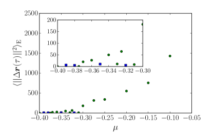
Figure 2: Summary of behaviors of EASD defined by Eq. (2) evaluated at $\tau=10^{4}$. For $\mu<-0.4$, the location of the soliton remains static. For $\mu>-0.3$, the location of the soliton describes a normal random walk. In the intermediate range, as indicated in the small inset, diffusive motion alternates with regimes of no diffusion and with anomalous diffusion (indicated by blue squares).

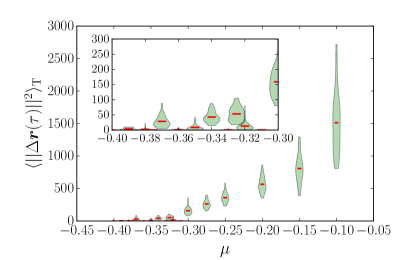
Figure 3: Summary of behaviors of TASD defined by Eq. (4) evaluated for $\tau=10^{4},T=10^{5}$. For each value of $\mu$, the vertical shape indicates the distribution of values that $\langle||\Delta\bm{r}(\tau)||^{2}\rangle_{\mathrm{T}}$ takes over the realizations. Red horizontal bars indicate the ensemble average of $\langle||\Delta\bm{r}(\tau)||^{2}\rangle_{\mathrm{T}}$. Anomalous cases show distributions that are concentrated not far from zero.

In the following, we focus our attention into two very different scenarios. We will show that the exponent $\alpha$ extracted from EASD is hard to measure accurately, and it is far better to look at the distribution of TASD, in particular, the distribution of $\langle D_{1}\rangle_{\mathrm{T}}$.

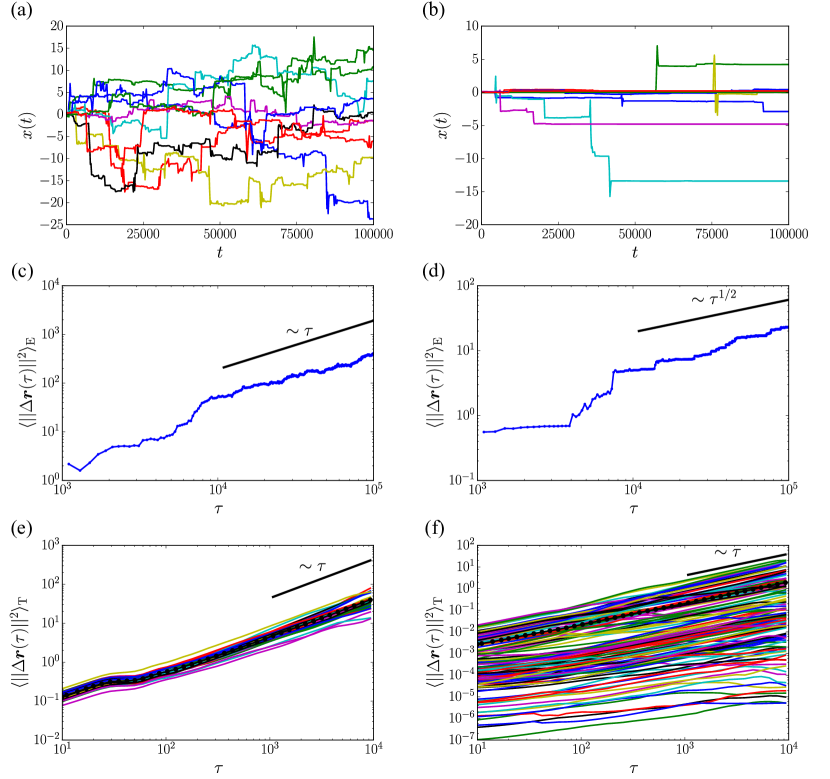
Figure 4: Comparison of two different diffusive behaviors of the $x$-coordinate of the center of mass of solitons that evolve in time according to Eq. (1). Left column corresponds to $\mu=-0.34$ and shows normal diffusion: $\langle||\Delta\bm{r}(\tau)||^{2}\rangle_{\mathrm{E}}$ grows linearly with time and $\langle||\Delta\bm{r}(\tau)||^{2}\rangle_{\mathrm{T}}$ show up as several straight lines with similar location. Right column corresponds to $\mu=-0.38$ and shows anomalous diffusion: $\langle||\Delta\bm{r}(\tau)||^{2}\rangle_{\mathrm{E}}$ grows with time following a power-law and $\langle||\Delta\bm{r}(\tau)||^{2}\rangle_{\mathrm{T}}$ show up as several straight lines with the same slope but at very different locations.

For $\mu=-0.340$ (left column in Fig. 4), all explosions are asymmetric and have independent directions. The soliton is at rest only for short periods of time. The resulting diffusion looks normal according to both ensemble-averaged and time-averaged squared displacements: EASD grows proportionally with time (exponent 1 in the log-log plot), and for the TASD, the vertical position of the curve in log-log plot (that captures the coefficient $\langle D_{1}\rangle_{\mathrm{T}}$) indicates that the spread between realizations is small (approaches zero for longer $T$). As ensemble and time averages coincide, the process can be considered ergodic.

For $\mu=-0.380$ (right column in Fig. 4), explosions can be asymmetric or symmetric. Long time intervals with only symmetric explosions show up as horizontal segments, and for large $t$, the probability of being at one of these waiting times grows. The exponent $\alpha<1$ in the EASD captures the presence of very long waiting times. The greater variability of the TASD among individual trajectories also indicates anomalous diffusion. Although the individual TASDs show linear growth with time-lag, their slopes are quite different, i.e. the diffusion coefficient $\langle D_{1}\rangle_{\mathrm{T}}$ is a random variable.

In Ref. CDAR16, , a more systematic way to analyze the scatter of the individual realizations was used based on the distribution of the normalized time-averaged squared-displacementhe2008 :

$$\xi\stackrel{{\scriptstyle\mathrm{def}}}{{=}}\frac{\langle||\Delta\bm{r}(\tau)||^{2}\rangle_{\mathrm{T}}}{\langle\langle||\Delta\bm{r}(\tau)||^{2}\rangle_{\mathrm{T}}\rangle_{\mathrm{E}}}.$$

The variance of $\xi$ quantifies ergodicity breaking in the limit of $T\rightarrow\infty$. In the case of normal diffusion, the distribution of $\xi$ is monomodal with a width that can be predicted analytically and vanishes for long $T$. In the case of a subdiffusive continuous time random walk, $\xi$ follows the Mittag-Leffler distribution with a width that does not vanish for long $T$.

IV Distribution of generalized diffusivities

Another mathematical tool, which can be used to analyze diffusion processes, is the distribution of generalized diffusivities (DOGD)AR13 ; AR14 ; Albers , which captures the fluctuations of generalized diffusivities defined as scaled squared displacements, $D_{\beta}(\tau)=||\Delta\bm{r}(\tau)||^{2}/\tau^{\beta}$. The advantages of the DOGD are that it obviously contains more information than the MSD, but contrary to the propagator, it is always a one-dimensional distribution and, therefore, simple to visualize. Furthermore, in contrast to the propagator, by choosing an appropriate value of the scaling exponent $\beta$, the DOGD may become stationary, i.e. independent of $\tau$. Especially, if $\beta$ is equal to the exponent of the asymptotic increase of the MSD, the mean value of the DOGD is equal to the prefactor of the asymptotic increase of the MSD, i.e. the generalized diffusion coefficient. The freedom to choose an exponent $\beta$ and a time frame $\tau$ can be used to reveal non-trivial pieces of the process dynamics.

The distribution of generalized diffusivities obtained as ensemble average is defined by

$$p_{\beta}^{\mathrm{E}}(D,\tau)\stackrel{{\scriptstyle\mathrm{def}}}{{=}}\left\langle\delta\left(D-\frac{||\bm{r}(\tau)-\bm{r}(0)||^{2}}{\tau^{\beta}}\right)\right\rangle_{\mathrm{E}},$$ (6)

where, as already mentioned, $\beta$ can be selected arbitrarily.

The distribution of generalized diffusivities obtained as time average from an individual realization of the process is defined by

$$p_{\beta}^{\mathrm{T}}(D,\tau)\stackrel{{\scriptstyle\mathrm{def}}}{{=}}\left\langle\delta\left(D-\frac{||\bm{r}(t+\tau)-\bm{r}(t)||^{2}}{\tau^{\beta}}\right)\right\rangle_{\mathrm{T}}.$$ (7)

If the generalized diffusion coefficient obtained from the TASD, which is just the first moment of the distribution $p_{\beta}^{\mathrm{T}}(D,\tau)$, is a random variable, the distribution $p_{\beta}^{\mathrm{T}}(D,\tau)$ must be random itself. Of course, this random distribution can be averaged over an ensemble of such distributions.

Both distributions can be computed analytically (or at least approximated by analytic expressions) in the situations that are relevant in the present context (full details of these derivations are presented in Ref. Albers, ).

• For a two-dimensional normal diffusion process, which is ergodic with respect to the squared displacements, we get for both definitions of the DOGD:

  $$p_{\beta}^{\mathrm{E}}(D,\tau) =\langle p_{\beta}^{\mathrm{T}}(D,\tau)\rangle_{\mathrm{E}}=p_{\beta}(D,\tau)$$

  $$=\int\delta\left(D-\frac{||\bm{r}||^{2}}{\tau^{\beta}}\right)\,p(\bm{r},\tau)d^{2}\bm{r},$$ (8)

  where

  $$p(\bm{r},\tau)=\frac{1}{2\pi\langle D_{1}\rangle\tau}\exp\left(-\frac{||\bm{r}||^{2}}{2\langle D_{1}\rangle\,\tau}\right)$$ (9)

  is the result for the propagator $\langle\delta(\bm{r}-\bm{r}(\tau))\rangle_{\mathrm{E}}$ of the process and $\langle D_{1}\rangle$ denotes the diffusion coefficient. We obtain

  $$p_{\beta}(D,\tau)=\frac{1}{2\langle D_{1}\rangle\tau^{1-\beta}}\exp\left(-\frac{D}{2\langle D_{1}\rangle\tau^{1-\beta}}\right).$$ (10)

  The first moment of $p_{\beta}(D,\tau)$ satisfies $\langle D_{\beta}(\tau)\rangle=\langle D_{1}\rangle\,\tau^{1-\beta}$. For the selection $\beta=1$, $p_{1}(D)$ does not depend on $\tau$, and one can verify that $\langle D_{1}\rangle$ is the first moment of $p_{1}(D)$.

• For a subdiffusive continuous random walk characterized by exponent $\alpha<1$ and in the limit of large $\tau$, the DOGD can be computed from the propagator, which can be represented in terms of the Fox H-functionSW89 :

  $$p(\bm{r},\tau)\simeq\frac{C}{\pi}\tau^{-\alpha}H^{2,0}_{1,2}\biggl{[}C\tau^{-\alpha}||\bm{r}||^{2}\biggl{|}{\scriptstyle\begin{array}[]{l}(1-\alpha,\alpha)\\ (0,1),(0,1)\end{array}}\biggr{]},$$ (11)

  where $C=[\langle D_{\alpha}\rangle_{\mathrm{E}}\Gamma(1+\alpha)]^{-1}$. Then the DOGD obtained from an ensemble of trajectories for the selection $\beta=\alpha$ is given by

  $$p_{\alpha}^{\mathrm{E}}(D,\tau)\simeq CH^{2,0}_{1,2}\biggl{[}CD\biggl{|}{\scriptstyle\begin{array}[]{l}(1-\alpha,\alpha)\\ (0,1),(0,1)\end{array}}\biggr{]}.$$ (12)

  One can show that the distribution $p_{1}^{\mathrm{T}}(D,\tau)$ is a linear combination of a singular part $\delta(D)$ caused by the long waiting times and a continuous part described by a Fox H-function. The weights of the two parts are random and depend on the random generalized diffusion coefficient $\langle D_{1}\rangle_{\mathrm{T}}$. The ensemble average of the distribution $p_{1}^{\mathrm{T}}(D,\tau)$ then takes the form:

  $$\langle p_{1}^{\mathrm{T}}(D,\tau)\rangle_{\mathrm{E}}\simeq\left(1-\frac{1}{\Gamma(2-\alpha)\Gamma(\alpha+1)}\left(\frac{\tau}{T}\right)^{1-\alpha}\right)\delta(D)\\ +\frac{C}{\Gamma(\alpha+1)}\left(\frac{\tau}{T}\right)^{1-\alpha}\tau^{1-\alpha}H^{2,0}_{1,2}\Biggl{[}CD\tau^{1-\alpha}\Biggl{|}\begin{array}[]{l}(2-2\alpha,\alpha)\\ (0,1),(0,1)\end{array}\Biggr{]}.$$ (13)

In Appendix A, it is shown how the Fox H-function can be transformed into a Meijer G-function. Furthermore, Appendix B provides asymptotic expansions of the Fox H-function.

Comparisons between the DOGD from the soliton’s trajectories ($\mu=0.34$ and $\mu=0.38$) and the analytical predictions for each regime are presented in Fig. 5. For $p_{\beta}^{\mathrm{E}}(D,\tau)$, we use the characteristic exponent $\beta=1$ for the normal random walk, and $\beta=\alpha$ for the anomalous (subdiffusive) random walk. For $\langle p_{\beta}^{\mathrm{T}}(D,\tau)\rangle_{\mathrm{E}}$, we use $\beta=1$ for both regimes.

Despite the small number of trajectories, we can appreciate how the analytical expressions of the DOGD in both forms (and without any further adjustment of parameters) capture two distinct features of anomalous diffusion, a considerable probability of jumps much larger than the average and long periods of time with very little displacement. These features are consistent with the soliton’s data and provide another way of identifying the regime.

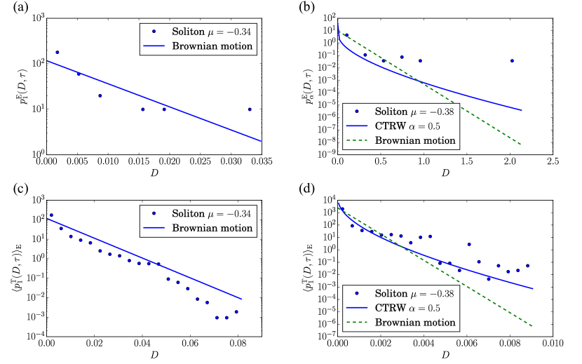
Figure 5: Comparison of two different diffusive behaviors using the distributions of generalized diffusivities defined by Eqs. (6) and (7) and evaluated with soliton’s data (blue points). We used $\tau=10^{4},T=10^{5}$. For each value of $\mu$, 64 slightly different initial conditions were used for the integration of the soliton’s trajectories. (a,c) DOGDs for $\mu=-0.340$ (normal diffusion). Despite that the small number of realizations prevented ensemble averages to converge, we obtained reasonable agreement with Eq. (10) with $\beta=1$ deduced from Brownian motion (solid blue line). (b,d) DOGDs for $\mu=-0.380$ (anomalous diffusion). In (b) we obtained good agreement with Eq. (12) deduced from subdiffusive CTRW with exponent $\alpha=1/2$ (blue solid curve) that captures the curvature induced by anomalous diffusion. We also show for comparison the distribution Eq. (10) of Brownian motion evaluated with $\beta=1/2$ (dashed green curve). In (d) there is good agreement with Eq. (13). We also show for comparison the distribution Eq. (10) evaluated with $\beta=1$ (dashed green curve).

V Conclusions

In this work, we explored the erratic trajectories of two-dimensional dissipative solitons modeled by the complex Ginzburg-Landau equation, relevant in nonlinear optics and other fields of physics.

In particular, we focused into the transition between the static soliton and the normally diffusing soliton as one parameter of the model was varied. The trajectories of the solitons can be described by a random walk, but in some cases they may show features that are quite different from what one could expect from a normal random walk or the Brownian process. The transition is not simple as indicated by nontrivial phenomena in an intermediate range of parameters.

In this work, we have used the ensemble-averaged squared displacement and the time-averaged square displacement as basic mathematic tools. The concept of the distribution of generalized diffusivities, recently introduced by some of the authors, extended the analysis possibilities of the squared displacements and allowed us to make comparisons between soliton’s data and analytic predictions.

For the anomalous regime, the distributions of generalized diffusivities showed a direct effect of long periods of time when the soliton exploded symmetrically and thus remained basically static.

Appendix A Transformation of the Fox H-function into a Meijer G-function

In this appendix, we demonstrate with four examples how the Fox H-function for rational values of its parameters can be transformed into the Meijer G-function (tabulated in Ref. 25 and implemented in the software Mathematica and the Python library mpmath), allowing plots of our analytical results.

Our first example occurs in the context of the distribution of generalized diffusivities $p^{E}_{\alpha}(D,\tau)$ obtained from an ensemble of subdiffusive CTRW trajectories in a two-dimensional space for $\alpha=1/2$:

$$H^{2,0}_{1,2}\Biggl{[}x\Biggl{|}\begin{matrix}(\frac{1}{2},\frac{1}{2})\\ (0,1),(0,1)\end{matrix}\Biggr{]} =\frac{1}{2\pi\mathrm{i}}\int_{\mathcal{C}}\frac{\Gamma(u)\Gamma(u)}{\Gamma(\frac{1}{2}+\frac{u}{2})}\>x^{-u}\>\mathrm{d}u$$

$$=\frac{1}{4\pi}H^{3,0}_{0,3}\Biggl{[}\frac{x}{4}\Biggl{|}\begin{array}[]{l}\text{---}\\ (0,\frac{1}{2}),(0,\frac{1}{2}),(\frac{1}{2},\frac{1}{2})\end{array}\Biggr{]}$$ (16)

$$=\frac{1}{2\pi}H^{3,0}_{0,3}\Biggl{[}\left(\frac{x}{4}\right)^{2}\Biggl{|}\begin{array}[]{l}\text{---}\\ (0,1),(0,1),(\frac{1}{2},1)\end{array}\Biggr{]}$$ (19)

$$=\frac{1}{2\pi}G^{3,0}_{0,3}\Biggl{[}\left(\frac{x}{4}\right)^{2}\Biggl{|}\begin{array}[]{l}\text{---}\\ 0,0,\frac{1}{2}\end{array}\Biggr{]}$$ (22)

Here, we used the definition of the Fox H-function (Eq. (1.2) and Eq. (1.3) in Ref. 25), the duplication formula of the Gamma function (Eq. (1.59) in Ref. 25),

$$\Gamma(u)=\Gamma\left(\frac{u}{2}\right)\,\Gamma\left(\frac{1}{2}+\frac{u}{2}\right)\,\frac{2^{u-1}}{\sqrt{\pi}}$$

so the integrand

$$\frac{\Gamma(u)\Gamma(u)}{\Gamma(\frac{1}{2}+\frac{u}{2})}=\Gamma\left(\frac{u}{2}\right)\,\Gamma\left(\frac{u}{2}\right)\,\Gamma\left(\frac{1}{2}+\frac{u}{2}\right)\,\frac{2^{2u}}{4\pi}$$

and the definition of the Meijer G-function (Eq. (1.112) in Ref. 25).

The second example appears in the context of the distribution of generalized diffusivities $p^{T}_{1}(D,\tau)$ obtained as time average from one single-particle trajectory of a two-dimensional, subdiffusive CTRW for $\alpha=1/2$:

$$H^{2,0}_{1,2}\Biggl{[}x\Biggl{|}\begin{array}[]{l}(1,\frac{1}{2})\\ (0,1),(0,1)\end{array}\Biggr{]} =\frac{1}{2\pi\mathrm{i}}\int_{\mathcal{C}}\frac{\Gamma(u)\Gamma(u)}{\Gamma(1+\frac{u}{2})}\>x^{-u}\>\mathrm{d}u$$ (25)

$$=\frac{1}{4\pi}H^{4,0}_{1,4}\Biggl{[}\frac{x}{4}\Biggl{|}\begin{array}[]{l}(1,\frac{1}{2})\\ (0,\frac{1}{2}),(0,\frac{1}{2}),(\frac{1}{2},\frac{1}{2}),(\frac{1}{2},\frac{1}{2})\end{array}\Biggr{]}$$ (28)

$$=\frac{1}{2\pi}H^{4,0}_{1,4}\Biggl{[}\left(\frac{x}{4}\right)^{2}\Biggl{|}\begin{array}[]{l}(1,1)\\ (0,1),(0,1),(\frac{1}{2},1),(\frac{1}{2},1)\end{array}\Biggr{]}$$ (31)

$$=\frac{1}{2\pi}G^{4,0}_{1,4}\Biggl{[}\left(\frac{x}{4}\right)^{2}\Biggl{|}\begin{array}[]{l}1\\ 0,0,\frac{1}{2},\frac{1}{2}\end{array}\Biggr{]}$$ (34)

For this calculation, we used the same methods as in the first example.

The third and the fourth examples correspond to the first two examples, but now for $\alpha=3/4$:

$$H^{2,0}_{1,2}\Biggl{[}x\Biggl{|}\begin{array}[]{l}(\frac{1}{4},\frac{3}{4})\\ (0,1),(0,1)\end{array}\Biggr{]} =\frac{1}{2\pi\mathrm{i}}\int_{\mathcal{C}}\frac{\Gamma(u)\Gamma(u)}{\Gamma(\frac{1}{4}+\frac{3u}{4})}\>x^{-u}\>\mathrm{d}u$$ (37)

$$=\frac{\sqrt[4]{3}}{(4\pi)^{2}}H^{7,0}_{2,7}\Biggl{[}\frac{\sqrt[4]{27}}{16}x\Biggl{|}\begin{array}[]{l}(\frac{1}{12},\frac{1}{4}),(\frac{5}{12},\frac{1}{4})\\ (0,\frac{1}{4}),(0,\frac{1}{4}),(\frac{1}{4},\frac{1}{4}),(\frac{1}{4},\frac{1}{4}),(\frac{1}{2},\frac{1}{4}),(\frac{1}{2},\frac{1}{4}),(\frac{3}{4},\frac{1}{4})\end{array}\Biggr{]}$$ (40)

$$=\frac{\sqrt[4]{3}}{(2\pi)^{2}}H^{7,0}_{2,7}\Biggl{[}\left(\frac{\sqrt[4]{27}}{16}x\right)^{4}\Biggl{|}\begin{array}[]{l}(\frac{1}{12},1),(\frac{5}{12},1)\\ (0,1),(0,1),(\frac{1}{4},1),(\frac{1}{4},1),(\frac{1}{2},1),(\frac{1}{2},1),(\frac{3}{4},1)\end{array}\Biggr{]}$$ (43)

$$=\frac{\sqrt[4]{3}}{(2\pi)^{2}}G^{7,0}_{2,7}\Biggl{[}\left(\frac{\sqrt[4]{27}}{16}x\right)^{4}\Biggl{|}\begin{array}[]{l}\frac{1}{12},\frac{5}{12}\\ 0,0,\frac{1}{4},\frac{1}{4},\frac{1}{2},\frac{1}{2},\frac{3}{4}\end{array}\Biggr{]}$$ (46)

$$H^{2,0}_{1,2}\Biggl{[}x\Biggl{|}\begin{array}[]{l}(\frac{1}{2},\frac{3}{4})\\ (0,1),(0,1)\end{array}\Biggr{]} =\frac{1}{2\pi\mathrm{i}}\int_{\mathcal{C}}\frac{\Gamma(u)\Gamma(u)}{\Gamma(\frac{1}{2}+\frac{3u}{4})}\>x^{-u}\>\mathrm{d}u$$ (49)

$$=\frac{1}{(4\pi)^{2}}H^{7,0}_{2,7}\Biggl{[}\frac{\sqrt[4]{27}}{16}x\Biggl{|}\begin{array}[]{l}(\frac{1}{6},\frac{1}{4}),(\frac{5}{6},\frac{1}{4})\\ (0,\frac{1}{4}),(0,\frac{1}{4}),(\frac{1}{4},\frac{1}{4}),(\frac{1}{4},\frac{1}{4}),(\frac{1}{2},\frac{1}{4}),(\frac{3}{4},\frac{1}{4}),(\frac{3}{4},\frac{1}{4})\end{array}\Biggr{]}$$ (52)

$$=\frac{1}{(2\pi)^{2}}H^{7,0}_{2,7}\Biggl{[}\left(\frac{\sqrt[4]{27}}{16}x\right)^{4}\Biggl{|}\begin{array}[]{l}(\frac{1}{6},1),(\frac{5}{6},1)\\ (0,1),(0,1),(\frac{1}{4},1),(\frac{1}{4},1),(\frac{1}{2},1),(\frac{3}{4},1),(\frac{3}{4},1)\end{array}\Biggr{]}$$ (55)

$$=\frac{1}{(2\pi)^{2}}G^{7,0}_{2,7}\Biggl{[}\left(\frac{\sqrt[4]{27}}{16}x\right)^{4}\Biggl{|}\begin{array}[]{l}\frac{1}{6},\frac{5}{6}\\ 0,0,\frac{1}{4},\frac{1}{4},\frac{1}{2},\frac{3}{4},\frac{3}{4}\end{array}\Biggr{]}$$ (58)

In this work, we fixed the parameters of Eq. (1) with the exception of $\mu$, that was used to explore different scenarios. Subdiffusive motion was found for $\mu=-0.35$ and $\mu=-0.38$ with exponents $\alpha=3/4$ and $\alpha=1/2$, respectively. Eqs. (A–49) can be used to compute $p^{E}_{\alpha}(D,\tau)$ and $p^{T}_{1}(D,\tau)$ and compare with estimations based on the soliton’s trajectories.

Appendix B Asymptotic expansions of the Fox H-function

In this appendix, we provide asymptotic expansions for the Fox H-functions occurring in the main text. First, we consider the Fox H-function appearing in the formula for the distribution of generalized diffusivities $p_{\alpha}^{\text{E}}(D,\tau)$ obtained from an ensemble of two-dimensional subdiffusive CTRW trajectories. By applying the residue theorem[25], we obtain

$$\begin{split}H^{2,0}_{1,2}\left[x\left|\begin{array}[]{l}(1-\alpha,\alpha)\\ (0,1),(0,1)\end{array}\right.\right]&=\frac{1}{2\pi\text{i}}\int_{\mathcal{C}}\frac{\Gamma(u)\Gamma(u)}{\Gamma(1-\alpha+\alpha u)}x^{-u}\,\text{d}u\\ &=\sum\limits_{n=0}^{\infty}\text{Res}_{-n}\left[\frac{\Gamma(u)\Gamma(u)}{\Gamma(1-\alpha+\alpha u)}x^{-u}\right]\\ &=\sum\limits_{n=0}^{\infty}\lim\limits_{u\rightarrow-n}\frac{\text{d}}{\text{d}u}\left[(u+n)^{2}\frac{\Gamma(u)\Gamma(u)}{\Gamma(1-\alpha+\alpha u)}x^{-u}\right]\\ &=\sum\limits_{n=0}^{\infty}\frac{2(H_{n}-\gamma)-\alpha\psi(1-\alpha-\alpha n)-\log(x)}{\Gamma(1-\alpha-\alpha n)}\frac{x^{n}}{(n!)^{2}},\end{split}$$ (59)

where $H_{n}=\sum\limits_{k=1}^{n}\frac{1}{k}$ is the harmonic number, $\gamma=0.5772...$ denotes Euler’s constant, and $\psi(x)=\Gamma^{\prime}(x)/\Gamma(x)$ is the digamma function. By truncating the infinite series in Eq. (59) after a finite number of terms, we obtain the asymptotic behavior of the Fox H-function for $x\rightarrow 0$. Correspondingly, for the Fox H-function occurring in the context of the distribution of generalized diffusivities $p_{1}^{\text{T}}(D,\tau)$ obtained as time average from one single-particle trajectory, we get

$$H^{2,0}_{1,2}\left[x\left|\begin{array}[]{l}(2-2\alpha,\alpha)\\ (0,1),(0,1)\end{array}\right.\right]=\sum\limits_{n=0}^{\infty}\frac{2(H_{n}-\gamma)-\alpha\psi(2-2\alpha-\alpha n)-\log(x)}{\Gamma(2-2\alpha-\alpha n)}\frac{x^{n}}{(n!)^{2}}.$$ (60)

The asymptotic behavior of the Fox H-functions for $x\rightarrow\infty$ can be determined by applying theorem 4 on page 289 in Ref. 10. We obtain

$$H^{2,0}_{1,2}\left[x\left|\begin{array}[]{l}(1-\alpha,\alpha)\\ (0,1),(0,1)\end{array}\right.\right]\simeq(2-\alpha)^{-\frac{1}{2}}\alpha^{\alpha-\frac{1}{2}}\left(\alpha^{\alpha}x\right)^{\frac{\alpha-1}{2-\alpha}}\exp\left[-(2-\alpha)\alpha^{\frac{\alpha}{2-\alpha}}x^{\frac{1}{2-\alpha}}\right]\quad(x\rightarrow\infty)$$ (61)

and

$$H^{2,0}_{1,2}\left[x\left|\begin{array}[]{l}(2-2\alpha,\alpha)\\ (0,1),(0,1)\end{array}\right.\right]\simeq(2-\alpha)^{-\frac{1}{2}}\alpha^{2\alpha-\frac{3}{2}}\left(\alpha^{\alpha}x\right)^{\frac{2\alpha-2}{2-\alpha}}\exp\left[-(2-\alpha)\alpha^{\frac{\alpha}{2-\alpha}}x^{\frac{1}{2-\alpha}}\right]\quad(x\rightarrow\infty).$$ (62)