Quantum and thermal fluctuations in two-component Bose gases

Abstract

We study the effects of quantum and thermal fluctuations on Bose-Bose mixtures at finite temperature employing the time-dependent Hartree-Fock-Bogoliubov (TDHFB) theory. The theory governs selfconsistently the motion of the condensates, the noncondensates and of the anomalous components on an equal footing. The finite temperature criterion for the phase separation is established. We numerically analyze the temperature dependence of different densities for both miscible and immiscible mixtures. We show that the degree of the overlap between the two condensates and the thermal clouds is lowered and the relative motion of the centers-of-mass of the condensed and thermal components is strongly damped due to the presence of the pair anomalous fluctuations. Our results are compared with previous theoretical and experimental findings. On the other hand, starting from our TDHFB equations, we develop a random-phase theory for the elementary excitations in a homogeneous mixture. We find that the normal and anomalous fluctuations may lead to enhance the excitations and the thermodynamics of the system.

I Introduction

Recently, mixed ultracold quantum gases including Bose-Bose, Fermi-Fermi, Bose-Fermi, and Bose-impurity mixtures have attracted a great deal of interest due to their fascinating properties. Precision measurements and novel phase transitions are among a few prominent examples provided by such mixtures.

Experimentally, binary states can be realized by using different hyperfine levels ⁸⁷Rb Mya ; Hall ; Mad ; Cab ; Sem , different isotopes of the same species ⁸⁷Rb-⁸⁵Rb Pap , ¹⁶⁸Yb-¹⁷⁴Yb Sug , different atomic species ⁸⁷Rb-⁴¹K Mog , ⁸⁷Rb-¹³³Cs McC ; Ler , ⁸⁷Rb-⁸⁴Sr and ⁸⁷Rb-⁸⁸Sr Pasq , ⁸⁷Rb-³⁹K Wack , and ⁸⁷Rb-²³Na Wang , and with different statistics ⁶Li-⁷Li Igor . These achievements allow one to study collective modes Mad ; Igor , phase separation between the constituents Pap ; McC ; Wack ; Wang ; Tojo ; Nick , the observation of heteronuclear Effimov resonances Bar , and the production of polar molecules Mol .

Theoretical investigations of degenerate binary Bose mixtures have mainly addressed the determination of the ground state and the density profiles of trapped systems Tin ; Pu ; Esry , the stability, and the phase separation Trip ; Esry ; Tim ; Esry1 ; Rib ; Jez ; Svid . The dynamics of the center-of-mass oscillation (dipole modes) of two-component Bose-Einstein condensates (BECs) was studied analytically and numerically by Sinatra et al. Sinatra , whereas, the excitations of quadrupole and scissors modes have been explored by Kasamatsu et al. Kasa . Furthermore, the properties of homogeneous double condensate systems were analyzed in Larsen ; Bass ; YNep ; Sor ; Tom using the Bogoliubov theory.

At finite temperature, uniform binary Bose gases have been worked out using the Bogoliubov approach CFetter , Hartree-Fock theory Scha and a large-$N$ approximation Chien . The phase separation, the dynamics, and the thermalization mechanisms of trapped binary mixtures at finite temperatures have been also examined utilizing the local-density approximation Shi , HFB-Popov theory Arko , and the Zaremba-Nikuni-Griffin (ZNG) model Edm ; Lee ; Lee1 . Very recently, effects of quantum and thermal fluctuations in a two-component Bose gas with Raman induced spin-orbit coupling have been analyzed using the HFB-Popov theory Hui1 .

Although the above theories received great success in describing the behavior of two-component BECs, much remains to be investigated regarding effects of quantum and thermal fluctuations on the phase separation and collective excitations of such mixtures. The present work deals with the static and the dynamic properties of homogeneous and inhomogeneous Bose-Bose mixtures at finite temperature using the TDHFB theory Boudj ; Boudj1 ; Boudj2 ; Boudj3 ; Boudj4 ; Boudj5 ; Boudj6 ; Boudj7 ; Boudj8 ; Boudj9 ; Boudj10 ; Boudj11 . Our scheme provides an excellent starting point to study the dynamics of Bose systems and has been successfully tested against experiments in a wide variety of problems namely, collective modes, vortices, solitons and Bose polarons.

In this paper we show that the TDHFB theory offers a rigorous and self-consistent framework to analyze the full dynamics of the two condensates, thermal clouds and pair anomalous correlations, including coupling between the two thermal clouds and anomalous components. In addition, the TDHFB equations allow us to examine the role of anomalous fluctuations in the phenomenon of phase separation in trapped dual Bose condensates. The anomalous density has a crucial contribution in the stability, excitations, superfluidity, and solitons in a single component BEC Boudj1 ; Boudj2 ; Griffin ; Burnet ; Yuk ; Burnet ; Giorg ; Boudj10 ; Boudj11 ; Bulg . Based on experimentally relevant parameters, we demonstrate that a large anomalous density may lead to a transition from miscible to immiscible regime. We find also that the relative motion of the centers of mass of the BECs and thermal clouds is strongly damped when the anomalous density is present at both zero and finite temperatures.

In the spirit of the generalized random-phase approximation (RPA), linearized TDHFB equations are derived in order to investigate the collective excitations in a homogeneous mixture at finite temperature. The developed theory can be referred to as the TDHFB-RPA. Neglecting the intraspecies interactions and keeping only terms of second order in coupling constants, the TDHFB-RPA reduces to the finite temperature second-order Beliaev theory Griffin . The ultraviolet divergence of the anomalous averages is properly regularized obtaining useful analytical expression. Effects of quantum and thermal fluctuation corrections in the excitations and the thermodynamics are deeply analyzed.

The rest of the paper is organized as follows. In Sec.II, we outline the general features of the TDHFB equations derived for binary Bose condensates. We discuss also the main hindrances encountered in our model and present the resolution of these problems. The finite temperature stability condition of the mixture is accurately identified. Section III deals with harmonically trapped Bose-Bose mixtures and is divided into two subsections related to several subjects. Section III.1 is devoted to solving our equations numerically in a three-dimensional (3D) case and analyzing the profiles of the condensed, noncondensed, and anomalous densities in terms of temperatures for miscible and immiscible mixtures. We will look at in particular how the anomalous fluctuations enhance the degree of the overlap between both the condensates and thermal clouds. It is found that the phase separation between the condensates is suppressed as the temperature is increased in good agreement with the HFB-Popov approximation Arko . In Sec.III.2 we analyze the dynamics of two trapped BECs in the presence of the thermal cloud and the pair anomalous correlation at both zero and finite temperatures. We relate our findings to those of previous experimental and theoretical treatments. In Sec.IV we solve our TDHFB equations to second order in the interaction coupling constants for uniform mixture at finite temperature using the generalized RPA. We show that the TDHFB-RPA method constitutes a finite-temperature extension of the Beliaev approximation discussed in a single component Bose condensed gas with contact interaction Griffin ; Beleav and dipole-dipole interactions Boudj2015 . Meaningful analytical expressions are obtained for the excitations spectrum, the condensed depletion, the anomalous density, the equation of state (EoS) and the ground state energy. Finally, we conclude in Sec.V.

II TDHFB Theory

We consider weakly interacting two-component BEC with the atomic mass $m_{j}$ confined in external traps $V_{j}({\bf r})$. The many-body Hamiltonian describing such mixtures reads

$$\hat{H} =\sum_{j=1}^{2}\int d{\bf r}\,\hat{\psi}_{j}^{\dagger}({\bf r})\left[h_{j}^{sp}+\frac{g_{j}}{2}\hat{\psi}_{j}^{\dagger}({\bf r})\hat{\psi}_{j}({\bf r})\right]\hat{\psi}_{j}({\bf r})$$ (1)

$$+g_{12}\int d{\bf r}\,\hat{\psi}_{2}^{\dagger}({\bf r})\hat{\psi}_{2}({\bf r})\hat{\psi}_{1}^{\dagger}({\bf r})\hat{\psi}_{1}({\bf r}),$$

where $\hat{\psi}_{j}^{\dagger}$ and $\hat{\psi}_{j}$ are the boson destruction and creation field operators, respectively, satisfying the usual canonical commutation rules $[\hat{\psi}_{j}({\bf r}),\hat{\psi}_{j}^{\dagger}(\bf r^{\prime})]=\delta({\bf r}-{\bf r^{\prime}})$. The single particle Hamiltonian is defined by $h_{j}^{sp}=-(\displaystyle\hbar^{2}/\displaystyle 2m_{j})\Delta+V_{j}$. The coefficients $g_{j}=(4\pi\hbar^{2}/m_{j})a_{j}$ and $g_{12}=g_{21}=2\pi\hbar^{2}(m_{1}^{-1}+m_{2}^{-1})a_{12}$ with $a_{j}$ and $a_{12}$ being the intraspecies and the interspecies scattering lengths, respectively.

At finite temperature, we usually perform our analysis in the mean-field framework relying on the TDHFB equations. For Bose mixtures, the TDHFB equations are given by Boudj5 ; Boudj6

$$i\hbar\frac{d\Phi_{j}}{dt}=\frac{d{\cal E}}{d\Phi_{j}},$$ (2)

$$i\hbar\frac{d\rho_{j}}{dt}=-2\left[\rho_{j},\frac{d{\cal E}}{d\rho_{j}}\right],$$ (3)

where ${\cal E}=\langle\hat{H}\rangle$ is the energy of the system. In Eqs.(3), $\rho_{j}({\bf r},t)$ is the single particle density matrix of a thermal component defined as

$$\rho_{j}=\begin{pmatrix}\langle\hat{\bar{\psi}}^{\dagger}\hat{\bar{\psi}}\rangle&-\langle\hat{\bar{\psi}}\hat{\bar{\psi}}\rangle\\ \langle\hat{\bar{\psi}}^{\dagger}\hat{\bar{\psi}}^{\dagger}\rangle&-\langle\hat{\bar{\psi}}\hat{\bar{\psi}}^{\dagger}\rangle\end{pmatrix}_{j},$$

where $\hat{\bar{\psi}}_{j}({\bf r})=\hat{\psi}_{j}({\bf r})-\Phi_{j}({\bf r})$ is the noncondensed part of the field operator with $\Phi_{j}({\bf r})=\langle\hat{\psi}_{j}({\bf r})\rangle$ being the condensate wave-function. Equations (2) and (3) are obtained using the Balian-Vénéroni variational principle BV that optimizes a generating functional related to the observables of interest. The single component BEC version of Eqs.(2) and (3) was derived in Ben .

An important feature of the TDHFB formalism is that it allows unitary evolution of $\rho_{j}$. Then it follows that

$$\rho_{j}(\rho_{j}+1)=(I_{j}-1)/4,$$ (4)

where $I$ is often known as the Heisenberg invariant Cic ; Ben ; Boudj . It represents the variance of the number of noncondensed particles. For pure state and at zero temperature, $I=1$.

The total energy can be easily computed yielding:

$${\cal E} =\sum_{j=1}^{2}\bigg{[}\int d{\bf r}\,\left(\Phi_{j}^{*}h_{j}^{sp}\Phi_{j}+\hat{\bar{\psi}}_{j}^{\dagger}h_{j}^{sp}\hat{\bar{\psi}}_{j}\right)$$ (5)

$$+\frac{g_{j}}{2}\int d{\bf r}\bigg{(}n_{cj}^{2}+4\tilde{n}_{j}n_{cj}+2\tilde{n}_{j}^{2}+|\tilde{m}_{j}|^{2}$$

$$+\tilde{m}_{j}^{*}\Phi_{j}^{2}+\tilde{m}_{j}{\Phi_{j}^{*}}^{2}\bigg{)}\bigg{]}$$

$$+g_{12}\int d{\bf r}\,(n_{c1}+\tilde{n}_{1})(n_{c2}+\tilde{n}_{2}),$$

where $n_{cj}=|\Phi_{j}|^{2}$ is the condensed density, $\tilde{n}_{j}=\langle\hat{\bar{\psi}}_{j}^{\dagger}\hat{\bar{\psi}}_{j}\rangle$ is the noncondensed density, and $\tilde{m}_{j}=\langle\hat{\bar{\psi}}_{j}\hat{\bar{\psi}}_{j}\rangle$ is the anomalous density.

Upon introducing the expression (5) into Eqs.(2) and (3), one obtains the explicit TDHFB equations for the two-component BECs

$$i\hbar\dot{\Phi}_{j} =\left[h_{j}^{sp}+g_{j}(n_{cj}+2\tilde{n}_{j})+g_{12}n_{3-j}\right]\Phi_{j}$$ (6a)

$$+g_{j}\tilde{m}_{j}\Phi_{j}^{*},$$

$$i\hbar\dot{\tilde{n}}_{j} =g_{j}\left(\tilde{m}_{j}^{*}\Phi_{j}^{2}-\tilde{m}_{j}{\Phi_{j}^{*}}^{2}\right),$$ (6b)

$$i\hbar\dot{\tilde{m}}_{j} =4\left[h_{j}^{sp}+2g_{j}n_{j}+\frac{g_{j}}{4}\left(2\tilde{n}_{j}+1\right)+g_{12}n_{3-j}\right]\tilde{m}_{j}$$

$$+g_{j}(2\tilde{n}_{j}+1)\Phi_{j}^{2},$$ (6c)

where $n_{j}=n_{cj}+\tilde{n}_{j}$ is the total density. Setting $g_{12}=0$, one recovers the usual TDHFB equations Boudj ; Boudj1 ; Boudj2 ; Boudj3 ; Boudj4 ; Boudj7 ; Boudj10 ; Boudj11 describing a degenerate Bose gas at finite temperature. In a highly imbalanced mixture where $g_{1}=0$ or $g_{2}=0$, Eqs.(6) coincide with our TDHFB equations recently employed in Bose-polaron systems Boudj5 ; Boudj6 ; Boudj8 ; Boudj9 . For $\tilde{n}_{j}=\tilde{m}_{j}=0$, they reduce to the coupled Gross-Pitaevskii (GP) equations for binary condensates at zero temperature. In the case of a Fermi-Fermi mixture, Eq.(6a) has no analog, while Eqs.(6b) and (6c) stand for the Hartree-Fock and the gap equations, respectively. In the semiclassical limit, the TDHFB is equivalent to the collisionless Boltzmann equation for the particle distribution function Giorg .

Indeed, the TDHFB theory, as the standard HFB approximation, runs into trouble. The first problem is the destruction of the gaplessness of the TDHFB theory due to the inclusion of the anomalous density signaling that the theory satisfies neither the Hugenholtz-Pines theorem HP nor the Nepomnyashchy identity NP . Secondly, the anomalous pair average which in general leads to a double counting of the interaction effects is ultraviolet divergent DStoof . Physically this comes from the contact interaction potential, which treats collisions of different momenta with the same probability. To reinstate the gaplessness of the spectrum, one should renormalize the intraspecies coupling constants $g_{j}$ following the procedure outlined in Refs Burnet ; Boudj ; Boudj4 ; Boudj6 for a single BEC. This gives

$$\bar{g}_{j}=g_{j}(1+\tilde{m}_{j}/\Phi_{j}^{2}).$$ (7)

Despite the dilute nature of the system, the spatially dependent effective interaction $\bar{g}_{j}$ may modify the static and the dynamics of the mixture. Furthermore, $\bar{g}_{j}$ have substantial implications for the stability condition. It is worth noticing that this technique renders the TDHFB equations (6) gapless but leaves the anomalous density divergent as we shall see in Sec.IV.
Given Eq.(7), the renormalized TDHFB equations read

$$i\hbar\dot{\Phi}_{j} =\left[h_{j}^{sp}+\bar{g}_{j}n_{cj}+2g_{j}\tilde{n}_{j}+g_{12}n_{3-j}\right]\Phi_{j},$$ (8a)

$$i\hbar\dot{\tilde{m}}_{j} =4\left[h_{j}^{sp}+2g_{j}n_{j}+G_{j}\left(2\tilde{n}_{j}+1\right)+g_{12}n_{3-j}\right]\tilde{m}_{j},$$ (8b)

where $G_{j}$ is related to $\bar{g}_{j}$ via $G_{j}=g_{j}\bar{g}_{j}/4(\bar{g}_{j}-g_{j})$. Equations (8) are appealing since they permit us to study the behavior of the thermal cloud and the pair anomalous density of Bose-Bose atomic mixtures at any temperature. It is easy to check that they satisfy the energy and number conserving laws.

Equilibrium states can be readily determined via the transformations: $\Phi_{j}({\bf r},t)=\Phi_{j}({\bf r})\exp(-i\mu_{j}t/\hbar)$ and $\tilde{m}_{j}({\bf r},t)=\tilde{m}_{j}({\bf r})\exp(-i\mu_{j}t/\hbar)$, where $\mu_{j}$ are chemical potentials related with each components. Here $\mu_{j}$ must be calculated self-consistently employing the normalization condition $N_{j}=\int n_{j}d{\bf r}$, where $N_{j}=N_{cj}+\tilde{N}_{j}$ is the single condensate total number of particles with $N_{cj}=\int n_{cj}d{\bf r}$ and $\tilde{N}_{j}=\int\tilde{n}_{j}d{\bf r}$ being respectively, the condensed and noncondensed number of particles in each component.

A useful relation between the normal and anomalous densities can be given via Eq.(4)

$$I_{j}=(2\tilde{n}_{j}+1)^{2}-4|\tilde{m}_{j}|^{2}.$$ (9)

This equation clearly shows that when $I\rightarrow$1 or equivalently $T\rightarrow 0$, the absolute value of the anomalous density is larger than the noncondensed density. In the quasiparticle space, one has $\tilde{n}_{j}=\sum_{k}\left[v_{kj}^{2}+(u_{kj}^{2}+v_{kj}^{2})N_{kj}\right]$ and $\tilde{m}_{j}=-\sum_{k}\left[u_{kj}v_{kj}(2N_{kj}+1)\right]$, where $N_{kj}=[\exp(\varepsilon_{kj}/T)-1]^{-1}$ are occupation numbers for the excitations and $u_{kj},v_{kj}=(\sqrt{\varepsilon_{kj}/E_{k}}\pm\sqrt{E_{kj}/\varepsilon_{kj}})/2$ are the Bogoliubov functions with $E_{kj}$ being the energy of the free particle and $\varepsilon_{k}$ is the excitations energy. Combining the expressions of $\tilde{m}_{j}$ and $\tilde{n}_{j}$ and using the fact that $2N(x)+1=\coth(x/2)$, we obtain $I_{kj}=\text{coth}^{2}\left(\varepsilon_{kj}/2T\right)$. For a noninteracting Bose gas where the anomalous density vanishes, $I_{kj}=\text{coth}^{2}\left(E_{kj}/2T\right)$ Boudj10 . For an ideal trapped case, the Heisenberg invariant keeps the same form as Eq.(9) with only setting $\varepsilon_{kj}\rightarrow\varepsilon_{j}({\bf p,r})=p_{j}^{2}/2m+V_{j}({\bf r})$, which can be calculated within the semiclassical approximation. Equation (9) allows us to determine in a very convenient manner the critical temperatures of the mixture.

III Trapped Bose-Bose mixture

III.1 Density profiles

As a starting point, it is useful to establish the stability condition. Working in the Thomas-Fermi (TF) approximation which consists in neglecting the kinetic terms in Eqs.(8a) and valid for large number of particles. The resulting equations for the condensed density distributions $n_{c1}$ and $n_{c2}$ are given by

$$n_{c1} =\frac{\Delta}{\bar{g}_{1}(\Delta-1)}\bigg{[}\mu_{1}-V_{1}-2g_{1}\tilde{n}_{1}-g_{12}\tilde{n}_{2}$$ (10)

$$-\frac{g_{12}}{\bar{g}_{2}}\left(\mu_{2}-V_{2}-2g_{2}\tilde{n}_{2}-g_{12}\tilde{n}_{1}\right)\bigg{]},$$

$$n_{c2} =\frac{\Delta}{\bar{g}_{2}(\Delta-1)}\bigg{[}\mu_{2}-V_{2}-2g_{2}\tilde{n}_{2}-g_{12}\tilde{n}_{1}$$ (11)

$$-\frac{g_{12}}{\bar{g}_{1}}\left(\mu_{1}-V_{1}-2g_{1}\tilde{n}_{1}-g_{12}\tilde{n}_{2}\right)\bigg{]},$$

where $\Delta=\bar{g}_{1}\bar{g}_{2}/g_{12}^{2}$ is often known as the miscibility parameter. In our case the mixture can be miscible if $\Delta>1$ or immiscible when $\Delta<1$. The transition between the two regimes was previously observed in Bose-Bose mixtures in different spin states Tojo ; Nick , Bose-Bose mixtures of two Rb isotopes Pap , and in heteronuclear Bose-Fermi mixtures Osp ; Zac . If $g_{12}=0$ and one component vanishes (say $n_{1}=0$) in a certain space region, Eqs.(10) and (11) simplify to the one-component TF equation, namely $n_{c2}=(\mu_{2}-V_{2}-2g_{2}\tilde{n}_{2})/\bar{g}_{2}$. For $\tilde{n}_{j}=\tilde{m}_{j}=0$, they reduce to the usual TF equations at zero temperature. Inspection of Eqs.(10) and (11) suggests that the stability of the mixture merely requires the conditions:

$$\bar{g}_{1}>0,\;\;\;\;\;\,\bar{g}_{2}>0,\;\;\;\ \text{and}\;\;\;\;\;\,\Delta>1.$$ (12)

In the limit $\tilde{m}_{j}/n_{cj}\ll 1$, the conditions (12) reduce to the standard stability conditions at zero temperature namely $g_{1}g_{2}>g_{12}^{2}$. For $\tilde{m}_{j}/n_{cj}>1$, the system becomes strongly correlated. This means that at finite temperature, the stability criterion of the mixture requires the inequality $-1<\tilde{m}_{j}/n_{cj}<1$. If $\Delta<1$ and $g_{12}<0$, the gas is unstable whereas, for $g_{12}>0$, the two components do not overlap with each other (separated solutions). One of the most important feature arising from our formula (12) is that when $\tilde{m}_{j}$ is large, the mixture undergoes a transition from miscible to immiscible phase.

In order to illustrate our approach, we consider the ¹³³Cs-⁸⁷Rb mixture confined in a spherical trap $V_{j}(r)=m_{j}\omega_{j}^{2}r^{2}/2$ with trap frequency $\omega_{\text{Cs}}=\omega_{\text{Rb}}=2\pi\times 270$Hz. Notice that our theory can adequately treat all the existing mixtures. The intraspecies scattering lengths are: $a_{\text{Cs}}=280\,a_{0}$ and $a_{\text{Rb}}=104\,a_{0}$ with $a_{0}$ being the Bohr radius, the interspecies scattering lengths can be adjusted by means of a Feshbach resonance, and particle numbers $N_{\text{Cs}}=N_{\text{Rb}}=5\times 10^{4}$. The critical temperature for an ideal gas is about $T_{c}^{0}=450$ nK.

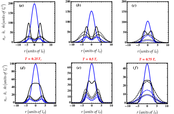
Figure 1: (Color online) Top row: density profiles of an immiscible mixture of ⁸⁷Rb (blue) and ¹³³Cs (black) atoms at different temperatures for $\Delta=0.9$. Solid lines: condensed density. Dashed lines: thermal cloud density. Dotted lines: anomalous density. The thermal cloud and the anomalous densities have been amplified by 10 times for clarity. Bottom row: same as top panels but for a miscible mixture for $\Delta=2.5$.

Figure 1 clearly shows that at low temperature, the Rb has a higher peak density and narrower width while the Cs atoms are pushed towards the outer part forming a shell structure around the Rb BEC [see Fig.1 (a)]. Such a symmetrical demixed phase, can be understood from the fact that the Rb sustains an extra confinement from the Cs shell surrounding it, i.e. originating from the coupling term $g_{12}n_{3-j}$ in Eq.(8). For phase separation, the TF approximation becomes less satisfactory. In this case, the Rb is located at the phase boundary, such that the density distribution varies fast in space and the kinetic terms cannot be omitted Pu .

At $T=0.5\,T_{c}$, the two components start to overlap with each other and the overlap region is broadened with temperature [see Fig.1(b)]. At $T\geq 0.75\,T_{c}$ where the binary condensates survive with significant thermal clouds, the mixture becomes completely immiscible as is depicted in Fig.1 (c). This suppression of the phase separation which has been predicted also by the HFB-Popov theory Arko , can be attributed to the strong effects of thermal fluctuations. We observe from the same figure that the anomalous density is larger than the noncondensed density at low temperature, it reaches its maximum at intermediate temperatures, and vanishes near the transition similar to the case of a single component. Indeed, this behavior remains valid irrespective of the mixture whether miscible or immiscible. At higher temperature, both $\tilde{n}$ and $\tilde{m}$ have a Gaussian shape since the system becomes ultra-dilute Boudj2 .

Figure 1 (d) shows that at $T=0.25\,T_{c}$, both species overlap at the trap center. Remarkably, with an increase in temperature ($T=0.5\,T_{c}$), the mixture becomes partially immiscible [see Fig.1 (e)]. As we have foreseen above, this phase transition is most likely due to the inclusion of the anomalous correlation which has a significant effect at this range of temperature. At $T\geq 0.75\,T_{c}$, the mixture restores its miscibility due to the weakness of $\tilde{m}$ [see Fig.1 (f)].

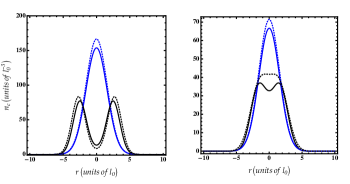
Figure 2: (Color online) Condensed density for $\Delta=0.9$ (left) and $\Delta=2.5$ (right) at $T=0.5\,T_{c}$. Solid lines: our predictions. Dotted lines: the results of the HFB-Popov theory. Parameters are the same as in Fig.1.

In Fig.2 we compare our results for the condensed density with the HFB-Popov calculations. As is clearly seen, the presence of the anomalous density leads to reduction of the condensed density and the degree of the overlap between the two condensates. This is owing to the mutual interaction between condensed atoms on the one hand and the condensed atoms and noncondensed atoms on the other.

III.2 Dynamics of spatial separation

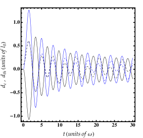
Figure 3: (Color online) Mean separation between the condensates (solid line) and thermal clouds (dotted lines) versus time in isotropic traps for $z_{0}/l_{0}=0.3$ and $\Delta=2.5$ at $T=0.5T_{c}$.

Figure 4: Mean separation between the condensates versus time in isotropic traps for ⁸⁷Rb atoms, with the scattering lengths are $a_{1}:a_{12}:a_{2}::1.03:1:0.97$, with the average of the three being 55 Å Hall . Solid line : our predictions. Dashed line: theoretical results of Sinatra . Plus: JILA experiment Hall . These data were taken after 22 ms after switching off the trapping potential.

Let us consider the evolution of dual condensates in the presence of their own thermal clouds and anomalous components confined in a spherically symmetric trap which at $t=0$ its centers for the first and second component are, respectively, displaced along the $z$-axis by distances $\pm z_{0}/2$. The separation is assumed to be small compared to the TF radii. The time dependence of the mean separation between the two condensates is given by

$$d_{c}(t)=\int d{\bf r}z\left[n_{c1}({\bf r},t)-n_{c2}({\bf r},t)\right],$$ (13)

while the mean separation between the two thermal clouds reads

$$d_{th}(t)=\int d{\bf r}z\left[\tilde{n}_{1}({\bf r},t)-\tilde{n}_{2}({\bf r},t)\right].$$ (14)

The numerical integration of our Eqs.(13) and (14) shows that at finite temperature, the relative motion of the centers-of-mass of the BECs and thermal clouds in a miscible mixture is strongly damped in particular at long time scales (see Fig.3). Such a damping, which has also been predicted by the ZNG theory Lee ; Lee1 , is caused by condensate-condensate, condensate-thermal, and thermal-thermal interactions. The intra- and inter-component anomalous pair correlations may play also a crucial role for the appearance of the aforementioned damping of oscillations especially at $T\approx 0.5\,T_{c}$. At fixed temperature, the damping of the oscillations of the mean separation between the condensates, and the thermal clouds becomes more and more strong for a large displacement, $z_{0}$, regime. One can expect that the same behavior persists in the immiscible mixture but with larger oscillation amplitudes.

To better understand the impact of the pair anomalous density on the damping mechanism, we compare our predictions for the relative motion of the centers-of-mass of the two BECs with the experimental measurements of Hall and the theoretical results of Sinatra based on the GP equation. As is clearly visible from Fig.4, the curves of our TDHFB model improve the theoretical result of Ref. Sinatra especially at large time scale. This correction makes our theory in good agreement with the JILA experiment Hall . The difference between the two models may be justified in terms of the significant contribution of the anomalous density which causes a huge loss of atoms during the oscillation even at zero temperature.

IV Homogeneous Bose-Bose mixture

In this section we analyze the elementary excitations in a homogeneous mixed Bose gas, where $V_{j}(r)=0$ using the generalized RPA Boudj1 ; Giorg ; Xia . This latter consists of imposing small fluctuations of the condensates, the noncondensates, and the anomalous components, respectively, as: $\Phi_{j}=\sqrt{n_{cj}}+\delta\Phi_{j}$, $\tilde{n}_{j}=\tilde{n}_{j}+\delta\tilde{n}_{j}$, and $\tilde{m}_{j}=\tilde{m}_{j}+\delta\tilde{m}_{j}$, where $\delta\Phi_{j}\ll\sqrt{n_{cj}}$, $\delta\tilde{n}_{j}\ll\tilde{n}_{j}$, and $\delta\tilde{m}_{j}\ll\tilde{m}_{j}$. Thus, we obtain the TDHFB-RPA equations

$$i\hbar\delta\dot{\Phi}_{j} =\left[h_{j}^{sp}+2\bar{g}_{j}n_{cj}+2g_{j}\tilde{n}_{j}+g_{12}n_{3-j}\right]\delta\Phi_{j}$$ (15)

$$+\bar{g}_{j}n_{cj}\delta\Phi_{j}^{*}+2g_{j}\sqrt{n_{cj}}\delta\tilde{n}_{j}+g_{12}\sqrt{n_{c{3-j}}}\delta\tilde{n}_{3-j}$$

$$+g_{12}\sqrt{n_{cj}n_{c{3-j}}}(\delta\Phi_{3-j}+\delta\Phi_{3-j}^{*}),$$

and

$$i\hbar\delta\dot{\tilde{m}}_{j} =4\left[h_{j}^{sp}+2g_{j}n_{j}+G_{j}(2\tilde{n}_{j}+1)+g_{12}n_{3-j}\right]\delta\tilde{m}_{j}$$ (16)

$$+8g_{j}\tilde{m}_{j}\left[\sqrt{n_{cj}}(\delta\Phi_{j}+\delta\Phi_{j}^{*})+\delta\tilde{n}_{j}+(G_{j}/g_{j})\delta\tilde{n}_{j}\right]$$

$$+g_{12}\tilde{m}_{j}\left[\sqrt{n_{c{3-j}}}(\delta\Phi_{3-j}+\delta\Phi_{3-j}^{*})+\delta\tilde{n}_{3-j}\right].$$

Here we recall that $\delta\tilde{n}_{j}$ and $\delta\tilde{m}_{j}$ are related with each other through (9). Remarkably, Eqs.(15) and (16) contain a class of terms beyond second order. They can be regarded as a natural extension of the HFB-RPA Xia theory developed for the single component BEC. If one neglects the anomalous density, the TDHFB-RPA equations reduce to the HFB-Popov-RPA equations.

Since we restrict ourselves to second order in the coupling constants, one must retain in Eqs.(15) and (16) only the terms which describe the coupling to the condensate and neglect all terms associated with fluctuations $\delta\tilde{n}$ and $\delta\tilde{m}$ Giorg . In fact, this assumption is relevant to ensure the gaplessness of the spectrum. Writting the field fluctuations associated to the condensate in the form $\delta\Phi_{j}({\bf r},t)=u_{jk}e^{i{\bf k\cdot r}-i\varepsilon_{k}t/\hbar}+v_{jk}e^{i{\bf k\cdot r}+i\varepsilon_{k}t/\hbar}$, we obtain the second order coupled TDHFB-de Gennes equations for the quasiparticle amplitudes $u_{kj}$ and $v_{kj}$ :

$$\begin{pmatrix}{\cal L}_{1}&{\cal M}_{1}&{\cal A}&{\cal A}\\ {\cal M}_{1}&{\cal L}_{1}&{\cal A}&{\cal A}\\ {\cal A}&{\cal A}&{\cal L}_{2}&{\cal M}_{2}\\ {\cal A}&{\cal A}&{\cal M}_{2}&{\cal L}_{2}\end{pmatrix}\begin{pmatrix}u_{1k}\\ v_{1k}\\ u_{2k}\\ v_{2k}\end{pmatrix}=\varepsilon_{k}\begin{pmatrix}u_{1k}\\ -v_{1k}\\ u_{2k}\\ -v_{2k}\end{pmatrix},$$ (17)

where $\int d{\bf r}[u_{j}^{2}({\bf r})-v_{j}^{2}({\bf r})]=1$, ${\cal L}_{j}=E_{k}+2\bar{g}_{j}n_{cj}+2g_{j}\tilde{n}_{j}+g_{12}n_{3-j}-\mu_{j}$, ${\cal M}_{j}=\bar{g}_{j}n_{cj}$, ${\cal A}=g_{12}\sqrt{n_{c1}n_{c2}}$, $\varepsilon_{k}$ is the Bogoliubov excitation energy and $E_{k}=\hbar^{2}k^{2}/2m$ is the kinetic energy which is the same for both species since we consider equal masses ($m_{1}=m_{2}=m$). For $g_{12}=0$, Eqs.(17) coincide with the finite temperature second-order equations obtained by Shi and Griffin using diagrammatic methods Griffin and with the finite temperature time-dependent mean-field scheme proposed by Giorgini Giorg . At zero temperature they correspond to the well-known second-order Beliaev’s results Beleav discussed in a single component Bose condensed gas over six decades ago, while at high temperature our second-order coupled TDHFB-de Gennes equations reproduce those derived by Fedichev and Shlyapnikov FedG employing Green’s function perturbation scheme.
The chemical potentials turn out to be given as

$$\mu_{j}=\bar{g}_{j}n_{cj}+2g_{j}\tilde{n}_{j}+g_{12}n_{3-j},$$ (18)

Inserting Eq.(18) into (17), one obtains the following Bogoliubov spectrum composed of two branches:

$$\varepsilon_{k+}=\sqrt{E_{k}^{2}+2E_{k}\mu_{+}}\,,\,\,\,\,\,\,\,\,\,\,\varepsilon_{k-}=\sqrt{E_{k}^{2}+2E_{k}\mu_{-}}\,,$$ (19)

where

$$\mu_{+,-}=\frac{\bar{g}_{1}n_{c1}}{2}f_{+,-}(\Delta,\alpha),$$ (20)

where $f_{+,-}(\Delta,\alpha)=1+\alpha\pm\sqrt{(1-\alpha)^{2}+4\Delta^{-1}\alpha}$ and $\alpha=\bar{g}_{2}n_{c2}/\bar{g}_{1}n_{c1}$.
In the limit $k\rightarrow 0$, we have $\varepsilon_{jk}=\hbar c_{j}k$ where $c_{j}=\sqrt{\bar{g}_{j}n_{cj}/m_{j}}$ is the sound velocity of a single condensate. The total dispersion is phonon-like in this limit

$$\varepsilon_{k(+,-)}=\hbar c_{+,-}k,$$ (21)

where the sound velocities $c_{+,-}$ are

$$c_{+,-}^{2}=\frac{1}{2}\left[c_{1}^{2}+c_{2}^{2}\pm\sqrt{\left(c_{1}^{2}-c_{2}^{2}\right)^{2}+4\Delta^{-1}c_{1}^{2}c_{2}^{2}}\right].$$ (22)

For $g_{12}^{2}>\bar{g}_{1}\,\bar{g}_{2}$, the spectrum (19) becomes unstable and thus, the two condensates spatially separate. We can see that the sound velocity $c_{+,-}\rightarrow 0$ as $T\rightarrow T_{c}$ since $n_{cj}=\tilde{m}_{j}=0$ near the transition, which means that the phonons in the TDHFB theory are the soft modes of the Bose-condensed mixture.

IV.1 Quantum and thermal fluctuations

A straightforward calculation using Eq.(9) permits us to rewrite the normal and anomalous densities in terms of $\sqrt{I_{k}}$ Boudj ; Boudj4

$$\tilde{n}_{j}=\frac{1}{2}\int\frac{d\bf k}{(2\pi)^{3}}\left[\frac{E_{k}+\mu_{+,-}}{\varepsilon_{k(+,-)}}\sqrt{I_{kj}}-1\right],$$ (23)

and

$$\tilde{m}_{j}=-\frac{1}{2}\int\frac{d\bf k}{(2\pi)^{3}}\frac{\mu_{+,-}}{\varepsilon_{k(+,-)}}\sqrt{I_{kj}}.$$ (24)

At $T=0$, the total depletion $\tilde{n}=\tilde{n}_{1}+\tilde{n}_{2}$ can be calculated via the integral (23)

$$\tilde{n}=\frac{1}{6\sqrt{2}\pi^{2}}\left(\frac{1}{\xi_{+}^{3}}+\frac{1}{\xi_{-}^{3}}\right),$$ (25)

where $\xi_{+,-}=\hbar/\sqrt{m\mu_{+,-}}$.
As remarked in integral (24), dimensional analysis suggests that we face the ultraviolet divergences in the expression of $\tilde{m}$ as anticipated above. This problem can be cured by means of the dimensional regularization Boudj ; Zin ; Klein ; Anders which follows from perturbation theory of scattering. It gives asymptotically exact results at weak interactions (for more details, see Appendix A of Boudj ). This yields for the total anomalous density $\tilde{m}=\tilde{m}_{1}+\tilde{m}_{2}$:

$$\tilde{m}=\frac{1}{2\sqrt{2}\pi^{2}}\left(\frac{1}{\xi_{+}^{3}}+\frac{1}{\xi_{-}^{3}}\right).$$ (26)

Importantly, the above expressions of the noncondensed and anomalous densities are proportional to $g_{j}^{2}$ and $g_{12}^{2}$. For $g_{12}=0$, Eqs.(25) and (26) recover those obtained by the second-order Beliaev theory Beleav and the perturbative time-dependent mean-field scheme Giorg .

From now onward, we assume that $\tilde{m}/n_{c}\ll 1$, this condition is valid at low temperature and necessary for the diluteness of the system Yuk ; Boudj2015 . Therefore, the condensate depletion (25) reduces to

$$\tilde{n}=\frac{1}{2\sqrt{2}}\tilde{n}_{1}^{0}\left[f_{+}^{3/2}(\Delta,\alpha)+f_{-}^{3/2}(\Delta,\alpha)\right],$$ (27)

where $\tilde{n}_{1}^{0}=(8/3)n_{c1}\sqrt{n_{c1}a_{1}^{3}/\pi}$ is the single condensate depletion (type-1). The depletion (27) is formally similar to that obtained by Tommasini et al. Tom using the Bogoliubov theory, with only $n_{cj}$ appearing as a corrected parameter instead of the total density $n_{j}$. At $T=0$ and for fixed density $\tilde{n}_{1}^{0}$, the noncondensed fraction is proportional to $\Delta$ and $\alpha$ signaling that the number of excited atoms increases with $\Delta$ and $\alpha$ as is displayed in Fig.5.
The anomalous density of the mixture (26) simplifies

$$\tilde{m}=\frac{1}{2\sqrt{2}}\tilde{m}_{1}^{0}\left[f_{+}^{3/2}(\Delta,\alpha)+f_{-}^{3/2}(\Delta,\alpha)\right],$$ (28)

where $\tilde{m}_{1}^{0}=8n_{c1}\sqrt{n_{c1}a_{1}^{3}/\pi}$ is the anomalous density of a single component. To the best of our knowledge, Eq.(28) has never been derived in the literature. It shows that $\tilde{m}$ is larger than $\tilde{n}$ similarly to the case of a single component. This indicates that the anomalous density is significant even at zero temperature in Bose-Bose mixtures. We see also that $\tilde{m}$ is increasing with $(n_{c1}a^{3})^{1/2}$, $\Delta$ and $\alpha$. If the interspecies and intraspecies interactions were strong enough, the pair anomalous density becomes important results in a large fraction of the total atoms would occupy the excited states.

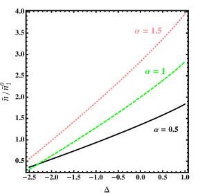
Figure 5: (Color online) Condensed depletion from Eq.(27) as a function of $\Delta$ for different values $\alpha$.

At temperatures $T\ll g_{1}n_{c1}$, the main contribution to integrals (23) and (24) comes from the long-wavelength region where the spectrum takes the form (21). Then the use of the integral $\int_{0}^{\infty}{x^{2j-1}\left[\coth(\alpha x)-1\right]dx}=\pi^{2j}|B_{2j}|/2j\alpha^{2j}$ Yuk , where $B_{2j}$ are the Bernoulli number, allows us to obtain the following expressions for the thermal contribution of the noncondensed and anomalous densities:

$$\tilde{n}_{th} =|\tilde{m}_{th}|=\frac{2\sqrt{2}}{3}n_{c1}\sqrt{\frac{n_{c1}a^{3}}{\pi}}\left(\frac{\pi T}{n_{c1}g_{1}}\right)^{2}$$ (29)

$$\times\left[f_{+}^{-1/2}(\Delta,\alpha)+f_{-}^{-1/2}(\Delta,\alpha)\right].$$

Equation (29) shows clearly that $\tilde{n}$ and $\tilde{m}$ are of the same order of magnitude at low temperature and only their signs are opposite. A comparaison between Eqs.(27), (28) and (29) shows that at $T\ll gn_{c}$, thermal fluctuations are smaller than the quantum fluctuations.

Let us now discuss some relevant cases predicted by Eqs.(27) and (28), for a balanced mixture where $n_{1}=n_{2}=n$, and $g_{1}=g_{2}=g_{12}$. Hence, the noncondensed and the anomalous densities reduce respectively to $\tilde{n}=(4/\sqrt{2})\,\tilde{n}^{0}$ and $\tilde{m}=(4/\sqrt{2})\,\tilde{m}^{0}$, whereas at low temperature, the thermal depletion and the anomalous density turn out to be given as $\tilde{n}_{th}=\tilde{m}_{th}=(2/3)n_{c1}\sqrt{n_{c1}a_{1}^{3}/\pi}\left(\pi T/n_{c1}g_{1}\right)^{2}$. Near the phase separation where $g_{12}^{2}\rightarrow\bar{g}_{1}\bar{g}_{2}$, the condensate depletion and the anomalous density become, respectively $\tilde{n}=(1+\alpha)^{3/2}\tilde{n}_{1}^{0}$ and $\tilde{m}=(1+\alpha)^{3/2}\tilde{m}_{1}^{0}$. At low temperature, the lower branch has the free-particle dispersion law: $\varepsilon_{k-}=E_{k}$ CFetter while the upper branch is phonon-like $\varepsilon_{k+}=\hbar c_{1}(1+\alpha)^{1/2}k$. Therefore, the thermal depletion has a distinct temperature dependence as

$$\tilde{n}_{th} =\frac{2}{3}n_{c1}\sqrt{\frac{n_{c1}a_{1}^{3}}{\pi}}(1+\alpha)^{-1/2}\left(\frac{\pi T}{n_{c1}g_{1}}\right)^{2}$$ (30)

$$+\left(\frac{mT}{2\pi\hbar^{2}}\right)^{3/2}\zeta(3/2),$$

where $\zeta(3/2)$ is the Riemann Zeta function. The second term in (30) is the density of noncondensed atoms in a noninteracting gas. This reveals that the component associated with lower branch becomes ultradilute. Notice that a similar temperature dependence distinction was obtained earlier by Colson and Fetter CFetter for ⁴He-⁶He mixture. Such a distinction in the temperature dependence cannot occur in $\tilde{m}_{th}$ where the term $\propto T^{3/2}$ is absent since the anomalous density itself does not exist in an ideal gas Boudj ; Griffin .

IV.2 Thermodynamics

Corrections to the EoS of the mixture due to quantum and thermal fluctuations can be derived from Eq.(18). Combining Eqs.(27), (28) and (29) gives

$$\delta\mu =\frac{\mu_{1}^{0}}{2\sqrt{2}}\bigg{\{}\left[f_{+}^{3/2}(\Delta,\alpha)+f_{-}^{3/2}(\Delta,\alpha)\right]$$ (31)

$$+\frac{1}{2}\left[f_{+}^{-1/2}(\Delta,\alpha)+f_{-}^{-1/2}(\Delta,\alpha)\right]\left(\frac{\pi T}{n_{c1}g_{1}}\right)^{2}\bigg{\}},$$

where $\mu_{1}^{0}=(32/3)g_{1}n_{c1}\sqrt{n_{c1}a_{1}^{3}/\pi}$ is the zero temperature chemical potential of a single condensate. At zero temperature and for $g_{12}=0$, Eq.(31) reduces to the seminal Lee-Huang-Yang (LHY) corrected EoS LHY for one component BEC.

At finite temperature, the grand-canonical ground state energy can be calculated using the thermodynamic relation $E=E_{0}+\delta E=-T^{2}\left(\frac{\partial}{\partial T}\frac{F}{T}\right)|_{V,\mu}$ where the free energy is given by $F=E+T\sum_{\bf k}\ln[1-\exp(-\varepsilon_{k(+,-)}/T)]$, and $E_{0}=(g_{j}/2)\sum_{j}(n_{cj}^{2}+4n_{cj}\tilde{n}_{j}+2\tilde{n}_{j}^{2}+|\tilde{m}_{j}|^{2}+2n_{cj}\tilde{m}_{j})+g_{12}n_{1}n_{2}$. When $\tilde{m}_{j}/n_{cj}\ll 1$ and $\tilde{n}_{j}/n_{cj}\ll 1$, one has $E_{0}=(g_{j}/2)\sum_{j}n_{cj}^{2}+g_{12}n_{c1}n_{c2}$. The shift to the ground state energy due to quantum and thermal fluctuations is defined as

$$\delta E =\frac{1}{2}\sum_{j}\bigg{[}\sum_{k}\left[\varepsilon_{k(+,-)}-(E_{k}+\mu_{+,-})\right]$$ (32)

$$+\sum_{k}\varepsilon_{k(+,-)}\left(\sqrt{I_{kj}}-1\right)\bigg{]}.$$

The first term on the r.h.s of (32) which represents the energy corrections due to quantum fluctuations is ultraviolet divergent. To circumvent such a divergency, we will use the standard dimensional regularization. The second term accounts for the thermal fluctuation contributions to the energy. The main contribution to it comes from the phonon region. After some algebra, we obtain

$$\delta E =\frac{1}{4\sqrt{2}}E_{1}^{0}\bigg{\{}\left[f_{+}^{5/2}(\Delta,\alpha)+f_{-}^{5/2}(\Delta,\alpha)\right]$$ (33)

$$+\frac{1}{2\sqrt{2}}\left[f_{+}^{-3/2}(\Delta,\alpha)+f_{-}^{-3/2}(\Delta,\alpha)\right]\left(\frac{\pi T}{n_{c1}g_{1}}\right)^{4}\bigg{\}},$$

where $E_{1}^{0}/V=(64/15)g_{1}n_{c1}^{2}\sqrt{n_{c1}a_{1}^{3}/\pi}$ is the zero-temperature single condensate ground state energy which can be obtained also by integrating the chemical potential with respect to the density. The same result could be obtained within the renormalization of coupling constants which consists of adding $g_{j}^{2}\int d{\bf k}/E_{k}$ and $g_{12}^{2}\int d{\bf k}/E_{k}$ Larsen ; Petrov to the r.h.s of Eq.(32).

In the case $g_{12}=0$, we read off from (33) that $\delta E$ reduces to the ground-state energy of a single Bose gas. At $T=0$ and for $n_{c}=n$, $\delta E$ becomes identical to the Larsan’s formula Larsen . Equation (33) is a finite-temperature extension of that recently obtained by Cappellaro et al. Capp for a balanced mixture using the functional integration formalism within a regularization of divergent Gaussian fluctuations. Indeed, the resulting ground-state energy is appealing since it furnishes an extra repulsive term proportional to $n_{c}^{5/2}+n_{c}^{-3/2}T^{4}$ balancing the attractive mean-field term, allowing quantum and thermal fluctuations to stabilize mixture droplets at finite temperature. Quantum stabilization and the related droplet nucleation was proposed in Bose-Bose mixtures with Petrov ; PetAst ; Cab ; Sem and without Rabi coupling Capp as well as applied on dipolar condensates Pfau ; Wach ; Bess ; Chom . The finite-temperature generalization of these LHY corrections to the case of a dipolar Bose gas has been also analyzed in our recent work BoudjDp .

V Conclusion and outlook

In this paper we have systematically studied effects of quantum and thermal fluctuations on the dynamics and the collective excitations of a two-component Bose gas utilizing the TDHFB theory. We revealed that our approach is able to capture the qualitative evolution of two-component BECs at finite temperature. The impact of the anomalous fluctuations on the miscibility criterion for the mixture was discussed.

Within an appropriate numerical method, we elucidated the behavior of the condensed, the noncondensed and the anomalous densities in terms of temperature for both miscible and immiscible mixtures under spherical harmonic confinement. We demonstrated in particular that the mixture undergoes a transition from miscible to immiscible regime owing to the predominant contribution of anomalous fluctuations notably at $T\simeq 0.5T_{c}$. We found that such fluctuations are also the agent responsible for the strong damping of the relative motion of the centers-of-mass of the condensed and thermal components. At zero temperature, the TDHFB results correct the existing theoretical models, making the theory in good agreement with JILA experiment Hall .

We linearized our TDHFB equations using the RPA for a weakly interacting uniform Bose-Bose mixture. This method is a finite-temperature extension of the famous second-order Beliaev approximation Beleav . The TDHFB-RPA theory provides us with analytical machinery powerful enough to calculate quantum and thermal fluctuation corrections to the excitations, the sound velocity, the EoS and the ground-state energy. We compared the theory with previous theoretical treatments and excellent agreement has been found in the limit $\tilde{m}/n_{c}\ll 1$. One should stress that the results of our TDHFB-RPA technique can be generalized to the case of a harmonically trapped mixture using the local density approximation.

The findings of this work are appealing for investigating the properties of mixture droplets at finite temperature. An important topic for future work is to look at how thermal fluctuations manifest themselves in dipolar Bose-Bose mixtures.

VI Acknowledgements

We are indebted to Eugene Zaremba and Hui Hu for stimulating discussions.

References

- (1) C. J. Myatt, E. A. Burt, R. W. Ghrist, E. A. Cornell, and C. E. Wieman, Phys. Rev. Lett.78, 586 (1997).
- (2) D. S. Hall, M. R. Matthews, J. R. Ensher, C. E. Wieman, and E. A. Cornell, Phys. Rev. Lett. 81, 1539 (1998).
- (3) P. Maddaloni, M. Modugno, C. Fort, F. Minardi, and M. Inguscio, Phys. Rev. Lett. 85, 2413 (2000).
- (4) C. R. Cabrera, L. Tanzi, J. Sanz, B. Naylor, P. Thomas, P. Cheiney, L. Tarruell, Science 359, 301 (2018); P. Cheiney, C. R. Cabrera, J. Sanz, B. Naylor, L. Tanzi, and L. Tarruell; inarXiv: 1710.11079v1 (2017).
- (5) G. Semeghini, G. Ferioli, L. Masi, C. Mazzinghi, L. Wolswijk, F.Minardi, M. Modugno, G. Modugno, M. Inguscio, and M. Fattori, arXiv:1710.10890v1 (2017).
- (6) S. B. Papp, J. M. Pino, and C. E.Wieman, Phys. Rev. Lett. 101, 040402 (2008).
- (7) S. Sugawa, R. Yamazaki, S. Taie, and Y. Takahashi, Phys. Rev. A 84, 011610 (2011).
- (8) G. Modugno, M. Modugno, F. Riboli, G. Roati, and M. Inguscio, Phys. Rev. Lett. 89, 190404 (2002); G. Thalhammer, G. Barontini, L. De Sarlo, J. Catani, F.Minardi, and M. Inguscio, ibid. 100, 210402 (2008).
- (9) D. J. McCarron, H.W. Cho, D. L. Jenkin, M. P. Köppinger, and S. L. Cornish, Phys. Rev. A 84, 011603 (2011).
- (10) A. D. Lercher, T. Takekoshi, M. Debatin, B. Schuster, R.Rameshan, F. Ferlaino, R. Grimm, and H.-C. Nägerl, Eur. Phys. J. D 65, 3 (2011).
- (11) B. Pasquiou, A. Bayerle, S. M. Tzanova, S. Stellmer, J. Szczepkowski, M. Parigger, R. Grimm, and F. Schreck, Phys. Rev. A 88, 023601 (2013).
- (12) L. Wacker, N. B. Jorgensen, D. Birkmose, R. Horchani, W.Ertmer, C. Klempt, N. Winter, J. Sherson, and J. J. Arlt, Phys. Rev. A 92, 053602 (2015).
- (13) F. Wang, X. Li, D. Xiong, and D. Wang, J. Phys. B 49, 015302 (2016).
- (14) I. Ferrier-Barbut, M. Delehaye, S. Laurent, A. T. Grier, M. Pierce, B. S. Rem, F. Chevy, and C. Salomon, Science 345, 1035 (2014).
- (15) S. Tojo, Y. Taguchi, Y. Masuyama, T. Hayashi, H. Saito, and T. Hirano, Phys. Rev. A 82, 033609 (2010).
- (16) E. Nicklas, H. Strobel, T. Zibold, C. Gross, B. A. Mal- omed, P. G. Kevrekidis, and M. K. Oberthaler, Phys. Rev. Lett. 107, 193001 (2011).
- (17) G. Barontini, C. Weber, F. Rabatti, J. Catani, G. Thalhammer, M. Inguscio, and F. Minardi, Phys. Rev. Lett. 103, 043201 (2009).
- (18) P. K. Molony, P. D. Gregory, Z. Ji, B. Lu, M. P. Köppinger, C. R. Le Sueur, C. L. Blackley, J. M. Hutson, and S. L. Cornish, Phys. Rev. Lett. 113, 255301 (2014).
- (19) Tin-Lun Ho and V. B. Shenoy, Phys. Rev. Lett. 77, 3276 (1996).
- (20) H. Pu and N. P. Bigelow, Phys. Rev. Lett. 80, 1130 (1998).
- (21) E. Timmermans, Phys. Rev. Lett. 81, 5718 (1998).
- (22) B. D. Esry, C. H. Greene, J. P. Burke, and J. L. Bohn, Phys. Rev. Lett. 78, 3594 (1997).
- (23) B. D. Esry and C. H. Greene, Phys. Rev. A 59, 1457 (1997).
- (24) M. Trippenbach, K. Goŕal, K. Rzaewski, B. Malomed, Y. B. Band, J. Phys. B 33, 4017 (2000).
- (25) F. Riboli and M. Modugno, Phys. Rev. A 65, 063614 (2002).
- (26) D. M. Jezek and P. Capuzzi, Phys. Rev. A 66, 015602 (2002).
- (27) A. A. Svidzinsky and S. T. Chui, Phys. Rev. A 67, 053608 (2003).
- (28) A. Sinatra, P. O. Fedichev, Y. Castin, J. Dalibard, and G. V. Shlyapnikov, Phys. Rev. Lett. 82, 251 (1999).
- (29) K. Kasamatsu, M. Tsubota, and M. Ueda, Phys. Rev. A 69, 043621 (2004).
- (30) D. M. Larsen, Ann. Phys. (N.Y.) 24, 89 (1963).
- (31) W. H. Bassichis, Phys. Rev. A 134, 543 (1964).
- (32) Y. A. Nepomnyashchii, Y. A. Nepomnnyashchii, Zh. Eksp. Teor. Fiz. 70, 1070 (1976) [Sov. Phys. - JETP 43, 559 (1976)]; Teor. Mat. Fiz. 20, 399 (1974).
- (33) A. S. Sorensen, Phys. Rev. A 65, 043610 (2002).
- (34) P.Tommasini, E. J. V. de Passos, A. F. R. de T. Piza, and M. S. Hussein, Phys. Rev. A 67, 023619 (2003).
- (35) W. B. Colson and A. L. Fetter, J. Low. Temp. Phys. 33, 231 (1978).
- (36) B. V. Schaeybroeck, Physica A 392, 3806 (2013).
- (37) C.-C. Chien, F. Cooper, and E. Timmermans, Phys. Rev. A 86, 023634 (2012).
- (38) H. Shi, W.-M. Zheng, and S.-T. Chui, Phys. Rev. A 61, 063613 (2000).
- (39) Arko Roy and D. Angom, Phys. Rev. A 92, 011601(R) (2015).
- (40) M. J. Edmonds, K. L. Lee, and N. P. Proukakis, Phys. Rev. A 91, 011602 (2015); 92, 063607 (2015).
- (41) K-L. Lee, N. B. Jorgensen, I-K. Liu, L. Wacker, J. Arlt, and N. P. Proukakis, Phys. Rev. A 94, 013602 (2016).
- (42) K-L. Lee and N. P. Proukakis J. Phys. B: At. Mol. Opt. Phys. 49, 214003 (2016).
- (43) Xiao-Long Chen, Xia-Ji Liu, and Hui Hu, Phys. Rev. A 96, 013625 (2017).
- (44) A. Boudjemâa, Degenerate Bose Gas at Finite Temperatures, LAP LAMBERT Academic Publishing (2017).
- (45) A. Boudjemâa and M. Benarous, Eur. Phys. J. D 59, 427 (2010) .
- (46) A. Boudjemâa and M. Benarous, Phys. Rev. A 84, 043633 (2011).
- (47) A. Boudjemâa, Phys. Rev. A 86, 043608 (2012).
- (48) A. Boudjemâa, Phys. Rev. A 88, 023619 (2013).
- (49) A. Boudjemâa, Phys. Rev. A 90, 013628 (2014).
- (50) A. Boudjemâa, J. Phys. A: Math. Theor. 48 045002 (2015).
- (51) A. Boudjemâa, Phys. Rev. A 91, 063633 (2015).
- (52) A. Boudjemâa, Commun. Nonlinear Sci. Numer. Simul. 33, 85 (2016).
- (53) A. Boudjemâa, Commun. Nonlinear Sci. Numer. Simul. 48, 376 (2017).
- (54) A. Boudjemâa, Phys. Rev. A 94, 053629 (2016).
- (55) A. Boudjemâa, and Nadia Guebli, J. Phys. A: Math. Theor. 50, 425004 (2017).
- (56) A. Griffin and H. Shi, Phys. Rep. 304, 1 (1998).
- (57) D. A. W. Hutchinson, R. J. Dodd, K. Burnett, S. A. Morgan, M. Rush, E. Zaremba, N. P. Proukakis, M. Edwards, and C. W. Clark, J. Phys. B 33, 3825 (2000).
- (58) V. I. Yukalov, Ann. Phys. 323, 461 (2008); Phys. Part. Nucl. 42, 460 (2011).
- (59) S. Giorgini, Phys. Rev. A 57, 2949 (1998); Phys. Rev. A 61, 063615 (2000).
- (60) H. Buljan, M. Segev, and A. Vardi, Phys. Rev. Lett. 95, 180401 (2005).
- (61) S. T. Beliaev, Sov. Phys. JETP 7, 289 (1958).
- (62) A. Boudjemâa, J. Phys. B: At. Mol. Opt. Phys. 48, 035302 (2015).
- (63) R. Balian and M. Vénéroni, Ann. Phys. (NY) 187, 29 (1988); 195, 324 (1989); 362, 838 (2015).
- (64) M. Benarous and H. Flocard, Ann. of Phys. 273, 242, (1999); M. Benarous, ibid. 264, 1 (2005).
- (65) C. Martin, Phys. Rev. D 52, 7121 (1995).
- (66) N. M. Hugenholtz and D. Pines, Phys. Rev. 116, 489 (1959).
- (67) A. A. Nepomnyashchy and Yu. A. Nepomnyashchy, JETP Lett. 21, 1 (1975); J. Exp. Theor. Phys. 48, 493 (1978); Yu. A. Nepomnyashchy, ibid. 58, 722 (1983).
- (68) R.A. Duine and H.T.C. Stoof, J. Opt. B: Quantum Semiclass. Opt. 5, S212 (2003).
- (69) S. Ospelkaus, C. Ospelkaus, L. Humbert, K. Sengstock, and K. Bongs, Phys. Rev. Lett. 97, 120403 (2006).
- (70) M. Zaccanti, C. DErrico, F. Ferlaino, G. Roati, M. Inguscio, and G. Modugno, Phys. Rev. A 74, 041605 (2006).
- (71) Xia-Ji Liu, Hui Hu, A. Minguzzi, and M. P. Tosi, Phys. Rev. A 69, 043605 (2004).
- (72) P. O. Fedichev and G. V. Shlyapnikov, Phys. Rev. A 58, 3146 (1998).
- (73) I. M. Khalatnikov, Zh. Eksp: Teor. Fiz., 32, 653 (1957).
- (74) Zinn-Justin J, Quantum field Theory and Critical Phenomena (Oxford University Press, New York, 2002)
- (75) Kleinert H, Path Integrals, World Scientific, Singapore, (2004)
- (76) J. O. Andersen, Rev. Mod. Phys 76, 599 (2004).
- (77) T. D. Lee, K. Huang and C. N. Yang, Phys. Rev 106, 1135 (1957).
- (78) D. S. Petrov, Phys. Rev. Lett. 115, 155302 (2015).
- (79) A. Cappellaro, T. Macrí, G. F. Bertacco and L. Salasnich, Sci. Rep. 7, 13358 (2017).
- (80) D. S. Petrov and G. E. Astrakharchik, Phys. Rev. Lett. 117, 100401 (2016).
- (81) I. Ferrier-Barbut, H. Kadau, M.Schmitt, M. Wenzel, T. Pfau, Phys. Rev. Lett. 116, 215301, (2016).
- (82) F. Wächtler and L. Santos, Phys. Rev. A 93, 061603 (R) (2016).
- (83) R. N. Bisset R. M. Wilson D. Baillie and P. B. Blakie, Phys. Rev. A 94, 033619 (2016).
- (84) L. Chomaz, S. Baier, D. Petter, M. J. Mark, F. Wächtler, L. Santos and F. Ferlaino, Phys. Rev. X 6, 041039 (2016).
- (85) A. Boudjemâa, Annals of Physics. 381, 68 (2017).