Topological phase transiton of anisotropic XY model with Dzyaloshinskii-Moriya interaction

Abstract

Within the real space renormalization group we obtain the phase portrait of the anisotropic quantum XY model on square lattice in presence of Dzyaloshinskii-Moriya (DM) interaction. The model is characterized by two parameters, $\lambda$ corresponding to XY anisotropy, and $D$ corresponding to the strength of DM interaction. The flow portrait of the model is governed by two global Ising-Kitaev attractors at $(\lambda=\pm 1,D=0)$ and a repeller line, $\lambda=0$. Renormalization flow of concurrence suggests that the $\lambda=0$ line corresponds to a topological phase transition. The gap starts at zero on this repeller line corresponding to super-fluid phase of underlying bosons; and flows towards a finite value at the Ising-Kitaev points. At these two fixed points the spin fields become purely classical, and hence the resulting Ising degeneracy can be interpreted as topological degeneracy of dual degrees of freedom. The state of affairs at the Ising-Kitaev fixed point is consistent with the picture of a p-wave pairing of strength $\lambda$ of Jordan-Wigner fermions coupled with Chern-Simons gauge fields.

I introduction

The two-dimensional classical (vector) XY model is a paradigm for the celebrated Berezinskii-Kosterlitz-Thouless (BKT) transition upon which the phase coherence of an underlying super-fluid is lost by the proliferation of topological excitations known as vortices Berezinskii (1971); Kosterlitz and Thouless (1973); Fradkin (2013). Quantum version of this model was initially proposed by Matsubara and Matsuda as a lattice model to understand the liquid helium Matsubara and Matsuda (1956). Since then there has been tremendous studies of the the two-dimensional quantum XY (2DQXY) model. Berezinskii used the term ”anisotropic planar magnetic substances” to refer to the quantum XY model Berezinskii (1972). The isotropic limit of the XY model refers to the situation where $\sigma^{x}\sigma^{x}$ and $\sigma^{y}\sigma^{y}$ couplings have equal strength. This is the isotropic limit of the XY model. Oitma and Betts found that the ground state of this model has finite transverse magnetization Oitma and Betts (1978). The exact diagonalization study of Tang on the anti-ferromagnetic XY model found isotropic staggered magnetization in the XY plane Tang (1988). Drzewinsky and Sznajd used a block-spin renormalization group at finite temperatures to find a BKT transition temperature in this system Drzewinski and Sznajd (1989). The BKT transition for the 2DQXY was confirmed in quantum Monte Carlo studies Ding and Makivić (1990); Ding (1992); Ying et al. (1998); Harada and Kawashima (1998). The critical exponents extracted from the quantum Monte Carlo study of Ding and coworkers suggested that 2DQXY belongs to the same universality class as the classical (vector) XY model Ding (1992).

An equivalent way of thinking about 2DQXY model is in terms of hardcore bosons Carrasquilla and Rigol (2012). This bosonic language is particularly convenient for the study of super-fluid transition measured by super-fluid density, $\rho_{s}$, which in the spin language corresponds to spin-stiffness Sachdev (2011). In the bosonic language for a system with filling fraction $n$ at the classical level the zero temperature super-fluid-density is given by $\rho_{s}^{\rm cl}\propto n(1-n)$. Quantum fluctuations enhance the above stiffness by few percent Sandvik and Hamer (1999). The emerging picture is that the zero temperature phase of the isotropic 2DQXY is that of a super-fluid. Indeed in a remarkable paper a much stronger version of this for all spins and for all dimensions higher than one was proven by Kennedy, Lieb and Shastry Kennedy et al. (1988).

Extensions of the isotropic 2DQXY model are also very interesting. Dekeyser and coworkers employed the quantum renormalization group method to suggest that extending the 2DQXY by an $\sigma^{z}\sigma^{z}$ Ising term gives a very simple picture that the greater of Ising and XY exchange interaction dominates the low-energy phase Dekeyser et al. (1977). Such an Ising exchange is equivalent to interaction among bosons. Placing this model on triangular lattice Heidarian and Damle (2005) sets a very interesting competition between the Mott localization, geometric frustration and super-fluidity of hardcore bosons where a diagonal solid order emerges at strong interactions Melko et al. (2005) and remains stable for arbitrary large values of interaction Heidarian and Damle (2005). This can be a possible explanation for the super-solid phase of helium Kim and W (2004). Another possible extension is by plaquette interactions in presence of an external field where the four-site terms encourage valence bond solid Melko et al. (2004). Allowing for bond-disorder in the 2DQXY model enhances the amplitude of zero-point phase fluctuations giving rise to vanishing of the spin-stiffness which then turns the ground state into spin liquid Gawiec and Grempel (1996).

In addition to the above bosonic picture of the 2DQXY model and its extensions, there is also fermionic picture which is based on a Jordan-Wigner transformation. In this approach the spin system is mapped into a Chern-Simons (CS) theory coupled with spin-$1/2$ fermions Fradkin (1989); Lopez et al. (1994); Fradkin (2013). This mapping is quite general and applies to larger family of spin systems than the 2DQXY on any bipartite lattice Wang (1991). This approach is quite powerful, and is used to relate the $1/3$ magnetization plateau of the regime of XY anisotropy to a bosonic fractional Laughlin state with filling fraction $1/2$ Kumar et al. (2014).

In this paper we extend the anisotropic 2DQXY model by adding a Dzyaloshinskii-Moriya (DM) interaction of strength $D$. We consider a planar anisotropy $\lambda$ that makes the exchange in $x$ and $y$ directions different. On top of that we add a DM interaction between the planar components of the spin. We employ the block-spin renormalization group (BSRG) to study the phase transitions of this model. We construct a phase portrait of the model from our BSRG equations. We find that there are two global attractors that attract the flow to gapped states which correspond to Ising phases polarized along $x$ or $y$ directions Tang (1988). These two are separated by a gap-closing and hence should correspond to topologically non-trivial phases, similar to its one-dimensional counterpart Jafari (2017). We corroborate the topological nature of this quantum phase transition with the calculation of concurrence. The whole $\lambda=0$ line in the plane of $\lambda$ and $D$ will be a gapless repeller which is unstable with respect to smallest anisotropy $\lambda$ (irrespective of the sign of $\lambda$). This is reminiscent of the pairing instability in a gapless system of Jordan-Winger fermions Jafari (2017) which from the exact solution of the one-dimensional problem can be interpreted as the p-wave pairing interaction. Indeed such a p-wave pairing resulting from the anisotropy $\lambda$ can be obtained from the study of equivalent fermions coupled to Chern-Simons gauge fields on the honeycomb lattice Sedrakyan et al. (2017).

The paper is organized as follows. In Sec. II the XY model in the presence of DM interaction has been considered. The effective Hamiltonian of the system for the renormalized coupling constant and anisotropic parameters is obtained. In the Sec. III we present the details of the phase diagram. The discussions and results are presented in Sec. IV.

II Model and method

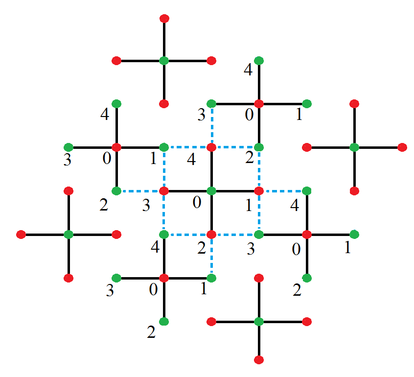
Figure 1: (Color online) The selected cluster in a square lattice where the dashed lines shows the block-block interactions.

The Hamiltonian of XY model on a 2D square lattice in the presence of DM interaction with N$\times$N sites can be written as,

$$H(J,\lambda,D) =$$

$$J\sum_{i=1}^{N}\sum_{j=1}^{N}[(1+\lambda)\left(\sigma_{i,j}^{x}\sigma_{i+1,j}^{x}+\sigma_{i,j}^{x}\sigma_{i,j+1}^{x}\right)$$

$$+(1-\lambda)(\sigma_{i,j}^{y}\sigma_{i+1,j}^{y}+\sigma_{i,j}^{y}\sigma_{i,j+1}^{y})$$

$$+D(\sigma_{i,j}^{x}\sigma_{i+1,j}^{y}-\sigma_{i,j}^{y}\sigma_{i+1,j}^{x})$$

$$+D(\sigma_{i,j}^{x}\sigma_{i,j+1}^{y}-\sigma_{i,j}^{y}\sigma_{i,j+1}^{x})]$$ (1)

where $J>0$ is the exchange coupling, $\lambda$ is anisotropy parameter, $D$ is the DM interaction term and $\sigma_{i}^{n}~{}(n=x,y,z)$ are Pauli matrices at site $i$. The basic idea of block-spin renormalization method is to partition the lattice into clusters. Then if the cluster allows for a Kramers doublet ground states, the fluctuations between such doublet can be captured with an effective (coarse grained) spin variable González et al. (2008); MARTÍN-DELGADO and SIERRA (1996).

II.1 Block spin RG equations

To study the ground state phases of the above Hamiltonian, we partition the square lattice into blocks of five sites as depicted in Fig. 1. Out of the five sites in the cluster, four are from one sub-lattice and one is from the other sub-lattice. For interactions involving the Ising term of the form $\sigma^{z}\sigma^{z}$ such a sub-lattice imbalance erroneously biases the ground state towards the wrong ground state total spin. This is due to Lieb-Mattis theorem for the Hubbard and Heisenberg family of models. However for XY family where the only conserved charge is $\zeta=\prod_{j}\sigma^{z}_{j}$ Jafari (2017) where $j$ runts over the whole lattice, this sub-lattice asymmetry does not destroy the doublet structure of the ground state and we still get a doublet of ground states each belonging to $\zeta=\pm 1$ sectors. The conserved charge $\zeta$ already breaks the $2^{5}$ dimensional Hilbert space into two sectors, each of dimension $16$. States in each sector are in one-to-one correspondence in the above two sectors. These two sectors are mapped to each other by replacing the role of $\uparrow$ and $\downarrow$ spins. The clusters in Fig. 1 have further four-fold rotational symmetry. This allows to use standard methods of group theory Dresselhaus et al. (2007) to further reduce the $16$ dimensional space corresponding to a given $\zeta$. The details of the straightforward but lengthily algebra is given in the appendix. The sector that contains the ground state is a $6\times 6$ dimensional space which can be diagonalized to give the set of eigenvalues depicted in Fig. 2 in the parameter space of $D,\lambda$.

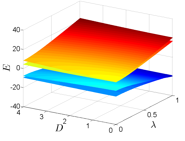
Figure 2: (Color online) (a) The bands plots of selected five-site cluster in terms of $\lambda$ and $J$ when $D=0$. (b) The plots of bands in nonzero DM interaction at $J=1$.

The ground state energy in both $\zeta=\pm 1$ sectors is

$$e_{0}=-2J\sqrt{5(1+D^{2})+5\lambda^{2}+\eta},$$ (2)

where

$$\eta=\sqrt{\lambda^{4}+34\lambda^{2}(1+D^{2})+(1+D^{2})^{2}}$$ (3)

and the ground state eigen-vector in the $\zeta=+1$ sector is,

$$|\phi_{+}\rangle= \gamma_{1}|\downarrow\downarrow\downarrow\downarrow\downarrow\rangle+\gamma_{2}|\uparrow\uparrow\uparrow\uparrow\downarrow\rangle+\gamma_{3}(|\uparrow\uparrow\uparrow\downarrow\uparrow\rangle+|\uparrow\uparrow\downarrow\uparrow\uparrow\rangle$$

$$+|\uparrow\downarrow\uparrow\uparrow\uparrow\rangle+|\downarrow\uparrow\uparrow\uparrow\uparrow\rangle)+\gamma_{4}(|\uparrow\downarrow\downarrow\downarrow\uparrow\rangle+|\downarrow\downarrow\downarrow\uparrow\uparrow\rangle$$

$$+|\downarrow\uparrow\downarrow\downarrow\uparrow\rangle+|\downarrow\downarrow\uparrow\downarrow\uparrow\rangle)+\frac{\sqrt{2}}{2}(|\uparrow\downarrow\downarrow\uparrow\downarrow\rangle+|\uparrow\uparrow\downarrow\downarrow\downarrow\rangle$$

$$+|\downarrow\downarrow\uparrow\uparrow\downarrow\rangle+|\downarrow\uparrow\uparrow\downarrow\downarrow\rangle+|\uparrow\downarrow\uparrow\downarrow\downarrow\rangle+|\downarrow\uparrow\downarrow\uparrow\downarrow\rangle).$$ (4)

The ground state in $\zeta=-1$ sector is simply obtained by the spin-flip transformation of the above ground state, $\uparrow\leftrightarrow\downarrow$.

$$|\phi_{-}\rangle= \gamma_{1}|\uparrow\uparrow\uparrow\uparrow\uparrow\rangle+\gamma_{2}|\downarrow\downarrow\downarrow\downarrow\uparrow\rangle+\gamma_{3}(|\downarrow\downarrow\downarrow\uparrow\downarrow\rangle+|\downarrow\downarrow\uparrow\downarrow\downarrow\rangle$$

$$+|\downarrow\uparrow\downarrow\downarrow\downarrow\rangle+|\uparrow\downarrow\downarrow\downarrow\downarrow\rangle)+\gamma_{4}(|\downarrow\uparrow\uparrow\uparrow\downarrow\rangle+|\uparrow\uparrow\uparrow\downarrow\downarrow\rangle$$

$$+|\uparrow\downarrow\uparrow\uparrow\downarrow\rangle+|\uparrow\uparrow\downarrow\uparrow\downarrow\rangle)+\frac{\sqrt{2}}{2}(|\downarrow\uparrow\uparrow\downarrow\uparrow\rangle+|\downarrow\downarrow\uparrow\uparrow\uparrow\rangle$$

$$+|\uparrow\uparrow\downarrow\downarrow\uparrow\rangle+|\uparrow\downarrow\downarrow\uparrow\uparrow\rangle+|\downarrow\uparrow\downarrow\uparrow\uparrow\rangle+|\uparrow\downarrow\uparrow\downarrow\uparrow\rangle)$$ (5)

where the coefficients are obtained as,

$$\gamma_{1}=\frac{6\sqrt{2}\lambda(1+iD)}{5(1+D^{2})+\lambda^{2}+\eta}$$

$$\gamma_{2}=\frac{\sqrt{2}(1+iD)(-1+\lambda^{2}-D^{2}+\eta)}{\lambda(5(1+D^{2})+\lambda^{2}+\eta)}$$

$$\gamma_{3}=\frac{(-1-5\lambda^{2}-D^{2}+\eta)\sqrt{5(1+D^{2})+5\lambda^{2}+\eta}}{4\sqrt{2}\lambda(-1-D^{2}+\lambda^{2})}$$

$$\gamma_{4}=-\frac{3i(-i+D)\sqrt{5(1+D^{2})+5\lambda^{2}+\eta}}{{5(1+D^{2})+\lambda^{2}+\eta}}.$$ (6)

As illustrated in Fig. 2 the presence of DM interaction will not generate any band crossing and the ground state remains stable with respect to change of anisotropy parameters and DM interactions. The relation between Hamiltonian (1) and the coarse-grained effective Hamiltonian is formally given as,

$$H^{\rm eff}=T^{\dagger}_{0}HT_{0},$$ (7)

where the projection operator $T_{0}$ basically assigns a new coarse grained spins $\Uparrow,\Downarrow$ to the two degenerate (Kramers double) ground states $|\phi_{+}\rangle$ and $|\phi_{-}\rangle$ in the $\zeta=\pm 1$ sectors:

$$T_{0}=|\phi_{+}\rangle\langle\Uparrow|+|\phi_{-}\rangle\langle\Downarrow|.$$ (8)

The Pauli matrix $\sigma^{z}_{j}$ can not change the charge $\zeta=\pm 1$ and therefore in the space composed of doublet of $|\phi_{\pm}\rangle$, the action of each $\sigma^{z}_{j}$ contributes to the formation of a coarse grained $\sigma^{\prime z}$ for the whole cluster. Similarly each $\sigma^{x(y)}_{j}$ flips one of the spins, thereby flipping the sign of $\zeta$ and can be interpreted as flipping the coarse grained spins $|\Uparrow\rangle$ and $|\Downarrow\rangle$ which can then be represented by $\sigma^{\prime x(y)}$ in the space of coarse grained spins. In this process some coefficients from the ground state wave function will be collected. For the coupling of neighboring coarse-grained spins one needs to collect interactions on the bonds connecting a cluster to its neighbors Jafari (2017). The effective Hamiltonian in the $n$’th step of the above process will be

$$H(J_{n},\lambda_{n},D_{n}) =$$

$$J_{n}\sum_{r=1}^{N/5}\sum_{s=1}^{N/5}[(1+\lambda_{n})(\sigma_{r,s}^{x}\sigma_{r+1,s}^{x}+\sigma_{r,s}^{x}\sigma_{r,s+1}^{x})$$

$$+(1-\lambda_{n})(\sigma_{r,s}^{y}\sigma_{r+1,s}^{y}+\sigma_{r,s}^{y}\sigma_{r,s+1}^{y})$$

$$+D_{n}(\sigma_{r,s}^{x}\sigma_{r+1,s}^{y}-\sigma_{r,s}^{y}\sigma_{r+1,s}^{x})$$

$$+D_{n}(\sigma_{r,s}^{x}\sigma_{r,s+1}^{y}-\sigma_{r,s}^{y}\sigma_{r,s+1}^{x})],$$ (9)

where the BSRG transformation connecting two consecutive steps becomes,

$$J_{n+1}=\frac{\alpha^{2}+\xi^{2}+\left(\alpha^{2}-\xi^{2}\right)\lambda_{n}}{2}J_{n}$$

$$\lambda_{n+1}=\frac{\alpha^{2}-\xi^{2}+\left(\alpha^{2}+\xi^{2}\right)\lambda_{n}}{\alpha^{2}+\xi^{2}+\left(\alpha^{2}-\xi^{2}\right)\lambda_{n}}$$

$$D_{n+1}=\frac{2\alpha\xi}{\alpha^{2}+\xi^{2}+\left(\alpha^{2}-\xi^{2}\right)\lambda_{n}}D_{n}.$$ (10)

The coefficients are given by,

$$\alpha=\frac{1}{\mathcal{N}^{2}} [\gamma_{1}\gamma_{3}^{*}+\gamma_{3}\gamma_{1}^{*}+\gamma_{2}\gamma_{4}^{*}+\gamma_{4}\gamma_{2}^{*}$$

$$\frac{3\sqrt{2}}{2}(\gamma_{3}+\gamma_{3}^{*}+\gamma_{4}+\gamma_{4}^{*})]$$

$$\xi=\frac{1}{\mathcal{N}^{2}} [\gamma_{1}\gamma_{3}^{*}+\gamma_{3}\gamma_{1}^{*}-\gamma_{2}\gamma_{4}^{*}-\gamma_{4}\gamma_{2}^{*}$$

$$\frac{3\sqrt{2}}{2}(-\gamma_{3}-\gamma_{3}^{*}+\gamma_{4}+\gamma_{4}^{*})]$$

with

$$\mathcal{N}=\sqrt{|\gamma_{1}|^{2}+|\gamma_{2}|^{2}+4|\gamma_{3}|^{2}+4|\gamma_{4}|^{2}+3}.$$

The $\gamma_{i}^{*}$ is the conjugate of $\gamma_{i}$ and $|\gamma_{i}|^{2}=\gamma_{i}\gamma_{i}^{*}$.

II.2 Entanglement analysis

Among various tools, entanglement is standard tool for the diagnosis of the phase transitions in general Amico et al. (2008); Kargarian et al. (2007, 2008); Langari (2004); Song et al. (2013, 2014); Ma et al. (2011); Liu et al. (2016) and change of topology Kitaev and Preskill (2006); Jiang et al. (2012); Cho and Kim (2017) in particular. Therefore let us use this tool in our five-site problem and to study its evolution under the RG transformations obtained above. Let us consider the entanglement between two spins in the corners of each blocks. For this purpose we first calculate the reduced density matrix between every two pairs of neighboring sites, namely, $\rho_{12}$, $\rho_{13}$, $\rho_{14}$, $\rho_{23}$, $\rho_{24}$ and $\rho_{34}$ which involves tracing out all the rest of degrees of freedom Bennett et al. (1996); Hill and Wootters (1997). To construct the $4\times 4$ matrix $\rho_{ij}$ ($i,j$ are site indices, not matrix indices) one first constructs the full density matrix,

$$\rho=|\psi_{0}\rangle\langle\psi_{0}|$$ (11)

where the $|\psi_{0}\rangle$ can be any of the Kramers doublet degenerate ground states $|\phi_{\pm}\rangle$ and then traces all sites except for sites $i,j$. We then form a matrix $\rho_{ij}\tilde{\rho}_{ij}$ where $\tilde{\rho}_{ij}=\left(\sigma^{y}_{i}\otimes\sigma^{y}_{j}\right)\rho^{*}_{ij}\left(\sigma^{y}_{i}\otimes\sigma^{y}_{j}\right)$ and number its four eigenvalues such that $\lambda_{ij,m},~{}(m=1,2,3,4)$ such that $\lambda_{ij,4}>\lambda_{ij,3}>\lambda_{ij,2}>\lambda_{ij,1}$. From these eigenvalues we then evaluate the bipartite concurrence defined by Hill and Wootters (1997),

$$C_{ij}=max\left(\sqrt{\lambda_{ij,4}}-\sqrt{\lambda_{ij,3}}-\sqrt{\lambda_{ij,2}}-\sqrt{\lambda_{ij,1}},~{}0\right).$$

Then we construct a geometric mean of the concurrence between the above 6 pairs of sites as Hill and Wootters (1997),

$$C_{g}=\sqrt[6]{C_{12}\times C_{13}\times C_{14}\times C_{23}\times C_{24}\times C_{34}}.$$ (12)

In the present case, by rotational symmetry all of the six density matrices are equal and given by

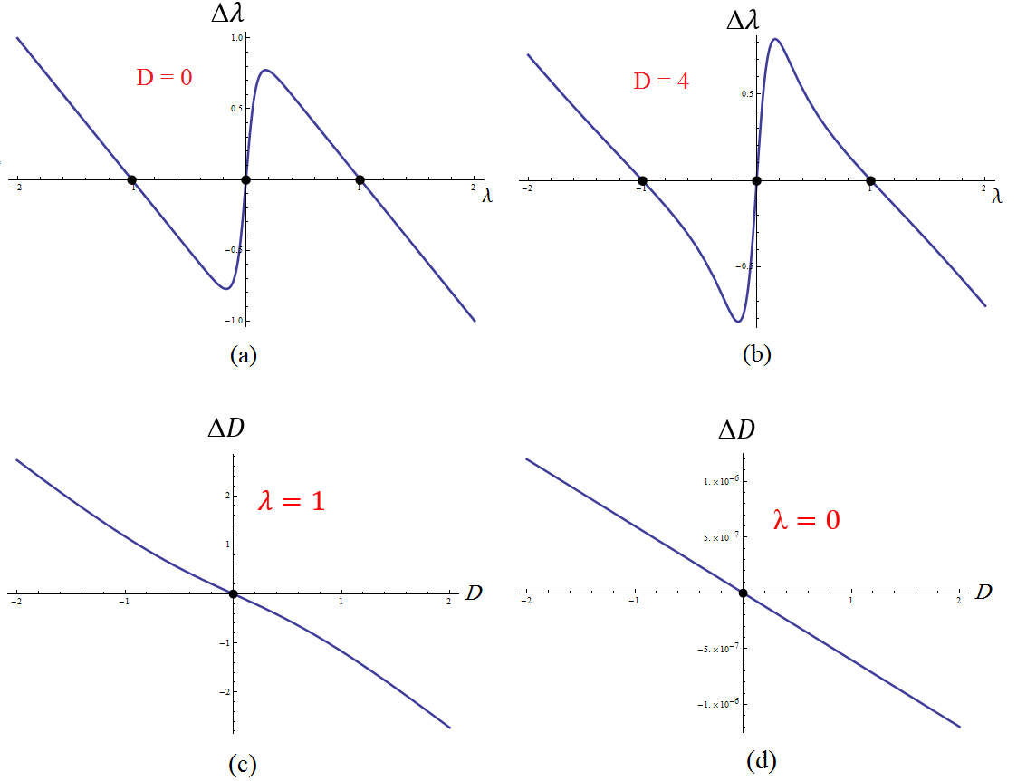
Figure 3: (Color online) Fixed points of the 2DQXY model with anisotropy ($\lambda$) and DM interaction ($D$). In top (bottom) row we have fixed $D$ ($\lambda$) to study flow of $\lambda$ ($D$). There are two attractors at $\lambda=\pm 1$ and a repulsive fixed point at $\lambda=0$. The DM interaction has only one attractor at $D=0$.

$$\rho_{12}=\rho_{23}=\rho_{34}= \rho_{13}=\rho_{14}=\rho_{24}=$$

$$=\frac{1}{\mathcal{N}^{2}}\left(\begin{matrix}\gamma_{1}\gamma_{1}^{*}+2\gamma_{4}\gamma_{4}^{*}+\frac{1}{2}&0&0&\frac{\sqrt{2}}{2}(\gamma_{1}+\gamma_{2}^{*})+2\gamma_{4}\gamma_{3}^{*}\\ 0&\gamma_{3}\gamma_{3}^{*}+\gamma_{4}\gamma_{4}^{*}+1&\gamma_{3}\gamma_{3}^{*}+\gamma_{4}\gamma_{4}^{*}+1&0\\ 0&\gamma_{3}\gamma_{3}^{*}+\gamma_{4}\gamma_{4}^{*}+1&\gamma_{3}\gamma_{3}^{*}+\gamma_{4}\gamma_{4}^{*}+1&0\\ \frac{\sqrt{2}}{2}(\gamma_{1}^{*}+\gamma_{2})+2\gamma_{4}^{*}\gamma_{3}&0&0&\gamma_{2}\gamma_{2}^{*}+2\gamma_{3}\gamma_{3}^{*}+\frac{1}{2}\\ \end{matrix}\right)$$ (13)

The above matrix gives,

$$C_{g}=\frac{\sqrt{\Gamma_{2}^{2}+2\Gamma_{1}\Gamma_{3}+\Gamma_{2}^{*2}+2\sqrt{\Lambda}\Re\Gamma_{2}}}{\sqrt{2}}-\frac{\sqrt{\Gamma_{2}^{2}+2\Gamma_{1}\Gamma_{3}+\Gamma_{2}^{*2}-2\sqrt{\Lambda}\Re\Gamma_{2}}}{\sqrt{2}}-2\sqrt{\Gamma_{4}}$$ (14)

where $\Lambda=\sqrt{\Gamma_{2}^{2}+4\Gamma_{1}\Gamma_{3}-2\Gamma_{2}\Gamma_{2}^{*}+\Gamma_{2}^{*2}}$, $\Gamma_{1}=\frac{1}{\mathcal{N}^{2}}\left(\gamma_{1}\gamma_{1}^{*}+2\gamma_{4}\gamma_{4}^{*}+\frac{1}{2}\right)$, $\Gamma_{2}=\frac{1}{\mathcal{N}^{2}}\left(\frac{\sqrt{2}}{2}(\gamma_{1}+\gamma_{2}^{*})+2\gamma_{4}\gamma_{3}^{*}\right)$, $\Gamma_{3}=\frac{1}{\mathcal{N}^{2}}\left(\gamma_{3}\gamma_{3}^{*}+\gamma_{4}\gamma_{4}^{*}+1\right)$ and $\Gamma_{4}=\frac{1}{\mathcal{N}^{2}}\left(\gamma_{2}\gamma_{2}^{*}+2\gamma_{3}\gamma_{3}^{*}+\frac{1}{2}\right)$. We will use the above formula in our analysis of the phase transitions of the 2DQXY with planar anisotropy $\lambda$ and DM interaction $D$.

III Phase diagram of the model

III.1 Analysis of the phase portrait

The standard method for analysis of the phase diagram of a model that depends on set of parameters ${\mathbf{R}}$ is to study $\Delta{\mathbf{R}}_{n}\equiv{\mathbf{R}}_{n+1}-{\mathbf{R}}_{n}$ and its dependence to the initial values ${\mathbf{R}}_{0}\equiv{\mathbf{R}}$ Strogatz (2014); Jafari (2017). In our problem the parameters are given by ${\mathbf{R}}=(\lambda,D)$. In Fig. 3 we have presented two such cuts. In the first row, for two fixed values of $D=0$ (left) and $D=4$ (right) we plot how $\Delta\lambda$ depends on the initial value $\lambda$. As can be seen there are two fixed points. Repulsive fixed point at $\lambda_{*}^{0}=0$ and two attractors at $\lambda_{*}^{\pm}=\pm 1$ Jafari (2017). These values do not change by replacing $D=0$ with $D=4$. In the second row of Fig. 3, for two fixed values of $\lambda=0$ and $\lambda=1$ we have plotted how $\Delta D$ depends on the initial value $D$. As can be seen, independent of value of $\lambda$, there is always an attractor at $D_{*}=0$: Slightly moving to the right (left) of $D_{*}=0$, gives a negative (positive) $\Delta D$ that returns $D$ to the attractor $D_{*}=0$. Therefore the coupling $D$ is irrelevant and any Hamiltonian of the form (1) with a non-zero $D$ in the long wave-length limit behaves similar to the $D_{*}=0$ and the DM interaction is renormalized away in the infrared limit.

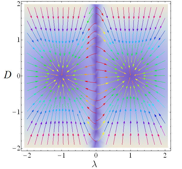
Figure 4: (Color online) Phase portrait of the 2DQXY model with anisotropy $\lambda$ and DM interaction $D$. Two global attractors at $(\lambda_{*}^{\pm},D_{*})=(\pm 1,0)$ along with repeller at infinity and a repulsive line $(\lambda_{*}^{0},D)$ for every $D$, completely characterize the above RG flow profile.

Let us put the above picture in a global perspective in a plane composed of $\lambda$ and $D$. In Fig. 4 we have provided a stream plot of the vectors $\Delta{\mathbf{R}}=(\Delta\lambda,\Delta D)$ as a function of the initial value ${\mathbf{R}}=(\lambda,D)$. As can be seen the fact that in Fig. 3 the fixed point at $\lambda_{*}^{\pm}$ does not depend on $D$ is reflected in Fig. 4 as the fact that the two attractors at $(\lambda_{*}^{\pm},D_{*})=(\pm 1,0)$ are globally attractive fixed points. However the fact that the repulsive fixed point $\lambda_{*}^{0}$ in Fig. 3 does not depend on $\lambda$ is reflected in Fig. 4 as a repulsive line. The symmetry of the above phase portrait under $\lambda\to-\lambda$ is the direct manifestation of the fact that Hamiltonian is invariant under $\sigma_{j}^{x}\to\sigma_{j}^{y}$, $\sigma_{j}^{y}\to-\sigma_{j}^{x}$ ($\pi/2$ rotation around $z$ axis), $D\to D$ and $\lambda\to-\lambda$.

III.2 Analysis of the gap

So far our phase portraits in Figs. 3 and 4 indicate the irrelevance of $D$ and a possible phase transition at $\lambda=0$ line. Let us see how does this manifest itself in the spectral gap. The gap between the ground state and the first excited state is given by,

$$E_{g}^{C} =$$ (15)

$$2J\left[\sqrt{5(1+D^{2})+5\lambda^{2}+\eta}-\sqrt{5(1+D^{2})+5\lambda^{2}-\eta}\right]$$

The effect of RG flow on this quantity when it is iterated up to large enough RG steps to ensure machine precision convergence is plotted in Fig. 5 for various values of the DM interaction $D$ indicated in the legend. In this figure we plot the gap at the 8-th RG step (converged within $10^{-5}$). As can be seen for every value of $D$, the point $\lambda_{*}^{0}=0$ is the only gapless point, and any non-zero value of $\lambda$, either positive or negative gives rise to a non-zero gap. The gap is normalized per lattice site, and the natural unit of the gap is $J$. The fact that for every value of $D$ we have a non-zero gap for $\lambda\neq 0$ agrees with the existence of a line of fixed points $\lambda=\lambda_{*}^{0}$ in the $(\lambda,D)$ plane of Fig. 4.

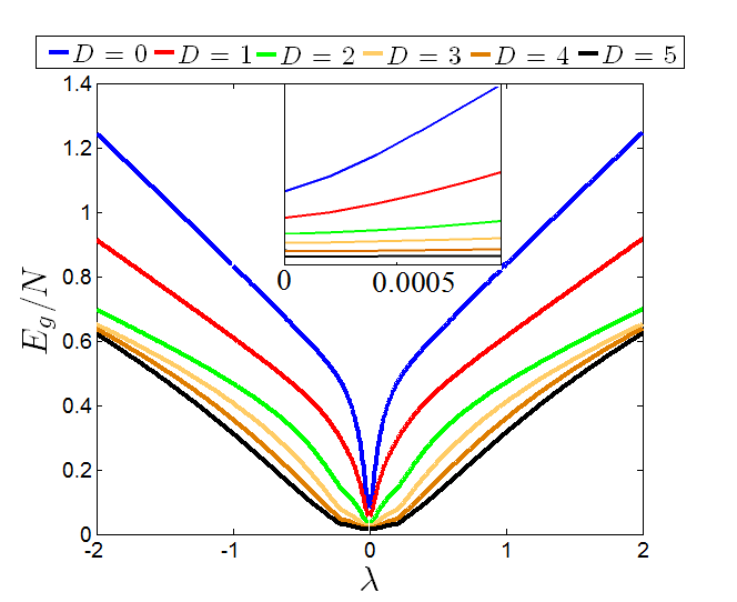
Figure 5: (Color online) Dependence of the gap on anisotropy $\lambda$ for various values of the DM interaction $D$ indicated in the legend.

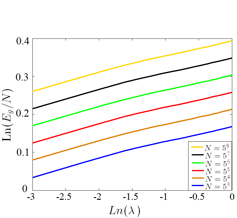
Figure 6: (Color online) The power law behavior of gap in terms of anisotropy parameter $\lambda\neq 0$ for $D=0$. Different colors correspond to various RG steps as indicated in the legend.

As can be seen in Fig. 5 although for all values of $D$ the gap is a function of $\lambda$ that vanishes at $\lambda=0$, but the way it vanishes depends on $D$ and is not universal. To extract these information, in Fig. 6 we produce a log-log plot of the gap versus $\lambda$ for $D=0$. Note that very small values of $\lambda\sim 10^{-3}$ are needed to extract the dependence of gap on $\lambda$. The linear dependence of the log-log plot suggests a perfect power-law dependence of the gap, $E_{g}\propto\lambda^{m}$, where the non-universal exponent $m$ actually does depend on $D$. This is analogous to the behavior of the corresponding 1D system den Nijs (1981) where in the absence of DM term one has $E_{g}\approx\lambda$. The BSRG for three-site problem in 1D with $D=0$ gives $E_{g}\propto\lambda^{0.63}$. In 2D square lattice Fig. 6 suggests that this exponent for $D=0$ is given as $E_{g}\approx\lambda^{0.4869}$. Note that the value of the exponent ($0.4869$) has finite size errors.

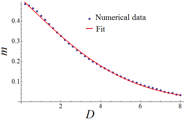
Figure 7: (Color online) Exponent $m$ of $E_{g}\sim\lambda^{m}$ which determines how does the gap vanish as a function of $\lambda$. This exponent variers with $D$. These values are extracted from 8th level RG step which converges within the precision of $10^{-5}$

By turning on the DM interaction $D$ as can be seen in Fig. 5 still the gap vanishes as $\lambda$ approaches zero. To quantify this, we repeat the above log-log analysis for various values of $D$, and extracting the corresponding exponent $m$ as a function of $D$, we obtain the set of data points in Fig. 7. As can be seen from Fig. 7 for larger $D$ the exponent becomes smaller. Using the following ansatz for the fit,

$$m=\exp(\alpha D^{2}+\beta D+\gamma),$$ (16)

gives, $\alpha=-0.02042\pm 0.00106$, $\beta=-0.1828\pm 0.00523$ and $\gamma=-0.6732\pm 0.00499$.

III.3 Analysis of the concurrence

So far we have established that for any $D$, the $\lambda=0$ repulsive line is a gapless line. This is consistent with a picture of underlying phase coherent super-fluid, albeit not limited to $D=0$, but also valid for nonzero values of $D$. The value of $D$ only affects the exponent $m$ that determines how fast the gap vanishes. Its repulsive nature indicates some form of instability towards a gapped state. Both positive and negative $\lambda$ sides are gapped states. Is the gap closing at $\lambda=0$ line a topological phase transition? In the $\lambda=0$ (isotropic) XY model, the non-analytic value of GMC is suggested as and indicator of the spin fluid phase in the 2D system Usman et al. (2015).

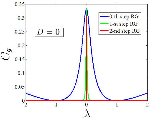
Figure 8: (Color online) GMC as a function of anisotropy parameter $\lambda$ in the absence of DM interaction in different RG steps. The non-vanishing GMC indicates that the gap closing at $\lambda=0$ is a topological phase transition.

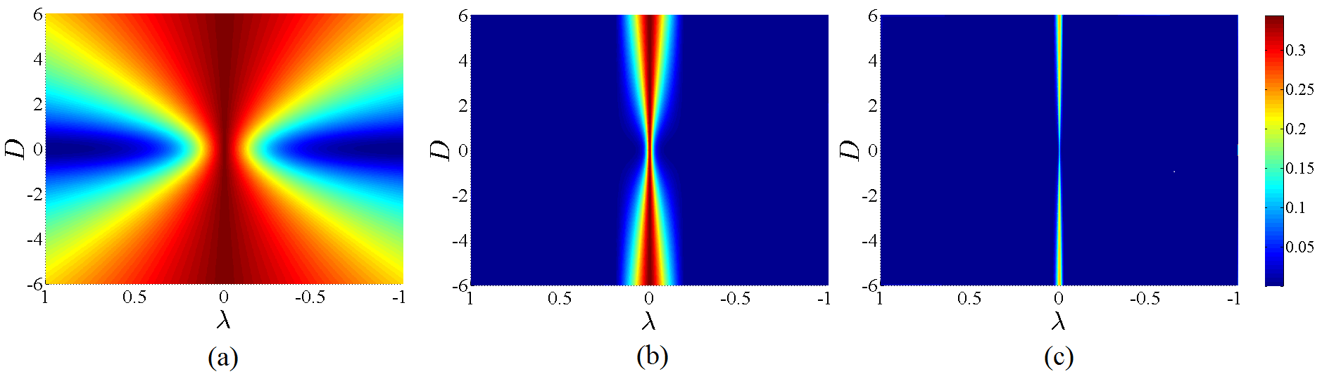
Figure 9: (Color online) Intensity map of GMC in the $(\lambda,D)$ plane for various RG steps: (a) 0-th RG step, (b) 1-st RG step and (c) 2-nd RG step. In the all values of DM interaction at the nontrivial point of $\lambda=0$ the GMC shows non-analytic behavior.

In Fig. 8 we have plotted the GMC versus anisotropy parameter $\lambda$ for the $D=0$ case. As can be seen by repeating the RG steps, the convergence can be attained very quickly, and the GMC at $\lambda=0$ becomes non-analytic. This suggest that the gap closing at $\lambda=0$ line is a topological phase transition Cho and Kim (2017). A nice feature of the above plot is the vanishing of GMS at $\lambda=\pm 1$ which corresponds to Ising-Kitaev limit polarized along $\hat{x}$ or $\hat{y}$ directions. For such a product state the entanglement must be zero.

To put the above picture in a global perspective, in Fig. 9 we plot intensity profile of GMC at first two steps of the RG process. This figure suggests that at the $\lambda=0$ line the gap-closing is accompanied by a change of topology Cho and Kim (2017).

IV Summary and discussion

The phase portrait of anisotropy 2DQXY model with DM interaction in Fig. 4 indicates that the DM interaction is irrelevant in the infrared limit. The $\lambda=0$ line is a gapless line that separates two gapped states for positive and negative $\lambda$. The analysis of concurrence in Fig. 9 suggest that the gap-closing transition at $\lambda=0$ is a topological phase transition Cho and Kim (2017). In the bosonic language, the gapless state at $\lambda=0$ corresponds to a super-fluid phase of underlying bosons Carrasquilla and Rigol (2012); Sachdev (2011), and vanishing of the gap can be attributed to the soft phase fluctuations of a super-fluid Sandvik and Hamer (1999). There are two ways to destroy the long range order in the phase variable: The well known way is by the BKT mechanism, i.e. the proliferation of vortices at elevated temperatures.

The second way to gap the super-fluid state is to stay at zero temperature but turn on the anisotropy $\lambda$. According to present study, as long as anisotropy $\lambda$ stays at zero, the DM interaction does not help with gapping the state. Having established that $\lambda\neq 0$ generates a gapped state for any $D$, the question is, what kind of gapped state is it? Is it topologically trivial or non-trivial? Fermionic representation of the problem in terms of Jordan-Wigner fermions coupled with the Chern-Simons gauge fields Fradkin (1989); Lopez et al. (1994); Fradkin (2013); Kumar et al. (2014) suggests that the gapped state is a topological superconductor Sedrakyan et al. (2017). The super-fluid picture at $\lambda=0$ (in the bosonic language) corresponds to a liquid of JW fermions coupled with CS gauge fields in the fermionic picture. In the fermionic language, the anisotropy parameter $\lambda$ triggers a superconducting pairing instability in the Fermi sear of JW fermions leading to a topologically non-trivial superconducting state of JW fermions Sedrakyan et al. (2017).

In our RG picture this can be understood as follows: Deep in the gapped phase, at the Ising-Kitaev fixed points, $\lambda=+(-)1$ the long distance behavior of the system is equivalent to a simple 2D Ising model polarized along $\hat{x}~{}(\hat{y})$ direction. The ground state at these fixed points is factorizable and this explains why in Fig. 8 the entanglement indicator at all RG steps gives zero. This means that at the Ising-Kitaev fixed point the Hamiltonian is given in terms of entirely commuting variables, and hence it has become purely classical (hence zero entanglement). The fact that entanglement at every RG step (i.e. for every system size) in Fig. 8 is zero, already indicates that it has been protected by some sort of topology, and therefore the resulting Ising degeneracy can be interpreted in a dual picture as topological degeneracy Fradkin (2017). At these fixed points the resulting classical 2D Ising model translates via celebrated Lieb-Schultz-Mattis mapping Mattis (2006) to a one-dimensional p-wave superconductor in modern terms. This is nothing but the well known Kitaev model of a topological superconductor. Therefore the ground states at the fixed points $\lambda=\pm 1$ is entitled to a winding number. Now moving slightly away from these fixed points and deforming the Hamiltonian in such a way that it ultimately returns to the fixed points upon enlarging the length scale, the topological number does not change, as there is no gap-closing as long as one does not hit the $\lambda=0$ repeller line. Therefore our real space RG is consistent with a non-trivial topological charge for the gapped states at $\lambda\neq 0$.

To summarize, we have considered the quantum XY model in 2D square lattice in the presence of DM interaction. The symmetry of problem allows us to obtain analytical expressions for the ground state doublet of this system which then enables us to set up a real space block spin RG. The DM interaction turns out to be irrelevant at long wave-lengths. The RG flow consists in a gapless repulsive $\lambda=0$ line, and two attractive $(\lambda=\pm 1,D=0)$ points corresponding to Ising-Kitaev limit. Non-analyticity of concurrence shows that the phase transition at $\lambda=0$ is of topological nature Cho and Kim (2017). The Ising Kitaev-limit enables us to assign a topological charge to the gapped phases at $\lambda\neq 0$. These features are very similar to corresponding 1D system Jafari (2017) and in agreement with results of studies based on JW fermions coupled with CS gauge fields Sedrakyan et al. (2017).

Appendix A Details of exact diagonalization of selected cluster in square lattice

In this appendix, details of the exact diagonalization for selected cluster in square lattice are presented. To reduce the dimension of ensuing matrix we employ group theory method. To obtain the eigenvalues (Eq. 2) and eigen-states (Eq. 4 and 5) first we consider the possible states of spin-1/2 system $2^{5}$ in cluster $P$. Each state of the cluster is in the following form,

$$|\alpha_{i}\rangle=|\sigma_{4},\sigma_{3},\sigma_{2},\sigma_{1},\sigma_{0}\rangle$$ (17)

where $i=1~{}...~{}32$ and $\sigma$ present the two possible values $\uparrow\downarrow$ in Fig. 1 . The basis in this 32 dimensional Hilbert space are as (for brevity in representation of basis states we drop $|\rangle$),

$$|\alpha_{1}\rangle=\uparrow\uparrow\uparrow\uparrow\uparrow,|\alpha_{2}\rangle=\uparrow\uparrow\uparrow\uparrow\downarrow,|\alpha_{3}\rangle=\uparrow\uparrow\uparrow\downarrow\uparrow,|\alpha_{4}\rangle=\uparrow\uparrow\downarrow\uparrow\uparrow,$$

$$|\alpha_{5}\rangle=\uparrow\downarrow\uparrow\uparrow\uparrow,|\alpha_{6}\rangle=\downarrow\uparrow\uparrow\uparrow\uparrow,|\alpha_{7}\rangle=\downarrow\uparrow\uparrow\uparrow\downarrow,|\alpha_{8}\rangle=\downarrow\uparrow\uparrow\downarrow\downarrow,$$

$$|\alpha_{9}\rangle=\downarrow\uparrow\downarrow\uparrow\downarrow,|\alpha_{10}\rangle=\downarrow\downarrow\uparrow\uparrow\downarrow,|\alpha_{11}\rangle=\uparrow\uparrow\uparrow\downarrow\downarrow,|\alpha_{12}\rangle=\uparrow\uparrow\downarrow\downarrow\uparrow,$$

$$|\alpha_{13}\rangle=\uparrow\downarrow\downarrow\uparrow\uparrow,|\alpha_{14}\rangle=\uparrow\downarrow\uparrow\uparrow\downarrow,|\alpha_{15}\rangle=\uparrow\downarrow\uparrow\downarrow\uparrow,|\alpha_{16}\rangle=\uparrow\uparrow\downarrow\uparrow\downarrow,$$

$$|\alpha_{17}\rangle=\downarrow\downarrow\downarrow\downarrow\uparrow,|\alpha_{18}\rangle=\downarrow\downarrow\downarrow\uparrow\downarrow,|\alpha_{19}\rangle=\downarrow\downarrow\uparrow\downarrow\downarrow,|\alpha_{20}\rangle=\downarrow\uparrow\downarrow\downarrow\downarrow,$$

$$|\alpha_{21}\rangle=\uparrow\downarrow\downarrow\downarrow\downarrow,|\alpha_{22}\rangle=\uparrow\downarrow\downarrow\downarrow\uparrow,|\alpha_{23}\rangle=\uparrow\downarrow\downarrow\uparrow\downarrow,|\alpha_{24}\rangle=\uparrow\downarrow\uparrow\downarrow\downarrow,$$

$$|\alpha_{25}\rangle=\uparrow\uparrow\downarrow\downarrow\downarrow,|\alpha_{26}\rangle=\downarrow\downarrow\downarrow\uparrow\uparrow,|\alpha_{27}\rangle=\downarrow\downarrow\uparrow\uparrow\downarrow,|\alpha_{28}\rangle=\downarrow\uparrow\uparrow\downarrow\downarrow,$$

$$|\alpha_{29}\rangle=\downarrow\uparrow\downarrow\downarrow\uparrow,|\alpha_{30}\rangle=\downarrow\uparrow\downarrow\uparrow\downarrow,|\alpha_{31}\rangle=\downarrow\downarrow\uparrow\downarrow\uparrow,|\alpha_{32}\rangle=\downarrow\downarrow\downarrow\downarrow\downarrow,$$

Now we proceed calculations by employing symmetry consideration to reduce 32 dimensional Hilbert space to smaller blocks in matrix representation. The + shape of cluster in Fig. 1. is invariant under rotations by $\frac{\pi}{2}$ which is denoted by $\mathcal{C}$ and then the rotation group is given by $\{\mathcal{C}^{0},\mathcal{C}^{1},\mathcal{C}^{2},\mathcal{C}^{3}\}$. The $\mathcal{C}$ operates on the site labels as,

$$\mathcal{C}=\left\{\begin{matrix}1\to 2\\ 2\to 3\\ 3\to 4\\ 4\to 1\\ \end{matrix}\right.\$$ (19)

By successive operation of $\mathcal{C}$ on a one state for e.i. $|\alpha_{3}\rangle$, the following pattern is obtained,

$$|3\rangle\xrightarrow{\mathcal{C}}|4\rangle\xrightarrow{\mathcal{C}}|5\rangle\xrightarrow{\mathcal{C}}|6\rangle\xrightarrow{\mathcal{C}}|3\rangle$$ (20)

which is the concise representation of

$$\mathcal{C}^{0}|3\rangle=|3\rangle,$$

$$\mathcal{C}^{1}|3\rangle=|4\rangle,$$

$$\mathcal{C}^{2}|3\rangle=|5\rangle,$$

$$\mathcal{C}^{3}|3\rangle=|6\rangle,$$

(21)

According to projection theorem in group theory we construct the symmetry adopted state in representation which is labeled by $n$ from an arbitrary state $|\phi\rangle$

$$|\psi^{(n)}\rangle\sim\left(\sum_{g}g\Gamma_{n}[g]\right)|\phi\rangle$$ (22)

where $g$ interprets the member of group and $\Gamma_{n}[g]$ denotes the $n$-th irreducible representation for element $g$ in the group. Our case is a rotation group and the irreducible representations of the cyclic group are tagged by means of three (angular momentum) $n=0,~{}\pm 1$. These are presented by $\{\omega^{0},~{}\omega^{n},~{}\omega^{2n},~{}\omega^{3n}\}$ where $\omega=\exp(i\pi/2)$. The $\Gamma_{n}(\mathcal{C}^{p})=\omega^{pn}$ is the well-set representation of above cyclic group. A symmetry adopted state build from e.i. $|3\rangle$ is,

$$\left(\mathcal{C}^{0}\omega^{0}+\mathcal{C}^{1}\omega^{n}+\mathcal{C}^{2}\omega^{2n}+\mathcal{C}^{3}\omega^{3n}\right)|3\rangle$$ (23)

where by applying Eq. 21, the obtained state is as,

$$|3\rangle+\omega^{n}|4\rangle+\omega^{2n}|5\rangle+\omega^{3n}|6\rangle$$ (24)

with $n$ is the angular momentum. By applying the same symmetry to every other states we obtain,

$$|7\rangle\xrightarrow{\mathcal{C}}|11\rangle\xrightarrow{\mathcal{C}}|14\rangle\xrightarrow{\mathcal{C}}|16\rangle\xrightarrow{\mathcal{C}}|7\rangle$$

$$|8\rangle\xrightarrow{\mathcal{C}}|10\rangle\xrightarrow{\mathcal{C}}|12\rangle\xrightarrow{\mathcal{C}}|13\rangle\xrightarrow{\mathcal{C}}|8\rangle$$

$$|18\rangle\xrightarrow{\mathcal{C}}|19\rangle\xrightarrow{\mathcal{C}}|20\rangle\xrightarrow{\mathcal{C}}|21\rangle\xrightarrow{\mathcal{C}}|18\rangle$$

$$|22\rangle\xrightarrow{\mathcal{C}}|26\rangle\xrightarrow{\mathcal{C}}|29\rangle\xrightarrow{\mathcal{C}}|31\rangle\xrightarrow{\mathcal{C}}|22\rangle$$

$$|23\rangle\xrightarrow{\mathcal{C}}|25\rangle\xrightarrow{\mathcal{C}}|27\rangle\xrightarrow{\mathcal{C}}|28\rangle\xrightarrow{\mathcal{C}}|23\rangle$$

$$|9\rangle\xrightarrow{C}|15\rangle\xrightarrow{C}|9\rangle$$

$$|24\rangle\xrightarrow{C}|30\rangle\xrightarrow{C}|24\rangle$$

$$|1\rangle\xrightarrow{C}|1\rangle,~{}~{}~{}~{}~{}|2\rangle\xrightarrow{C}|2\rangle$$

$$|17\rangle\xrightarrow{C}|17\rangle,~{}~{}~{}~{}~{}|32\rangle\xrightarrow{C}|32\rangle$$

The normalized states are as,

$$|\phi_{1}\rangle=|\alpha_{1}\rangle,$$

$$|\phi_{2}\rangle=|\alpha_{2}\rangle,$$

$$|\phi_{3}\rangle=\frac{1}{2}\left(|\alpha_{3}\rangle+|\alpha_{4}\rangle+|\alpha_{5}\rangle+|\alpha_{6}\rangle\right),$$

$$|\phi_{4}\rangle=\frac{1}{2}\left(|\alpha_{7}\rangle+|\alpha_{11}\rangle+|\alpha_{14}\rangle+|\alpha_{16}\rangle\right),$$

$$|\phi_{5}\rangle=\frac{1}{2}\left(|\alpha_{8}\rangle+|\alpha_{10}\rangle+|\alpha_{12}\rangle+|\alpha_{13}\rangle\right),$$

$$|\phi_{6}\rangle=\frac{1}{\sqrt{2}}\left(|\alpha_{9}\rangle+|\alpha_{15}\rangle\right),$$

$$|\phi_{7}\rangle=\frac{1}{2}\left(|\alpha_{18}\rangle+|\alpha_{19}\rangle+|\alpha_{20}\rangle+|\alpha_{21}\rangle\right),$$

$$|\phi_{8}\rangle=\frac{1}{2}\left(|\alpha_{22}\rangle+|\alpha_{26}\rangle+|\alpha_{29}\rangle+|\alpha_{31}\rangle\right),$$

$$|\phi_{9}\rangle=\frac{1}{2}\left(|\alpha_{23}\rangle+|\alpha_{25}\rangle+|\alpha_{27}\rangle+|\alpha_{28}\rangle\right),$$

$$|\phi_{10}\rangle=\frac{1}{\sqrt{2}}\left(|\alpha_{24}\rangle+|\alpha_{30}\rangle\right),$$

$$|\phi_{11}\rangle=|\alpha_{17}\rangle,$$

$$|\phi_{12}\rangle=|\alpha_{32}\rangle.$$

The same approach will lead to normalized state at $n=+1$ sector. Due to the time reversal symmetry the $n=-1$ sector has identical spectrum. The $n=+1$ sector normalized states are,

$$|\chi_{1}\rangle=\frac{1}{2}\left(|\alpha_{3}\rangle+\omega|\alpha_{4}\rangle+\omega^{2}|\alpha_{5}\rangle+\omega^{3}|\alpha_{6}\rangle\right),$$

$$|\chi_{2}\rangle=\frac{1}{2}\left(|\alpha_{7}\rangle+\omega|\alpha_{11}\rangle+\omega^{2}|\alpha_{14}\rangle+\omega^{3}|\alpha_{16}\rangle\right),$$

$$|\chi_{3}\rangle=\frac{1}{2}\left(|\alpha_{8}\rangle+\omega|\alpha_{10}\rangle+\omega^{2}|\alpha_{12}\rangle+\omega^{3}|\alpha_{13}\rangle\right),$$

$$|\chi_{4}\rangle=\frac{1}{2}\left(|\alpha_{18}\rangle+\omega|\alpha_{19}\rangle+\omega^{2}|\alpha_{20}\rangle+\omega^{3}|\alpha_{21}\rangle\right),$$

$$|\chi_{5}\rangle=\frac{1}{2}\left(|\alpha_{22}\rangle+\omega|\alpha_{26}\rangle+\omega^{2}|\alpha_{29}\rangle+\omega^{3}|\alpha_{31}\rangle\right),$$

$$|\chi_{6}\rangle=\frac{1}{2}\left(|\alpha_{23}\rangle+\omega|\alpha_{25}\rangle+\omega^{2}|\alpha_{27}\rangle+\omega^{3}|\alpha_{28}\rangle\right),$$

It should be noted that the other symmetry such as parity symmetry in the selected cluster is in the heart of the rotation symmetry. The other operator that we introduced is

$$\zeta=\prod_{i}\sigma^{z}_{i}$$ (28)

which operates as a constant of motion. Consider one arbitrary state with arrangements of spins of up and down. The operation of XY Hamiltonian on a selected arrangements does not change the value of $q$. The reason is that in the presence of the two consecutive $\sigma^{x}$ or $\sigma^{y}$ operator the total number of spin flip is even. This operator acts on the 32 basis of cluster and breaks it in two family with $\zeta=+1$ which consist of

$$|\alpha_{1}\rangle,|\alpha_{7}\rangle,|\alpha_{8}\rangle,|\alpha_{9}\rangle$$

$$|\alpha_{10}\rangle,|\alpha_{11}\rangle,|\alpha_{12}\rangle,|\alpha_{13}\rangle$$

$$|\alpha_{14}\rangle,|\alpha_{15}\rangle,|\alpha_{16}\rangle,|\alpha_{17}\rangle$$

$$|\alpha_{18}\rangle,|\alpha_{19}\rangle,|\alpha_{20}\rangle,|\alpha_{21}\rangle$$ (29)

and $\zeta=-1$

$$|\alpha_{2}\rangle,|\alpha_{3}\rangle,|\alpha_{4}\rangle,|\alpha_{5}\rangle$$

$$|\alpha_{6}\rangle,|\alpha_{22}\rangle,|\alpha_{23}\rangle,|\alpha_{24}\rangle$$

$$|\alpha_{25}\rangle,|\alpha_{26}\rangle,|\alpha_{27}\rangle,|\alpha_{28}\rangle$$

$$|\alpha_{29}\rangle,|\alpha_{30}\rangle,|\alpha_{31}\rangle,|\alpha_{32}\rangle.$$ (30)

By considering all the symmetries and constant of motion, it is possible to diagonalize Hamiltonian analytically for obtain the ground state and energy bands. For e.i. in $n=0$ sector the Hamiltonian of the system by considering above symmetries in $\zeta=1$ reduced to

$$H=\left[\begin{matrix}0&0&0&4J\lambda&0&0\\ 0&0&4J(1+iD)&0&0&0\\ 0&4J(1-iD)&0&0&4J\lambda&2\sqrt{2}J\lambda\\ 4J\lambda 0&0&0&0&4J(1+iD)&2\sqrt{2}J(1+iD)\\ 0&0&4J\lambda&4J(1-iD)&0&0\\ 0&0&2\sqrt{2}J\lambda&2\sqrt{2}J(1-iD)&0&0\\ \end{matrix}\right]$$

where the eigenvalues of above matrix of Hamiltonian are

$$e_{0}=-2J\sqrt{5(1+D^{2})+5\lambda^{2}+\eta},$$

$$e_{1}=-2J\sqrt{5(1+D^{2})+5\lambda^{2}-\eta},$$

$$e_{2}=e_{3}=0,$$

$$e_{4}=2J\sqrt{5(1+D^{2})+5\lambda^{2}-\eta},$$

$$e_{5}=2J\sqrt{5(1+D^{2})+5\lambda^{2}+\eta},$$

in which

$$\eta=\sqrt{\lambda^{4}+34\lambda^{2}(1+D^{2})+(1+D^{2})^{2}}$$ (32)

and the $e_{0}$ is the ground state.

References

- Berezinskii (1971) V. L. Berezinskii, Sov. Phys. JETP 32, 493 (1971).
- Kosterlitz and Thouless (1973) J. M. Kosterlitz and D. J. Thouless, Journal of Physics C: Solid State Physics 6, 1181 (1973).
- Fradkin (2013) E. Fradkin, Field Theories of Condensed Matter Physics (Cambridge University Press, 2013).
- Matsubara and Matsuda (1956) T. Matsubara and H. Matsuda, Rep. Prog. Theor. Phys. 16, 569 (1956).
- Berezinskii (1972) V. L. Berezinskii, Sov. Phys. JETP 34, 610 (1972).
- Oitma and Betts (1978) J. Oitma and D. D. Betts, Can. J. Phys. 56, 897 (1978).
- Tang (1988) S. Tang, Phys. Lett. A 129, 83 (1988).
- Drzewinski and Sznajd (1989) A. Drzewinski and J. Sznajd, Phys. Lett. A 138, 143 (1989).
- Ding and Makivić (1990) H.-Q. Ding and M. S. Makivić, Phys. Rev. B 42, 6827 (1990).
- Ding (1992) H. Q. Ding, Phys. Rev. B 45, 230 (1992).
- Ying et al. (1998) H. P. Ying, H. J. Luo, L. Schülke, and B. Zhang, Mod. Phys. Lett. B 12, 1237 (1998).
- Harada and Kawashima (1998) K. Harada and N. Kawashima, J. Phys. Soc. Jpn. 67, 2768 (1998).
- Carrasquilla and Rigol (2012) J. Carrasquilla and M. Rigol, Phys. Rev. A 86, 043629 (2012).
- Sachdev (2011) S. Sachdev, Quantum phase transitions (Cambridge University Press, 2011).
- Sandvik and Hamer (1999) A. W. Sandvik and C. J. Hamer, Phys. Rev. B 60, 6588 (1999).
- Kennedy et al. (1988) T. Kennedy, E. H. Lieb, and B. S. Shastry, Phys. Rev. Lett. 61, 2582 (1988).
- Dekeyser et al. (1977) R. Dekeyser, M. Reynaert, and M. H. Lee, Physica 68B, 627 (1977).
- Heidarian and Damle (2005) D. Heidarian and K. Damle, Phys. Rev. Lett. 95, 127206 (2005).
- Melko et al. (2005) R. G. Melko, A. Paramekanti, A. A. Burkov, A. Vishwanath, D. N. Sheng, and L. Balents, Phys. Rev. Lett. 95, 127207 (2005).
- Kim and W (2004) E. Kim and C. M. H. W, Science 305, 1941 (2004).
- Melko et al. (2004) R. G. Melko, A. W. Sandvik, and D. J. Scalapino, Phys. Rev. B 69, 100408 (2004).
- Gawiec and Grempel (1996) P. Gawiec and D. R. Grempel, Phys. Rev. B 54, 3343 (1996).
- Fradkin (1989) E. Fradkin, Phys. Rev. Lett. 63, 322 (1989).
- Lopez et al. (1994) A. Lopez, A. G. Rojo, and E. Fradkin, Phys. Rev. B 49, 15139 (1994).
- Wang (1991) Y. R. Wang, Phys. Rev. B 43, 3786 (1991).
- Kumar et al. (2014) K. Kumar, K. Sun, and E. Fradkin, Phys. Rev. B 90, 174409 (2014).
- Jafari (2017) S. A. Jafari, Phys. Rev. E 96, 012159 (2017).
- Sedrakyan et al. (2017) T. A. Sedrakyan, V. M. Galitski, and A. Kamenev, Phys. Rev. B 95, 094511 (2017).
- González et al. (2008) J. González, M. A. Martin-Delgado, G. Sierra, and A. H. Vozmediano, Quantum electron liquids and high-Tc superconductivity, Vol. 38 (Springer Science & Business Media, 2008).
- MARTÍN-DELGADO and SIERRA (1996) M. A. MARTÍN-DELGADO and G. SIERRA, International Journal of Modern Physics A 11, 3145 (1996), http://www.worldscientific.com/doi/pdf/10.1142/S0217751X96001516 .
- Dresselhaus et al. (2007) M. S. Dresselhaus, G. Dresselhaus, and A. Jorio, Group theory: application to the physics of condensed matter (Springer Science & Business Media, 2007).
- Amico et al. (2008) L. Amico, R. Fazio, A. Osterloh, and V. Vedral, Rev. Mod. Phys. 80, 517 (2008).
- Kargarian et al. (2007) M. Kargarian, R. Jafari, and A. Langari, Phys. Rev. A 76, 060304 (2007).
- Kargarian et al. (2008) M. Kargarian, R. Jafari, and A. Langari, Phys. Rev. A 77, 032346 (2008).
- Langari (2004) A. Langari, Phys. Rev. B 69, 100402 (2004).
- Song et al. (2013) X.-k. Song, T. Wu, and L. Ye, Quantum information processing 12, 3305 (2013).
- Song et al. (2014) X.-k. Song, T. Wu, S. Xu, J. He, and L. Ye, Annals of Physics 349, 220 (2014).
- Ma et al. (2011) F.-W. Ma, S.-X. Liu, and X.-M. Kong, Phys. Rev. A 84, 042302 (2011).
- Liu et al. (2016) X. Liu, W. Cheng, and J.-M. Liu, Scientific reports 6 (2016).
- Kitaev and Preskill (2006) A. Kitaev and J. Preskill, Physical review letters 96, 110404 (2006).
- Jiang et al. (2012) H.-C. Jiang, Z. Wang, and L. Balents, Nat Phys 8, 902–905 (2012).
- Cho and Kim (2017) J. Cho and K. W. Kim, Scientific reports 7, 2745 (2017).
- Bennett et al. (1996) C. H. Bennett, D. P. DiVincenzo, J. A. Smolin, and W. K. Wootters, Physical Review A 54, 3824 (1996).
- Hill and Wootters (1997) S. Hill and W. K. Wootters, Phys. Rev. Lett. 78, 5022 (1997).
- Strogatz (2014) S. H. Strogatz, Nonlinear dynamics and chaos: with applications to physics, biology, chemistry, and engineering (Westview press, 2014).
- den Nijs (1981) M. P. M. den Nijs, Phys. Rev. B 23, 6111 (1981).
- Usman et al. (2015) M. Usman, A. Ilyas, and K. Khan, Phys. Rev. A 92, 032327 (2015).
- Fradkin (2017) E. Fradkin, Journal of Statistical Physics 167, 427 (2017).
- Mattis (2006) D. C. Mattis, The theory of magnetism made simple (World Scientific, 2006).