Subgap states in two dimensional spectroscopy of unconventional superconductors using graphene

Abstract

The two-dimensional nature of graphene makes it an ideal platform to explore proximity-induced unconventional planar superconductivity and the possibility of topological superconductivity. Using Green’s functions techniques, we study the transport properties of a finite size ballistic graphene layer placed between a normal state electrode and a graphene lead with proximity-induced unconventional superconductivity. Our microscopic description of such a junction allows us to consider the effect of edge states in the graphene layer and the imperfect coupling to the electrodes. The tunnel conductance through the junction and the spectral density of states feature a rich interplay between graphene’s edge states, interface bound states formed at the graphene–superconductor junction, Fabry-Pérot resonances originated from the finite size of the graphene layer, and the characteristic Andreev surface states of unconventional superconductors. Within our analytical formalism, we identify the separate contribution from each of these subgap states to the conductance and density of states. Our results show that graphene provides an advisable tool to determine experimentally the pairing symmetry of proximity-induced unconventional superconductivity.

I Introduction

Unconventional superconductivity involves all pairing states that deviate from the ordinary $s$-wave, spin-singlet Cooper pairsSigrist and Ueda (1991), and are thus classified according to the symmetry of their order parameter. For example, high-$T_{c}$ superconductors feature an anisotropic $d$-wave spin-singlet pairing stateKashiwaya and Tanaka (2000); Lee et al. (2006) and there is increasing evidence for the compounds UPt₃ and Sr₂RuO₄ to be spin-triplet chiral $p$-wave superconductorsMackenzie and Maeno (2003); *Maeno_2012; *Kallin_2012. Recently, topological superconductorsRead and Green (2000) have triggered an intense research activity as they host gapless Majorana surface states, a candidate for fault-tolerant quantum computingIvanov (2001); Alicea (2012); *Beenakker_Majorana; *DasSarma_Majorana. Topological superconductivity can be artificially engineered in proximity-induced semiconductor nanowiresLutchyn et al. (2010); Oreg et al. (2010); Potter and Lee (2010); *Potter_2011 or naturally arises on chiral superconductorsKallin and Berlinsky (2016). A chiral superconducting state has also been proposed for other systems, including graphene, where the unconventional superconductivity can come from repulsive interactionsNandkishore et al. (2012); Black-Schaffer (2012); Black-Schaffer and Honerkamp (2014) or be induced by proximity to an electron-doped oxide superconductorDi Bernardo et al. (2017). Tunneling conductance measurements at normal metal–superconductor junctions are a very useful tool to detect signatures of all these types of unconventional superconductivityKashiwaya and Tanaka (2000). In a ballistic junction, transport at voltages below the superconducting gap is mediated by Andreev reflections, where incident electrons are converted into holes in the normal metal creating Cooper pairs in the superconductorBlonder et al. (1982); Klapwijk and Ryabchun (2014). The presence of surface states in unconventional superconductors is connected to resonance peaks in the Andreev reflection probability, resulting in conductance peaks below the superconducting gapTanaka and Kashiwaya (1995); Kashiwaya et al. (1995, 1996); Honerkamp and Sigristt (1998); Lu et al. (2016); Burset et al. (2017).

Unfortunately, tunneling spectroscopy of subgap resonances presents several experimental challenges, specially for nanoscale devicesKlapwijk and Ryabchun (2014). When considering hybrid junctions where the reservoirs and the intermediate scattering region are built from different materials, as sketched in Fig. 1(a), each interface between the intermediate region and the reservoirs may present a different transmissionWiedenmann et al. (2017). Additionally, quantum-coherent transport across the junction results in the emergence of Fabry-Pérot resonancesLiang et al. (2001); Kretinin et al. (2010). All these effects can mask the experimental detection of novel phenomena associated to unconventional superconductivityKlapwijk and Ryabchun (2014). However, recent experimental advances involving graphene-based nanoscale devices provide new ways to circumvent these challenges.

Graphene is a two-dimensional Dirac semimetal with high carrier mobilityDas Sarma et al. (2011); Rozhkov et al. (2011); Wehling et al. (2014). High-quality graphene nanoscale transistors have been achievedXia et al. (2011); *Avouris_2012 and fabrication of graphene nanoribbons with well-defined edges is an experimental possibilityDrost et al. (2014); *Liljeroth_2015. Early reports of graphene-based Josephson junctions were assumed to work in the diffusive regime with low-transmitting interfacesHeersche et al. (2007); *Miao_2007; *Shailos_2007; *Andrei_2008. Recent experiments, however, have achieved good quality ballistic graphene–superconductor contactsRickhaus et al. (2012); Calado et al. (2015); Ben Shalom et al. (2016). In particular, encapsulation in hexagonal boron nitride provides high-quality transparent junctions that work in the ballistic regimeCalado et al. (2015); Ben Shalom et al. (2016). Control over the independent doping of the graphene layer has allowed to measure specular Andreev reflectionsEfetov et al. (2016)–an unusual type of Andreev process that only manifests when the doping is smaller than the applied voltage and the superconducting gapBeenakker (2006). Advances in experimental control of graphene devices are leading to a series of remarkable works reporting spectroscopy of Andreev bound states in Josephson junctionsDirks et al. (2011), splitting of Cooper pairsTan et al. (2015), and possible proximity-induced superconductivity in graphene, either by growing graphene layers on superconductorsTonnoir et al. (2013) or by doping it with adatomsLudbrook et al. (2015); Chapman et al. (2016). Indeed, the peculiar hexagonal lattice of graphene allows for the formation of unconventional pairing correlationsUchoa and Castro Neto (2007); Jiang et al. (2008); Nandkishore et al. (2012); Black-Schaffer (2012). Graphene has been recently grown on top of unconventional (non-chiral) $d$-wave superconductors, revealing an interesting induced $p$-wave pairing stateDi Bernardo et al. (2017). Additionally, a recent experiment reports evidence of intrinsic unconventional superconductivity in graphene superlatticesCao et al. (2018). More experimental and theoretical work is required to fully understand the emergent unconventional superconductivity in graphene and determine if it is chiral and topological.

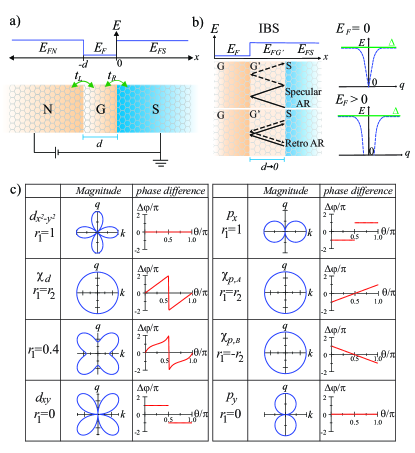
Figure 1: Graphene N-G-S junction. (a) Schematic of the N-G-S junction, including the energy profile. (b) IBS are formed at the G-S junction and can be interpreted as standing waves located at an intermediate graphene layer of width $d\!\rightarrow\!0$ (left panel). Sequences of Andreev specular and retro reflection processes involved in the formation of IBS are sketched: (solid) dashed arrows represent group velocities for (electron-) hole-like quasiparticles. The right panel shows the dispersion relation for the IBS when the superconductor is conventional $s$-wave. (c) Order parameter and angle dependence of the phase difference for the $d$-wave and $p$-wave symmetries considered. See text for more details.

In this work, we analyze the transport properties of ballistic junctions consisting of a finite graphene layer contacted by a normal state and a superconducting macroscopic lead [cf. Fig. 1(a)]. Within our model, we study the most representative two-dimensional unconventional superconductors, including nodal $d$-wave and chiral $p$- and $d$-wave pairing states, and the exotic superconducting states induced by graphene’s lattice. Our combination of scattering and microscopic Green’s function techniques allows us to go beyond previous works in graphene-based superconducting hybridsBeenakker (2006); Bhattacharjee and Sengupta (2006); Akhmerov and Beenakker (2007); Tkachov (2007); Linder and Sudbø (2007, 2008); Burset et al. (2008); Black-Schaffer and Doniach (2008); Burset et al. (2009); feng Sun and Xie (2009); Gómez et al. (2012) by including many of the most relevant experimental issues appearing at nanoscale graphene–superconductor junctions. Namely, by considering a finite size graphene layer we take into account the Fabry-Pérot resonances (FPR) present in experiments. Additionally, we describe imperfect coupling between the graphene layer and the reservoirs –including the effect of graphene’s zigzag edge states (ZZES)– and analyze the effect of doping the layer close or away from the Dirac point. As a result, we present differential conductance calculations with very rich subgap features, where the unconventional surface Andreev bound states (SABS) at the edge of the superconductor are mixed with FPRs, graphene’s zigzag edge states, and interface bound states (IBS) formed at the graphene–superconductor junctionBurset et al. (2009), see Fig. 1(b). We analytically describe the contribution of each process to the density of states (DOS) and differential conductance. We thus analyze the optimal conditions for the use of graphene to detect signatures of unconventional superconductivity.

The rest of the paper is organized as follows. In Sec. II we introduce our model and derive the main formulas for transport observables. We describe the spectral properties of G-S and N-G-S junctions in Sec. III and Sec. IV, respectively. Next, in Sec. V, we discuss the tunneling spectroscopy of unconventional superconductors. We present our conclusions in Sec. VI. The details of some of the model calculations are given in the Appendix A and B.

II Model

Our system consists of a graphene sheet (G) of length $d$ and width $W$ connected to reservoirs as sketched in Fig. 1(a). We consider transport along the $x$-direction and assume that $W\!\gg\!d$, so that there is translational invariance along the graphene–reservoir interfaces. The left and right semi-infinite graphene contacts are in the normal (N) and superconducting (S) states, respectively. Low-energy excitations of the coupled system are described by the Dirac-Bogoliubov-de Gennes (DBdG) equations

$$\begin{pmatrix}(\hat{H}_{\pm}-\varepsilon_{F}\hat{\sigma}_{0})\hat{s}_{0}&\hat{\Delta}\hat{\sigma}_{0}\\ \hat{\Delta}^{\dagger}\hat{\sigma}_{0}&(\varepsilon_{F}\hat{\sigma}_{0}-\hat{H}_{\pm})\hat{s}_{0}\end{pmatrix}\begin{pmatrix}\phi_{e}\\ \phi_{h}\end{pmatrix}\!=\!E\begin{pmatrix}\phi_{e}\\ \phi_{h}\end{pmatrix},$$ (1)

with $E\!\geq\!0$ the excitation energy and where the Pauli matrices $\hat{\sigma}_{\nu}$ ($\hat{s}_{\nu}$), with $\nu\!=\!0,1,2,3$, act in lattice (spin) space. The electrostatic potential of each region can be independently fixed and we take $\varepsilon_{F}\!=\!E_{FN},E_{F},E_{FS}$ for regions N, G, and S, respectively. In Eq. (1), we have decoupled graphene’s valley degree of freedom by assuming that the pair potential couples electrons and holes from different valleysBeenakker (2006, 2008). For each valley, we use the Dirac Hamiltonian $\hat{H}_{\pm}\!=\!-iv_{F}\partial_{x}\hat{\sigma}_{1}\pm v_{F}q\hat{\sigma}_{2}$, with $v_{F}$ the Fermi velocity and $q$ the conserved component of the wave vector parallel to the interfaces. Owing to such valley decoupling, we initially describe $\hat{H}_{+}$ only and later we discuss the role of the other valley.

The superconducting order parameter is only non-zero in region S, i.e., $\hat{\Delta}(\theta,x)\!=\!\hat{\Delta}(\theta)\Theta(x)$, with $\Theta(x)$ the Heaviside function, $\theta\!=\!\sin^{-1}(q/k_{FS})$ the angle in reciprocal space and $k_{F}$ the Fermi wave vector. We only consider spin-degenerate unconventional superconductors which allows us to decouple the spin degree of freedom in Eq. (1)Sigrist and Ueda (1991); Honerkamp and Sigristt (1998); Burset et al. (2014). Indeed, for spin-singlet states, we have $\hat{\Delta}(\theta)\!=\!\Delta(\theta)\mathrm{e}^{i\phi}(i\hat{s}_{2})$, with $\phi$ the global $U(1)$ gauge phase. Analogously, for spin-triplet superconductors we take $\hat{\Delta}(\theta)\!=\!\mathrm{e}^{i\phi}\mathbf{d}(\theta)\cdot\hat{\mathbf{s}}(i\hat{s}_{2})$, with the odd vector function $\mathbf{d}(\theta)\!=\!-\mathbf{d}(\pi\!-\!\theta)$. As long as the vector $\mathbf{d}$ is perpendicular ($\mathbf{d}\!\propto\!\hat{\mathbf{z}}$) or parallel to the $x-y$ graphene plane, the spin degree of freedom can be decoupled in Eq. (1). In this equation, the pairing is proportional to the identity matrix in lattice space, $\hat{\sigma}_{0}$, since we consider only on-site induced superconductivity in the graphene latticeBurset et al. (2008).

Under these approximations, the resulting DBdG equations written in Nambu (particle-hole) and lattice spaces read as $\check{H}\psi\!=\!E\psi$. Specifically,

$$\begin{pmatrix}v_{F}\mathbf{k}_{\alpha}\cdot\hat{\mathbf{\sigma}}-\mu\hat{\sigma}_{0}&\Delta(\theta_{\alpha})\mathrm{e}^{i\phi}\hat{\sigma}_{0}\\ \Delta^{\ast}(\theta_{\alpha})\mathrm{e}^{-i\phi}\hat{\sigma}_{0}&\mu\hat{\sigma}_{0}-v_{F}\mathbf{k}_{\alpha}\cdot\hat{\mathbf{\sigma}}\end{pmatrix}\begin{pmatrix}\phi_{\alpha}^{e}\\ \phi_{\alpha}^{h}\end{pmatrix}\!=\!E\begin{pmatrix}\phi_{\alpha}^{e}\\ \phi_{\alpha}^{h}\end{pmatrix},$$ (2)

with $\alpha\!=\!\pm$ for right and left movers, respectively. We notice here that, since the lattice is acting as a pseudo-spin degree of freedom, the reduced Hamiltonian of Eq. (2) is also suitable to describe induced pairing amplitudes with an structure in lattice spaceUchoa and Castro Neto (2007); Black-Schaffer and Doniach (2007); Jiang et al. (2008); Di Bernardo et al. (2017), with the appropriate redefinition of the pair potential.

To take into account the sign change of the triplet state with the wave vector, we only consider $k_{x}\!\geq\!0$ and define $\mathbf{k}_{\alpha}\!=\!(\alpha k_{x},q)$. We thus set $\theta_{+}\!=\!\theta$ and $\theta_{-}\!=\!\pi\!-\!\theta$ for right and left movers, respectively. The pair potential adopts the general form

$$\Delta(\theta_{\pm})=\Delta_{0}\left[r_{1}\cos(n\theta_{\pm})+ir_{2}\sin(n\theta_{\pm})\right],$$ (3)

with $\Delta_{0}\!\geq\!0$ the potential amplitude and $r_{2}^{2}\!=\!1\!-\!r_{1}^{2}$ the relative value of real and imaginary parts of the pair potential. The integer $n\!=\!0,1,2,\dots$ determines the orbital symmetry of the pairing state, i.e., the values $n\!=\!0,2$ correspond $s$- and $d$-wave states, respectively, while $n\!=\!1$ represents a $p$-wave state. More details about Eq. (2) and its solutions can be found in the Appendix A.

The retarded/advanced Green functions associated to the Hamiltonian in Eq. (2) satisfies the non-homogeneous DBdG equation

$$\left[\check{H}-(E\pm i0^{+})\check{I}\right]\check{g}_{q}^{r,a}(x,x^{\prime})=\delta\left(x-x^{\prime}\right)\check{I}\text{,}$$ (4)

where $\check{g}_{q}^{r,a}(x,x^{\prime})$ is the Fourier transform of the spatial Green function on the coordinates parallel to the interfaces, $\check{I}$ is the four-dimensional identity matrix and $\check{H}$ is the DBdG Hamiltonian given by Eq. (2). The unperturbed Green’s function $\check{g}_{q}^{r,a}(x,x^{\prime})$ is obtained combining asymptotic solutions that obey boundary conditions at the edges of a finite length graphene sheet, following a generalization of the method developed in Refs. McMillan, 1968; Furusaki and Tsukada, 1991; Kashiwaya and Tanaka, 2000; Herrera et al., 2010; Burset et al., 2015; Crépin et al., 2015; Breunig et al., 2018 for unconventional superconductors and described in Appendix B.

The Green functions of the coupled system $\check{G}$ are calculated by means of an algebraic Dyson equation of the formHerrera et al. (2010); Gomez (2011)

$$\check{G}_{q,ij}^{r,a}=\check{g}_{q,ij}^{r,a}+\check{g}_{q,ik}^{r,a}\check{\Sigma}_{kl}\check{G}_{q,lj}^{r,a}\text{,}$$ (5)

with short-hand notation $\check{g}_{q,ij}^{r,a}\!=\!\check{g}_{q}^{r,a}(x_{i},x_{j}^{\prime})$. The self-energies $\check{\Sigma}_{kl}$ ($k\neq l$) represent the hopping matrix between two different regionsHerrera et al. (2010). For the zigzag boundary conditions adopted in this work, opposite edges of the graphene layer correspond to atoms from a different sublattice. This leads to a specific form of the hopping matrix as defined below.

II.1 Transport observables

The spectral density of states is calculated from the retarded Green function as

$$\mathcal{A}_{q}(x,E)=-\frac{1}{\pi}\operatorname{Im}\left\{\mathrm{Tr}\check{G}_{q,ee}^{r}(x,x,E)\right\},$$ (6)

where the trace is taken over the electron-electron component in Nambu space. The local density of states (DOS) is given by

$$\rho(x,E)=\sum_{q,\sigma}\mathcal{A}_{q}(x,E).$$ (7)

The current for the setup sketched in Fig. 1(a) is obtained following the Hamiltonian approachCuevas et al. (1996); Gomez (2011). We compute the charge tunneling between the regions from the tight-binding Hamiltonian

$$\hat{H}=\hat{H}_{L}+\hat{H}_{C}+\hat{H}_{R}+\hat{H}_{T_{L}}+\hat{H}_{T_{R}}\text{,}$$ (8)

where $\hat{H}_{i=L,C,R}$ are the unperturbed Hamiltonians, and $\hat{H}_{T_{L,R}}$ is the tunneling Hamiltonian of the form

$$\hat{H}_{T_{L}} =\sum_{q,\sigma}t_{L}c_{q,LA\sigma}^{\dagger}\psi_{q,B\sigma}(-d)+\text{h.c.},$$ (9)

$$\hat{H}_{T_{R}} =\sum_{q,\sigma}t_{R}c_{q,RB\sigma}^{\dagger}\psi_{q,A\sigma}(0)+\text{h.c.},$$ (10)

where $c_{q,\nu j\sigma}$ and $\psi_{q,j}(x)$, with $\nu=L,R$ and $j=A,B$, are annihilation for electrons at the edges of the $L$,$R$,$C$ regions with parallel momentum $q$. The average current through the left interface is given by

$$I=-e\left\langle\frac{d}{d\tau}\hat{N}_{L}\right\rangle$$ (11)

$$=\frac{ie}{h}t_{L}\sum\limits_{q,\sigma}\left(\left\langle\hat{c}_{q,LA\sigma}^{{\dagger}}\hat{\psi}_{q,B\sigma}(-d)\right\rangle-\left\langle\hat{\psi}_{q,B\sigma}^{\dagger}(-d)\hat{c}_{q,LA\sigma}\right\rangle\right).$$

This average can be expressed in terms of the Keldysh or non-equilibrium Green functions defined as

$$\check{G}_{q,ij}^{\alpha\beta}\left(\tau_{\alpha},\tau_{\beta}^{\prime}\right)=-i\left\langle\hat{T}\left[\hat{D}_{q,i}\left(\tau_{\alpha}\right)\hat{D}_{q,j}^{{\dagger}}\left(\tau_{\beta}^{\prime}\right)\right]\right\rangle\text{,}$$ (12)

$$\hat{D}_{q,i}^{{\dagger}}\left(\tau\right)=\left(\hat{d}_{q,iA\uparrow}^{{\dagger}}\left(\tau\right),\hat{d}_{q,iB\uparrow}^{{\dagger}}\left(\tau\right),\hat{d}_{q,iA\downarrow}\left(\tau\right),\hat{d}_{q,iB\downarrow}\left(\tau\right)\right),$$

where $i,j=L,C,C^{\prime},R$, $\ \hat{d}_{q,Lj\sigma}(\tau)=\hat{c}_{q,Lj\sigma}(\tau)$, $\hat{d}_{q,Cj\sigma}(\tau)=\hat{\psi}_{q,j\sigma}(-d,\tau)$, $\hat{d}_{q,C^{\prime}j\sigma}(\tau)=\hat{\psi}_{q,j\sigma}(0,\tau)$, $\hat{d}_{q,Rj\sigma}(\tau)=\hat{c}_{q,Rj\sigma}(\tau)$, superscripts $\alpha,\beta$ correspond to the temporal branches of the Keldysh contour and $\hat{T}$ is the Keldysh time-ordering operator. Then, the current evaluated at the left juncture reduces to

$$I=\frac{e}{h}\sum\limits_{q,\sigma}\int\mathrm{d}E\mathrm{Tr}\left(\check{\tau}_{z}\check{t}_{L}\left[\check{g}_{q,L}^{+-}\check{t}_{L}^{{\dagger}}\check{G}_{q,CC}^{-+}-\check{g}_{q,L}^{-+}\check{t}_{L}^{{\dagger}}\check{G}_{q,CC}^{+-}\right]\right)\text{,}$$

where $\check{t}_{L,R}=\check{\Sigma}_{LC,C^{\prime}R}=(t_{L,R}/2\hat{\tau}_{z})(\hat{\sigma}_{x}+i\hat{\sigma}_{y})$ are the coupling self-energies, $\check{g}_{q,L}^{\gamma=+-,-+}$ corresponds to the non-equilibrium Green functions for the left uncoupled electrode evaluated at $x=x^{\prime}=-d$, and $\check{G}_{q,CC}^{\gamma}$ is the non-equilibrium Green function of the coupled system evaluated at $x=x^{\prime}=-d+0^{+}$. The last expression can be written in terms of the retarded/advanced Green functions by means of the following Dyson equation that contains information of the full region at the right of the left juncture

$$\check{G}_{q,CC}^{\gamma} = \check{G}_{q,CC}^{r}\check{t}_{L}\check{g}_{q,L}^{\gamma}\check{t}_{L}^{{\dagger}}\check{G}_{q,CC}^{a}+$$

$$\check{G}_{q,CC^{\prime}}^{r}\check{t}_{R}^{{\dagger}}\check{g}_{q,R}^{\gamma}\check{t}_{R}\check{G}_{q,C^{\prime}C}^{a},$$

with $\check{g}_{q,i}^{+-}\!=\!2\pi i\check{\rho}_{q,i}\check{f}_{i}$, $\check{g}_{i}^{-+}\!=\!-2\pi i\check{\rho}_{q,i}\left(\hat{\tau}_{0}\hat{\sigma}_{0}-\check{f}_{i}\right)$ and $\check{\rho}_{q,i}\!=\!\mp\operatorname{Im}(\check{g}_{q,i}^{r(a)})/\pi$. The Fermi-Dirac distribution matrix for a voltage $V_{i}$ applied to electrode $i$ is defined as $\check{f}_{i}(\varepsilon,V)\!=\!\mathrm{diag}(f(\varepsilon\!-\!eV_{i})\hat{\sigma}_{0},f(\varepsilon\!+\!eV_{i})\hat{\sigma}_{0})$, with $f({\varepsilon})\!=\![1\!+\!\exp{(\beta\varepsilon)}]^{-1}$ and $\beta$ the inverse temperature. Finally, the current is given by

$$I=\sum_{q}I_{q}=\frac{4\pi^{2}e}{h}\sum\limits_{q,\sigma}\int\mathrm{d}E\mathrm{Tr}\left\{\tau_{z}\check{t}_{L}\check{\rho}_{q,L}\left({}\right.\right.$$

$$\left[\check{f}_{L}\check{t}_{L}^{{\dagger}}\check{G}_{q,CC}^{r}\check{t}_{L}\check{\rho}_{q,L}-\check{t}_{L}^{{\dagger}}\check{G}_{q,CC}^{r}\check{t}_{L}\check{\rho}_{q,L}\check{f}_{L}\right]\check{t}_{L}^{{\dagger}}\check{G}_{q,CC}^{a}+$$

$$\left.\left.\left[\check{f}_{L}\check{t}_{L}^{{\dagger}}\check{G}_{q,CC^{\prime}}^{r}\check{t}_{R}^{{\dagger}}\check{\rho}_{q,R}-\check{t}_{L}^{{\dagger}}\check{G}_{q,CC^{\prime}}^{r}\check{t}_{R}^{{\dagger}}\check{\rho}_{q,R}\check{f}_{R}\right]\check{t}_{R}\check{G}_{q,C^{\prime}C}^{a}\right)\right\}.$$

The differential conductance as a function of $q$ reads

$$\sigma_{q}=\frac{\partial I_{q}}{\partial V}=\sigma_{q,A}+\sigma_{q,Q},$$ (14)

where $\sigma_{q,A}$ is the contribution of Andreev processes,

$$\sigma_{q,A}=\frac{16e^{2}}{h}\mathrm{Tr}\left[\mathrm{Re}\left\{\bar{\rho}_{q,Lee}\hat{G}_{q,CCeh}^{r}\bar{\rho}_{q,Lhh}\hat{G}_{q,CChe}^{a}\right\}\right],$$ (15)

with $\bar{\rho}_{q,i\mu\nu}$ the Nambu component of the matrix $\bar{\rho}_{q,i}\!=\!\pi\check{t}_{i}\check{\rho}_{q,i}\check{t}_{i}^{\dagger}$. The contribution $\sigma_{q,Q}$ due to quasiparticles is given by

$$\sigma_{q,Q}=\frac{8e^{2}}{h}\mathrm{Tr}\left[\mathrm{Re}\left\{\bar{\rho}_{q,Lee}\left({}\right.\right.\right.$$ (16)

$$\left.\left.\hat{G}_{q,CC^{\prime}ee}^{r}\left[\bar{\rho}_{q,Ree}\hat{G}_{q,C^{\prime}Cee}^{a}-\bar{\rho}_{q,Reh}\hat{G}_{q,C^{\prime}Che}^{a}\right]\right.\right.$$

$$-\left.\left.\left.\hat{G}_{q,CC^{\prime}eh}^{r}\left[\bar{\rho}_{q,Rhe}\hat{G}_{q,C^{\prime}Cee}^{a}-\bar{\rho}_{q,Rhh}\hat{G}_{q,C^{\prime}Che}^{a}\right]\right)\right\}\right].$$

We use a highly doped semi-infinite graphene lead in order to model the normal electrode. Conductances are normalized to the normal-state graphene conductance. Eq. (14) provides a generalized formula to calculate the differential conductance in graphene-superconductor hybrid structures.

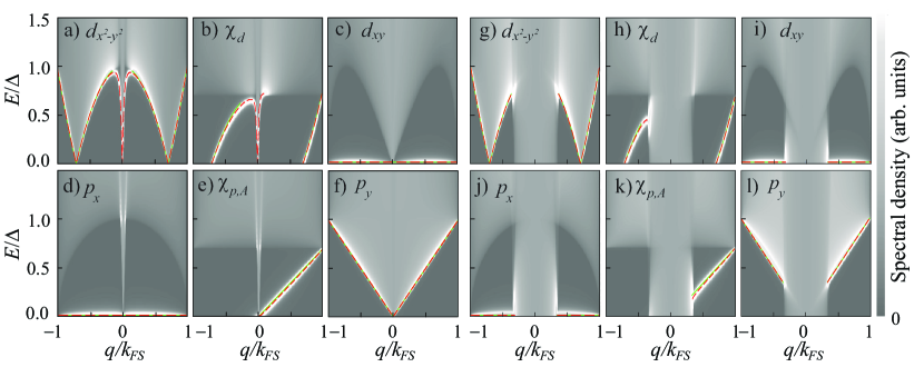
Figure 2: Spectral density of states of a semi-infinite graphene sheet coupled to a semi-infinite anisotropic superconductor evaluated at the interface. $E_{F}=0$ for figures (a-f) and $E_{F}=10\Delta$ for (g-l). SABS (solid green lines) and IBS (dashed red lines) are depicted for the different symmetries.

III Spectral properties of graphene-superconductor junctions

The spectral properties of the full N-G-S system contain information from many different sources: ZZES, FPR, IBS and SABS. We analyze the N-G-S setup numerically in the next section. In some particular cases, however, we can obtain simple analytical formulas for the contribution from some of these states. In this section, we consider a simpler setup where the left electrode is removed, resulting in a graphene-superconductor (G-S) junction, see Fig. 1(b). The coupled Green function is given by Dyson’s equation introduced in Eq. (5), see Appendix B for more details. The denominator of this perturbed Green function encodes information about the different states present in the junction. By finding its zeros, we obtain the dispersion relation of the induced resonances in the junction. In this section, we assume a perfect coupling between the graphene layer and the superconductor to avoid the formation of ZZES at the G-S interface. However, for finite graphene layers there is another ZZES at the opposite edge. Analyzing the Green function at the middle of the graphene layer, we can minimize the impact of ZZES on the spectrum and focus on the other resonances.

First, proximity-induced pairing from an unconventional superconductor always manifests with the emergence of SABS with a dispersion relation given byLöfwander et al. (2001)

$$E_{\text{SABS}}=\pm\left|\Delta\left(\theta\right)\right|\cos\Delta\varphi/2,$$ (17)

with $\Delta\varphi\!=\!\varphi_{+}-\varphi_{-}$ the phase difference between the pair potentials $\Delta(\theta_{+})$ and $\Delta(\theta_{-})$ defined in Eq. (3). Eq. (17) takes different forms depending on the symmetry of the pair potential, cf. Fig. 1(c). For symmetries $s,d_{x^{2}-y^{2}}$ and $p_{y}$ ($\Delta\varphi\!=\!0$) we get $E\!=\!\pm\left|\Delta\left(\theta\right)\right|$. For $d_{xy}$ and $p_{x}$ symmetries, we have $\Delta\varphi\!=\!\pi$ which corresponds to zero energy states (ZES) $E\!=\!0$. Chiral symmetries feature an angle dependence as follows: chiral $d$-wave symmetry $\chi_{d}$ ($\Delta\varphi\!=\!4\theta$) results in $E\!=\!\pm\left|\Delta\left(\theta\right)\right|\cos 2\theta$, and chiral $p$-wave $\chi_{p}$ ($\Delta\varphi\!=\!\mathrm{sgn}(r_{1})2\theta+\pi$) gives $E\!=\!\pm\left|\Delta\left(\theta\right)\right|\sin\theta$.

In addition to the SABS, the special properties of the graphene layer lead to the emergence of IBSBurset et al. (2009), which describe how the linear dispersion of graphene adapts to the presence of the gapped superconducting density of states. Moreover, a finite graphene layer will feature discrete energy bands, labeled here FPR, and ZZES. A general expression that describes IBS and FPR reads as

$$E_{\text{G-S}}=$$ (18)

$$\pm\left(\frac{C\cos\left(\Delta\varphi/2\right)+i\sin\left(\Delta\varphi/2\right)}{\sqrt{C^{2}-1}}\right)\left|\Delta\left(\theta\right)\right|,$$

with

$$C=\frac{1+\mathrm{e}^{-i\alpha_{e}}\mathrm{e}^{i\alpha_{h}}h_{+}h_{-}}{\mathrm{e}^{-i\alpha_{e}}h_{+}+\mathrm{e}^{i\alpha_{h}}h_{-}},\,h_{\pm}=\frac{\mathrm{e}^{\pm 2idk_{e(h)}}-1}{\mathrm{e}^{\mp 2i\alpha_{\pm}}\mathrm{e}^{\pm 2idk_{e(h)}}+1}.$$

Here, $\mathrm{e}^{i\alpha_{e(h)}}$ is associated with the angle of incidence of quasiparticles in the graphene region and is defined in Appendix B. For $s$-wave Eq. (18) coincides with the results in Ref. Burset et al., 2009. For this symmetry, the dispersion relation of the IBS tends to zero at $q\!\rightarrow\!0$ and approaches asymptotically the superconducting gap for large $q$ as it is sketched in Fig. 1(b). The IBS are localized at the G-S interface for $E_{F}\!\gg\!\Delta$ (retro-reflection regime) but can decay over long distances inside the graphene region when $E_{F}\!\ll\!\Delta$ ( specular reflection regime).

We now consider two specific cases where Eq. (18) can be simplified to isolate the contribution from either IBS or FPR (both in the presence of SABS).

III.1 Low-doped semi-infinite graphene layer: Interface bound states

By considering now a semi-infinite graphene layer coupled to a superconductor, we can ignore the geometrical FPR and ZZES and focus on the dispersion relation corresponding to the SABS and IBS. By coupling transparently the semi-infinite graphene Green function to the superconducting electrode, we obtain a dispersion relation for the IBS that corresponds to taking the limit $d\!\rightarrow\!\infty$ in Eq. (18), where $h_{\pm}\!\rightarrow\!-1$. In the heavily-doped regime with $E_{F}\!\gg\!E,\Delta$, the dispersion relation is given by Eq. (17) –the IBSs only appear for low doping levels comparable to the superconducting gap.

At the opposite limit, i.e., close to the Dirac point, $E_{F}\!=\!0$, we find that Eq. (18) yields

$$\begin{gathered}E_{\text{IBS}}\approx\pm\varepsilon\left|\Delta\left(\theta\right)\right|\\ \times\sqrt{\frac{\left(1-\eta^{2}\right)\left(\varepsilon^{2}+\left|\Delta\left(\theta\right)\right|^{2}\right)}{\varepsilon^{4}+\left|\Delta\left(\theta\right)\right|^{4}-2\varepsilon^{2}\left|\Delta\left(\theta\right)\right|^{2}\left(2\eta^{2}-1\right)}},\end{gathered}$$ (19)

with $\varepsilon\!=\!\hbar v_{F}q$ and $\eta\!=\!\sin\left(\Delta\varphi/2\right)$.

We show the spectral density of states, Eq. (6), for a semi-infinite graphene layer coupled to a superconductor in Fig. 2. We evaluate Eq. (6) at the graphene-superconductor interface and consider different pairing symmetries according to Fig. 1(c). All results are evaluated for one of graphene’s valleys and can show an asymmetry in the momentum $\hbar q$. This asymmetry is explained in detail in the next section. The continuous band is shown in gray, with the subgap resonances appearing in bright over the dark background of the superconducting gap. The resonances have been fitted using the formulas derived in this section, solid green lines for Eq. (17) (SABS) and dashed red lines for Eq. (18) (IBS with $E_{F}\!\neq\!0$) and Eq. (19) (IBS with $E_{F}\!=\!0$). The close similarity between red and green lines demonstrates how SABS and IBS are connected in the semi-infinite layer. This setup corresponds to an ideal case where induced pairing in graphene is mostly given by the unconventional pair amplitude in the superconductor, without spurious effects from FPR or ZZES. Indeed, for symmetries $s$, $d_{x^{2}-y^{2}}$ and $p_{y}$ the dispersion relation in Eq. (19) reduces to $E\!=\!\pm\varepsilon\left|\Delta\left(\theta\right)\right|[\varepsilon^{2}\!+\!\left|\Delta\left(\theta\right)\right|^{2}]^{-1/2}$ as can be seen in the red dashed plot of Fig. 2($a$) and ($f$). For $d_{xy}$ and $p_{x}$ symmetries, Eq. (19) features a ZES, see Fig. 2($c$) and ($d$). For chiral symmetries, $\eta\!=\!\mathrm{sgn}(r_{1})\sin\left(\Delta\varphi/2\right)$ and $\left|\Delta\left(\theta\right)\right|\!=\!\Delta/\sqrt{2}$ in Eq. (19) [Fig. 2(b) and (e)].

III.2 Heavily-doped finite graphene layer: Fabry-Pérot resonances

A finite graphene layer develops FPR and ZZES. By taking the heavily-doped limit, we get rid of the effect of both ZZES and IBS, leaving only the interplay between the geometric FPR and the proximity-induced SABS. The dispersion relation Eq. (18) takes the simple form

$$E_{\text{FPR}}=\pm\left|\Delta\left(\theta\right)\right|\cos\left(\left(k_{e}-k_{h}\right)d-\frac{\Delta\varphi}{2}\right)\text{.}$$ (20)

where $k_{e}$ and $k_{h}$ are defined in the Appendix. Following Ref. Löfwander et al., 2001, we approximate $k_{e}-k_{h}\simeq 2E/\hbar v_{F}$ to obtain

$$E=\frac{\hbar v_{F}}{2d}\left(\pm 2\pi n+\frac{\Delta\varphi}{2}+\cos^{-1}\left(\pm E/\left|\Delta\left(\theta\right)\right|\right)\right).$$ (21)

Note that the separation between energy levels decreases with the length $d$ of the stripe and, therefore, the number of levels per unit of energy –and thus the number of conductance peaks– increases with $d$. Eq. (20) can be interpreted as the intersection points between a straight line with slope $\left|\Delta\left(\theta\right)\right|^{-1}$ and a harmonic function with frequency $2d/\hbar v_{F}$ and phase $\Delta\varphi/2$. For pairing symmetries with a dependence on the angle of incidence $\theta$, as $\Delta\varphi$ continuously changes from $0$ to $\pi$, the harmonic function in Eq. (20) shifts from $\cos x$ to $\sin x$ and the intersection points approach to $E\!=\!0$. This induces a gradual shifting of the crests to the center and finally the emergence of a ZES state. As a result, there is a shifting of resonance peaks in the differential conductance $\sigma$ until the appearance of a ZBCP (more details in Sec. V).

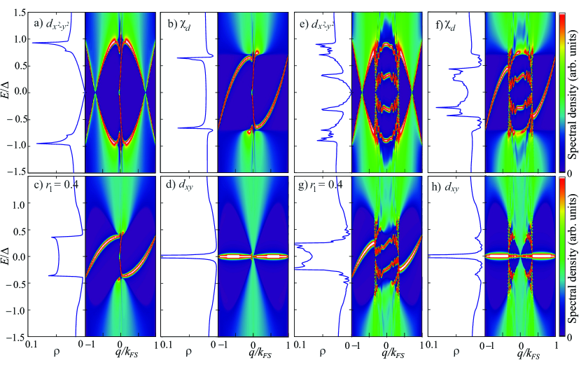
Figure 3: Spectral density and DOS of the graphene N-G-S junction at $x=0$. Results for $d$-wave superconductors with different values of the pairing phase. The Fermi energy of the graphene layer is $E_{F}\!=\!0\Delta$ for (a,b,c,d) and $E_{F}\!=\!10\Delta$ for (e,f,g,h). In all cases, $E_{FN}\!=\!E_{FS}\!=\!30\Delta$, $t_{L}\!=\!0.1$, $t_{R}\!=\!1$, and $d\!=\!2\xi$.

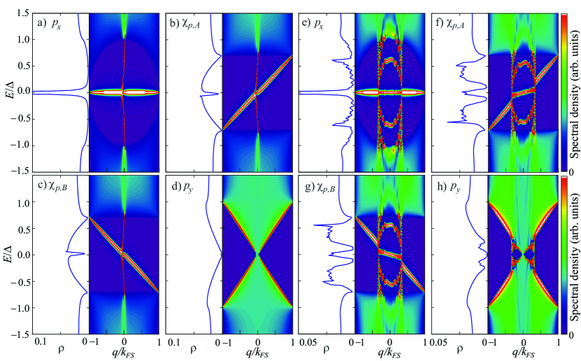
Figure 4: Spectral density and DOS of the graphene N-G-S junction at $x=0$. Results for different types of $p$-wave superconductors. The Fermi energy of the graphene layer is $E_{F}\!=\!0\Delta$ for (a,b,c,d) and $E_{F}\!=\!10\Delta$ for (e,f,g,h). In all cases, $E_{FN}\!=\!E_{FS}\!=\!30\Delta$, $t_{L}\!=\!0.1$, $t_{R}\!=\!1$, and $d\!=\!2\xi$.

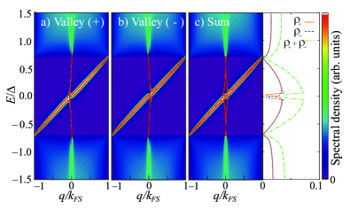
Figure 5: Valley dependence of the spectral density and DOS of the graphene N-G-S junction at $x=0$. All plots are calculated for the chiral $p$-wave symmetry.

IV Density of states of the N-G-S junction

We now focus on the N-G-S junction sketched in Fig. 1(a). The intermediate region is a graphene layer with zigzag edges along the $y$-direction. When uncoupled from the reservoirs, the isolated graphene layer features localized zigzag edge states (ZZES) at $E\!=-E_{F}$. The coupling to the leads, controlled by the interface transparencies $t_{L,R}$, splits the ZZES which completely vanish at perfect transparencyBrey and Fertig (2006); Tkachov (2007); Burset et al. (2009); Tkachov (2009); Tkachov and Hentschel (2009); Herrera et al. (2010). The ZZES have a resonant contribution to the density of states, with magnitude much bigger than that of any other resonances or Andreev states considered here. They thus play an important role in the tunneling properties, as shown in the next section. In what follows, we take $t_{L}\!=\!0.1$ and $t_{R}\!=\!1$. A perfect coupling to the superconductor ($t_{R}\!=\!1$) guarantees that at the interface there is no ZZES and only Andreev reflections take place. By considering the coupling to the N lead in the tunnel regime ($t_{L}\!=\!0.1$), we include an important contribution from normal backscattering processes and from the ZZES at that edge. We choose the width of the graphene layer to be $d\!=\!2\xi$, with $\xi\!=\!\hbar v_{F}/\Delta$ the superconducting coherence length. This is enough for Andreev processes to contribute to the conductance to the leftmost electrode, but it also reduces the effect of the ZZES on the density of states calculated close to the G-S interface. Additionally, the reduced N-G tunneling increases the finite-size effects at the intermediate region.

Under such conditions, we plot in Fig. 3 the spectral density and DOS, calculated, respectively, from Eq. (6) and Eq. (7) close to the G-S interface ($x\!\rightarrow\!0$), for the $d$-wave symmetries. An equivalent plot for $p$-wave symmetries is shown in Fig. 4. Before analyzing the effect of the different pairing symmetries, we first comment on some common effects stemming from the band structure of the finite graphene layer.

The asymmetry of the bands with respect to the wavevector is better explained in Fig. 5 using chiral $p$-wave symmetry. The results in Fig. 3 and Fig. 4 are calculated for one of the valleys. For the other valley, the pair potential is also given by Eq. (3) but with the change $q\!\rightarrow\!-q$. As a consequence, the asymmetric FPR bands inside the Dirac cone are reflected in the $q$-axis for the other valley. The symmetry with respect to the energy in the DOS is thus recovered when the contribution from both valleys is considered together, see Fig. 5(c). The change of valley does not affect the dispersion relation of the IBS and SABS for chiral symmetries, and chirality is preserved in the total contribution of the spectral density, as it is shown in Fig. 5.

The finite size is manifested by the appearance of discrete bands instead of a continuous spectrum like in Fig. 2. For the undoped cases with $E_{F}\!=\!0$, e.g., Fig. 3(a-d), a band appears inside the gap at the Dirac point. A second band can be perceived close to the gap edge, for the symmetries with a full gap around $q\!\sim\!0$, like $d_{x^{2}-y^{2}}$ in Fig. 3(a) and $p_{x}$ in Fig. 4(a). To better analyze the FPR, we consider a heavily-doped regime with $E_{F}\!=\!10\Delta$ in Fig. 3(e-h) and Fig. 4(e-h). The extra bands emerging from high doping appear as wavy arc-shaped bands framed by the anisotropic superconducting gap and no ZZES band is present as predicted by Eq. (20).

We now focus on the effect of proximity induced unconventional pairing in graphene. For the $d_{x^{2}-y^{2}}$-wave symmetry, graphene’s band structure is deformed according to the $\cos 2\theta$ dependence of the pairing amplitude, cf. Fig. 3(a). As a result, the DOS features a $V$-shaped gapped profile, even in the presence of FPR, see Fig. 3(e). Even after adding up all the momentum channels in the DOS, we can still observe in the left panel of Fig. 3(a) a small contribution from the layer’s second band as a small peak below the gap edge. For $d_{xy}$-wave symmetry, where the gap edge now follows a $\sin 2\theta$ dependence, there is a clear zero-energy peak in the DOS coming from the emergence of a flat band in the spectrum, see Fig. 3(d,h). The intermediate instance between these symmetries is well represented by $r_{1}\!=\!0.4$, Fig. 3(c,g), where the flat band acquires a dispersion at the same time that the gap edge is deformed similarly to the $d_{xy}$-wave case. The DOS captures such a superposition of $d$-wave states displaying a smaller gap with increased DOS but still featuring a minimum at zero energy. The FPR can now mask this effect in the DOS, cf. Fig. 3(g), but the local minimum at $E\!=\!0$ remains. The situation where both $d_{x^{2}-y^{2}}$ and $d_{xy}$ weight exactly the same in the pairing states is the chiral $d$-wave ($\chi_{d}$) case, shown in Fig. 3(b,f). For this chiral symmetry the effect of the SABS is better perceived: the DOS is finite but features a $U$-shaped gap profile with sharp edges and the SABS crossing the gap is clearly visible in the spectral density.

For $p$-wave symmetries, we find analogous results with some important differences. Similarly to the $d_{xy}$-wave case, $p_{x}$-wave symmetry features a zero-energy peak in the DOS from a flat band, independently of the doping level, see Fig. 4(a,e). Analogously, $p_{y}$-wave symmetry features a $V$-shaped DOS comparable to that of $d_{x^{2}-y^{2}}$-wave, as shown in Fig. 4(d,h). It is important to notice that for $p_{y}$-wave there are no resonances at $E\!=\!\pm\Delta$, a characteristic feature of $p$-wave superconductors. In the presence of disorder, $d_{xy}$ and $p_{x}$-wave (and, correspondingly, $d_{x^{2}-y^{2}}$ and $p_{y}$-wave) display different behavior and can be thus distinguished betterLu et al. (2016); Burset et al. (2017).

The chiral $p$-wave symmetry, $\chi_{p}$, shows an interesting difference with respect to the $\chi_{d}$ case. The $\chi_{p}$ SABS have a linear dispersion which results in a convex enhanced DOS below the gap. Interestingly, there is still a minimum at $E\!=\!0$, stemming from graphene’s band structure. Indeed, the convex enhanced DOS is suppressed around $|E|\!\sim\!0$ in Fig. 4(b,c) for the undoped case. For the doped situation, the linear chiral SABS has two different contributions. Outside graphene’s band, it mixes with the IBS and features a linear dispersion responsible for the enhanced DOS. Close to zero energy, however, the SABS mixes with a FPR resonance that always crosses zero at $\hbar q\!\sim\!0$. Additionally, the wavy FPR bands become small peaks in the DOS for subgap energies.

The doped case reveals an important difference between the $d$- and $p$-wave symmetries. Comparing Fig. 3(e,f,g) and Fig. 4(e,f,g), we immediately observe that, for the same set of system parameters, the $d$-wave symmetry cases, with the notable exception of $r_{1}\!=\!0$, feature an even number of FPR bands while the number is odd for $p$-wave symmetry. Additionally, one of the $p$-wave bands is always zero at $\hbar q\!\sim\!0$. This is a consequence of the different symmetry classification in two dimensions of the topologically trivial $d$-wave case, when $r_{1}\!\neq\!0$ in Eq. (3), and the nontrivial $p$-wave and $d_{xy}$-wave casesSchnyder et al. (2008); Sato (2009, 2010); Ryu et al. (2010); Budich and Trauzettel (2013); Kashiwaya et al. (2014).

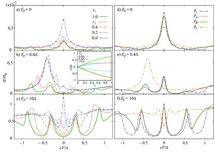
Figure 6: Differential conductance of the graphene N-G-S junction. (a,b,c) Conductance for $d$-wave superconductors with different values of the pairing phase. The inset in (b) shows the dependence of the first resonance on $r_{1}$ for different values of the Fermi energy of the graphene stripe. (d,e,f) Similar results for $p$-wave superconductors. The Fermi energy of the graphene layer is taken at $E_{F}\!=\!0$ (a,d), $E_{F}\!=\!0.4\Delta$ (b,e), and $E_{F}\!=\!10\Delta$ (c,f). In all cases, $E_{FN}\!=\!E_{FS}\!=\!30\Delta$, $t_{L}\!=\!0.1$, $t_{R}\!=\!1$, and $d\!=\!2\xi$.

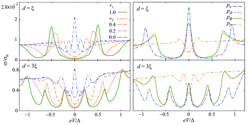
Figure 7: Differential conductance of the graphene N-G-S junction for different widths. (Left) Conductance for $d$-wave superconductors with different values of the pairing phase. (Right) Similar results for $p$-wave superconductors. The graphene layer’s width is $d\!=\!\xi$ (top) and $d\!=\!3\xi$ (bottom). In all cases, $E_{FN}\!=\!E_{FS}\!=\!30\Delta$, $E_{F}\!=\!10\Delta$, $t_{L}\!=\!0.1$, and $t_{R}\!=\!1$.

V Differential conductance

We now analyze the differential conductance in the N-G-S junction sketched in Fig. 1(a). To this end, we plot Eq. (14) in Fig. 6 for $d$-wave (left column) and $p$-wave symmetries (right column). Results for $s$-wave are similar to those of $d_{x^{2}-y^{2}}$.

We start analyzing $s$- and $d$-wave symmetries. In Fig. 6(a), we plot the conductance at $E_{F}\!=\!0$ for different values of $r_{1}$, see Fig. 1(c). In all cases, there is a strong zero-bias conductance peak (ZBCP). When $r_{1}\!\neq\!0$, we also observe two small peaks at the position of the effective superconducting gap. The ZBCP in this setup is mostly due to the contribution of graphene’s ZZES at the N-G interface, where $t_{L}\!=\!0.1$. However, for the case with $r_{1}\!=\!0$ where the superconductor features a nodal, flat band, the ZBCP is greatly enhanced since now merges the SABS with the ZZES. This is a signature of the gap closing and edge state for $d_{xy}$-wave pairing. As $r_{1}$ increases from zero, and the $d_{xy}$-wave mixes with the $d_{x^{2}-y^{2}}$-wave, this zero-energy state splits giving rise to the effective gap edge, cf. Fig. 3(a). We show the evolution of the split conductance peaks from finite $r_{1}$ in the inset of Fig. 6(b).

By setting $E_{F}\!\neq\!0$, as it is done in Fig. 6(b,c), the ZZES moves away from zero voltage. In these doped cases, a ZBCP only appears for $d_{xy}$-wave symmetry ($r_{1}\!=\!0$). As we increase the doping of the central graphene region, the FPR become more pronounced, see Fig. 6(b,c). The main reason is that the Andreev processes at the G-S interface become retro-reflections for $E_{F}\!>\!\Delta$, which favors the formation of closed trajectories in the G region. The geometric origin of the FPR is more clearly shown in Fig. 7, where we plot the conductance with the same parameters as in Fig. 6(c) but with $L\!=\!\xi$ (top) and $L\!=\!3\xi$ (bottom).

We now consider $p$-wave pairing symmetries. As in the previous section, we only consider $p_{x}$-, $p_{y}$-, and chiral $p$-wave symmetries. For the undoped graphene layer with $E_{F}\!=\!0$, shown in Fig. 6(d), the conductance features a clear ZBCP. For $p_{y}$-wave pairing, the ZBCP is mostly due to the ZZES and has the smallest value because of the absence of any SABS band, cf. Fig. 4(d). For the other symmetries, both the ZZES and the SABS contribute to the ZBCP. The highest value of the peak corresponds to $p_{x}$-wave state, where the SABS-IBS is a flat nodal surface state, as it is shown in Fig. 4(a).

Setting $E_{F}\!\neq\!0$ in Fig. 6(e,f), we clearly see that the ZBCP survives for all symmetries except for the trivial $p_{y}$-wave. In the strongly doped case with $E_{F}\!=\!10\Delta$, the ZBCP coexists with the FPRs for the nontrivial cases. Comparing Fig. 6(c) and Fig. 6(f), calculated with $L\!=\!2\xi$, it is clear that the $d$-wave cases (with $r_{1}\!\neq\!0$) feature an even number of peaks, while the $p_{x}$- and chiral $p$-wave cases have the additional ZBCP. The number of resonances is determined by the length of the graphene layer as shown in Fig. 7.

It is interesting to note that the magnitude of the ZZES peak at $eV\!=\!-E_{F}$ in relation to the ZBCP seems to follow the opossite behavior for $p$- and $d$-wave cases, cf. Fig. 6(b) and Fig. 6(e). The ZZES peak in Fig. 6(e) is rather small for the nontrivial $p_{x}$- and chiral $p$-wave states, but has a quite pronounced contribution in the $p_{y}$-wave case. In contrast, a strong ZZES peak appears when nontrivial $d_{xy}$-wave symmetry becomes dominant but it is weak for the $d_{x^{2}-y^{2}}$-wave dominated cases. The magnitude of the ZZES peak is completely determined by the ratio between the real and imaginary parts of the pairing as defined in Eq. (3). When the real part dominates, i.e., for $r_{1}\!\rightarrow\!1$ ($p_{x}$- and $d_{x^{2}-y^{2}}$-waves), the effective gap edge $\Delta_{\text{eff}}$ is maximum around $\hbar q\!\sim\!0$ ($\Delta_{\text{eff}}\approx\left|\Delta\left(\theta=0\right)\right|$). On the contrary, when the imaginary part becomes dominant for $r_{1}\!\rightarrow\!0$ ($p_{y}$- and $d_{xy}$-waves), the effective gap edge around $\hbar q\!\sim\!0$ is reduced, merging with the ZZES when $E_{F}\!\lesssim\!\Delta_{\mathrm{eff}}$. The dependence of the effective gap with $\hbar q$ for the different pairings is clearly observed in Fig. 3(a,d) and Fig. 4(a,d). The ZZES appears for values of $\hbar q$ that are close to zero for $d_{xy}$- and $p_{y}$-wave ($r_{1}\!\rightarrow\!0$) and far away from zero for $d_{x^{2}-y^{2}}$- and $p_{x}$-wave ($r_{1}\!\rightarrow\!1$). After averaging over the incident modes, the ZZES thus provides a stronger contribution around $|\hbar q|\!\sim\!0$ for pairings with $r_{1}\!\rightarrow\!0$, resulting in the strong peaks at $eV\!=\!-E_{F}$ in Fig. 6(b) and Fig. 6(e).

Finally, for the strongly doped case in Fig. 6(f) we clearly observe some of the characteristic behaviors of $p$-wave superconductors. Chiral $p$- and $p_{x}$-wave states feature a clear ZBCP due to the ZES bands showed in Fig. 4(f,g). The $p_{y}$-wave pairing displays a $V$-shape gap, with a finite minimum even though the conductance is calculated in the tunnel limit.

VI Conclusion

Motivated by recent experimental advances in the implementation of graphene–superconductor ballistic junctionsCalado et al. (2015); Ben Shalom et al. (2016); Efetov et al. (2016), we have theoretically studied the transport properties of a ballistic, finite-size graphene layer contacted by a normal and a superconducting lead. We particularly considered the emergence of unconventional superconductivity in the graphene layerDi Bernardo et al. (2017); Cao et al. (2018).

Using a microscopic description based on Green’s functions techniques, we included in our model several experimentally relevant issues like the Fabry-Pérot resonances originated by the finite length of the graphene layer, the different transmission of the graphene-reservoir interfaces, and the presence of graphene’s edge states. We calculated the spectral density, DOS and differential conductance of the graphene junction in the presence of unconventional superconductivity with different forms of $d$- or $p$-wave symmetry. We find that for energies below the gap, both the DOS and conductance show a very intricate profile due to the presence of several types of resonances. In addition to the Fabry-Pérot resonances and graphene’s edge states, we identify the emergence of Andreev surface states and interface bound states with different dispersions. Our analytical results allows us to identify the separate contribution from each state to the DOS and their impact on the differential conductance. We thus determine the optimal conditions for the detection of unconventional superconductivity using graphene layers.

In particular, we find that the presence of graphene’s zigzag edge states can mask the emergence of a ZBCP if the superconducting pairing allows for one. A finite doping is enough to separate and distinguish the contributions from ZZES and SABS to the conductance. In the presence of high doping compared to the superconducting gap, the geometrical FPRs become stronger. However, the subgap SABS from the induced unconventional pairing still have clear signatures in the spectral density and the DOS. Such resonances do not hide the ZBCP originating from $d_{xy}$-, $p_{x}$- or chiral $p$-wave states, for lengths of the graphene layer comparable to the superconducting coherence length. Additionally, these nontrivial pairings always display an odd number of conductance resonances. Even in the presence of high doping, the FPRs mix with the SABS but the topological zero energy states are still present in the spectral density and result in additional zero bias peaks in the conductance.

Our results provide a useful guide for future experiments that combine graphene with unconventional superconductors or that study emerging unconventional superconductivity in graphene induced by the asymmetry of the hexagonal lattice.

Appendix A Boguliubov-de Gennes-Dirac Hamiltonian.

We consider a semi-infinite graphene layer with a zigzag edge along the $y$-axis at $x_{L}\!=\!0$ and extending into the $x\!>\!0$ half-plane. With this orientation the Brillouin zone has Dirac points (valleys) at $\mathbf{K}_{\pm}=(0,\pm K)$. The conserved momentum along the $y$ direction is $\hbar q$. The wave function for the sublattice $A(B)$ is then given by

$$\Psi_{A(B)}\left(\mathbf{r}\right)=\mathrm{e}^{iKy}\Phi_{A(B)}^{+}\left(\mathbf{r}\right)+\mathrm{e}^{-iKy}\Phi_{A(B)}^{-}\left(\mathbf{r}\right),$$

where the functions $\Phi_{A(B)}^{\pm}\left(\mathbf{r}\right)$ are solutions of a 2D Dirac equation

$$\hat{H}_{\pm}={} \hat{p}_{x}\sigma_{x}\pm q\sigma_{y},$$

$$0={} \left(\hat{H}_{\pm}-\left(E_{F}+E\right)\right)\Phi^{\pm}\left(\mathbf{r}\right),$$

$$\Phi^{\pm}\left(\mathbf{r}\right)={} \left(\begin{array}[]{cc}\Phi_{A}^{\pm}\left(\mathbf{r}\right)&\Phi_{B}^{\pm}\left(\mathbf{r}\right)\end{array}\right)^{T}$$

$$={} \left(\begin{array}[]{cc}f_{A}^{\pm}\left(x\right)&f_{B}^{\pm}\left(x\right)\end{array}\right)^{T}\mathrm{e}^{iqy}.$$

Zigzag edges are formed by a line of atoms of only one of graphene’s sublattices (A or B) and do not mix valleys. If we adopt a Dirichlet boundary condition, we get

$$\Psi_{A(B)}\left(\mathbf{r}\right)={} \mathrm{e}^{iKy}\Phi_{A(B)}^{+}\left(x_{L},y\right)+\mathrm{e}^{-iKy}\Phi_{A(B)}^{-}\left(x_{L},y\right)=0,$$

$$\Rightarrow f_{A(B)}^{\pm}\left(x_{L}\right)=0.$$

Then, we can consider the boundary problem separately and use only one valley. The Dirac-Bogoliubov-de Gennes (DBdG) Hamiltonian for a 2D graphene sheet adopts the form

$$H_{BDG}=\left(\begin{array}[]{cc}\check{H}-E_{F}\check{I}&\check{\Delta}(\mathbf{k})\check{I}\\ \check{\Delta}^{{\dagger}}(\mathbf{k})\check{I}&E_{F}\check{I}-T\check{H}T^{-1}\end{array}\right),$$

where we are considering the weak-coupling approximation ($\mathbf{k}$ fixed on the Fermi surface) where the order parameter is only angle dependentLinder and Sudbø (2008), i.e.,

$$\check{\Delta}(\mathbf{k})=\check{\Delta}(\theta)\text{,}$$

and $\check{H}$ is the single-particle Hamiltonian in sublattice and valley spaces

$$\check{H}=\left(\begin{array}[]{cc}\hat{H}_{+}&0\\ 0&\hat{H}_{-}\end{array}\right).$$

Valley degeneracy allows us to consider only one of the two valley sets. Then, by using that $\left[\check{H},T\right]\!=\!0$, the $8\times 8$ matrix decouples to a $4\times 4$ matrix equation for zigzag edges, namely,

$$H_{BDG}=\left(\begin{array}[]{cc}\hat{H}_{\pm}-E_{F}\sigma_{0}&\Delta(\mathbf{k})\sigma_{0}\\ \Delta^{{\dagger}}(\mathbf{k})\sigma_{0}&E_{F}\sigma_{0}-\hat{H}_{\pm}\end{array}\right).$$ (22)

We adopt for the pair potential the following anisotropic symmetries [see Fig. 1(c)]

$$\Delta(\theta_{\pm})={} \Delta_{1}\cos(n\theta_{\pm})+i\Delta_{2}\sin(n\theta_{\pm}),$$

$$n={} 0\text{ \ for }s\text{-wave,}$$

$$n={} 1\text{ \ for }p\text{-wave,}$$

$$n={} 2\text{ \ for }d\text{-wave,}$$

where the parameters $\Delta_{1}$ and $\Delta_{2}$ obey the relations

$$\Delta_{i}\equiv r_{i}\Delta_{0}\text{,}$$

$$\sqrt{r_{1}^{2}+r_{2}^{2}}= 1,$$

with $i\!=\!1,2$, and their respective phases are defined by

$$\varphi_{\pm}=-i\ln\left(\frac{\Delta\left(\theta_{\pm}\right)}{\left|\Delta\left(\theta_{\pm}\right)\right|}\right)\text{.}$$

Appendix B Green’s function of graphene layer with zigzag edges and induced unconventional superconductivity.

The solutions of the DBdG equations have the form

$$\psi_{\pm}^{e}={} \mathrm{e}^{\pm ik_{e}x}\left(u_{0}\phi_{e}^{\pm},v_{0}\mathrm{e}^{-i\varphi_{\pm}}\phi_{e}^{\pm}\right)^{T}\text{,}$$

$$\psi_{\pm}^{h}={} \mathrm{e}^{\pm ik_{h}x}\left(v_{0}\phi_{h}^{\pm},u_{0}\mathrm{e}^{-i\varphi_{\pm}}\phi_{h}^{\pm}\right)^{T}\text{,}$$

with

$$\phi_{e\left(h\right)}^{+}={} \left(1,\mathrm{e}^{i\alpha_{e\left(h\right)}}\right)^{T},\,\phi_{e\left(h\right)}^{-}=\left(1,-\mathrm{e}^{-i\alpha_{e\left(h\right)}}\right)^{T},$$

$$\mathrm{e}^{i\alpha_{e(h)}}={} \hbar v_{F}\frac{k_{e(h)}+iq}{E_{F}\pm E}\,,\quad\Omega=\sqrt{E^{2}-\left|\Delta\right|^{2}},$$

$$k_{e\left(h\right)}={} \operatorname{sgn}\left(E_{F}\pm\Omega\right)\sqrt{\frac{\left(E_{F}\pm\Omega\right)^{2}}{\hbar^{2}v_{F}^{2}}-q^{2}},$$

$$u_{0}={} \sqrt{\frac{1}{2}\left(1+\frac{\Omega}{E}\right)},\,v_{0}=\sqrt{\frac{1}{2}\left(1-\frac{\Omega}{E}\right)}.$$

The wavefunctions $\psi_{\pm}^{\varepsilon}$ propagate under a pair potential $\Delta$, while their conjugates, $\bar{\psi}_{\pm}^{\varepsilon}$, move under $\Delta^{\ast}$. Therefore the functions $\bar{\psi}_{\pm}^{\varepsilon}$ can be constructed from the solutions $\psi_{\pm}^{\varepsilon}$ by changing $\Delta$ by $\Delta^{\ast}$ and multiplying by the conjugation matrix $\hat{\sigma}_{z}$ (see more details in Ref. Herrera et al., 2010). For a semi-infinite system with one edge, the asymptotic solutions of the DBdG equations are a superposition of normal reflection and Andreev reflections as follows

$$\psi_{<}^{e}= \psi_{-}^{e}+r_{e}\psi_{+}^{e}+r_{h}\psi_{-}^{h}\text{,}$$

$$\psi_{<}^{h}= \psi_{+}^{h}+r_{h}^{\prime}\psi_{-}^{h}+r_{e}^{\prime}\psi_{+}^{e}\text{,}$$

$$\psi_{>}^{e}= \psi_{+}^{e}\text{,}$$

$$\psi_{>}^{h}= \psi_{-}^{h}\text{,}$$

where $r_{e(h)}$ are the reflection coefficients. As a boundary condition we adopted a zigzag border of atoms of sublattice B, so that the B component must be zero at $x\!=\!0$. It then follows that

$$r_{e}= \mathrm{e}^{-2i\alpha_{e}}\frac{\left(1-\Gamma_{0}^{2}\right)}{1-\Gamma_{0}^{2}\mathrm{e}^{-i\Delta\varphi}}=r_{h}^{\prime}\mathrm{e}^{i\Delta\varphi}\mathrm{e}^{-2i\alpha_{h}}\mathrm{e}^{-2i\alpha_{e}},$$

$$r_{h}= \frac{\Gamma_{0}\left(\mathrm{e}^{-i\Delta\varphi}-1\right)}{1-\Gamma_{0}^{2}\mathrm{e}^{-i\Delta\varphi}}\left(\mathrm{e}^{i\alpha_{h}}\mathrm{e}^{-i\alpha_{e}}\right)=r_{e}^{\prime},$$

$$\Gamma_{0}= \frac{v_{0}}{u_{0}}.$$

From the asymptotic solutions that obey specific boundary conditions at the left ($<$) and right ($>$) edges of a ribbon, we construct the Green’s function asMcMillan (1968); Furusaki and Tsukada (1991); Kashiwaya and Tanaka (2000); Herrera et al. (2010); Burset et al. (2015); Crépin et al. (2015); Breunig et al. (2018)

$$\check{g}_{q}(x,x^{\prime})=\left\{\!\begin{array}[]{cc}\sum\limits_{\mu,\nu}\check{C}_{\mu\nu}\psi_{<}^{\mu}\left(q,x\right)\bar{\psi}_{>}^{\nu T}\left(q,x^{\prime}\right)\check{\gamma},&x>x^{\prime}\\ \sum\limits_{\mu,\nu}\check{C}_{\mu\nu}^{\prime}\psi_{>}^{\mu}\left(q,x\right)\bar{\psi}_{<}^{\nu T}\left(q,x^{\prime}\right)\check{\gamma},&x<x^{\prime}\end{array}\right.,$$ (23)

where $\mu,\nu\!=\!e,h$ label electron- and hole-like solutions of the DBdG equations and we include $\check{\gamma}\!=\!\hat{\tau}_{0}\hat{\sigma}_{z}$, with $\hat{\tau}_{0}$ the identity matrix in Nambu space, to ensure covarianceHerrera et al. (2010). By integrating Eq. (4) on the infinitesimal interval $(x^{\prime}-\epsilon,$ $x^{\prime}+\epsilon)$, with $\epsilon\!\ll\!1$, we obtain the continuity relation

$$\lim_{\epsilon\rightarrow 0}\left[\check{g}_{q}\left(x^{\prime}+\epsilon,x^{\prime}\right)-\check{g}_{q}\left(x^{\prime}-\epsilon,x^{\prime}\right)\right]=-\frac{i}{\hbar v_{F}}\hat{\tau}_{z}\hat{\sigma}_{x},$$ (24)

with the Pauli matrix $\hat{\tau}_{z}$ acting in Nambu space. From Eq. (24) it is possible to determine the coefficients $\check{C}_{\mu\nu}^{(\prime)}$.

From the continuity relation we deduce the matrix coefficients

$$\check{C}_{eh\left(he\right)}^{\left(\prime\right)}={} 0,$$

$$\check{C}_{ee}={} \check{C}_{ee}^{\prime}=\check{C}_{hh}=\check{C}_{hh}^{\prime}=\frac{i}{\hbar v_{F}}\frac{1}{FH-AB}\check{Y},$$

$$\check{Y}={} \left(\begin{array}[]{cccc}-B&0&H&0\\ 0&-B&0&F\mathrm{e}^{i\varphi_{-}}\mathrm{e}^{i\varphi_{+}}\\ -F&0&A&0\\ 0&-H\mathrm{e}^{-i\varphi_{+}}\mathrm{e}^{-i\varphi_{-}}&0&A\end{array}\right),$$

$$A={} \Gamma_{0}^{2}\left(\mathrm{e}^{i\alpha_{h}}+\mathrm{e}^{-i\alpha_{h}}\right)-\left(\mathrm{e}^{i\alpha_{e}}+\mathrm{e}^{-i\alpha_{e}}\right),$$

$$B={} \left(\mathrm{e}^{-i\alpha_{h}}+\mathrm{e}^{i\alpha_{h}}\right)-\Gamma_{0}^{2}\left(\mathrm{e}^{i\alpha_{e}}+\mathrm{e}^{-i\alpha_{e}}\right),$$

$$H={} \Gamma_{0}\left[\mathrm{e}^{-i\varphi_{-}}\left(\mathrm{e}^{-i\alpha_{h}}-\mathrm{e}^{-i\alpha_{e}}\right)\right.$$

$$\left.+\mathrm{e}^{-i\varphi_{+}}\left(\mathrm{e}^{i\alpha_{h}}-\mathrm{e}^{i\alpha_{e}}\right)\right]\mathrm{e}^{i\varphi_{-}}\mathrm{e}^{i\varphi_{+}},$$

$$F={} \Gamma_{0}\left[\mathrm{e}^{-i\varphi_{+}}\left(\mathrm{e}^{-i\alpha_{h}}-\mathrm{e}^{-i\alpha_{e}}\right)\right.$$

$$\left.+\mathrm{e}^{-i\varphi_{-}}\left(\mathrm{e}^{i\alpha_{h}}-\mathrm{e}^{i\alpha_{e}}\right)\right].$$

Thus, the Green function for $x<x^{\prime}$ is given by the expression

$$\check{g}_{R}(x,x^{\prime})={} \check{C}_{ee}\left[\psi_{-}^{e}\left(x\right)\bar{\psi}_{+}^{eT}\left(x^{\prime}\right)+r_{e}\psi_{+}^{e}\left(x\right)\bar{\psi}_{+}^{eT}\left(x^{\prime}\right)\right.$$

$$\left.+r_{h}\psi_{-}^{h}\left(x\right)\bar{\psi}_{+}^{eT}\left(x^{\prime}\right)+\psi_{+}^{h}\left(x\right)\bar{\psi}_{-}^{hT}\left(x^{\prime}\right)\right.$$

$$\left.+r_{h}^{\prime}\psi_{-}^{h}\left(x\right)\bar{\psi}_{-}^{hT}\left(x^{\prime}\right)+r_{e}^{\prime}\psi_{+}^{e}\left(x\right)\bar{\psi}_{-}^{hT}\left(x^{\prime}\right)\right].$$

where the $q$ dependence has been omited. A similar expression is obtained for $x\!>\!x^{\prime}$ by exchanging the signs of the subindexes and changing $e,h\rightarrow h,e$ in the superindexes. For the particular case with $\left(x,x^{\prime}\right)\!=\!\left(0^{+},0\right)$, the Green function is given by

$$\check{g}_{R}=\frac{i}{\hbar v_{F}}\left(\begin{array}[]{cccc}\frac{\Psi_{31}H-B\Psi_{11}}{FH-AB}&0&\frac{\Psi_{33}H-B\Psi_{13}}{FH-AB}&0\\ -1&0&0&0\\ \frac{A\Psi_{31}-F\Psi_{11}}{FH-AB}&0&\frac{A\Psi_{33}-F\Psi_{13}}{FH-AB}&0\\ 0&0&1&0\end{array}\right),$$ (25)

with

$$\Psi_{11}={} 1+\Gamma_{0}^{2}+2\Gamma_{0}r_{h}+r_{e}\left(\Gamma_{0}^{2}\mathrm{e}^{2i\alpha_{h}}\mathrm{e}^{2i\alpha_{e}}\mathrm{e}^{-i\Delta\varphi}+1\right),$$

$$\Psi_{31}={} \Gamma_{0}\left(\mathrm{e}^{-i\varphi_{-}}+\mathrm{e}^{-i\varphi_{+}}\right)+r_{h}\left(\mathrm{e}^{-i\varphi_{-}}+\Gamma_{0}^{2}\mathrm{e}^{-i\varphi_{+}}\right)$$

$$+\Gamma_{0}\mathrm{e}^{-i\varphi_{+}}r_{e}\left(\mathrm{e}^{2i\alpha_{h}}\mathrm{e}^{2i\alpha_{e}}+1\right),$$

$$\Psi_{13}={} \Gamma_{0}\left(\mathrm{e}^{i\varphi_{-}}+\mathrm{e}^{i\varphi_{+}}\right)+r_{h}\left(\mathrm{e}^{i\varphi_{+}}+\Gamma_{0}^{2}\mathrm{e}^{i\varphi_{-}}\right)$$

$$+\Gamma_{0}\mathrm{e}^{i\varphi_{-}}r_{e}\left(\mathrm{e}^{2i\alpha_{h}}\mathrm{e}^{2i\alpha_{e}}+1\right),$$

$$\Psi_{33}={} 1+\Gamma_{0}^{2}+2\Gamma_{0}r_{h}+r_{e}\left(\mathrm{e}^{2i\alpha_{h}}\mathrm{e}^{2i\alpha_{e}}+\Gamma_{0}^{2}\mathrm{e}^{-i\Delta\varphi}\right).$$

Following the same procedure, the Green function of a normal graphene stripe of length $d$ is given by

$$\check{g}_{0}(x,x^{\prime}>x)=\frac{-i}{\hbar v_{F}}\left(\begin{array}[]{cc}\hat{g}_{e}&0\\ 0&\hat{g}_{h}\end{array}\right),$$

with

$$\hat{g}_{e\left(h\right)}= \frac{\mathrm{e}^{\pm i\left(x^{\prime}-x\right)k_{e\left(h\right)}}}{D_{e\left(h\right)}}\left(\begin{array}[]{cc}IK&\mp s\mathrm{e}^{\pm i\alpha}IL\\ \mp s\mathrm{e}^{\mp i\alpha}JK&JL\end{array}\right)_{e(h)}\text{,}$$

$$D_{e\left(h\right)}= \left(\mathrm{e}^{-i\alpha_{e\left(h\right)}}+\mathrm{e}^{i\alpha_{e\left(h\right)}}\right)\left(1+\mathrm{e}^{\mp 2i\alpha_{e\left(h\right)}}\mathrm{e}^{\pm 2idk_{e\left(h\right)}}\right)\text{,}$$

$$I_{e\left(h\right)}= 1+\mathrm{e}^{\mp 2i\alpha_{e\left(h\right)}}\mathrm{e}^{\pm 2idk_{e\left(h\right)}}\mathrm{e}^{\pm 2ixk_{e\left(h\right)}}\text{,}$$

$$J_{e\left(h\right)}= 1-\mathrm{e}^{\pm 2idk_{e\left(h\right)}}\mathrm{e}^{\pm 2ixk_{e\left(h\right)}}\text{,}$$

$$K_{e\left(h\right)}= 1-\mathrm{e}^{\mp 2ix^{\prime}k_{e\left(h\right)}}\text{,}$$

$$L_{e\left(h\right)}= 1+\mathrm{e}^{\mp 2i\alpha_{e\left(h\right)}}\mathrm{e}^{\mp 2ix^{\prime}k_{e\left(h\right)}}\text{,}$$

and $s\!=\!1$. For $x\!>\!x^{\prime}$ the Green function is obtained from the transpose of the last expression by interchanging the coordinates ($x\!\leftrightarrow\!x^{\prime}$) and setting $s\!=\!-1$. For a semi-infinite graphene sheet, we have $D_{e\left(h\right)}\!=\!e^{-i\alpha_{e\left(h\right)}}+\mathrm{e}^{i\alpha_{e\left(h\right)}}$ and $F_{e\left(h\right)}\!=\!J_{e\left(h\right)}\!=\!1$. Since Green functions for graphene with zigzag edges depend on the order of the spatial arguments, the following convention was adopted for Dyson’s equation [Eq. (5)] thats couples two regions with edges at $x\!=\!0$, namely,

$$\check{G}_{ij}(x,x^{\prime})={} \check{g}_{ij}(x,x^{\prime})+\check{g}_{iR}(x,0^{-})\check{\Sigma}_{RL}\check{G}_{Lj}(-0^{+},x^{\prime})$$

$$={} \check{g}_{ij}(x,x^{\prime})+\check{g}_{iR}(x,-0^{-})\check{\Sigma}_{LR}\check{G}_{Rj}(0^{+},x^{\prime}),$$

where $0^{\pm}$ are positive infinitesimal real numbers satisfying $0^{-}\!<\!0^{+}$. For example for $\check{G}_{LL}$ we obtain

$$\check{G}_{LL}={} \check{g}_{LL}\left(I+\Sigma_{LR}M_{RR}\check{g}_{RR}\Sigma_{RL}\check{g}_{LL}\right)\text{,}$$

$$M_{RR}={} \left[I-\check{g}_{RR}\Sigma_{RL}\check{g}_{LL}\Sigma_{LR}\right]^{-1}\text{.}$$

For the model of a highly doped graphene superconductor electrode ($\mathrm{e}^{i\alpha_{e\left(h\right)}}\!=\!1$) coupled with $t\!=\!1$ to a graphene film of length $d$ the last Green function has the following denominator

$$D=\left(1-\mathrm{e}^{-i\Delta\varphi}\Gamma_{0}^{2}\right)^{2}X,$$ (26)

with

$$X={} 1+\frac{\Gamma_{0}^{2}+\mathrm{e}^{i\Delta\varphi/2}}{\Gamma_{0}^{2}-\mathrm{e}^{i\Delta\varphi/2}}\left(\mathrm{e}^{-i\alpha_{+}}h_{+}+\mathrm{e}^{i\alpha_{-}}h_{-}\right)$$

$$+\mathrm{e}^{-i\alpha_{+}}\mathrm{e}^{i\alpha_{-}}h_{+}h_{-}.$$

The first factor contains the SABS dispersion relation in Eq. (17), namely,

$$1-\mathrm{e}^{-i\Delta\varphi}\Gamma_{0}^{2}=\left(E^{2}-E_{SABS}^{2}\right)/\Lambda\text{,}$$

$$\Lambda=\frac{1}{2}\mathrm{e}^{i\Delta\varphi/2}\left(E+\Omega\right)\left(\Omega\cos\left(\Delta\varphi/2\right)-iE\sin\left(\Delta\varphi/2\right)\right),$$

where $\Lambda$ is responsible for some effects of superconducting phase chirality in the SABS. The factor $X$ encodes the IBS and FPR dispersion relations [Eq. (18)],

$$X\Lambda_{X}=\left(E^{2}-E_{IBS-FPR}^{2}\right)/\Lambda_{X},$$

$$\Lambda_{X}=\frac{E\left(\Phi-1\right)-\left(1+\Phi\right)\Omega}{\left(\mathrm{e}^{-i\alpha_{+}}h_{+}+\mathrm{e}^{i\alpha_{-}}h_{-}\right)\left(1-Z^{2}\right)}$$

$$\times\frac{E\left[C\left(\Phi-1\right)+\left(1+\Phi\right)\right]-\Omega\left[\left(1-\Phi\right)-C\left(1+\Phi\right)\right]}{\left(C\left(\Phi-1\right)+\left(1+\Phi\right)\right)^{2}}\text{,}$$

with $\Phi\!=\!\mathrm{e}^{-i\Delta\varphi}$. Here $\Lambda_{X}$ also includes some effects of valley and superconducting phase chirality.

References

- Sigrist and Ueda (1991) Manfred Sigrist and Kazuo Ueda, “Phenomenological theory of unconventional superconductivity,” Rev. Mod. Phys. 63, 239–311 (1991).
- Kashiwaya and Tanaka (2000) Satoshi Kashiwaya and Yukio Tanaka, “Tunnelling effects on surface bound states in unconventional superconductors,” Reports on Progress in Physics 63, 1641 (2000).
- Lee et al. (2006) Patrick A. Lee, Naoto Nagaosa, and Xiao-Gang Wen, “Doping a mott insulator: Physics of high-temperature superconductivity,” Rev. Mod. Phys. 78, 17–85 (2006).
- Mackenzie and Maeno (2003) Andrew Peter Mackenzie and Yoshiteru Maeno, “The superconductivity of and the physics of spin-triplet pairing,” Rev. Mod. Phys. 75, 657–712 (2003).
- Maeno et al. (2012) Yoshiteru Maeno, Shunichiro Kittaka, Takuji Nomura, Shingo Yonezawa, and Kenji Ishida, “Evaluation of spin-triplet superconductivity in sr2ruo4,” Journal of the Physical Society of Japan 81, 011009 (2012).
- Kallin (2012) Catherine Kallin, “Chiral p-wave order in sr 2 ruo 4,” Reports on Progress in Physics 75, 042501 (2012).
- Read and Green (2000) N. Read and Dmitry Green, “Paired states of fermions in two dimensions with breaking of parity and time-reversal symmetries and the fractional quantum hall effect,” Phys. Rev. B 61, 10267–10297 (2000).
- Ivanov (2001) D. A. Ivanov, “Non-abelian statistics of half-quantum vortices in -wave superconductors,” Phys. Rev. Lett. 86, 268–271 (2001).
- Alicea (2012) Jason Alicea, “New directions in the pursuit of majorana fermions in solid state systems,” Reports on Progress in Physics 75, 076501 (2012).
- Beenakker (2013) C.W.J. Beenakker, “Search for majorana fermions in superconductors,” Annual Review of Condensed Matter Physics 4, 113–136 (2013).
- Sarma et al. (2015) Sankar Das Sarma, Michael Freedman, and Chetan Nayak, “Majorana zero modes and topological quantum computation,” Npj Quantum Information 1, 15001 (2015).
- Lutchyn et al. (2010) Roman M. Lutchyn, Jay D. Sau, and S. Das Sarma, “Majorana fermions and a topological phase transition in semiconductor-superconductor heterostructures,” Phys. Rev. Lett. 105, 077001 (2010).
- Oreg et al. (2010) Yuval Oreg, Gil Refael, and Felix von Oppen, “Helical liquids and majorana bound states in quantum wires,” Phys. Rev. Lett. 105, 177002 (2010).
- Potter and Lee (2010) Andrew C. Potter and Patrick A. Lee, “Multichannel generalization of kitaev’s majorana end states and a practical route to realize them in thin films,” Phys. Rev. Lett. 105, 227003 (2010).
- Potter and Lee (2011) Andrew C. Potter and Patrick A. Lee, “Engineering a superconductor: Comparison of topological insulator and rashba spin-orbit-coupled materials,” Phys. Rev. B 83, 184520 (2011).
- Kallin and Berlinsky (2016) Catherine Kallin and John Berlinsky, “Chiral superconductors,” Reports on Progress in Physics 79, 054502 (2016).
- Nandkishore et al. (2012) Rahul Nandkishore, L. S. Levitov, and A. V. Chubukov, “Chiral superconductivity from repulsive interactions in doped graphene,” Nat Phys 8, 158–163 (2012).
- Black-Schaffer (2012) Annica M. Black-Schaffer, “Edge properties and majorana fermions in the proposed chiral -wave superconducting state of doped graphene,” Phys. Rev. Lett. 109, 197001 (2012).
- Black-Schaffer and Honerkamp (2014) Annica M Black-Schaffer and Carsten Honerkamp, “Chiral d -wave superconductivity in doped graphene,” Journal of Physics: Condensed Matter 26, 423201 (2014).
- Di Bernardo et al. (2017) A. Di Bernardo, O. Millo, M. Barbone, H. Alpern, Y. Kalcheim, U. Sassi, A. K. Ott, D. De Fazio, D. Yoon, M. Amado, A. C. Ferrari, J. Linder, and J. W. A. Robinson, “p-wave triggered superconductivity in single-layer graphene on an electron-doped oxide superconductor,” Nature Communications 8, 14024 (2017).
- Blonder et al. (1982) G. E. Blonder, M. Tinkham, and T. M. Klapwijk, “Transition from metallic to tunneling regimes in superconducting microconstrictions: Excess current, charge imbalance, and supercurrent conversion,” Phys. Rev. B 25, 4515–4532 (1982).
- Klapwijk and Ryabchun (2014) T. Klapwijk and S. Ryabchun, “Direct observation of ballistic andreev reflection.” Journal of Experimental and Theoretical Physics 119, 997–1017 (2014).
- Tanaka and Kashiwaya (1995) Yukio Tanaka and Satoshi Kashiwaya, “Theory of tunneling spectroscopy of -wave superconductors,” Phys. Rev. Lett. 74, 3451–3454 (1995).
- Kashiwaya et al. (1995) Satoshi Kashiwaya, Yukio Tanaka, Masao Koyanagi, Hiroshi Takashima, and Koji Kajimura, “Origin of zero-bias conductance peaks in high- superconductors,” Phys. Rev. B 51, 1350–1353 (1995).
- Kashiwaya et al. (1996) Satoshi Kashiwaya, Yukio Tanaka, Masao Koyanagi, and Koji Kajimura, “Theory for tunneling spectroscopy of anisotropic superconductors,” Phys. Rev. B 53, 2667–2676 (1996).
- Honerkamp and Sigristt (1998) Carsten Honerkamp and Manfred Sigristt, “Andreev reflection in unitary and non-unitary triplet states,” Journal of Low Temperature Physics 111, 895–915 (1998).
- Lu et al. (2016) Bo Lu, Pablo Burset, Yasunari Tanuma, Alexander A. Golubov, Yasuhiro Asano, and Yukio Tanaka, “Influence of the impurity scattering on charge transport in unconventional superconductor junctions,” Phys. Rev. B 94, 014504 (2016).
- Burset et al. (2017) Pablo Burset, Bo Lu, Shun Tamura, and Yukio Tanaka, “Current fluctuations in unconventional superconductor junctions with impurity scattering,” Phys. Rev. B 95, 224502 (2017).
- Wiedenmann et al. (2017) Jonas Wiedenmann, Eva Liebhaber, Johannes Kübert, Erwann Bocquillon, Pablo Burset, Christopher Ames, Hartmut Buhmann, Teun M. Klapwijk, and Laurens W. Molenkamp, “Transport spectroscopy of induced superconductivity in the three-dimensional topological insulator hgte,” Phys. Rev. B 96, 165302 (2017).
- Liang et al. (2001) Wenjie Liang, Marc Bockrath, Dolores Bozovic, Jason H. Hafner, M. Tinkham, and Hongkun Park, “Fabry - perot interference in a nanotube electron waveguide,” Nature 411, 665–669 (2001).
- Kretinin et al. (2010) Andrey V. Kretinin, Ronit Popovitz-Biro, Diana Mahalu, and Hadas Shtrikman, “Multimode fabry-pérot conductance oscillations in suspended stacking-faults-free inas nanowires,” Nano Letters 10, 3439–3445 (2010), pMID: 20695446, http://dx.doi.org/10.1021/nl101522j .
- Das Sarma et al. (2011) S. Das Sarma, Shaffique Adam, E. H. Hwang, and Enrico Rossi, “Electronic transport in two-dimensional graphene,” Rev. Mod. Phys. 83, 407–470 (2011).
- Rozhkov et al. (2011) A.V. Rozhkov, G. Giavaras, Yury P. Bliokh, Valentin Freilikher, and Franco Nori, “Electronic properties of mesoscopic graphene structures: Charge confinement and control of spin and charge transport,” Physics Reports 503, 77 – 114 (2011).
- Wehling et al. (2014) T.O. Wehling, A.M. Black-Schaffer, and A.V. Balatsky, “Dirac materials,” Advances in Physics 63, 1–76 (2014), http://dx.doi.org/10.1080/00018732.2014.927109 .
- Xia et al. (2011) Fengnian Xia, Vasili Perebeinos, Yu-ming Lin, Yanqing Wu, and Phaedon Avouris, “The origins and limits of metal-graphene junction resistance,” Nat Nano 6, 179 – 184 (2011).
- Wu et al. (2012) Yanqing Wu, Vasili Perebeinos, Yu-ming Lin, Tony Low, Fengnian Xia, and Phaedon Avouris, “Quantum behavior of graphene transistors near the scaling limit,” Nano Letters 12, 1417–1423 (2012), pMID: 22316333, http://dx.doi.org/10.1021/nl204088b .
- Drost et al. (2014) Robert Drost, Andreas Uppstu, Fabian Schulz, Sampsa K. Hämäläinen, Mikko Ervasti, Ari Harju, and Peter Liljeroth, “Electronic states at the graphene–hexagonal boron nitride zigzag interface,” Nano Letters 14, 5128–5132 (2014), pMID: 25078791.
- Drost et al. (2015) Robert Drost, Shawulienu Kezilebieke, Mikko M. Ervasti, Sampsa K. Hämäläinen, Fabian Schulz, Ari Harju, and Peter Liljeroth, “Synthesis of extended atomically perfect zigzag graphene - boron nitride interfaces,” Scientific Reports 5, 16741 (2015).
- Heersche et al. (2007) Hubert B. Heersche, Pablo Jarillo-Herrero, Jeroen B. Oostinga, Lieven M. K. Vandersypen, and Alberto F. Morpurgo, “Bipolar supercurrent in graphene,” Nature (London) 446, 56 (2007).
- Miao et al. (2007) F. Miao, S. Wijeratne, Y. Zhang, U. C. Coskun, W. Bao, and C. N. Lau, “Phase-coherent transport in graphene quantum billiards,” Science 317, 1530–1533 (2007).
- Shailos et al. (2007) A. Shailos, W. Nativel, A. Kasumov, C. Collet, M. Ferrier, S. Guéron, R. Deblock, and H. Bouchiat, “Proximity effect and multiple andreev reflections in few-layer graphene,” EPL (Europhysics Letters) 79, 57008 (2007).
- Du et al. (2008) Xu Du, Ivan Skachko, and Eva Y. Andrei, “Josephson current and multiple andreev reflections in graphene sns junctions,” Phys. Rev. B 77, 184507 (2008).
- Rickhaus et al. (2012) Peter Rickhaus, Markus Weiss, Laurent Marot, and Christian Schönenberger, “Quantum hall effect in graphene with superconducting electrodes,” Nano Letters 12, 1942–1945 (2012), pMID: 22417183.
- Calado et al. (2015) V. E. Calado, S. Goswami, G. Nanda, M. Diez, A. R. Akhmerov, K. Watanabe, T. Taniguchi, T. M. Klapwijk, and L. M. K. Vandersypen, “Ballistic josephson junctions in edge-contacted graphene,” Nat Nano 10, 761–764 (2015).
- Ben Shalom et al. (2016) M. Ben Shalom, M. J. Zhu, V. I. Fal[rsquor]ko, A. Mishchenko, A. V. Kretinin, K. S. Novoselov, C. R. Woods, K. Watanabe, T. Taniguchi, A. K. Geim, and J. R. Prance, “Quantum oscillations of the critical current and high-field superconducting proximity in ballistic graphene,” Nat Phys 12, 318–322 (2016).
- Efetov et al. (2016) D. K. Efetov, L. Wang, C. Handschin, K. B. Efetov, J. Shuang, R. Cava, T. Taniguchi, K. Watanabe, J. Hone, C. R. Dean, and P. Kim, “Specular interband andreev reflections at van der waals interfaces between graphene and nbse2,” Nat Phys 12, 328–332 (2016).
- Beenakker (2006) C. W. J. Beenakker, “Specular andreev reflection in graphene,” Phys. Rev. Lett. 97, 067007 (2006).
- Dirks et al. (2011) Travis Dirks, Taylor L. Hughes, Siddhartha Lal, Bruno Uchoa, Yung-Fu Chen, Cesar Chialvo, Paul M. Goldbart, and Nadya Mason, “Transport through andreev bound states in a graphene quantum dot,” Nature Physics 7, 386–390 (2011).
- Tan et al. (2015) Z. B. Tan, D. Cox, T. Nieminen, P. Lähteenmäki, D. Golubev, G. B. Lesovik, and P. J. Hakonen, “Cooper pair splitting by means of graphene quantum dots,” Phys. Rev. Lett. 114, 096602 (2015).
- Tonnoir et al. (2013) C. Tonnoir, A. Kimouche, J. Coraux, L. Magaud, B. Delsol, B. Gilles, and C. Chapelier, “Induced superconductivity in graphene grown on rhenium,” Phys. Rev. Lett. 111, 246805 (2013).
- Ludbrook et al. (2015) B. M. Ludbrook, G. Levy, P. Nigge, M. Zonno, M. Schneider, D. J. Dvorak, C. N. Veenstra, S. Zhdanovich, D. Wong, P. Dosanjh, C. Straßer, A. Stöhr, S. Forti, C. R. Ast, U. Starke, and A. Damascelli, “Evidence for superconductivity in li-decorated monolayer graphene,” Proc. Natl Acad. Sci. USA 112, 11795 (2015).
- Chapman et al. (2016) J. Chapman, Y. Su, C. A. Howard, D. Kundys, A. N. Grigorenko, F. Guinea, A. K. Geim, I. V. Grigorieva, and R. R. Nair, “Superconductivity in ca-doped graphene laminates,” Sci. Rep. 6, 23254 (2016).
- Uchoa and Castro Neto (2007) Bruno Uchoa and A. H. Castro Neto, “Superconducting states of pure and doped graphene,” Phys. Rev. Lett. 98, 146801 (2007).
- Jiang et al. (2008) Yongjin Jiang, Dao-Xin Yao, Erica W. Carlson, Han-Dong Chen, and JiangPing Hu, “Andreev conductance in the -wave superconducting states of graphene,” Phys. Rev. B 77, 235420 (2008).
- Cao et al. (2018) Yuan Cao, Valla Fatemi, Shiang Fang, Kenji Watanabe, Takashi Taniguchi, Efthimios Kaxiras, and Pablo Jarillo-Herrero, “Unconventional superconductivity in magic-angle graphene superlattices,” Nature (2018).
- Bhattacharjee and Sengupta (2006) Subhro Bhattacharjee and K. Sengupta, “Tunneling conductance of graphene nis junctions,” Phys. Rev. Lett. 97, 217001 (2006).
- Akhmerov and Beenakker (2007) A. R. Akhmerov and C. W. J. Beenakker, “Pseudodiffusive conduction at the dirac point of a normal-superconductor junction in graphene,” Phys. Rev. B 75, 045426 (2007).
- Tkachov (2007) Grigory Tkachov, “Fine structure of the local pseudogap and fano effect for superconducting electrons near a zigzag graphene edge,” Phys. Rev. B 76, 235409 (2007).
- Linder and Sudbø (2007) J. Linder and A. Sudbø, “Dirac fermions and conductance oscillations in - and -wave superconductor-graphene junctions,” Phys. Rev. Lett. 99, 147001 (2007).
- Linder and Sudbø (2008) Jacob Linder and Asle Sudbø, “Tunneling conductance in - and -wave superconductor-graphene junctions: Extended blonder-tinkham-klapwijk formalism,” Phys. Rev. B 77, 064507 (2008).
- Burset et al. (2008) P. Burset, A. Levy Yeyati, and A. Martín-Rodero, “Microscopic theory of the proximity effect in superconductor-graphene nanostructures,” Phys. Rev. B 77, 205425 (2008).
- Black-Schaffer and Doniach (2008) Annica M. Black-Schaffer and Sebastian Doniach, “Self-consistent solution for proximity effect and josephson current in ballistic graphene sns josephson junctions,” Phys. Rev. B 78, 024504 (2008).
- Burset et al. (2009) P. Burset, W. Herrera, and A. Levy Yeyati, “Proximity-induced interface bound states in superconductor-graphene junctions,” Phys. Rev. B 80, 041402 (2009).
- feng Sun and Xie (2009) Qing feng Sun and X C Xie, “Quantum transport through a graphene nanoribbon–superconductor junction,” Journal of Physics: Condensed Matter 21, 344204 (2009).
- Gómez et al. (2012) S. Gómez, P. Burset, W. J. Herrera, and A. Levy Yeyati, “Selective focusing of electrons and holes in a graphene-based superconducting lens,” Phys. Rev. B 85, 115411 (2012).
- Beenakker (2008) C. W. J. Beenakker, “Colloquium,” Rev. Mod. Phys. 80, 1337–1354 (2008).
- Burset et al. (2014) Pablo Burset, Felix Keidel, Yukio Tanaka, Naoto Nagaosa, and Björn Trauzettel, “Transport signatures of superconducting hybrids with mixed singlet and chiral triplet states,” Phys. Rev. B 90, 085438 (2014).
- Black-Schaffer and Doniach (2007) Annica M. Black-Schaffer and Sebastian Doniach, “Resonating valence bonds and mean-field -wave superconductivity in graphite,” Phys. Rev. B 75, 134512 (2007).
- McMillan (1968) W. L. McMillan, “Theory of superconductor-normal metal interfaces,” Phys. Rev. 175, 559–568 (1968).
- Furusaki and Tsukada (1991) Akira Furusaki and Masaru Tsukada, “Dc josephson effect and andreev reflection,” Solid State Communications 78, 299 – 302 (1991).
- Herrera et al. (2010) William J. Herrera, Pablo Burset, and A. Levy Yeyati, “A green function approach to graphene–superconductor junctions with well-defined edges,” Journal of Physics: Condensed Matter 22, 275304 (2010).
- Burset et al. (2015) Pablo Burset, Bo Lu, Grigory Tkachov, Yukio Tanaka, Ewelina M. Hankiewicz, and Björn Trauzettel, “Superconducting proximity effect in three-dimensional topological insulators in the presence of a magnetic field,” Phys. Rev. B 92, 205424 (2015).
- Crépin et al. (2015) François Crépin, Pablo Burset, and Björn Trauzettel, “Odd-frequency triplet superconductivity at the helical edge of a topological insulator,” Phys. Rev. B 92, 100507 (2015).
- Breunig et al. (2018) Daniel Breunig, Pablo Burset, and Björn Trauzettel, “Creation of spin-triplet cooper pairs in the absence of magnetic ordering,” Phys. Rev. Lett. 120, 037701 (2018).
- Gomez (2011) S. Gomez, “Transporte eléctrico en superconductores no convencionales,” (2011), www.bdigital.unal.edu.co/8020/.
- Cuevas et al. (1996) J. C. Cuevas, A. Martín-Rodero, and A. Levy Yeyati, “Hamiltonian approach to the transport properties of superconducting quantum point contacts,” Phys. Rev. B 54, 7366–7379 (1996).
- Löfwander et al. (2001) T Löfwander, V S Shumeiko, and G Wendin, “Andreev bound states in high- superconducting junctions,” Superconductor Science and Technology 14, R53 (2001).
- Brey and Fertig (2006) L. Brey and H. A. Fertig, “Electronic states of graphene nanoribbons studied with the dirac equation,” Phys. Rev. B 73, 235411 (2006).
- Tkachov (2009) Grigory Tkachov, “Dirac fermion quantization on graphene edges: Isospin-orbit coupling, zero modes, and spontaneous valley polarization,” Phys. Rev. B 79, 045429 (2009).
- Tkachov and Hentschel (2009) Grigory Tkachov and Martina Hentschel, “Coupling between chirality and pseudospin of dirac fermions: Non-analytical particle-hole asymmetry and a proposal for a tunneling device,” Phys. Rev. B 79, 195422 (2009).
- Schnyder et al. (2008) Andreas P. Schnyder, Shinsei Ryu, Akira Furusaki, and Andreas W. W. Ludwig, “Classification of topological insulators and superconductors in three spatial dimensions,” Phys. Rev. B 78, 195125 (2008).
- Sato (2009) Masatoshi Sato, “Topological properties of spin-triplet superconductors and fermi surface topology in the normal state,” Phys. Rev. B 79, 214526 (2009).
- Sato (2010) Masatoshi Sato, “Topological odd-parity superconductors,” Phys. Rev. B 81, 220504 (2010).
- Ryu et al. (2010) Shinsei Ryu, Andreas P Schnyder, Akira Furusaki, and Andreas W W Ludwig, “Topological insulators and superconductors: tenfold way and dimensional hierarchy,” New Journal of Physics 12, 065010 (2010).
- Budich and Trauzettel (2013) Jan Carl Budich and Björn Trauzettel, “From the adiabatic theorem of quantum mechanics to topological states of matter,” physica status solidi (RRL) – Rapid Research Letters 7, 109–129 (2013).
- Kashiwaya et al. (2014) Satoshi Kashiwaya, Hiromi Kashiwaya, Kohta Saitoh, Yasunori Mawatari, and Yukio Tanaka, “Tunneling spectroscopy of topological superconductors,” Physica E: Low-dimensional Systems and Nanostructures 55, 25 – 29 (2014).