A Coloring Book Approach to Finding Coordination Sequences

Abstract

An elementary method is described for finding the coordination sequences for a tiling, based on coloring the underlying graph. The first application is to the two kinds of vertices (tetravalent and trivalent) in the Cairo (or dual-$3^{2}\!.4.3.4$) tiling. The coordination sequence for a tetravalent vertex turns out, surprisingly, to be $1,4,8,12,16,\ldots$, the same as for a vertex in the familiar square (or $4^{4}$) tiling. The authors thought that such a simple fact should have a simple proof, and this article is the result. The method is also used to obtain coordination sequences for the $3^{2}\!.4.3.4$, $3.4.6.4$, $4.8^{2}$, $3.12^{2}$, and $3^{4}\!.6$ uniform tilings, and the snub-$632$ tiling. In several cases the results provide proofs for previously conjectured formulas.

This article presents a simple method for finding formulas for coordination sequences, based on coloring the underlying graph according to certain rules. It is illustrated by applying it to several uniform tilings and their duals.

1 Introduction

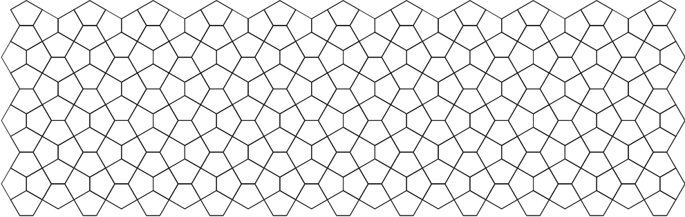
Figure 1: A portion of the Cairo tiling.

The “Cairo tiling” (Figure 1) has many names, as we will see in Section 2. In particular, it is the dual of the snub version of the familiar square tiling. It has two kinds of vertices (i.e. orbits of vertices under its symmetry group) — tetravalent and trivalent.

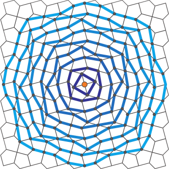
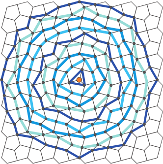
Figure 2: The Cairo tiling has two kinds of vertices (i.e., orbits of vertices under the $4*2$ symmetry group of the tiling) — tetravalent and trivalent. At left, the contour lines of constant distance from a central tetravalent vertex, from which we can read off the first several terms of its CS. At right, contours centered at a trivalent vertex (§6). These contour lines have a recursive and analyzable structure, but we find that the coloring book approach, shown in Figures 5 and 6, is much simpler, allowing more easily verifiable calculations.

It therefore has two coordination sequences (CS’s), giving the numbers $a(n)$ of vertices that are at each distance $n$ from a base vertex $P$, as measured in the graph of edges and vertices in the tiling: those based at either a trivalent or tetravalent vertex. These coordination sequences may be read off from the contour lines, of equal distance from the base vertex $P$ (Figure 2, left and right, respectively). However, although contour lines are structured and can be used to compute CS’s, they are unwieldy to construct and analyze. It is usually easy enough to find the first few terms of the CS, but our goal is to find a formula, recurrence, or generating function for the sequence.

This article was motivated by our recent discovery that the coordination sequence for a tetravalent vertex in the Cairo tiling appeared to be the same as that for the square grid. We thought that such a simple fact should have a simple proof, and this article is the result.

The coloring book approach, described in §3, is an elementary means of calculating coordination sequences, based on coloring the underlying graph with “trunks and branches” and finding a recurrence for the number of vertices at a given distance from the base point. We have to verify that a desired local structure propagates, and that our colored trees do give the correct distance to the base vertex. In §4 we illustrate the method by applying it to an elementary case, the $4^{4}$ square grid tiling.

The method works quite well in many cases and is at least helpful in others: in Sections §5 and §6 we deal with the tetravalent and trivalent vertices in the Cairo tiling and in §7 with its dual, the uniform (or Archimedean) $3^{2}\!.4.3.4$ tiling. We then apply the method to obtain coordination sequences for four other uniform tilings, $3.4.6.4$ (§8), $4.8^{2}$ (§9), $3.12^{2}$ (§10), $3^{4}\!.6$ (§11), and to the dual of the $3^{4}\!.6$ (§12) tiling.

Starting in §10 we must rely on a more subtle analysis, but find that the coloring book method at least renders our calculations somewhat more transparent.

There are of course many works that discuss more sophisticated methods for calculating coordination sequences, in both the crystallographic and mathematical literature, such as Baake & Grimm (1997), Bacher & de la Harpe (2018), Bacher, de la Harpe & Venkov, B. (1997), Conway & Sloane (1997), de la Harpe (2000), Eon (2002, 2004, 2007, 2013, 2016, 2018), Grosse-Kunstleve, Brunner & Sloane (1996), O’Keeffe (1995), and O’Keeffe and Hyde (1980). For a uniform tiling, where the symmetry group acts transitively on the vertices, there is an alternative method for finding CS’s based on Cayley diagrams and the Knuth-Bendix algorithm, and using the computer algebra system Magma (Bosma, Cannon & Playoust, 1997). This approach is briefly described in §13. For uniform tilings it is known (Benson, 1983) that that the CS has a rational generating function. This is also known to be true for other classes of tilings (see the references mentioned at the start of this paragraph). But as far as we know the general conjecture that the CS of a periodic tiling of $n$-dimensional Euclidean space by polytopes always has a rational generating function is still open, even in two dimensions. In this regard, the work of Zhuravlev (2002) and others on the limiting shape of the contour lines in a two-dimensional tiling may be relevant.

A more traditional way to calculate the CS by hand is to draw ‘contour lines’ or ’level curves’ that connect the points at the same distance from $P$. These lines are usually overlaid on top of the tiling. The resulting picture can get very complicated (see Fig. 2), and this approach is usually only successful for simple tilings or for finding just the first few terms of the CS.

“Regular production systems” (Goodman-Strauss, 2009) can be used to give a formal model of growth along a front, enabling generalized contour lines to be described as languages, and underlies some of our thinking here.

The computer program ToposPro (Blatov, Shevchenko & Proserpio, 2014) makes it easy to compute the initial terms of the coordination sequences for a large number of tilings, nets (both two- and three-dimensional), crystal structures, etc.

Besides the obvious application of coordination sequences for estimating the density of points in a tiling, another use is for identifying which tiling or net is being studied. This is especially useful when dealing with three-dimensional structures, as in (Grosse-Kunstleve, Brunner & Sloane,1996). Another application of our coloring-book approach is for finding labels for the vertices in a graph, as we mention at the end of §3.

For any undefined terms about tilings, see the classic work Grünbaum & Shephard (1987) or the article Grünbaum & Shephard (1977).

2 The Cairo tiling

The Cairo tiling is shown in Fig. 1. This beautiful tiling has many names. It has also been called the Cairo pentagonal tiling, the MacMahon net (O’Keeffe & Hyde, 1980), the mcm net (O’Keeffe et al., 2008), the dual of the $3^{2}\dot{4}.3.4$ tiling (Grünbaum & Shephard, 1987, pp. 63, 96, 480 (Fig. $P_{5}$-24)) the dual snub quadrille tiling, or the dual snub square tiling (Conway, Burgiel & Goodman-Strauss, 2008, pp. 263, 288).

 

Figure 1 around here

 

We will refer to it simply as the Cairo tiling. There is only one shape of tile, an irregular pentagon, which may be varied somewhat.

The tiling is named from its use in Cairo, where this pentagonal tile has been mass-produced since at least the 1950’s and is prominent around the city.

 

Figure 2 around here

 

The CS with respect to a tetravalent vertex in the Cairo tiling begins

$$1,4,8,12,16,20,24,28,32,\ldots,$$ (1)

which suggests that it is the same as the CS of the familiar $4^{4}$ square grid (sequence A008574 in the OEIS) . We will show in §5 that this is true, by proving:

Theorem 1.

The coordination sequence with respect to a tetravalent vertex in the Cairo tiling is given by $a(0)=1$, $a(n)=4n$ for $n\geq 1$.

The CS with respect to a trivalent vertex begins

$$1,3,8,12,15,20,25,28,31,36,41,44,47,52,57,60,63,68,73,76,\ldots,$$ (2)

which has now been added to the OEIS as sequence A296368. In §6 we will prove:

Theorem 2.

The coordination sequence with respect to a trivalent vertex in the Cairo tiling is given by $a(0)=1,a(1)=3,a(2)=8$, and, for $n\geq 3$,

$$a(n) \leavevmode\nobreak\ =\leavevmode\nobreak\ 4n\leavevmode\nobreak\ \leavevmode\nobreak\ \leavevmode\nobreak\ \leavevmode\nobreak\ \leavevmode\nobreak\ \mbox{\leavevmode\nobreak\ if\leavevmode\nobreak\ $n$\leavevmode\nobreak\ is\leavevmode\nobreak\ odd}\,,$$

$$\leavevmode\nobreak\ =\leavevmode\nobreak\ 4n-1\mbox{\leavevmode\nobreak\ if\leavevmode\nobreak\ }n\equiv 0\pmod{4}\,,$$

$$\leavevmode\nobreak\ =\leavevmode\nobreak\ 4n+1\mbox{\leavevmode\nobreak\ if\leavevmode\nobreak\ }n\equiv 2\pmod{4}\,.$$ (3)

 

Figure 3 around here

 

The dual of the Cairo tiling is the uniform (or Archimedean) tiling $3^{2}\!.4.3.4$ shown in Fig. 3. Now there is only one kind of vertex, with valency $5$, and the coordination sequence begins

$$1,5,11,16,21,27,32,37,43,48,53,59,64,69,75,80,85,91,96,101,\ldots,$$ (4)

given in A219529. That entry has a long-standing conjecture that $a(n)=\lfloor\frac{16n+1}{3}\rfloor$, and we will establish this in §7 by proving:

Theorem 3.

The coordination sequence with respect to a vertex in the $3^{2}\!.4.3.4$ tiling is given by $a(0)=1$,

$$a(3k) \leavevmode\nobreak\ =\leavevmode\nobreak\ 16k,\leavevmode\nobreak\ k\geq 1\,,$$

$$a(3k+1) \leavevmode\nobreak\ =\leavevmode\nobreak\ 16k+5,\leavevmode\nobreak\ k\geq 0\,,$$

$$a(3k+2) \leavevmode\nobreak\ =\leavevmode\nobreak\ 16k+11,\leavevmode\nobreak\ k\geq 0\,.$$ (5)

3 The coloring book approach to finding coordination sequences

We start with a more precise statement of the problem. Let $T$ be a periodic tiling of the plane by polygonal tiles. The graph $G=G(T)$ of the tiling has a vertex for each point of the plane where three or more tiles meet, and an edge between two vertices if two tiles share a boundary along the line joining the corresponding points.

We assume the tiling is such that $G$ is a connected graph: $G$ is thus a connected, periodic, planar graph with all vertices of valency at least $3$, and (since the tiles are polygons) with no parallel edges. The coloring book method could be applied to any graph of this type, not just one arising from a tiling.

The distance $d(Q,R)$ between vertices $Q$, $R$ in $G$ is defined to be the number of edges in the shortest path joining them. The coordination sequence of $G$ with respect to a vertex $P\in G$ is the sequence $\{a(n):n=0,1,2,\ldots\}$ where $a(n)$ is the number of vertices $Q\in G$ with $d(Q,P)=n$. We refer to $P$ as the base vertex. For a periodic tiling there are only a finite number of different choices for the base vertex, and our goal is to find the coordination sequence with respect to a base vertex of each possible type.

Our method for finding the coordination sequence with respect to a base vertex $P$ is to try to find a subgraph $H$ of $G$ with the following properties.

• $H$ is a connected graph that passes through every vertex of $G$, and

• for any vertex $Q$, every path in $H$ from $Q$ to $P$ has the minimal possible length, $d(Q,P)$.

We also want $H$ to have three further, less well-defined, properties.

• $H$ should be essentially a tree (in the sense of graph theory), and more precisely should consist of a finite number of “trunks” (in the arboreal sense), which are disjoint paths that originate at $P$, together with infinitely many “branches”, which are also disjoint paths and originate at trunk vertices. However, on occasion we will allow the trunks to have “burls” (i.e., bulges, or loops inside the trunk), and both trunks and branches may have “twigs” (typically small subtrees with just a few edges) growing from them.

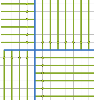
Figure 4: Trunks (blue) and branches (green) for the familiar square tiling, $4^{4}$. Each vertex is associated (via a blue or green edge) with a unique vertex that is one step further away from $P$, except for the vertices on the (blue) trunk, where branches (green) have sprouted. As four branches sprout at each distance $n>0$ from $P$, joining the trunk to the four green vertices, the CS satisfies the recurrence $a(n+1)=a(n)+4$.

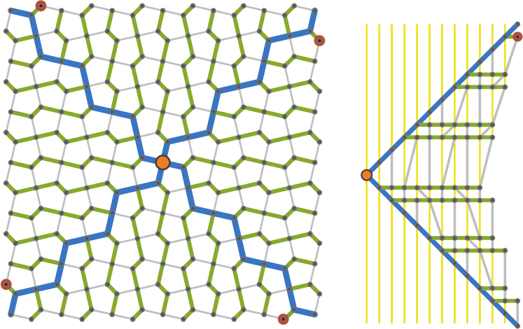
Figure 5: At left, the subgraph $H$ for a tetravalent base vertex in the Cairo tiling. There are four congruent sectors. At right, the right-hand sector of $H$ has been redrawn so that the blue trunks and green branches are straight, with horizontal distances equal to the distance back to $P$ in $G$, in order to show that the (gray) edges not in $H$ do not reduce the distance to the origin. Note that $H$ is transverse to the contour lines, shown in yellow. At each distance $n+1$ from $P$, all but four of the vertices (green) may be associated with the vertices at distance $n$, by tracing back one edge in $H$ — hence $a(n+1)=a(n)+4$. The four red dots on the periphery of the left figure indicate the division into sectors, and help match up the left and right figures.

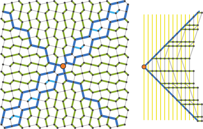
Figure 6: At left, the subgraph $H$ (the blue, green, and light blue edges) for the trivalent case. Two of the trunks have split down the middle, and moreover have sprouted “twigs” (light blue). In the right-hand illustration, the right sector has been redrawn so that the blue trunks and green branches are straight, in order to show that the (gray) edges not in $H$ do not reduce the distances to the origin, and to make it easy to count the vertices at a given distance from the base point.

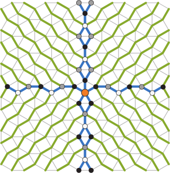
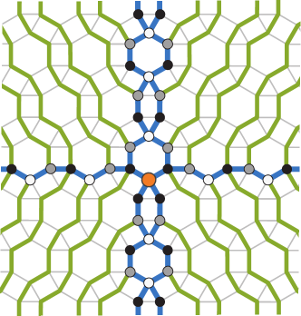
Figure 7: Trunks and branches $H$ for the $3^{2}\!.4.3.4$ tiling, at left and for the $3.4.6.4$ tiling at right. In both drawings, the base vertex $P$ is at the center and vertices on the blue trunks are colored by their distance to $P\mod 3$ — $0$ (white), $1$ (black), or $2$ (gray).

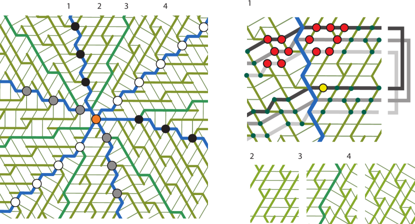
Figure 12: A trunks and branches structure for the $3^{4}\!.6$ tiling (left). The four patterns (1)-(4) that self-perpetuate from level to level (right). In pattern (1), the red vertices at each distance $n+3$ are unmatched at distance $n$, and the yellow vertex at distance $n$ is unmatched at distance $n+3$. For sufficiently large $n$ ($>4$) there are a total of $12$ more vertices at distance $n+3$ than at $n$.

  In our figures, trunks will usually be colored blue) and branches green. A glance at some of the figures below will illustrate our arboreal terminology. In Figs. 4 and 5 (left) $H$ actually is a tree, with simple trunks and branches. In Fig. 6 (left) $H$ is still a tree, but there are twigs (single edges) between the two parallel trunks. In Figs. 7 (left and right) two of the trunks have burls (loops of lengths $4$ and $6$, respectively), and so are not pure trees in the mathematical sense. In Fig. 12 both the trunks and branches have twigs attached.

• There should an easy way to check that Property (ii) holds, i.e., that there are no shortcuts to $P$ that take a path that is not part of $H$.

• And towards this end, $H$ should have some sort of regular structure that allows us to make inductive arguments.

There is no difficulty in satisfying (i), since any spanning tree rooted at P would do. But this is not very helpful since there are an infinite number of distinct spanning trees, and in any case requiring $H$ to be a tree in the mathematical sense can make it harder to satisfy the other conditions.

Assuming that (ii) and (iii) hold, the subgraph $H$ has the following structure. Each trunk out of $P$ is an infinite path, and each trunk vertex (ignoring the slight complication caused by the burls) is joined to a unique trunk vertex that is one step further away from $P$. The branches are infinite paths originating at trunk vertices and (ignoring the twigs) each branch vertex is joined to a unique branch vertex that is one step further away from $P$. The twigs are finite (and small) subtrees that connect any remaining vertices to the closest trunk or branch. If we have carried out (v) well at all, then all these vertices should be easy to count.

As we have gained experience with the method, we have found the following further condition to be helpful for making inductive arguments.

• The distance from any vertex of the tiling to the closest trunk or branch should be bounded. Equivalently, there should be a constant $c_{0}$ such that the twigs have length at most $c_{0}$.

An alternative way to describe $H$ is to think of $G$ as a topographic map, where the heights above sea level of the vertices are the distances from the base point $P$. Then $H$ represents a drainage network that always flows downhill. In this model the ‘trunks’ represent major rivers that flow to $P$, and the ‘branches’ are tributaries that feed into the major rivers.

Speaking informally, the subgraph $H$ is usually orthogonal to the contour lines, just as in polar coordinates, radial lines are orthogonal to the circles.

We have tried a few strategies for finding the subgraph $H$. In several examples (§7-§9), our human visual system seems to fill in the proof of Property (ii) instantly. But a verifiable means of testing (ii) is essential. For the Cairo tiling, we can redraw the graph so that (ii) is clear, as at right in Figures 5 and 6.

As described further in §11, in later examples we use an atlas of patterns, of what locally appear to be trunks and branches, directed across alleged contour lines. These patterns propagate outwards from a region about $P$ — each patch extends outwards in a natural way. Since the alleged contour lines are initially simple nested closed curves, they continue to be so, and therefore are indeed contour lines. Since the alleged trunks and branches are transverse to the contour lines, they are indeed trunks and branches satisfying (ii).

We have found the process of searching for trunks and branches by drawing with colored pencils on pictures of tilings to be quite enjoyable. If readers wish to try this for themselves — and perhaps to improve on our constructions — we encourage them to download pictures of tilings from the Internet. There are many excellent web sites. Galebach’s web site (Galebach 2018) is especially important, as it includes pictures of all $k$-uniform tilings with $k\leq 6$, with over $1000$ tilings. The Chavey (1989) article and the Hartley (2018) and Printable Paper (2018) web sites have many further pictures, and the Reticular Chemistry Structure Resource or RCSR (O’Keeffe et al. 2008) and ToposPro (Blatov et al. 2014) databases have thousands more.

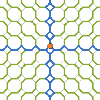
Figure 8: Trunks and branches $H$ for the $4.8^{2}$ tiling, with $P$ at the center and trunks and branches $H$ which clearly propagate and satisfy Property (ii).

In this paper we have been careful to describe our approach as a method for finding coordination sequences, rather than an algorithm. At present we do not have enough experience with the method to state it any more formally. We can point out that periodic two-dimensional tilings by polygons fall into two classes: the essential underlying periodic structure is either rectangular or hexagonal. In the former case one should look for a trunks and branches structure like that shown in Figures 4, 5, 6, 7, 8, and in the latter case like that shown in Figure 12, 15. But as one can see by looking at the catalogs of tilings mentioned above, there is too great a variety of tilings for us to be any more precise than that.

One’s first guess at a trunks and branches structure does not always succeed. For example, in the $3.4.6.4$ tiling, shown at right in Fig. 7, a natural first guess is to make the branches roughly horizontal. However, this does not provide the shortest paths to the origin — for that one needs to use vertical branches that head North-East (in the first quadrant) and North-West (in the second quadrant), as shown in the figure.

There is sometimes another side-benefit to our approach: it may provide a way to assign coordinates to the vertices of the graph. If the branches are paths, and a vertex $Q$ is on a branch that originates at a trunk vertex $R$, then we can label $Q$ by specifying the trunk, the distance $d(R,P)$, the branch, and the distance $d(Q,R)$ (with appropriate modifications in case the trunk or branch is not quite a simple path).

4 The square grid

Before analyzing the Cairo tiling, we illustrate the coloring book method by applying it to a simple case, the $4^{4}$ square tiling seen in graph paper. The subgraph $H$ is shown in Fig. 4.

 

Figure 4 around here

 

For this tiling it is not hard to work out the CS directly, by drawing the contour lines, which are concentric squares centered at the origin. Each new square plainly contains four more vertices than the last one, so the tiling’s CS satisfies the recurrence $a(n+1)=a(n)+4$.

Using the coloring book approach we draw “trunks” (in blue) and “branches” (in green) (see Fig. 4). Each vertex is associated (via a blue or green edge) with a unique vertex that is one step further away from $P$, except for the vertices on the (blue) trunk, where additional branches (green) have sprouted. As four branches sprout at each distance $n$ from $P$ (the vertices marked with a green dot indicate the starts of the branches) the coordination sequence satisfies the recurrence $a(n+1)=a(n)+4$. The recurrence starts with $a(0)=1$, and so we have again shown that $a(n)=1,4,8,12,16,20,\ldots$, as in (1).

5 The Cairo tiling with respect to a tetravalent vertex

At left in Figure 2, the vertices in the Cairo tiling in the vicinity of a tetravalent vertex $P$ are marked by contour lines of constant distance to $P$, and counting the vertices on each contour line confirms that the initial terms of the CS are as shown in (1).

 

Figure 5 around here

 

The subgraph $H$ is shown in Fig. 5 (left). There are four trunks (blue) and infinitely many branches (green), one branch originating at each trunk vertex. Figure 5 (right) shows one sector of $H$ redrawn so that the trunks and branches are straight, and so that we can see they satisfy Property (ii) — that is, using edges that are not part of $H$ (these edges are colored gray) does not provide any shorter paths to the base vertex.

As each vertex on a trunk or branch is associated with another trunk or branch vertex further out, and four new branches are introduced at each distance $n>0$ from the origin, $a(n+1)=a(n)+4$; noting that $a(1)=4$, we have $a(n)=4n$, $n>0$, completing the proof of Theorem 1.

In the redrawn sector on the right of Fig. 5, all the points at a given distance from the base point are colinear, and we see that there are exactly $n-1$ points in the interior of the sector at distance $n$ from the base point. Taking into account the four branch points, we have another proof that $a(n)=4(n-1)+4=4n$ for $n>0$.

Note that there is a unique (green) branch originating at each (blue) trunk vertex. If the trunk vertex is at distance congruent to $1$ or $2\bmod{4}$ from the origin, the branch turns to the left, otherwise it turns to the right.

6 The Cairo tiling with respect to a trivalent vertex

At right in Figure 2 we show the contour lines in the vicinity of a trivalent vertex $P$ in the Cairo tiling, confirming that the initial terms of the CS are as shown in (2).

Because the graph now has only mirror symmetry, the subgraph $H$ is necessarily less elegant than in the tetravalent case. The best choice for $H$ that we have found, shown in Fig. 6, now has six trunks, two of which sprout “twigs” shown in light blue.

 

Figure 6 around here

 

As in Fig. 5, $H$ is naturally divided into four sectors (ignoring the twigs for now). The right and top sectors are congruent to each other, and the left and bottom sectors are essentially the same as any of the sectors in Fig. 5, the main difference being that the base vertices for the left and bottom sectors in Fig. 6 are now one edge away from the origin instead of being at the origin as they were in Fig. 5.

Although there is some variation from level to level, with two out of every three trunk nodes sprouting branches, and taking into account the periodic appearance of twigs, we obtain the recurrence

$$a(n+4)=a(n)+16,\leavevmode\nobreak\ n\geq 3$$

by observing that exactly $16$ branches and twigs sprout in any four consecutive values of $n$, and consequently all but $16$ vertices at distance $n+4$ may be traced back and associated with the vertices at distance $n$, along a trunk, or branch, or from a twig to a closer twig. Verifying the terms $a(0)$ through $a(6)$, we obtain $a(n)$ as in Theorem 2.

Again there is an alternative, more direct, way to see this. In Fig. 6 (right), we see that the vertices at a given distance from the base point are colinear, and for $n\geq 2$ there are $n-2$ interior vertices in the right (and top) sectors if $n\equiv 0$ or $1\pmod{4}$, or $n-1$ if $n\equiv 2$ or $3\pmod{4}$. In each of the left and bottom sectors there are $n-2$ interior vertices (for $n\geq 2$) at distance $n$ from the base point. The numbers of trunk (or dark blue) vertices at distances $0,1,2,3,4,\ldots$ are $1,3,6,6,6,\ldots$, respectively, and the numbers of twig (light blue) vertices at distances $4k$, $4k+1$, $4k+2$, $4k+3$ (for $k\geq 1$) are $1,2,1,0$, respectively. Collecting these values, we obtain equation (2).

7 The $3^{2}\!.4.3.4$ tiling

The $3^{2}\!.4.3.4$ tiling (Fig. 3 in §1) is a uniform tiling: all vertices are equivalent, and we can choose $P$ to be any vertex. As in the previous section, the graph $G$ has only mirror symmetry, and so again we have to accept that our subgraph $H$ of trunks and branches will be less symmetrical that the graph in §5.

In our choice for $H$, shown in Fig. 7, there are two horizontal trunks, but on the vertical trunks some vertices on the vertical branches have been split into “burls” (creating loops of length $4$). With the orientation shown, quadrants I and II are mirror images of each other, as are quadrants III and IV. One can see immediately that any simple path in $H$ from a vertex back to $P$ is as short as any other path back to $P$, and so Property (ii) is satisfied.

 

Figure 7 around here

 

To calculate the coordination sequence, we may note that at any three consecutive distances $n+1$, $n+2$, $n+3$, $n>0$ from $P$, $16$ branches are introduced, and so all but $16$ vertices at distance $n+3$ may be associated with those at distance $n$. This gives us the recurrence $a(n+3)=a(n)+16,n>0$. Checking the terms $a(0)=1,a(1)=5,a(2)=11,a(3)=16$, we obtain (3), and so complete the proof of Theorem 3.

8 The $3.4.6.4$ tiling

Our next example is the $3.4.6.4$ uniform tiling, and we will prove that this too has the same CS as the square grid (this establishes a 2014 conjecture of Darah Chavey stated in A008574).

Theorem 4.

The coordination sequence with respect to a vertex in the $3.4.6.4$ tiling is given by $a(0)=1$, $a(n)=4n$ for $n\geq 1$.

We show our choice of trunks and branches at the right in Fig. 7. As in the left-hand figure, the vertical trunks have split, producing burls which now are chains of hexagons. Again, quadrants I and II are mirror images of each other, as are quadrants III and IV. We can see that Property (ii) is satisfied and that the pattern propagates.

As a total of twelve branches are introduced at three consecutive levels $n+1$, $n+2$, $n+3$, $n>1$, we have the recurrence $a(n+3)=a(n)+12$. Checking the terms up to $a(4)=16$, we complete the proof.

9 The $4.8^{2}$ tiling

 

Figure 8 around here

 

Theorem 5.

The CS (A008576) with respect to a vertex in the $4.8^{2}$ uniform tiling is given by $a(0)=1$ and thereafter $a(3k)=8k$, $a(3k+1)=8k+3$, $a(3k+2)=8k+5$ .

Proof.

The subgraph $H$, shown in at left in Fig. 8 — we again resort to using “burls” but the proof is the same as before: $H$ satisfies Property (ii) and may be propagated; for each $n>1$, at three consecutive distances a total of $24$ branches sprout. Consequently, for $n>1$, $a(n+3)=a(n)+24$. Verifying the terms through $a(4)$, we complete the proof. ∎

 

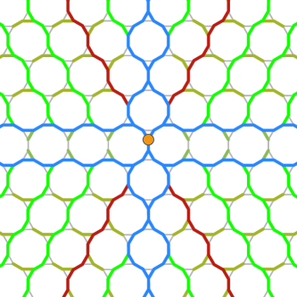
Figure 9: Trunks and branches $H$ for the $3.12^{2}$ tiling, with $P$ at the center and trunks and branches $H$ which clearly propagate and satisfy Property (ii).

Figure 9 around here

 

10 The $3.12^{2}$ tiling

The $3.12^{2}$ uniform tiling is shown in Fig. 9. The CS with respect to any vertex begins

$$1,3,4,6,8,12,14,15,18,21,22,24,28,30,30,33,38,39,38,42,48,\dots\,.$$ (6)

This is sequence A250122, where there is a conjectured formula from 2014 due to Joseph Myers which we can now prove is correct.

Theorem 6.

The coordination sequence for the $3.12^{2}$ tiling is given by $a(0)=1$, $a(1)=3$, $a(2)=4$, and thereafter $a(4k)=10k-2$, $a(4k+1)=9k+3$, $a(4k+2)=8k+6$, and $a(4k+3)=9k+6$.

Proof.

The subgraph $H$ is shown is shown in Fig. 9. There are double trunks along the $x$-axis, and a single trunk with burls along the $y$-axis. The second quadrant is a mirror image of the first, and the third quadrant is a mirror image of the fourth, so we need only analyze the first and fourth quadrants. (The figure is not symmetric about the $x$-axis.) To simplify the discussion we assume the positive $y$-axis points North and the positive $x$-axis points East.

In the first quadrant there are infinitely many parallel branches (green) consisting of infinite paths directed to the North-East, together with twigs (olive green) of length $2$ originating at certain branch vertices. The first quadrant is bisected by one of the branches, let us call it the special branch, indicated by a thick red line, which roughly follows the diagonal $y=x$. To the West of the special branch, the twigs are all directed to the North-West, while to the East of the special branch the twigs are directed to the East.

The situation in the fourth quadrant is similar. There are infinitely many parallel branches (green) consisting of infinite paths directed to the South-East, together with twigs (olive green) of length $2$ originating at certain branch vertices. The fourth quadrant is bisected by one of the branches, the special branch, indicated by a thick red line, which roughly follows the diagonal $y=-x$. To the West of the special branch, the twigs are all directed to the South-West, while to the East of the special branch the twigs are again directed to the East.

 

Table 1 around here

 

Table 1 shows the numbers of vertices of the various types at distance $n$ from the central vertex. The counts depend on the value of $n$ modulo $8$, as indicated by the columns of the table. We assume $n\geq 3$. The rows of the table indicate the different types of vertex. Row (i) refers to the East-West trunks, row (ii) to the North-South trunk, excluding the vertices already counted in (i). Row (iii) counts vertices in the first quadrant that are on and to the East of the special branch, (iv) those to the West of that branch, and (v) counts the twigs. Rows (vi), (vii), (viii) are the analogous counts for the fourth quadrant.The last row of the table gives the grand total, formed by adding the entries in rows (i) and (ii), plus twice (to account for the second and third quadrants) the sum of rows (iii) though (viii).

Examination of the last row shows that the total actually depends only on the value of $n$ modulo $4$, rather than $8$. For example, the assertions that $a(8k)=20k-2$ and $a(8k+4)=20k+8$ can be combined into $a(4k)=10k-2$. Similarly for the other six cases. This completes the proof of the theorem. ∎

11 The $3^{4}\!.6$ tiling

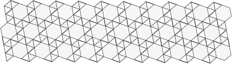
Figure 10: A portion of the $3^{4}\!.6$ uniform tiling.

The $3^{4}\!.6$ uniform tiling is shown in Fig. 10. This is also known as the snub $\{6,3\}$ tiling, and has symmetry group $632$. The CS with respect to any vertex begins

$$1,5,9,15,19,24,29,33,39,43,48,53,57,63,67,72,77,81,87,91,\dots\,.$$ (7)

This is sequence A250120, where there is a conjectured formula from 2014 due to several people, which we can now prove is correct.

 

Figure 10 around here

 

Theorem 7.

The coordination sequence for the $3^{4}\!.6$ tiling is given by $a(0)=1$, $a(1)=5$, $a(2)=9$, $a(3)=15$, $a(4)=19$, $a(5)=24$ and for $n\geq 3$, $a(n+5)=a(n)+24$.

The recurrence can also be written as $a(5k+r)=24k+a(r)$ for $k\geq 0$, $0\leq r\leq 4$.

In all our previous examples, we were able to use the coloring book method to find trunks and branches by simply drawing on a picture of the tiling. This enabled us to calculate the coordination sequence directly, bypassing any complexities in the contour lines. Compare, for example, the contour lines in Fig. 2 with the trunks and branches of Figures 5 and 6, which made the CS for the Cairo tiling a simple calculation. We were happy that this strategy has worked in every case up to this point.

Of course, to use the coloring book method, we must also confirm, in some inductive manner, that the trunks and branches can be continued indefinitely and satisfy Property (ii). For the Cairo tiling, we redrew two of the sectors so as to make it clear that there were patterns of local structure that propagated outwards, maintaining a valid trunks and branches structure that made it easy to compute the CS. We were not as explicit in the next few examples, leaving to the reader the easy verification that the trunks and branches structure propagated. In the present section and the next, however, the structures are more complicated and so we must be more cautious.

We could have always used the contour lines directly, at least in principle — defining the contour lines recursively, with production rules that are constrained by local conditions, as in Goodman-Strauss (2009). For tilings with a co-compact symmetry, such as the ones in this paper, contour lines can be used to conjecture, calculate, and give proofs for the recurrences satisfied by the coordination sequences.

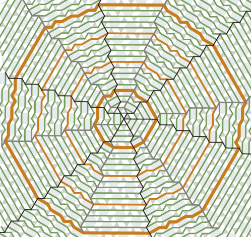
Figure 11: The contour lines of the $3^{4}\!.6$ tiling; their lengths form sequence A250120. The contour lines are partitioned into twelve sectors, alternatively straight and zig-zag. The boundaries zig-zag-to-straight (reading clockwise), drawn in black, have period $3$. The boundaries straight-to-zig-zag, drawn in gray, have period $5$ — in each sector the patterns at the ends of a contour segment have period $15$. A pair of contours $15$ steps apart are emphasized in the figure by heavy brown lines. With patience, after another $15$ steps the regular structure becomes more apparent. Even without doing that, with care one can verify that from each level $n>1$ to level $n+5$, the number of vertices increases by $24$. In Fig. 12, we use a trunks and branches structure to make this more transparent.

The contour lines for the $3^{4}\!.6$ tiling are shown in Fig. 11. From this we can verify that, at least initially, the number of vertices at distance $n>1$ from the base vertex increases by exactly $24$ when $n$ is increased by $5$. Although there appear to be a lot of individual cases to consider, the contours are highly ordered, and the task is primarily one of cataloging the local structures.

 

Figure 11 around here

 

Outside of an initial region about $P$, there are really only four kinds of vertex neighborhoods to consider: vertices where the contour lines are straight, where they zig-zag, and where there is a transition from zig-zag-to-straight and vice versa. In each case, the underlying structure is straightforward and it is easy to see that it propagates from level to level, and also that the structure we see at the center — twelve sectors of alternating types, the six sectors of each type being fundamentally the same — must continue across the entire infinite tiling.

However, there is a further complication: the boundaries between straight-to-zig-zag, drawn in black in Fig. 11, have a period-$3$ pattern, and so the structure of the segments crossing each sector recurs with period $15$.

We now use a trunks and branches approach to simplify this structure, verifying locally that this give the CS, but without needing to check that there is a detailed match with the contour lines.

 

Figure 12 around here

 

The trunks and branches structure is shown on the left in Fig. 12. As in Fig. 7, the base vertex $P$ is at the center and vertices on the blue trunks are colored by their distance to $P\mod 3$ — $0$ (white), $1$ (black), or $2$ (gray). The six trunks each produce a pair of branches and a twig at every third level, but shifted in pairs: all together the trunks sprout four branches and four twigs at each level. On the right in Fig. 12 are shown four patterns (1)-(4) that are self-perpetuating from level to level. If the boundary of a disk can be described by this atlas of patterns, then it is inside a larger disk with the same property — though one must carefully check that every transition from zig-zag-to-straight is of this precise form. By induction, the alleged contour lines in the pattern are nested simple closed curves and so can only lie on actual contour lines; thus the trunks and branches satisfy Property (ii) and correctly give the CS. With the exception of the red and yellow vertices in pattern (1), each vertex at level $n+5$ is naturally matched with a vertex at level $n$, just by following a branch backwards. Notice that the branches have matching twigs at every fifth level. In pattern (1), we examine the mismatched vertices: the red vertices have no match five levels earlier, and the yellow vertex has no match five levels forward. Since pattern (1) repeats at every third level, we have considered all possible cases. At each level, two of the trunks show each of the three cases in pattern (1), so the number of vertices satisfies $a(n+5)=24+a(n)$ for $n\geq 3$, a net increase of six vertices per trunk. After explicitly verifying the initial terms of the coordination sequence, we have completed the proof of Theorem 7.

12 The snub-632 tiling

 

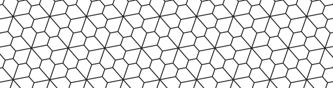
Figure 13: The snub-$632$ tiling.

Figure 13 around here

 

We began this article by analyzing the Cairo tiling, which is the dual to the $3^{2}\!.4.3.4$ uniform tiling. Our final example is the snub-$632$ tiling (Fig. 13), which is the dual to the $3^{4}\!.6$ uniform tiling of the previous section. Like the Cairo tiling, this is a beautiful tiling; fundamentally it is the dual of the snub versions of both the $6^{3}$ and $3^{6}$ tilings. It has several names including:

• the $6$-fold pentille tiling (Conway et al., 2008, p. 288),

• the fsz-d net (O’Keeffe et al. 2008),

• and the dual of the $3^{4}\!.6$ tiling (Grünbaum & Shephard, 1987, pp. 63, 96, 480 (Fig. $P_{5}$-16)).

We will refer to it simply as the snub-$632$ tiling. There is only one shape of tile, an elongated pentagon. There are three types of vertices: (a) hexavalent vertices, with six-fold rotational symmetry, where six long edges of the pentagons meet; (b) trivalent vertices, with three-fold rotational symmetry, where three short edges meet; and (c) trivalent vertices, with no symmetry, where two short edges and one long edge meet. The coordination sequences (A298016, A298015, A298014) for these three types of vertices begin

$$(a)\leavevmode\nobreak\ \leavevmode\nobreak\ 1,6,12,12,24,36,24,42,60,36,60,84,48,78,108,60,96,132,72,\ldots\,,$$

$$(b)\leavevmode\nobreak\ \leavevmode\nobreak\ 1,3,6,15,24,18,33,48,30,51,72,42,69,96,54,87,120,66,105,\ldots\,,$$

$$(c)\leavevmode\nobreak\ \leavevmode\nobreak\ 1,3,9,15,18,27,37,37,44,57,54,61,77,71,78,97,88,95,117,105,\ldots$$ (8)

Theorem 8.

The CS for the three types of vertices in the snub-$632$ tiling are given by:
(a) $a(3k)=12k,\leavevmode\nobreak\ a(3k+1)=18k+6,\leavevmode\nobreak\ a(3k+2)=24k+12$ for $k\geq 1$,
(b) $a(3k)=18k-3,\leavevmode\nobreak\ a(3k+1)=24k,\leavevmode\nobreak\ a(3k+2)=12k+6$ for $k\geq 2$,
(c) $a(3k)=20k-3,\leavevmode\nobreak\ a(3k+1)=17k+3,\leavevmode\nobreak\ a(3k+2)=17k+10$ for $k\geq 2$,
with initial values as in (12). In each case we have $a(n)=2a(n-3)-a(n-6)$ for $n\geq 8$.

 

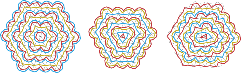
Figure 14: Contour lines in the snub-$632$, centered on a six-fold, three-fold and asymmetric vertex; they are clearly structured and we could compute with them directly. But the coloring book approach simplifies and unifies the count.

Figure 14 around here

 

We could prove Theorem 8 by working directly with the contour lines, shown in Figure 14, and establishing that there is a recursive — although unwieldy — structure for each of the three types of vertices. However, the coloring book approach will enable us to give a uniform treatment.

 

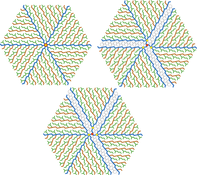
Figure 15: Trunks and branches structures for the three types of base vertices in the the snub-$632$ tiling: (a) (top left), 6-fold base vertex, (b) (top right), 3-fold, (c) (bottom) asymmetric. Each figure is divided into $60$-degree sectors, some of which are separated by channels. The base vertex $P$ is shown in red and the vertices at the apices of the sectors in yellow.

Figure 15 around here

 

Figure 15 shows the trunks and branches structures for the three types of vertices, which we will continue to refer to as cases (a), (b), and (c) for a $6$-fold, $3$-fold, and asymmetric base vertex, respectively. Each figure is divided into $60$-degree sectors, some of which are separated by channels (pairs of parallel branches distance $3$ apart). The individual sectors are all the same, although they differ in how far the apex of the sector (yellow) is from the base vertex (red). In case (a) all six sectors have apex at the base vertex, in case (b) the base vertex is two steps away from the apex, in two different ways, and in case (c) the base vertex is one, two or three steps away from the apex, in six different ways (now each sector has a different displacement from the base vertex).

 

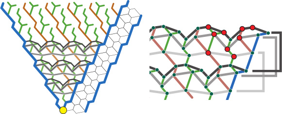
Figure 16: On the left, a sector and a channel, showing trunks (blue), branches (red), twigs (green), and contours (light grey, dark gray, and black) defined by distances to the apex (yellow). In the sector, the vertices at distance $n+3$ from the apex are in one-to-one correspondence with the vertices at distance $n$, with the exception of those shown in red at right. Within each sector, then, for $n$ sufficiently large (that is, beyond the tip of the sector), we obtain a recursion for the number of vertices at distance $n+3$, depending on $n$ modulo $3$. For $n\equiv 0$ there are two more vertices than at distance $n$, for $n\equiv 1$ there are four more, and for $n\equiv 2$ there are three more. In a channel there are the same number of vertices at distance $n+3$ as for $n$. In the text we complete the calculation across the whole tiling.

Figure 16 around here

 

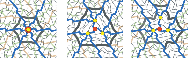
Figure 17: The contour lines near $P$ in each of the cases (a), (b) and (c).

Figure 16 shows a sector (internally they are all the same) with a channel next to it. The sector is bounded by two trunks (blue) and has a pattern of branches (red) and twigs (green). The figure also shows the contour lines defined by the distances to the apex (yellow). Contours at distances congruent to $0$, $1$, and $2$ mod $3$ from the apex are colored light gray, dark gray, and black, respectively. A crucial step in the analysis is that these contour lines are still the contour lines with respect to the base vertex, even when the base vertex is at one of the other eight possible vertices — there are no shortcuts to the base vertex. Of course the distances from the contours to the base vertex get increased by one, two, or three steps when the base vertex is moved. We return to this point in Fig. 17.

In the sector, the vertices at distance $n+3$ from the apex are in one-to-one correspondence with the vertices at distance $n$, with the exception (and this is the other crucial step) of the nine vertices shown in red on the right of Fig. 16. There are two unmatched vertices at distance $0\bmod{3}$ from the apex (on the light gray curve), three at distance $1\bmod{3}$ (on the dark gray curve) and four at distance $2\bmod{3}$ (on the black curve). As the structure along a trunk repeats with period $3$, this includes all the possibilities. The vertices that are not in any sector are in exact correspondence with those three steps further away.

The detailed book-keeping for case (c) is as follows; (a) and (b) are simpler and are discussed below.

In case (c), take $n$ sufficiently large, which turns out to mean $n>5$, that being the distance from $P$ to where the regular structure starts to be self-perpetuating. There is one sector with apex at distance $3$; so from P, there are, for

$n\equiv 0\mod 3$,	two unmatched vertices at distance $n+3$,
$n\equiv 1\mod 3$,	three unmatched at $n+3$,
$n\equiv 2\mod 3$,	four unmatched at $n+3$.

There are two sectors with apex at distance $2$, so from P there are, for

$n\equiv 2\mod 3$, twice two unmatched vertices at distance $n+3$,

$n\equiv 0\mod 3$, twice three unmatched at $n+3$,

$n\equiv 1\mod 3$, twice four unmatched at $n+3$.

There are three sectors with apex at distance $1$, so from P there are, for

$n\equiv 1\mod 3$, three times two unmatched vertices at distance $n+3$,

$n\equiv 2\mod 3$, three times three unmatched at $n+3$,

$n\equiv 0\mod 3$, three times four unmatched at $n+3$

In summary, for case (c) there are three sectors with apex at distance $1$ from $P$, two at distance $2$ and one at distance $3$. The vertices in the channels do not contribute to the recursion (since the vertices at distance $n+3$ are in one-to-one correspondence with those at distance $n$, for $n>2$). For case (c) we therefore have the recurrence, for $k>1$,

$a(3k+6)=3\cdot 4+2\cdot 3+1\cdot 2+a(3k+3)$,

$a(3k+7)=3\cdot 2+2\cdot 4+1\cdot 3+a(3k+4)$,

$a(3k+8)=3\cdot 3+2\cdot 2+1\cdot 4+a(3k+5)$.

In case (a), there are six sectors, each with apex at distance $0$ from $P$. The recurrence is therefore, for $k>1$, $a(3k+3)=6\cdot 2+a(3k)$, $a(3k+4)=6\cdot 3+a(3k+1)$, $a(3k+5)=6\cdot 4+a(3k+2)$.

For case (b), there are six sectors, each with apex at distance $2$ from $P$, and the recurrence is, for $k>1$, $a(3k+5)=6\cdot 2+a(3k+2)$, $a(3k+6)=6\cdot 3+a(3k+3)$, $a(3k+7)=6\cdot 4+a(3k+4)$.

After verifying the initial terms by hand, we recover the sequences stated in the theorem.

However, as mentioned above, we must still check that even when the base vertex $P$ is not at the apex, the contour lines measured from $P$ really do cross the sectors and their trunks and branches structures as shown in Figure 16. This check is carried out in Figure 17. The heavy lines indicate where the regular structure — the recurrence — begins.

 

Figure 17 around here

 

13 Cayley diagrams and growth series

If the symmetry group of the tiling acts transitively on the vertices, and the subgroup fixing a vertex is the trivial group, it is possible to represent the graph of the tiling as a Cayley diagram for an appropriate presentation of the group. For example, consider the $4.8^{2}$ tiling shown in Fig. 8. Every vertex is trivalent, with one edge (denoted by ‘$o$’, say) separating two adjacent octagons, and a pair of edges (‘$\ell$’ and ‘$r$’) that go either to the left or the right around the adjacent square. Let $R$ mean ‘move along the edge $o$’, and let $S$ mean ‘move along the edge $\ell$’. Applying $R$ twice returns one to the start, which we indicate by saying that $R^{2}=1$. Similarly, $S^{4}=1$ (going around the square) and $(RS)^{4}=1$ (going around an octagon). The group $G$ generated by $R$ and $S$ subject to these relations, specified by the presentation

$$G\leavevmode\nobreak\ =\leavevmode\nobreak\ \langle R,S\mid R^{2}=S^{4}=(RS)^{4}=1\rangle\,,$$ (9)

assigns a unique label to each vertex in the graph. In technical terms, this gives an identification of the graph of the tiling with the Cayley diagram of the group defined by this presentation (Johnson 1976).

The ‘length’ of a group element is the minimal number of generators needed to represent it, which is also its distance from the identity element in the Cayley diagram. The ‘growth function’ for the group specifies the number of elements of each length $n$, and so the growth function is precisely the coordination sequence for the tiling. For the graphs of uniform tilings, the Knuth-Bendix algorithm (Knuth & Bendix, 1989), Epstein et al., 1991) can be used to solve the word problem and determine the growth function. This algorithm is implemented in the GrowthFunction command in the computer algebra system Magma (Bosma et al. 1997). When applied to the presentation (9), for example, Magma returns the generating function

$$\sum_{n=0}^{\infty}a(n)x^{n}\leavevmode\nobreak\ =\leavevmode\nobreak\ \frac{(1+x)^{2}}{(1-x)^{2}}\,,$$

which is equivalent to the formulas given in Theorem 5.

 

Table 2 around here

 

Table 2 lists presentations for all eleven uniform two-dimensional tilings. We have verified that the resulting growth functions coincide with the coordination sequences given in earlier sections and in the OEIS.

Presentations for the $17$ planar crystallographic groups can be found in Table 3 of Coxeter & Moser (1984), and Shutov (2003) used them to compute coordination sequences for the corresponding directed Cayley graphs. Eon (2018) gives presentations for the eleven uniform tilings and points out the connection between the Cayley diagrams and the graphs of the tilings. However, neither article uses these presentations to explicitly compute the coordination sequences for the tilings.

It is worth pointing out that the growth series approach to finding coordination sequences used in this section only applies when the graph of the tiling coincides with the Cayley graph of some group, whereas our coloring book approach can potentially be applied to any periodic tiling.

Acknowledgments We thank Davide M. Proserpio for telling us about the RCSR and ToposPro websites, and for drawing our attention to the articles Eon (2018) and Shutov (2013). Davide M. Proserpio has also helped by using ToposPro to compute coordination sequences for many tilings, not mentioned in this article, which are now included in the OEIS.

After seeing a preliminary version of this article, Jean-Guillaume Eon commented that the coloring book method might be viewed as complementary to the algebraic method introduced in Eon (2002). The labeled quotient graph of the net or tiling from that article could help to find the subgraph $H$ needed for our approach, and conversely, using $H$ instead of the quotient graph may simplify finding the the coordination sequence.

It will be interesting to see if a combination of our methods will lead to proofs of the conjectured formulas for some of the more complicated tilings, such as those of the $20$ $2$-uniform tilings. A list of these $2$-uniform tilings and their coordination sequences (and conjectured formulas) may be found in entry A301724 in the OEIS. Perhaps once these and other tilings have been analyzed, it will be possible to state a more precise algorithmic version of the coloring book method.

We also thank the referees for their helpful comments.

             

Figure 3: A portion of the $3^{2}\!.4.3.4$ uniform tiling, the dual to the Cairo structure. Distances to $P$ (which is the red vertex in the center of the figure) are shown in various colors, illustrating terms $a(0)$, …, $a(6)$ of the coordination sequence, A219529. In Figure 7, the count is clarified by a trunks and branches structure.

             

Table 1: Calculation of coordination sequence for $3.12.12$ tiling. Top row gives distance $n$ from central vertex, rows indicate the eight types of vertex, last row is grand total.

$$\begin{array}[]{c|cccccccc}n:&8k&8k+1&8k+2&8k+3&8k+4&8k+5&8k+6&8k+7\\ \hline\cr(i)&4&6&6&4&4&6&6&4\\ (ii)&2&3&4&4&4&4&4&3\\ (iii)&k&k&k&k&k&k&k+1&k+1\\ (iv)&2k-1&2k-1&2k-1&2k-1&2k&2k&2k&2k\\ (v)&2k-1&2k-1&k&k&2k&2k&k&k\\ (vi)&k&k&k&k&k&k+1&k+1&k+1\\ (vii)&2k-1&2k-1&2k-1&2k&2k&2k&2k&2k+1\\ (viii)&2k-1&k&k&2k&2k&k&k&2k+1\\ \hline\cr a(n)&20k-2&18k+3&16k+6&18k+6&20k+8&18k+12&16k+14&18k+15\end{array}$$

Table 2: Presentations for the groups of the eleven uniform tilings, giving section number if mentioned above, number of generators $g$, and corresponding sequence number.

$$\begin{array}[]{lllll}\mbox{Tiling}&$\S$&g&\mbox{Presentation}&\mbox{Sequence}\\ 3^{6}&&3&RST=1,RS=SR&{\underline{A008458}}\\ 3^{4}\!.6&\ref{Sec33336}&3&R^{2}=S^{3}=T^{6}=RST=1&{\underline{A250120}}\\ 3^{3}\!.4^{2}&&4&R^{2}=T^{2}=U^{2}=SUT=1,RS=SR&{\underline{A008706}}\\ 3^{2}\!.4.3.4&\ref{SecDual}&3&R^{2}=RST=(ST^{-1})^{2}=1&{\underline{A219529}}\\ 3.4.6.4&\ref{Sec3464}&2&R^{3}=S^{6}=RSRS=1&{\underline{A008574}}\\ 3.6.3.6&&2&R^{3}=S^{3}=(RS)^{3}=1&{\underline{A008579}}\\ 3.12^{2}&\ref{Sec31212}&2&R^{2}=S^{3}=(RS)^{6}=1&{\underline{A250122}}\\ 4^{4}&\ref{SecM}&2&RS=SR&{\underline{A008574}}\\ 4.6.12&&3&R^{2}=S^{2}=T^{2}=(TS)^{2}=(RT)^{3}=(SR)^{6}=1&{\underline{A072154}}\\ 4.8^{2}&\ref{Sec488}&2&R^{2}=S^{4}=(RS)^{4}=1&{\underline{A008576}}\\ 6^{3}&&3&R^{2}=S^{2}=T^{2}=1,RST=TSR&{\underline{A008486}}\\ \end{array}$$