IFIC/18-004

CFTP/18-004

Flavour Conservation in Two Higgs Doublet Models

Francisco J. Botella ^a,, Fernando Cornet-Gomez ^a,, Miguel Nebot ^b,

^a Departament de Física Teòrica and IFIC,
Universitat de València-CSIC,
E-46100, Burjassot, Spain.

^b Centro de Física Teórica de Partículas (CFTP),
Instituto Superior Técnico (IST), U. de Lisboa (UL),
Av. Rovisco Pais, P-1049-001 Lisboa, Portugal.

In extensions of the Standard Model with two Higgs doublets, flavour changing Yukawa couplings of the neutral scalars may be present at tree level. In this work we consider the most general scenario in which those flavour changing couplings are absent. We revise the conditions that the Yukawa coupling matrices must obey for such general flavour conservation (gFC), and study the one loop renormalisation group evolution of such conditions in both the quark and lepton sectors. We show that gFC in the leptonic sector is one loop stable under the Renormalization Group Evolution (RGE) and in the quark sector we present some new Cabibbo like solution also one loop stable under RGE. At a phenomenological level, we obtain the regions for the different gFC parameters that are allowed by the existing experimental constraints related to the 125 GeV Higgs.

1 Introduction

Two Higgs Doublet Models (2HDM) [1, 2, 3] are a simple and popular class of extensions of the Standard Model (SM). Besides the original motivation, in particular the possibility of having spontaneous CP violation [1], extending the SM scalar sector with a second doublet allows a number of interesting phenomenological consequences. To name a few generic ones: the appearance of new fundamental scalar particles, non-standard properties of the “quite Higgs-like” scalar discovered at the LHC with a mass of 125 GeV [4, 5], and, related to them, a number of potential deviations in low energy processes with respect to SM expectations. They have been the focus of intense scrutiny before and after the 2012 discovery [6, 7, 8, 9, 10, 11, 12, 13, 14, 15, 16, 17, 18, 19, 20, 21, 22, 23, 24, 25, 26, 27, 28]. Additional aspects, including dark matter candidates [29, 30] or sources of CP violation in addition to the Cabibbo-Kobayashi-Maskawa matrix [31, 32, 33], of interest for baryogenesis [34, 35, 36], provide further interest in 2HDM.

In the SM, concentrating on quarks, a single Yukawa structure in each sector – up and down – is both responsible for: (i) the generation of mass upon spontaneous breaking of $SU(2)_{\rm L}\otimes U(1)_{\rm Y}$ into $U(1)_{\rm EM}$, and (ii) the couplings of the quarks to the only fundamental scalar leftover, the Higgs boson, after associating the three would-be Goldstone bosons to the longitudinal polarizations of the massive $Z$ and $W^{\pm}$ gauge bosons. As a consequence, there are no tree level Flavour Changing Neutral Couplings (FCNC) of the Higgs to quarks. With two independent Yukawa structures available in each sector, the situation is dramatically changed in the general 2HDM, and FCNC couplings of quarks do arise at tree level. To which extent they appear in the couplings of the different physical neutral scalars depends then on the details of the scalar potential [37]: if the 125 GeV scalar is a mixture of the true-but-unphysical Higgs and the additional neutral scalars, FCNC “leak” into its couplings through that mixing. At the end of the day, as with many New Physics avenues, the presence of FCNC is a double edged feature: since the competing SM gauge mediated contributions to FCNC processes are loop induced, those transitions pose severe constraints while, on the same grounds, provide immediate opportunities to discover deviations from the SM picture.

The study of different ways to dispense without problematic too large FCNC couplings and the conditions for their appearance or absence, has drawn sustained attention over the years. As analysed in [38, 39], the absence of FCNC is guaranteed by forcing each right-handed fermion type to couple to one and only one scalar doublet; this absence of FCNC, backed by a $\mathbb{Z}_{2}$ symmetry, is a popular option, and several implementations of this Natural Flavour Conservation (NFC) idea, namely 2HDM of types I, II, and of types X, Y (when the lepton sector is also considered) have been thoroughly explored. Additional $U(1)$ gauge symmetries have also been considered, for example, in [40, 41]. The general conditions for the absence of FCNC, that is, that the mass matrix and the remaining Yukawa coupling matrix can be diagonalised simultaneously, were identified early [42, 43, 44, 45]. The interplay of how a symmetry requirement could enforce that general NFC and shed some light into the structure of the resulting CKM matrix was addressed in [46, 42, 47, 48, 49, 50, 51, 52, 53] with interesting consequences.

On a different line of thought, stepping back from right out forbiddance, suppression of FCNC in other “natural” manners has also attracted significant interest, including suppression given by masses like in the Cheng-Sher ansätz [54], suppression obtained from broken/approximate flavour symmetries [55, 56, 57, 58], and symmetry controlled FCNC scenarios [59, 60, 61, 62, 63]. Among the later, Branco-Grimus-Lavoura (BGL) models are worth mentioning in particular, since this suppression is simply given by products of CKM matrix elements [64, 65] (see also related extensions [66, 67, 68]). In a more recent popular scenario, the Aligned 2HDM [69], the absence of FCNC is a priori achieved (and parametrised) with simple requirements on the Yukawa couplings (for an early mention of this kind of possibility, although in the context of real Yukawa couplings and spontaneous CP violation, see also [70]). The possibility of having effective aligned scenarios has been studied in [71, 72]. Radiative effects and the interplay of tree level FCNC with the Renormalization Group Evolution (RGE) have also been addressed by and large in the literature [73, 49, 9, 74, 75, 76, 77, 78, 79].

The aim of this work is to explore different facets of scenarios with general flavour conservation (gFC), i.e. generalised flavour alignment, in 2HDM; in other words, analysing relevant aspects of the most general 2HDM scenarios where tree level FCNC are, a priori, absent. An analysis of FCNC induced in this context by the RGE has been recently presented in [80]. On a purely phenomenological basis, a scenario of this type restricted to the lepton sector was also considered in [81, 82].

The paper is organised as follows. In section 2, we revisit some generalities of 2HDM, fix the notation for the discussion to follow, and recall the most relevant aspects of the conditions leading to gFC. They are then analysed attending to the Renormalization Group Evolution that they obey in section 3, leading to the full set of conditions required to have RGE-stable gFC. The well known type I and type II cases are briefly revisited in section 3.3; section 3.5 is devoted to a particular solution which arises when the CKM matrix is reduced to a single Cabibbo-like mixing. The gFC stability of the lepton sector is discussed in section 3.4. In section 4, we discuss the most relevant experimental constraints on gFC arising from flavour conserving Higgs-related observables, leading to the analysis and results of section 4.4.
Appendix A provides details omitted in the discussion of section 3.

2 Yukawa Couplings and General Flavour Conservation

The Higgs doublets ($j=1,2$) of 2HDM are

$$\Phi_{j}=e^{i\theta_{j}}\begin{pmatrix}\varphi_{j}^{+}\\ (v_{j}+\rho_{j}+i\eta_{j})/\sqrt{2}\end{pmatrix}$$ (1)

where $v_{j}$, $\theta_{j}$ are real numbers, $\rho_{j}$, $\eta_{j}$, are neutral (hermitian) fields and $\varphi_{j}^{\pm}$ are charged fields. Equation (1) anticipates the assumption that the scalar potential $V(\Phi_{1},\Phi_{2})$ [2, 3] is such that $V(\langle\Phi_{1}\rangle,\langle\Phi_{2}\rangle)$ has an appropriate minimum at

$$\langle\Phi_{j}\rangle=\begin{pmatrix}0\\ e^{i\theta_{j}}v_{j}/\sqrt{2}\end{pmatrix}\,.$$ (2)

In the “Higgs basis” [37, 7, 83], only one linear combination of $\Phi_{1}$ and $\Phi_{2}$, $H_{1}$, has a non-vanishing vacuum expectation value,

$$\begin{pmatrix}H_{1}\\ H_{2}\end{pmatrix}=\mathcal{R}_{\beta}\begin{pmatrix}e^{-i\theta_{1}}\Phi_{1}\\ e^{-i\theta_{2}}\Phi_{2}\end{pmatrix},\quad\langle H_{1}\rangle=\frac{v}{\sqrt{2}}\begin{pmatrix}0\\ 1\end{pmatrix},\quad\langle H_{2}\rangle=\begin{pmatrix}0\\ 0\end{pmatrix},$$ (3)

with $v=\sqrt{v_{1}^{2}+v_{2}^{2}}$, $c_{\beta}=\cos\beta\equiv v_{1}/v$, $s_{\beta}=\sin\beta=v_{2}/v$ and

$$\mathcal{R}_{\beta}\equiv\begin{pmatrix}c_{\beta}&s_{\beta}\\ -s_{\beta}&\phantom{-}c_{\beta}\end{pmatrix}\,,\ [\mathcal{R}_{\beta}]^{-1}=[\mathcal{R}_{\beta}]^{T}\,.$$ (4)

The expansion of $H_{1}$, $H_{2}$ around that minimum of the potential reads

$$H_{1}=\begin{pmatrix}G^{+}\\ (v+\mathrm{H}^{0}+iG^{0})/\sqrt{2}\end{pmatrix},\quad H_{2}=\begin{pmatrix}\mathrm{H}^{+}\\ (\mathrm{R}^{0}+i\mathrm{I}^{0})/\sqrt{2}\end{pmatrix},$$ (5)

where

$$\begin{pmatrix}G^{+}\\ \mathrm{H}^{+}\end{pmatrix}=\mathcal{R}_{\beta}\begin{pmatrix}\varphi_{1}^{+}\\ \varphi_{2}^{+}\end{pmatrix},\ \begin{pmatrix}G^{0}\\ \mathrm{I}^{0}\end{pmatrix}=\mathcal{R}_{\beta}\begin{pmatrix}\eta_{1}\\ \eta_{2}\end{pmatrix},\ \begin{pmatrix}\mathrm{H}^{0}\\ \mathrm{R}^{0}\end{pmatrix}=\mathcal{R}_{\beta}\begin{pmatrix}\rho_{1}\\ \rho_{2}\end{pmatrix}.$$ (6)

The would-be Goldstone bosons $G^{0}$ and $G^{\pm}$ provide the longitudinal degrees of freedom of the $Z$ and $W^{\pm}$ gauge bosons; furthermore, while $\mathrm{H}^{\pm}$ is already a physical charged scalar field, the physical neutral scalars $\{\mathrm{h},\mathrm{H},\mathrm{A}\}$ are real linear combinations of $\{\mathrm{H}^{0},\mathrm{R}^{0},\mathrm{I}^{0}\}$,

$$\mathcal{R}_{\mathrm{[3]}}(\vec{\alpha})\,\begin{pmatrix}\mathrm{h}\\ \mathrm{H}\\ \mathrm{A}\end{pmatrix}=\begin{pmatrix}\mathrm{H}^{0}\\ \mathrm{R}^{0}\\ \mathrm{I}^{0}\end{pmatrix}\,,\ [\mathcal{R}_{\mathrm{[3]}}(\vec{\alpha})]^{-1}=[\mathcal{R}_{\mathrm{[3]}}(\vec{\alpha})]^{T}\,,$$ (7)

with $[\mathcal{R}_{\mathrm{[3]}}(\vec{\alpha})]$ a real orthogonal rotation described by three real mixing angles, $\vec{\alpha}=\{\alpha_{12},\alpha_{13},\alpha_{23}\}$ ($c_{x}\equiv\cos x$, $s_{x}\equiv\sin x$),

$$[\mathcal{R}_{\mathrm{[3]}}(\vec{\alpha})]=\begin{pmatrix}c_{\alpha_{12}}&-s_{\alpha_{12}}&0\\ s_{\alpha_{12}}&c_{\alpha_{12}}&0\\ 0&0&1\end{pmatrix}\,\begin{pmatrix}c_{\alpha_{13}}&0&-s_{\alpha_{13}}\\ 0&1&0\\ s_{\alpha_{13}}&0&c_{\alpha_{13}}\end{pmatrix}\,\begin{pmatrix}1&0&0\\ 0&c_{\alpha_{23}}&-s_{\alpha_{23}}\\ 0&s_{\alpha_{23}}&c_{\alpha_{23}}\end{pmatrix}\,.$$ (8)

When there is no CP violation in the scalar potential, i.e. no mixing connecting the CP-even $\mathrm{H}^{0}$, $\mathrm{R}^{0}$, and the CP-odd $\mathrm{I}^{0}$, it is customary to introduce the mixing angle $\alpha$

$$\begin{pmatrix}\mathrm{h}\\ \mathrm{H}\end{pmatrix}=\begin{pmatrix}\phantom{-}s_{\alpha}&c_{\alpha}\\ -c_{\alpha}&s_{\alpha}\end{pmatrix}\begin{pmatrix}\rho_{1}\\ \rho_{2}\end{pmatrix}=\begin{pmatrix}\phantom{-}s_{\beta\alpha}&c_{\beta\alpha}\\ -c_{\beta\alpha}&s_{\beta\alpha}\end{pmatrix}\begin{pmatrix}\mathrm{H}^{0}\\ \mathrm{R}^{0}\end{pmatrix}$$ (9)

where $s_{\beta\alpha}=\sin(\alpha+\beta)$ and $c_{\beta\alpha}=\cos(\alpha+\beta)$ (that is, $\alpha_{13}=\alpha_{23}=0$ and $\alpha_{12}=\pi/2-(\alpha+\beta)$ in Eq. (8)). Since a $\pm$ sign can be included in the definition of the scalar fields without changing their kinetic terms, different conventions for Eqs. (8)–(9) are used in the literature, which may be relevant when comparing expressions.

2.1 Quark Yukawa Couplings in 2HDM

The Yukawa couplings of the quarks – $SU(2)_{L}$ doublets $Q_{L}^{0}$ and singlets $d_{R}^{0}$, $u_{R}^{0}$ – with the scalar doublets read

$$\mathscr{L}_{\rm Y}^{[q]}=-\bar{Q}_{L}^{0}[\Gamma^{\phantom{\dagger}}_{1}\Phi_{1}+\Gamma^{\phantom{\dagger}}_{2}\Phi_{2}]d_{R}^{0}-\bar{Q}_{L}^{0}[\Delta^{\phantom{\dagger}}_{1}\tilde{\Phi}_{1}+\Delta^{\phantom{\dagger}}_{2}\tilde{\Phi}_{2}]u_{R}^{0}+\text{H.c.}$$ (10)

with $\tilde{\Phi}_{j}=i\sigma_{2}\Phi_{j}^{\ast}$. Following Eqs. (3)–(5),

$$\mathscr{L}_{\rm Y}^{[q]}= -\frac{\sqrt{2}}{v}\bar{Q}_{L}^{0}[\mathcal{M}^{0}_{\mathrm{d}}H_{1}+\mathcal{N}^{0}_{\mathrm{d}}H_{2}]d_{R}^{0}-\frac{\sqrt{2}}{v}\bar{Q}_{L}^{0}[\mathcal{M}^{0}_{\mathrm{u}}\tilde{H}_{1}+\mathcal{N}^{0}_{\mathrm{u}}\tilde{H}_{2}]u_{R}^{0}+\text{H.c.}$$ (11)

$$= \,\mathscr{L}_{\rm m}^{[q]}+\mathscr{L}_{\rm G}^{[q]}+\mathscr{L}_{\rm Ch}^{[q]}+\mathscr{L}_{\rm N}^{[q]}$$ (12)

with mass terms $\mathscr{L}_{\rm m}^{[q]}$, would-be Goldstone boson couplings $\mathscr{L}_{\rm G}^{[q]}$, and Yukawa couplings to charged and neutral scalars, $\mathscr{L}_{\rm Ch}^{[q]}$ and $\mathscr{L}_{\rm N}^{[q]}$:

$$\mathscr{L}_{\rm m}^{[q]}\supset -\bar{d}_{L}^{0}\mathcal{M}^{0}_{\mathrm{d}}d_{R}^{0}-\bar{u}_{L}^{0}\mathcal{M}^{0}_{\mathrm{u}}u_{R}^{0}\,,$$ (13)

$$\mathscr{L}_{\rm G}^{[q]}\supset -\frac{\sqrt{2}}{v}\left[G^{+}\bar{u}_{L}^{0}\mathcal{M}^{0}_{\mathrm{d}}d_{R}^{0}+iG^{0}\bar{d}_{L}^{0}\mathcal{M}^{0}_{\mathrm{d}}d_{R}^{0}-G^{-}\bar{d}_{L}^{0}\mathcal{M}^{0}_{\mathrm{u}}u_{R}^{0}-iG^{0}\bar{u}_{L}^{0}\mathcal{M}^{0}_{\mathrm{u}}u_{R}^{0}\right],$$ (14)

$$\mathscr{L}_{\rm Ch}^{[q]}\supset -\frac{\sqrt{2}}{v}\left[\mathrm{H}^{+}\bar{u}_{L}^{0}\mathcal{N}^{0}_{\mathrm{d}}d_{R}^{0}-\mathrm{H}^{-}\bar{d}_{L}^{0}\mathcal{N}^{0}_{\mathrm{u}}u_{R}^{0}\right],$$ (15)

$$\mathscr{L}_{\rm N}^{[q]}\supset -\frac{1}{v}\left[\mathrm{H}^{0}\bar{d}_{L}^{0}\mathcal{M}^{0}_{\mathrm{d}}d_{R}^{0}+(\mathrm{R}^{0}+i\mathrm{I}^{0})\bar{d}_{L}^{0}\mathcal{N}^{0}_{\mathrm{d}}d_{R}^{0}+\mathrm{H}^{0}\bar{u}_{L}^{0}\mathcal{M}^{0}_{\mathrm{u}}u_{R}^{0}+(\mathrm{R}^{0}-i\mathrm{I}^{0})\bar{u}_{L}^{0}\mathcal{N}^{0}_{\mathrm{u}}u_{R}^{0}\right].$$ (16)

The mass matrices are

$$\mathcal{M}^{0}_{\mathrm{d}}=\frac{v}{\sqrt{2}}\left[e^{i\theta_{1}}c_{\beta}\Gamma^{\phantom{\dagger}}_{1}+e^{i\theta_{2}}s_{\beta}\Gamma^{\phantom{\dagger}}_{2}\right],\quad\mathcal{M}^{0}_{\mathrm{u}}=\frac{v}{\sqrt{2}}\left[e^{-i\theta_{1}}c_{\beta}\Delta^{\phantom{\dagger}}_{1}+e^{-i\theta_{2}}s_{\beta}\Delta^{\phantom{\dagger}}_{2}\right],$$ (17)

and the second linear combinations of Yukawa matrices which encode the potential FCNC are

$$\mathcal{N}^{0}_{\mathrm{d}}=\frac{v}{\sqrt{2}}\left[-e^{i\theta_{1}}s_{\beta}\Gamma^{\phantom{\dagger}}_{1}+e^{i\theta_{2}}c_{\beta}\Gamma^{\phantom{\dagger}}_{2}\right],\quad\mathcal{N}^{0}_{\mathrm{u}}=\frac{v}{\sqrt{2}}\left[-e^{-i\theta_{1}}s_{\beta}\Delta^{\phantom{\dagger}}_{1}+e^{-i\theta_{2}}c_{\beta}\Delta^{\phantom{\dagger}}_{2}\right]\,.$$ (18)

For the usual bi-diagonalisation of the mass matrices $\mathcal{M}^{0}_{\mathrm{d}}$, $\mathcal{M}^{0}_{\mathrm{u}}$, the quark mass eigenstates (without “0” superscript) read

$$d_{L}=U_{{\rm d_{L}}}^{\dagger}d_{L}^{0},\ d_{R}=U_{{\rm d_{R}}}^{\dagger}d_{R}^{0},\ u_{L}=U_{{\rm u_{L}}}^{\dagger}u_{L}^{0},\ u_{R}=U_{{\rm u_{R}}}^{\dagger}u_{R}^{0},$$ (19)

with

$$\mathcal{M}_{\mathrm{d}}=U_{{\rm d_{L}}}^{\dagger}\mathcal{M}^{0}_{\mathrm{d}}\,U_{{\rm d_{R}}}^{\phantom{\dagger}}=\text{diag}(m_{d},m_{s},m_{b})\,,\ \mathcal{M}_{\mathrm{u}}=U_{{\rm u_{L}}}^{\dagger}\mathcal{M}^{0}_{\mathrm{u}}\,U_{{\rm u_{R}}}^{\phantom{\dagger}}=\text{diag}(m_{u},m_{c},m_{t})\,,$$ (20)

$$\mathcal{N}_{\mathrm{d}}=U_{{\rm d_{L}}}^{\dagger}\mathcal{N}^{0}_{\mathrm{d}}\,U_{{\rm d_{R}}}^{\phantom{\dagger}}\,,\ \mathcal{N}_{\mathrm{u}}=U_{{\rm u_{L}}}^{\dagger}\mathcal{N}^{0}_{\mathrm{u}}\,U_{{\rm u_{R}}}^{\phantom{\dagger}}\,.$$ (21)

The CKM matrix is $V=U_{{\rm u_{L}}}^{\dagger}U_{{\rm d_{L}}}^{\phantom{\dagger}}$. When both $\mathcal{N}_{\mathrm{d}}$ and $\mathcal{N}_{\mathrm{u}}$ are diagonal, tree-level FCNC are absent.
Expressing Eq. (11) in terms of quark and scalar mass eigenstates (as a shorthand we use $[\mathcal{R}_{\mathrm{[3]}}(\vec{\alpha})]_{ij}=\mathcal{R}_{ij}$),

$$\mathscr{L}_{\rm m}^{[q]}= -\bar{d}_{L}\mathcal{M}_{\mathrm{d}}d_{R}-\bar{u}_{L}\mathcal{M}_{\mathrm{u}}u_{R}+\text{H.c.}\,,$$ (22)

$$\mathscr{L}_{\rm G}^{[q]}= -\frac{\sqrt{2}}{v}\left[G^{+}\bar{u}_{L}V\mathcal{M}_{\mathrm{d}}d_{R}+iG^{0}\bar{d}_{L}\mathcal{M}_{\mathrm{d}}d_{R}+G^{-}\bar{d}_{L}V^{\dagger}\mathcal{M}_{\mathrm{u}}u_{R}-iG^{0}\bar{u}_{L}\mathcal{M}_{\mathrm{u}}u_{R}\right]+\text{H.c.},$$ (23)

$$\mathscr{L}_{\rm Ch}^{[q]}=-\frac{\sqrt{2}}{v}\left\{\mathrm{H}^{+}\left[\bar{u}_{L}V\mathcal{N}_{\mathrm{d}}d_{R}-\bar{u}_{R}\mathcal{N}^{\dagger}_{\mathrm{u}}Vd_{L}\right]+\mathrm{H}^{-}\left[\bar{d}_{R}\mathcal{N}^{\dagger}_{\mathrm{d}}V^{\dagger}u_{L}-\bar{d}_{L}V^{\dagger}\mathcal{N}_{\mathrm{u}}u_{R}\right]\right\},$$ (24)

$$\mathscr{L}_{\rm N}^{[q]}= -\frac{\mathrm{h}}{v}\left\{\bar{d}\left[\mathcal{R}_{11}\mathcal{M}_{\mathrm{d}}+\mathcal{R}_{21}\mathcal{H}_{\mathrm{d}}+i\mathcal{R}_{31}\mathcal{A}_{\mathrm{d}}\right]d+\bar{d}\left[\mathcal{R}_{21}\mathcal{A}_{\mathrm{d}}+i\mathcal{R}_{31}\mathcal{H}_{\mathrm{d}}\right]\gamma_{5}d\right\}$$

$$-\frac{\mathrm{h}}{v}\left\{\bar{u}\left[\mathcal{R}_{11}\mathcal{M}_{\mathrm{u}}+\mathcal{R}_{21}\mathcal{H}_{\mathrm{u}}-i\mathcal{R}_{31}\mathcal{A}_{\mathrm{u}}\right]u+\bar{u}\left[\mathcal{R}_{21}\mathcal{A}_{\mathrm{u}}-i\mathcal{R}_{31}\mathcal{H}_{\mathrm{u}}\right]\gamma_{5}u\right\}$$

$$-\frac{\mathrm{H}}{v}\left\{\bar{d}\left[\mathcal{R}_{12}\mathcal{M}_{\mathrm{d}}+\mathcal{R}_{22}\mathcal{H}_{\mathrm{d}}+i\mathcal{R}_{32}\mathcal{A}_{\mathrm{d}}\right]d+\bar{d}\left[\mathcal{R}_{22}\mathcal{A}_{\mathrm{d}}+i\mathcal{R}_{32}\mathcal{H}_{\mathrm{d}}\right]\gamma_{5}d\right\}$$

$$-\frac{\mathrm{H}}{v}\left\{\bar{u}\left[\mathcal{R}_{12}\mathcal{M}_{\mathrm{u}}+\mathcal{R}_{22}\mathcal{H}_{\mathrm{u}}-i\mathcal{R}_{32}\mathcal{A}_{\mathrm{u}}\right]u+\bar{u}\left[\mathcal{R}_{22}\mathcal{A}_{\mathrm{u}}-i\mathcal{R}_{32}\mathcal{H}_{\mathrm{u}}\right]\gamma_{5}u\right\}$$

$$-\frac{\mathrm{A}}{v}\left\{\bar{d}\left[\mathcal{R}_{13}\mathcal{M}_{\mathrm{d}}+\mathcal{R}_{23}\mathcal{H}_{\mathrm{d}}+i\mathcal{R}_{33}\mathcal{A}_{\mathrm{d}}\right]d+\bar{d}\left[\mathcal{R}_{23}\mathcal{A}_{\mathrm{d}}+i\mathcal{R}_{33}\mathcal{H}_{\mathrm{d}}\right]\gamma_{5}d\right\}$$

$$-\frac{\mathrm{A}}{v}\left\{\bar{u}\left[\mathcal{R}_{13}\mathcal{M}_{\mathrm{u}}+\mathcal{R}_{23}\mathcal{H}_{\mathrm{u}}-i\mathcal{R}_{33}\mathcal{A}_{\mathrm{u}}\right]u+\bar{u}\left[\mathcal{R}_{23}\mathcal{A}_{\mathrm{u}}-i\mathcal{R}_{33}\mathcal{H}_{\mathrm{u}}\right]\gamma_{5}u\right\},$$ (25)

where

$$\mathcal{H}_{\mathrm{q}}\equiv\frac{\mathcal{N}_{\mathrm{q}}+\mathcal{N}^{\dagger}_{\mathrm{q}}}{2},\quad\mathcal{A}_{\mathrm{q}}\equiv\frac{\mathcal{N}_{\mathrm{q}}-\mathcal{N}^{\dagger}_{\mathrm{q}}}{2},\quad q=u,d,$$ (26)

are the hermitian and anti-hermitian combinations of $\mathcal{N}_{\mathrm{q}}$ and $\mathcal{N}^{\dagger}_{\mathrm{q}}$.
With no CP violation in the scalar sector,

$$\mathcal{R}=\begin{pmatrix}s_{\beta\alpha}&-c_{\beta\alpha}&0\\ c_{\beta\alpha}&\phantom{-}s_{\beta\alpha}&0\\ 0&0&1\end{pmatrix}\,,$$ (27)

and Eq. (25) reduces to

$$\mathscr{L}_{\rm N}^{[q]}= -\frac{\mathrm{h}}{v}\left\{\bar{d}\left[s_{\beta\alpha}\mathcal{M}_{\mathrm{d}}+c_{\beta\alpha}\mathcal{H}_{\mathrm{d}}\right]d+c_{\beta\alpha}\,\bar{d}\mathcal{A}_{\mathrm{d}}\gamma_{5}d\right\}$$

$$-\frac{\mathrm{h}}{v}\left\{\bar{u}\left[s_{\beta\alpha}\mathcal{M}_{\mathrm{u}}+c_{\beta\alpha}\mathcal{H}_{\mathrm{u}}\right]u+c_{\beta\alpha}\,\bar{u}\mathcal{A}_{\mathrm{u}}\gamma_{5}u\right\}$$

$$-\frac{\mathrm{H}}{v}\left\{\bar{d}\left[-c_{\beta\alpha}\mathcal{M}_{\mathrm{d}}+s_{\beta\alpha}\mathcal{H}_{\mathrm{d}}\right]d+s_{\beta\alpha}\,\bar{d}\mathcal{A}_{\mathrm{d}}\gamma_{5}d\right\}$$

$$-\frac{\mathrm{H}}{v}\left\{\bar{u}\left[-c_{\beta\alpha}\mathcal{M}_{\mathrm{u}}+s_{\beta\alpha}\mathcal{H}_{\mathrm{u}}\right]u+s_{\beta\alpha}\,\bar{u}\mathcal{A}_{\mathrm{u}}\gamma_{5}u\right\}$$

$$-i\frac{\mathrm{A}}{v}\left\{\bar{d}\mathcal{A}_{\mathrm{d}}d+\bar{d}\mathcal{H}_{\mathrm{d}}\gamma_{5}d\right\}+i\frac{\mathrm{A}}{v}\left\{\bar{u}\mathcal{A}_{\mathrm{u}}u+\bar{u}\mathcal{H}_{\mathrm{u}}\gamma_{5}u\right\}.$$ (28)

2.2 Lepton Yukawa Couplings in 2HDM

The Yukawa couplings of the lepton $SU(2)_{L}$ doublets $L_{L}^{0}$ and singlets $\ell_{R}^{0}$ with the scalar doublets are

$$\mathscr{L}_{\rm Y}^{[\ell]}=-\bar{L}_{L}^{0}(\Pi^{\phantom{\dagger}}_{1}\Phi_{1}+\Pi^{\phantom{\dagger}}_{2}\Phi_{2})\ell_{R}^{0}+\text{H.c.}=-\frac{\sqrt{2}}{v}\bar{L}_{L}^{0}(\mathcal{M}^{0}_{\mathrm{\ell}}H_{1}+\mathcal{N}^{0}_{\mathrm{\ell}}H_{2})\ell_{R}^{0}+\text{H.c.}$$ (29)

where, similarly to the quark sector in the previous section,

$$\mathcal{M}^{0}_{\mathrm{\ell}}=\frac{v}{\sqrt{2}}\left[e^{i\theta_{1}}c_{\beta}\Pi^{\phantom{\dagger}}_{1}+e^{i\theta_{2}}s_{\beta}\Pi^{\phantom{\dagger}}_{2}\right],\quad\mathcal{N}^{0}_{\mathrm{\ell}}=\frac{v}{\sqrt{2}}\left[-e^{i\theta_{1}}s_{\beta}\Pi^{\phantom{\dagger}}_{1}+e^{i\theta_{2}}c_{\beta}\Pi^{\phantom{\dagger}}_{2}\right].$$ (30)

The mass eigenstates, without “0” superscript, correspond to

$$\ell_{L}=U_{{\rm\ell_{L}}}^{\dagger}\ell_{L}^{0},\quad\ell_{R}=U_{{\rm\ell_{R}}}^{\dagger}\ell_{R}^{0},$$ (31)

and

$$\mathcal{M}_{\mathrm{\ell}}=U_{{\rm\ell_{L}}}^{\dagger}\,\mathcal{M}^{0}_{\mathrm{\ell}}\,U_{{\rm\ell_{R}}}^{\phantom{\dagger}}=\text{diag}(m_{e},m_{\mu},m_{\tau}),\quad\mathcal{N}_{\mathrm{\ell}}=U_{{\rm\ell_{L}}}^{\dagger}\,\mathcal{N}^{0}_{\mathrm{\ell}}\,U_{{\rm\ell_{R}}}^{\phantom{\dagger}}\,.$$ (32)

Notice that we do not include right-handed neutrinos $\nu_{R}^{0}$ and thus, unlike in the quark sector, there is only one set of Yukawa coupling matrices and we work in the massless neutrino approximation. The leptonic analogs of the Yukawa couplings in Eqs. (24)-(25) are

$$\mathscr{L}_{\rm Ch}^{[\ell]}=-\frac{\sqrt{2}}{v}\left\{\mathrm{H}^{+}\bar{\nu}_{L}\mathcal{N}_{\mathrm{\ell}}\ell_{R}+\mathrm{H}^{-}\bar{\ell}_{R}\mathcal{N}^{\dagger}_{\mathrm{\ell}}\nu_{L}\right\},$$ (33)

$$\mathscr{L}_{\rm N}^{[\ell]}= -\frac{\mathrm{h}}{v}\left\{\bar{\ell}\left[\mathcal{R}_{11}\mathcal{M}_{\mathrm{\ell}}+\mathcal{R}_{21}\mathcal{H}_{\mathrm{\ell}}+i\mathcal{R}_{31}\mathcal{A}_{\mathrm{\ell}}\right]\ell+\bar{\ell}\left[\mathcal{R}_{21}\mathcal{A}_{\mathrm{\ell}}+i\mathcal{R}_{31}\mathcal{H}_{\mathrm{\ell}}\right]\gamma_{5}\ell\right\}$$

$$-\frac{\mathrm{H}}{v}\left\{\bar{\ell}\left[\mathcal{R}_{12}\mathcal{M}_{\mathrm{\ell}}+\mathcal{R}_{22}\mathcal{H}_{\mathrm{\ell}}+i\mathcal{R}_{32}\mathcal{A}_{\mathrm{\ell}}\right]\ell+\bar{\ell}\left[\mathcal{R}_{22}\mathcal{A}_{\mathrm{\ell}}+i\mathcal{R}_{32}\mathcal{H}_{\mathrm{\ell}}\right]\gamma_{5}\ell\right\}$$

$$-\frac{\mathrm{A}}{v}\left\{\bar{\ell}\left[\mathcal{R}_{13}\mathcal{M}_{\mathrm{\ell}}+\mathcal{R}_{23}\mathcal{H}_{\mathrm{\ell}}+i\mathcal{R}_{33}\mathcal{A}_{\mathrm{\ell}}\right]\ell+\bar{\ell}\left[\mathcal{R}_{23}\mathcal{A}_{\mathrm{\ell}}+i\mathcal{R}_{33}\mathcal{H}_{\mathrm{\ell}}\right]\gamma_{5}\ell\right\},$$ (34)

with

$$\mathcal{H}_{\mathrm{\ell}}\equiv\frac{\mathcal{N}_{\mathrm{\ell}}+\mathcal{N}^{\dagger}_{\mathrm{\ell}}}{2},\quad\mathcal{A}_{\mathrm{\ell}}\equiv\frac{\mathcal{N}_{\mathrm{\ell}}-\mathcal{N}^{\dagger}_{\mathrm{\ell}}}{2}.$$ (35)

2.3 General Flavour Conservation

The necessary and sufficient conditions obeyed by the quark Yukawa coupling matrices $\Gamma^{\phantom{\dagger}}_{\alpha}$, $\Delta^{\phantom{\dagger}}_{\alpha}$, $\alpha=1,2$, in order to have gFC [42, 43, 44, 45], are that each of the sets

$$\{\Gamma^{\phantom{\dagger}}_{\alpha}\Gamma^{\dagger}_{\beta}\},\ \{\Gamma^{\dagger}_{\alpha}\Gamma^{\phantom{\dagger}}_{\beta}\},\ \{\Delta^{\phantom{\dagger}}_{\alpha}\Delta^{\dagger}_{\beta}\},\ \{\Delta^{\dagger}_{\alpha}\Delta^{\phantom{\dagger}}_{\beta}\},\quad\alpha,\beta=1,2,$$ (36)

is abelian, that is, their elements commute:

$$\left[\Gamma^{\phantom{\dagger}}_{\alpha}\Gamma^{\dagger}_{\beta}\,,\,\Gamma^{\phantom{\dagger}}_{\gamma}\Gamma^{\dagger}_{\delta}\right]=0,\ \left[\Gamma^{\dagger}_{\alpha}\Gamma^{\phantom{\dagger}}_{\beta}\,,\,\Gamma^{\dagger}_{\gamma}\Gamma^{\phantom{\dagger}}_{\delta}\right]=0,\ \left[\Delta^{\phantom{\dagger}}_{\alpha}\Delta^{\dagger}_{\beta}\,,\,\Delta^{\phantom{\dagger}}_{\gamma}\Delta^{\dagger}_{\delta}\right]=0,\ \left[\Delta^{\dagger}_{\alpha}\Delta^{\phantom{\dagger}}_{\beta}\,,\,\Delta^{\dagger}_{\gamma}\Delta^{\phantom{\dagger}}_{\delta}\right]=0,$$ (37)

with $\alpha,\beta,\gamma,\delta=1,2$. In that case, $\{\Gamma^{\phantom{\dagger}}_{1},\Gamma^{\phantom{\dagger}}_{2}\}$ are simultaneously bi-diagonalised, and $\{\Delta^{\phantom{\dagger}}_{1},\Delta^{\phantom{\dagger}}_{2}\}$ too.
A crucial corollary to these necessary and sufficient conditions is the fact that the simultaneous diagonalisability is intrinsic to the Yukawa coupling matrices themselves, independently of the spontaneous symmetry breaking vacuum characterised by the VEVs $v_{1},v_{2}$. In other words, the property is independent of $\beta$ in Eqs. (17), (18); the simultaneous bi-diagonalisability of $\{\mathcal{M}^{0}_{\mathrm{q}},\mathcal{N}^{0}_{\mathrm{q}}\}$ is equivalent to the simultaneous bi-diagonalisability of the Yukawa couplings matrices or of any other independent linear combinations of them. Of course, the actual values of the eigenvalues of both $\mathcal{M}^{0}_{\mathrm{q}}$ (the masses) and $\mathcal{N}^{0}_{\mathrm{q}}$ do depend on the particular linear combinations.
For leptons, similarly, $\{\Pi^{\phantom{\dagger}}_{\alpha}\Pi^{\dagger}_{\beta}\}$ and $\{\Pi^{\dagger}_{\alpha}\Pi^{\phantom{\dagger}}_{\beta}\}$ must be abelian in order to have gFC, and the previous corollary applies equally to them.
A very relevant consequence follows [46, 42, 47, 48, 49, 50, 51, 52, 53]: if gFC is due to the Lagrangian in Eq. (10) being invariant under a (symmetry) transformation of quarks and scalars, the CKM mixing matrix cannot be related to the values of the masses; for example, predictions being made at the time (late 70’s) for the Cabibbo angle, like $\tan\theta_{c}=m_{d}/m_{s}$ [84, 85], could not lead simultaneously to gFC. Moreover, the resulting mixings are unrealistic (for example, no mixing or a permutation times a complex phase) and radiative corrections cannot be invoked to yield realistic mixings [49].
The most general parameterisation of tree level couplings of fermions to scalars obeying gFC is, quite trivially,

$$\mathcal{N}_{\mathrm{d}}=\begin{pmatrix}n_{d}&0&0\\ 0&n_{s}&0\\ 0&0&n_{b}\end{pmatrix}\!,\ \mathcal{N}_{\mathrm{u}}=\begin{pmatrix}n_{u}&0&0\\ 0&n_{c}&0\\ 0&0&n_{t}\end{pmatrix}\!,\ \mathcal{N}_{\mathrm{\ell}}=\begin{pmatrix}n_{e}&0&0\\ 0&n_{\mu}&0\\ 0&0&n_{\tau}\end{pmatrix}\!,\quad n_{j}\in\mathbb{C},$$ (38)

which we use in the rest of the paper: in section 3 for the study of the renormalization group evolution and in section 4 for a phenomenological analysis.
Notice that, while for the flavour changing couplings the simultaneous presence of scalar and pseudoscalar terms in fermion-scalar Yukawa interactions is not necessarily CP violating, in the diagonal, flavour conserving ones, on the contrary, it is CP violating (see for example [86]). With the flavour conserving matrices $\mathcal{N}_{\mathrm{f}}$ in Eq. (38), the hermitian and antihermitian couplings in Eqs. (28) and (34) are, respectively, their real and imaginary parts. For example, for a CP conserving scalar sector with non-zero mixing $c_{\beta\alpha}\neq 0$, if $\mathcal{N}_{\mathrm{f}}$ are not real, they constitute new sources of CP violation in neutral couplings. For the couplings to the charged scalar, without entering into details, if $\text{Im}(n_{u_{i}}n_{d_{j}})\neq 0$, the combination of scalar and pseudoscalar terms in the coupling $\mathrm{H}^{+}\bar{u}_{i}\,d_{j}$ is CP violating.

3 Renormalization Group Evolution and Flavour Conservation

3.1 Evolution of the Quark Yukawa Coupling Matrices

The one loop evolution of the Yukawa couplings under the renormalization group [75, 76, 87, 77] is (with $\mathcal{D}\equiv 16\pi^{2}\frac{d}{d\ln\mu}$ and $\mu$ the energy scale):

$$\mathcal{D}\Gamma^{\phantom{\dagger}}_{\alpha}=a_{d}\Gamma^{\phantom{\dagger}}_{\alpha}+\sum_{\rho=1}^{n=2}T^{d}_{\alpha,\rho}\Gamma^{\phantom{\dagger}}_{\rho}+\sum_{\rho=1}^{n=2}\left(-2\Delta^{\phantom{\dagger}}_{\rho}\Delta^{\dagger}_{\alpha}\Gamma^{\phantom{\dagger}}_{\rho}+\Gamma^{\phantom{\dagger}}_{\alpha}\Gamma^{\dagger}_{\rho}\Gamma^{\phantom{\dagger}}_{\rho}+\frac{1}{2}\Delta^{\phantom{\dagger}}_{\rho}\Delta^{\dagger}_{\rho}\Gamma^{\phantom{\dagger}}_{\alpha}+\frac{1}{2}\Gamma^{\phantom{\dagger}}_{\rho}\Gamma^{\dagger}_{\rho}\Gamma^{\phantom{\dagger}}_{\alpha}\right)\\ \text{with }T^{d}_{\alpha,\rho}\equiv 3\,\text{tr}\left(\Gamma^{\phantom{\dagger}}_{\alpha}\Gamma^{\dagger}_{\rho}+\Delta^{\dagger}_{\alpha}\Delta^{\phantom{\dagger}}_{\rho}\right)+\text{tr}\left(\Pi^{\phantom{\dagger}}_{\alpha}\Pi^{\dagger}_{\rho}\right),$$ (39)

$$\mathcal{D}\Delta^{\phantom{\dagger}}_{\alpha}=a_{u}\Delta^{\phantom{\dagger}}_{\alpha}+\sum_{\rho=1}^{n=2}T^{u}_{\alpha,\rho}\Delta^{\phantom{\dagger}}_{\rho}+\sum_{\rho=1}^{n=2}\left(-2\Gamma^{\phantom{\dagger}}_{\rho}\Gamma^{\dagger}_{\alpha}\Delta^{\phantom{\dagger}}_{\rho}+\Delta^{\phantom{\dagger}}_{\alpha}\Delta^{\dagger}_{\rho}\Delta^{\phantom{\dagger}}_{\rho}+\frac{1}{2}\Gamma^{\phantom{\dagger}}_{\rho}\Gamma^{\dagger}_{\rho}\Delta^{\phantom{\dagger}}_{\alpha}+\frac{1}{2}\Delta^{\phantom{\dagger}}_{\rho}\Delta^{\dagger}_{\rho}\Delta^{\phantom{\dagger}}_{\alpha}\right)\\ \text{with }T^{u}_{\alpha,\rho}\equiv 3\,\text{tr}\left(\Delta^{\phantom{\dagger}}_{\alpha}\Delta^{\dagger}_{\rho}+\Gamma^{\dagger}_{\alpha}\Gamma^{\phantom{\dagger}}_{\rho}\right)+\text{tr}\left(\Pi^{\dagger}_{\alpha}\Pi^{\phantom{\dagger}}_{\rho}\right)=T^{d\,\ast}_{\alpha,\rho}\,,$$ (40)

where

$$a_{d}=-8g_{s}^{2}-\frac{9}{4}g^{2}-\frac{5}{12}g^{\prime 2},\qquad a_{u}=a_{d}-g^{\prime 2},$$ (41)

with $g_{s}$, $g$, $g^{\prime}$ the gauge coupling constants of $SU(3)_{c}$, $SU(2)_{L}$ and $U(1)_{Y}$, respectively. Introducing

$${\Large\Gamma}_{L}=\sum_{\rho=1}^{n=2}\Gamma^{\phantom{\dagger}}_{\rho}\Gamma^{\dagger}_{\rho}\,,\quad{\Large\Gamma}_{R}=\sum_{\rho=1}^{n=2}\Gamma^{\dagger}_{\rho}\Gamma^{\phantom{\dagger}}_{\rho}\,,\quad{\large\Delta}_{L}=\sum_{\rho=1}^{n=2}\Delta^{\phantom{\dagger}}_{\rho}\Delta^{\dagger}_{\rho}\,,\quad\text{and}\quad{\large\Delta}_{R}=\sum_{\rho=1}^{n=2}\Delta^{\dagger}_{\rho}\Delta^{\phantom{\dagger}}_{\rho}\,,$$ (42)

Eqs. (39)–(40) read

$$\mathcal{D}\Gamma^{\phantom{\dagger}}_{\alpha}=a_{d}\Gamma^{\phantom{\dagger}}_{\alpha}+\sum_{\rho=1}^{n=2}T^{d}_{\alpha,\rho}\Gamma^{\phantom{\dagger}}_{\rho}+\Gamma^{\phantom{\dagger}}_{\alpha}{\Large\Gamma}_{R}+\frac{1}{2}{\Large\Gamma}_{L}\Gamma^{\phantom{\dagger}}_{\alpha}+\frac{1}{2}{\large\Delta}_{L}\Gamma^{\phantom{\dagger}}_{\alpha}-2\sum_{\rho=1}^{n=2}\Delta^{\phantom{\dagger}}_{\rho}\Delta^{\dagger}_{\alpha}\Gamma^{\phantom{\dagger}}_{\rho}\,,$$ (43)

$$\mathcal{D}\Delta^{\phantom{\dagger}}_{\alpha}=a_{u}\Delta^{\phantom{\dagger}}_{\alpha}+\sum_{\rho=1}^{n=2}T^{u}_{\alpha,\rho}\Delta^{\phantom{\dagger}}_{\rho}+\Delta^{\phantom{\dagger}}_{\alpha}{\large\Delta}_{R}+\frac{1}{2}{\large\Delta}_{L}\Delta^{\phantom{\dagger}}_{\alpha}+\frac{1}{2}{\Large\Gamma}_{L}\Delta^{\phantom{\dagger}}_{\alpha}-2\sum_{\rho=1}^{n=2}\Gamma^{\phantom{\dagger}}_{\rho}\Gamma^{\dagger}_{\alpha}\Delta^{\phantom{\dagger}}_{\rho}\,.$$ (44)

Equations (43)–(44) are the starting point to analyse the one loop stability of the necessary and sufficient conditions for gFC. For that, one needs to know

$$\mathcal{D}\left(\left[\Gamma^{\phantom{\dagger}}_{\alpha}\Gamma^{\dagger}_{\beta}\,,\,\Gamma^{\phantom{\dagger}}_{\gamma}\Gamma^{\dagger}_{\delta}\right]\right),\,\mathcal{D}\left(\left[\Gamma^{\dagger}_{\alpha}\Gamma^{\phantom{\dagger}}_{\beta}\,,\,\Gamma^{\dagger}_{\gamma}\Gamma^{\phantom{\dagger}}_{\delta}\right]\right),\,\mathcal{D}\left(\left[\Delta^{\phantom{\dagger}}_{\alpha}\Delta^{\dagger}_{\beta}\,,\,\Delta^{\phantom{\dagger}}_{\gamma}\Delta^{\dagger}_{\delta}\right]\right),\,\mathcal{D}\left(\left[\Delta^{\dagger}_{\alpha}\Delta^{\phantom{\dagger}}_{\beta}\,,\,\Delta^{\dagger}_{\gamma}\Delta^{\phantom{\dagger}}_{\delta}\right]\right),$$ (45)

under the assumption that Eq. (37) holds. With that objective in mind, some simplifications are worth mentioning. Starting with $\Gamma^{\phantom{\dagger}}_{\alpha}\Gamma^{\dagger}_{\beta}$, we first notice that

$$\mathcal{D}(\Gamma^{\phantom{\dagger}}_{\alpha}\Gamma^{\dagger}_{\beta})=(\mathcal{D}\Gamma^{\phantom{\dagger}}_{\alpha})\Gamma^{\dagger}_{\beta}+\Gamma^{\phantom{\dagger}}_{\alpha}(\mathcal{D}\Gamma^{\phantom{\dagger}}_{\beta})^{\dagger}=f^{\rm[d_{L}]}_{\alpha\beta}(\Gamma)+g^{\rm[d_{L}]}_{\alpha\beta}(\Gamma,\Delta)\,,$$ (46)

with

$$f^{\rm[d_{L}]}_{\alpha\beta}(\Gamma)=2a_{d}\Gamma^{\phantom{\dagger}}_{\alpha}\Gamma^{\dagger}_{\beta}+\sum_{\rho=1}^{n=2}\left[T^{d}_{\alpha,\rho}\Gamma^{\phantom{\dagger}}_{\rho}\Gamma^{\dagger}_{\beta}+T^{d\ast}_{\beta,\rho}\Gamma^{\phantom{\dagger}}_{\alpha}\Gamma^{\dagger}_{\rho}\right]+2\Gamma^{\phantom{\dagger}}_{\alpha}{\Large\Gamma}_{R}\Gamma^{\dagger}_{\beta}+\frac{1}{2}{\Large\Gamma}_{L}\Gamma^{\phantom{\dagger}}_{\alpha}\Gamma^{\dagger}_{\beta}+\frac{1}{2}\Gamma^{\phantom{\dagger}}_{\alpha}\Gamma^{\dagger}_{\beta}{\Large\Gamma}_{L}\,,$$ (47)

and

$$g^{\rm[d_{L}]}_{\alpha\beta}(\Gamma,\Delta)=\frac{1}{2}{\large\Delta}_{L}\Gamma^{\phantom{\dagger}}_{\alpha}\Gamma^{\dagger}_{\beta}+\frac{1}{2}\Gamma^{\phantom{\dagger}}_{\alpha}\Gamma^{\dagger}_{\beta}{\large\Delta}_{L}-2\sum_{\rho=1}^{n=2}\left[\Delta^{\phantom{\dagger}}_{\rho}\Delta^{\dagger}_{\alpha}\Gamma^{\phantom{\dagger}}_{\rho}\Gamma^{\dagger}_{\beta}+\Gamma^{\phantom{\dagger}}_{\alpha}\Gamma^{\dagger}_{\rho}\Delta^{\phantom{\dagger}}_{\beta}\Delta^{\dagger}_{\rho}\right].$$ (48)

The relevant property of the decomposition in Eq. (46) is that $f^{\rm[d_{L}]}_{\alpha\beta}$ depends only, in terms of matrices, on $\Gamma\Gamma^{\dagger}$ and $\Gamma\Gamma^{\dagger}\Gamma\Gamma^{\dagger}$ terms, while $g^{\rm[d_{L}]}_{\alpha\beta}$ collects the remaining dependence on $\Delta$’s, which has terms $\Gamma\Gamma^{\dagger}\Delta\Delta^{\dagger}$ and $\Delta\Delta^{\dagger}\Gamma\Gamma^{\dagger}$. Then,

$$\mathcal{D}\left[\Gamma^{\phantom{\dagger}}_{\alpha}\Gamma^{\dagger}_{\beta}\,,\,\Gamma^{\phantom{\dagger}}_{\gamma}\Gamma^{\dagger}_{\delta}\right]=\left[\mathcal{D}(\Gamma^{\phantom{\dagger}}_{\alpha}\Gamma^{\dagger}_{\beta})\,,\,\Gamma^{\phantom{\dagger}}_{\gamma}\Gamma^{\dagger}_{\delta}\right]+\left[\Gamma^{\phantom{\dagger}}_{\alpha}\Gamma^{\dagger}_{\beta}\,,\,\mathcal{D}(\Gamma^{\phantom{\dagger}}_{\gamma}\Gamma^{\dagger}_{\delta})\right]=\\ \left[f^{\rm[d_{L}]}_{\alpha\beta}(\Gamma)+g^{\rm[d_{L}]}_{\alpha\beta}(\Gamma,\Delta)\,,\,\Gamma^{\phantom{\dagger}}_{\gamma}\Gamma^{\dagger}_{\delta}\right]+\left[\Gamma^{\phantom{\dagger}}_{\alpha}\Gamma^{\dagger}_{\beta}\,,\,f^{\rm[d_{L}]}_{\gamma\delta}(\Gamma)+g^{\rm[d_{L}]}_{\gamma\delta}(\Gamma,\Delta)\right]\,.$$ (49)

3.2 Evolution with gFC Matrices

It is clear that, if there is gFC, i.e. with Eq. (37),

$$\left[f^{\rm[d_{L}]}_{\alpha\beta}(\Gamma)\,,\,\Gamma^{\phantom{\dagger}}_{\gamma}\Gamma^{\dagger}_{\delta}\right]=\left[\Gamma^{\phantom{\dagger}}_{\alpha}\Gamma^{\dagger}_{\beta}\,,\,f^{\rm[d_{L}]}_{\gamma\delta}(\Gamma)\right]=0\,,$$ (50)

and thus

$$\mathcal{D}\left[\Gamma^{\phantom{\dagger}}_{\alpha}\Gamma^{\dagger}_{\beta}\,,\,\Gamma^{\phantom{\dagger}}_{\gamma}\Gamma^{\dagger}_{\delta}\right]=\left[g^{\rm[d_{L}]}_{\alpha\beta}(\Gamma,\Delta)\,,\,\Gamma^{\phantom{\dagger}}_{\gamma}\Gamma^{\dagger}_{\delta}\right]+\left[\Gamma^{\phantom{\dagger}}_{\alpha}\Gamma^{\dagger}_{\beta}\,,\,g^{\rm[d_{L}]}_{\gamma\delta}(\Gamma,\Delta)\right]\,.$$ (51)

After the simplication brought by Eq. (50), the next step is to trade Eq. (51) for conditions expressed in terms of the physical parameters entering in the matrices $\mathcal{M}^{0}_{\mathrm{d}}$, $\mathcal{N}^{0}_{\mathrm{d}}$, $\mathcal{M}^{0}_{\mathrm{u}}$, $\mathcal{N}^{0}_{\mathrm{u}}$. It is convenient to introduce the following notation

$$Y^{0\phantom{\dagger}}_{{\rm[d]}1}=\mathcal{M}^{0}_{\mathrm{d}},\quad Y^{0\phantom{\dagger}}_{{\rm[d]}2}=\mathcal{N}^{0}_{\mathrm{d}},\quad Y^{0\phantom{\dagger}}_{{\rm[u]}1}=\mathcal{M}^{0}_{\mathrm{u}},\quad Y^{0\phantom{\dagger}}_{{\rm[u]}2}=\mathcal{N}^{0}_{\mathrm{u}},$$ (52)

which allows us to rewrite Eqs. (17)-(18) compactly (with summation over repeated indices understood):

$$\frac{v}{\sqrt{2}}\Gamma^{\phantom{\dagger}}_{\alpha} ={\rm W}^{\phantom{\ast}}_{\alpha i}Y^{0\phantom{\dagger}}_{{\rm[d]}i}\,,\qquad Y^{0\phantom{\dagger}}_{{\rm[d]}i} =\frac{v}{\sqrt{2}}\Gamma^{\phantom{\dagger}}_{\alpha}{\rm W}^{\ast}_{\alpha i}\,,$$

$$\frac{v}{\sqrt{2}}\Delta^{\phantom{\dagger}}_{\alpha} ={\rm W}^{\ast}_{\alpha i}Y^{0\phantom{\dagger}}_{{\rm[u]}i}\,,\qquad Y^{0\phantom{\dagger}}_{{\rm[u]}i} =\frac{v}{\sqrt{2}}\Delta^{\phantom{\dagger}}_{\alpha}{\rm W}^{\phantom{\ast}}_{\alpha i}\,,$$ (53)

where

$${\rm W}=\begin{pmatrix}e^{-i\theta_{1}}&0\\ 0&e^{-i\theta_{2}}\end{pmatrix}\begin{pmatrix}c_{\beta}&-s_{\beta}\\ s_{\beta}&c_{\beta}\end{pmatrix},\quad{\rm W}{\rm W}^{\dagger}={\rm W}^{\dagger}{\rm W}=\mathbf{1}\,.$$ (54)

For completeness, notice that

$$\frac{v}{\sqrt{2}}\Gamma^{\dagger}_{\alpha}={\rm W}^{\ast}_{\alpha i}Y^{0\dagger}_{{\rm[d]}i}\,,\ \frac{v}{\sqrt{2}}\Delta^{\dagger}_{\alpha}={\rm W}^{\phantom{\ast}}_{\alpha i}Y^{0\dagger}_{{\rm[u]}i}\,,\ Y^{0\dagger}_{{\rm[d]}i}=\frac{v}{\sqrt{2}}\Gamma^{\dagger}_{\alpha}{\rm W}^{\phantom{\ast}}_{\alpha i}\,,\ Y^{0\dagger}_{{\rm[u]}i}=\frac{v}{\sqrt{2}}\Delta^{\dagger}_{\alpha}{\rm W}^{\ast}_{\alpha i}\,,$$ (55)

i.e. the Hermitian conjugate ^† (in the space of flavour indices) only gives a complex conjugate in ${\rm W}$. One can then write

$$\left[\Gamma^{\phantom{\dagger}}_{\alpha}\Gamma^{\dagger}_{\beta}\,,\,\Gamma^{\phantom{\dagger}}_{\gamma}\Gamma^{\dagger}_{\delta}\right]=\frac{4}{v^{4}}{\rm W}^{\phantom{\ast}}_{\alpha i}{\rm W}^{\ast}_{\beta j}{\rm W}^{\phantom{\ast}}_{\gamma k}{\rm W}^{\ast}_{\delta l}\left[Y^{0\phantom{\dagger}}_{{\rm[d]}i}Y^{0\dagger}_{{\rm[d]}j}\,,\,Y^{0\phantom{\dagger}}_{{\rm[d]}k}Y^{0\dagger}_{{\rm[d]}l}\right],$$ (56)

and thus

$$\mathcal{D}\left[\Gamma^{\phantom{\dagger}}_{\alpha}\Gamma^{\dagger}_{\beta}\,,\,\Gamma^{\phantom{\dagger}}_{\gamma}\Gamma^{\dagger}_{\delta}\right]=\mathcal{D}\left(\frac{4}{v^{4}}{\rm W}^{\phantom{\ast}}_{\alpha i}{\rm W}^{\ast}_{\beta j}{\rm W}^{\phantom{\ast}}_{\gamma k}{\rm W}^{\ast}_{\delta l}\right)\left[Y^{0\phantom{\dagger}}_{{\rm[d]}i}Y^{0\dagger}_{{\rm[d]}j}\,,\,Y^{0\phantom{\dagger}}_{{\rm[d]}k}Y^{0\dagger}_{{\rm[d]}l}\right]\\ +\frac{4}{v^{4}}{\rm W}^{\phantom{\ast}}_{\alpha i}{\rm W}^{\ast}_{\beta j}{\rm W}^{\phantom{\ast}}_{\gamma k}{\rm W}^{\ast}_{\delta l}\ \mathcal{D}\left[Y^{0\phantom{\dagger}}_{{\rm[d]}i}Y^{0\dagger}_{{\rm[d]}j}\,,\,Y^{0\phantom{\dagger}}_{{\rm[d]}k}Y^{0\dagger}_{{\rm[d]}l}\right]\,.$$ (57)

With gFC, the first commutator vanishes, and we just have a linear combination of different $\mathcal{D}[Y^{0\phantom{\dagger}}_{{\rm[d]}i}Y^{0\dagger}_{{\rm[d]}j},Y^{0\phantom{\dagger}}_{{\rm[d]}k}Y^{0\dagger}_{{\rm[d]}l}]$. One can indeed invert Eq. (57),

$$\frac{4}{v^{4}}\mathcal{D}\left[Y^{0\phantom{\dagger}}_{{\rm[d]}i}Y^{0\dagger}_{{\rm[d]}j}\,,\,Y^{0\phantom{\dagger}}_{{\rm[d]}k}Y^{0\dagger}_{{\rm[d]}l}\right]={\rm W}^{\ast}_{\alpha i}{\rm W}^{\phantom{\ast}}_{\beta j}{\rm W}^{\ast}_{\gamma k}{\rm W}^{\phantom{\ast}}_{\delta l}\ \mathcal{D}\left[\Gamma^{\phantom{\dagger}}_{\alpha}\Gamma^{\dagger}_{\beta}\,,\,\Gamma^{\phantom{\dagger}}_{\gamma}\Gamma^{\dagger}_{\delta}\right]\,$$ (58)

and express the right-hand side of Eq. (58) in terms of $Y^{0\phantom{\dagger}}_{{\rm[d]}i}$, $Y^{0\phantom{\dagger}}_{{\rm[u]}j}$:

$$\frac{v^{2}}{2} \mathcal{D}\left[Y^{0\phantom{\dagger}}_{{\rm[d]}i}Y^{0\dagger}_{{\rm[d]}j}\,,\,Y^{0\phantom{\dagger}}_{{\rm[d]}k}Y^{0\dagger}_{{\rm[d]}l}\right]=$$

$$\quad Y^{0\phantom{\dagger}}_{{\rm[d]}i}Y^{0\dagger}_{{\rm[d]}j}Y^{0\phantom{\dagger}}_{{\rm[u]}h}Y^{0\dagger}_{{\rm[u]}h}Y^{0\phantom{\dagger}}_{{\rm[d]}k}Y^{0\dagger}_{{\rm[d]}l}-Y^{0\phantom{\dagger}}_{{\rm[d]}k}Y^{0\dagger}_{{\rm[d]}l}Y^{0\phantom{\dagger}}_{{\rm[u]}h}Y^{0\dagger}_{{\rm[u]}h}Y^{0\phantom{\dagger}}_{{\rm[d]}i}Y^{0\dagger}_{{\rm[d]}j}$$

$$-2\left[Y^{0\phantom{\dagger}}_{{\rm[u]}h}Y^{0\dagger}_{{\rm[u]}i}\,,\,Y^{0\phantom{\dagger}}_{{\rm[d]}k}Y^{0\dagger}_{{\rm[d]}l}\right]Y^{0\phantom{\dagger}}_{{\rm[d]}h}Y^{0\dagger}_{{\rm[d]}j}-2Y^{0\phantom{\dagger}}_{{\rm[d]}i}Y^{0\dagger}_{{\rm[d]}h}\left[Y^{0\phantom{\dagger}}_{{\rm[u]}j}Y^{0\dagger}_{{\rm[u]}h}\,,\,Y^{0\phantom{\dagger}}_{{\rm[d]}k}Y^{0\dagger}_{{\rm[d]}l}\right]$$

$$+2\left[Y^{0\phantom{\dagger}}_{{\rm[u]}h}Y^{0\dagger}_{{\rm[u]}k}\,,\,Y^{0\phantom{\dagger}}_{{\rm[d]}i}Y^{0\dagger}_{{\rm[d]}j}\right]Y^{0\phantom{\dagger}}_{{\rm[d]}h}Y^{0\dagger}_{{\rm[d]}l}+2Y^{0\phantom{\dagger}}_{{\rm[d]}k}Y^{0\dagger}_{{\rm[d]}h}\left[Y^{0\phantom{\dagger}}_{{\rm[u]}l}Y^{0\dagger}_{{\rm[u]}h}\,,\,Y^{0\phantom{\dagger}}_{{\rm[d]}i}Y^{0\dagger}_{{\rm[d]}j}\right].$$ (59)

As expected from the discussion in section 2.3, having a gFC scenario is related to the Yukawa coupling matrices themselves, it does not hinge on the particular EW vacuum configuration that determines which particular combinations of them are the mass matrices $\mathcal{M}^{0}_{\mathrm{d}}$, $\mathcal{M}^{0}_{\mathrm{u}}$ and the matrices $\mathcal{N}^{0}_{\mathrm{d}}$, $\mathcal{N}^{0}_{\mathrm{u}}$ (the vacuum configuration is “encoded” in ${\rm W}$, which does not appear in Eq. (59)). The last step is to transform into the mass eigenstate basis with $U_{{\rm d_{L}}}^{\phantom{\dagger}}$ in Eq. (19):

$$\frac{v^{2}}{2} U_{{\rm d_{L}}}^{\dagger}\left(\mathcal{D}\left[Y^{0\phantom{\dagger}}_{{\rm[d]}i}Y^{0\dagger}_{{\rm[d]}j}\,,\,Y^{0\phantom{\dagger}}_{{\rm[d]}k}Y^{0\dagger}_{{\rm[d]}l}\right]\right)U_{{\rm d_{L}}}^{\phantom{\dagger}}=$$

$$\quad Y^{\phantom{\dagger}}_{{\rm[d]}i}Y^{\dagger}_{{\rm[d]}j}\,V^{\dagger}Y^{\phantom{\dagger}}_{{\rm[u]}h}Y^{\dagger}_{{\rm[u]}h}V\,Y^{\phantom{\dagger}}_{{\rm[d]}k}Y^{\dagger}_{{\rm[d]}l}-Y^{\phantom{\dagger}}_{{\rm[d]}k}Y^{\dagger}_{{\rm[d]}l}\,V^{\dagger}Y^{\phantom{\dagger}}_{{\rm[u]}h}Y^{\dagger}_{{\rm[u]}h}V\,Y^{\phantom{\dagger}}_{{\rm[d]}i}Y^{\dagger}_{{\rm[d]}j}$$

$$-2\left[V^{\dagger}Y^{\phantom{\dagger}}_{{\rm[u]}h}Y^{\dagger}_{{\rm[u]}i}V\,,\,Y^{\phantom{\dagger}}_{{\rm[d]}k}Y^{\dagger}_{{\rm[d]}l}\right]Y^{\phantom{\dagger}}_{{\rm[d]}h}Y^{\dagger}_{{\rm[d]}j}-2Y^{\phantom{\dagger}}_{{\rm[d]}i}Y^{\dagger}_{{\rm[d]}h}\left[V^{\dagger}Y^{\phantom{\dagger}}_{{\rm[u]}j}Y^{\dagger}_{{\rm[u]}h}V\,,\,Y^{\phantom{\dagger}}_{{\rm[d]}k}Y^{\dagger}_{{\rm[d]}l}\right]$$

$$+2\left[V^{\dagger}Y^{\phantom{\dagger}}_{{\rm[u]}h}Y^{\dagger}_{{\rm[u]}k}V\,,\,Y^{\phantom{\dagger}}_{{\rm[d]}i}Y^{\dagger}_{{\rm[d]}j}\right]Y^{\phantom{\dagger}}_{{\rm[d]}h}Y^{\dagger}_{{\rm[d]}l}+2Y^{\phantom{\dagger}}_{{\rm[d]}k}Y^{\dagger}_{{\rm[d]}h}\left[V^{\dagger}Y^{\phantom{\dagger}}_{{\rm[u]}l}Y^{\dagger}_{{\rm[u]}h}V\,,\,Y^{\phantom{\dagger}}_{{\rm[d]}i}Y^{\dagger}_{{\rm[d]}j}\right],$$ (60)

where the CKM matrix $V=U_{{\rm u_{L}}}^{\dagger}U_{{\rm d_{L}}}^{\phantom{\dagger}}$ appears together with the diagonal matrices

$$Y^{\phantom{\dagger}}_{{\rm[d]}1}=\mathcal{M}_{\mathrm{d}},\ Y^{\phantom{\dagger}}_{{\rm[d]}2}=\mathcal{N}_{\mathrm{d}},\ Y^{\phantom{\dagger}}_{{\rm[u]}1}=\mathcal{M}_{\mathrm{u}},\ Y^{\phantom{\dagger}}_{{\rm[u]}2}=\mathcal{N}_{\mathrm{u}}\,.$$ (61)

In this generic notation – Eq. (52) –,

$$Y^{\phantom{\dagger}}_{{\rm[d]}i}=\text{diag}(y^{{\rm d}\phantom{\ast}}_{{i},j}),\quad \{y^{{\rm d}\phantom{\ast}}_{{1},1},y^{{\rm d}\phantom{\ast}}_{{1},2},y^{{\rm d}\phantom{\ast}}_{{1},3}\}=\{m_{d},m_{s},m_{b}\},$$

$$\{y^{{\rm d}\phantom{\ast}}_{{2},1},y^{{\rm d}\phantom{\ast}}_{{2},2},y^{{\rm d}\phantom{\ast}}_{{2},3}\}=\{n_{d},n_{s},n_{b}\},$$

$$Y^{\phantom{\dagger}}_{{\rm[u]}i}=\text{diag}(y^{{\rm u}\phantom{\ast}}_{{i},j}),\quad \{y^{{\rm u}\phantom{\ast}}_{{1},1},y^{{\rm u}\phantom{\ast}}_{{1},2},y^{{\rm u}\phantom{\ast}}_{{1},3}\}=\{m_{u},m_{c},m_{t}\},$$

$$\{y^{{\rm u}\phantom{\ast}}_{{2},1},y^{{\rm u}\phantom{\ast}}_{{2},2},y^{{\rm u}\phantom{\ast}}_{{2},3}\}=\{n_{u},n_{c},n_{t}\}.$$ (62)

The previous derivation concerns the set $\{\Gamma^{\phantom{\dagger}}_{\alpha}\Gamma^{\dagger}_{\beta}\}$; the evolution equations for $\{\Gamma^{\dagger}_{\alpha}\Gamma^{\phantom{\dagger}}_{\beta}\}$, $\{\Delta^{\phantom{\dagger}}_{\alpha}\Delta^{\dagger}_{\beta}\}$ and $\{\Delta^{\dagger}_{\alpha}\Delta^{\phantom{\dagger}}_{\beta}\}$ are given in appendix A.
In order to have a gFC scenario stable under the one loop RGE, one needs that the simultaneous diagonalisability of $\{Y^{0\phantom{\dagger}}_{{\rm[q]}1},Y^{0\phantom{\dagger}}_{{\rm[q]}2}\}$ is preserved, that is

$$\mathcal{D}\left[Y^{0\phantom{\dagger}}_{{\rm[d]}i}Y^{0\dagger}_{{\rm[d]}j}\,,\,Y^{0\phantom{\dagger}}_{{\rm[d]}k}Y^{0\dagger}_{{\rm[d]}l}\right]=0\,,\quad \mathcal{D}\left[Y^{0\phantom{\dagger}}_{{\rm[u]}i}Y^{0\dagger}_{{\rm[u]}j}\,,\,Y^{0\phantom{\dagger}}_{{\rm[u]}k}Y^{0\dagger}_{{\rm[u]}l}\right]=0\,,$$

$$\mathcal{D}\left[Y^{0\dagger}_{{\rm[d]}i}Y^{0\phantom{\dagger}}_{{\rm[d]}j}\,,\,Y^{0\dagger}_{{\rm[d]}k}Y^{0\phantom{\dagger}}_{{\rm[d]}l}\right]=0\,,\quad \mathcal{D}\left[Y^{0\dagger}_{{\rm[u]}i}Y^{0\phantom{\dagger}}_{{\rm[u]}j}\,,\,Y^{0\dagger}_{{\rm[u]}k}Y^{0\phantom{\dagger}}_{{\rm[u]}l}\right]=0\,.$$ (63)

With Eqs. (60)–(62), the conditions expressed by the matrix equations in (63) are formulated in full generality, for fixed mass matrices $\mathcal{M}_{\mathrm{d}}$, $\mathcal{M}_{\mathrm{u}}$, and CKM mixings $V$, in terms of the 6 complex parameters $n_{j}$ in Eq. (38). For example, element $(a,b)$ of the first stability condition in Eq. (63), for $i=j$, $k=l$, $\mathcal{D}[Y^{0\phantom{\dagger}}_{{\rm[d]}i}Y^{0\dagger}_{{\rm[d]}i},Y^{0\phantom{\dagger}}_{{\rm[d]}k}Y^{0\dagger}_{{\rm[d]}k}]=0$, reads

$$0=\sum_{q=1}^{3}\sum_{h=1}^{2}{V_{qa}^{\ast}}{V_{qb}^{\phantom{\ast}}}\Big{\{} |y^{{\rm u}\phantom{\ast}}_{{h},q}|^{2}\left(|y^{{\rm d}\phantom{\ast}}_{{i},a}|^{2}|y^{{\rm d}\phantom{\ast}}_{{k},b}|^{2}-|y^{{\rm d}\phantom{\ast}}_{{i},b}|^{2}|y^{{\rm d}\phantom{\ast}}_{{k},a}|^{2}\right)$$ (64)

$$-2\left(y^{{\rm u}\phantom{\ast}}_{{h},q}y^{{\rm u}\ast}_{{i},q}y^{{\rm d}\phantom{\ast}}_{{h},b}y^{{\rm d}\ast}_{{i},b}+y^{{\rm u}\phantom{\ast}}_{{i},q}y^{{\rm u}\ast}_{{h},q}y^{{\rm d}\phantom{\ast}}_{{i},a}y^{{\rm d}\ast}_{{h},a}\right)\left(|y^{{\rm d}\phantom{\ast}}_{{k},b}|^{2}-|y^{{\rm d}\phantom{\ast}}_{{k},a}|^{2}\right)$$

$$+2\left(y^{{\rm u}\phantom{\ast}}_{{h},q}y^{{\rm u}\ast}_{{k},q}y^{{\rm d}\phantom{\ast}}_{{h},b}y^{{\rm d}\ast}_{{k},b}+y^{{\rm u}\phantom{\ast}}_{{k},q}y^{{\rm u}\ast}_{{h},q}y^{{\rm d}\phantom{\ast}}_{{k},a}y^{{\rm d}\ast}_{{h},a}\right)\left(|y^{{\rm d}\phantom{\ast}}_{{i},b}|^{2}-|y^{{\rm d}\phantom{\ast}}_{{i},a}|^{2}\right)\Big{\}}.$$

The complete set of conditions is given in appendix A. For each set in Eq. (63) there are six choices of $i,j,k,l=1,2$, in 2HDM, which give, at least, 3 independent complex equations each. It is clear that, in terms of the 6 complex parameters $n_{j}$, the system is largely overconstrained. In section 3.3 below, we check that the known stable solutions with $\mathcal{N}_{\mathrm{f}}\propto\mathcal{M}_{\mathrm{f}}$ are recovered. It is however beyond the scope of this work to address if other solutions could a priori exist for the general one loop RGE stability conditions of gFC.
The lepton sector is discussed in section 3.4. Finally, in section 3.5, we present some particular solutions which arise when the CKM matrix reduces to a Cabibbo-like block diagonal mixing.

3.3 Stable gFC with $\mathcal{N}_{\mathrm{f}}\propto\mathcal{M}_{\mathrm{f}}$

When one substitutes $\mathcal{N}_{\mathrm{q}}=\alpha_{q}\mathcal{M}_{\mathrm{q}}$, $\alpha_{q}\in\mathbb{C}$, in the conditions for one loop RGE stability of gFC given in appendix A, solving them for $\alpha_{u}$, $\alpha_{d}$, reduces to finding solutions of

$$(1+\alpha_{d}\alpha_{u})(\alpha_{u}^{\ast}-\alpha_{d})=0\,,$$ (65)

that is $\alpha_{u}=-\alpha_{d}^{-1}$ or $\alpha_{u}^{\ast}=\alpha_{d}$. In both cases, there is a basis for the scalars [77]

$$\begin{pmatrix}H_{1}^{\prime}\\ H_{2}^{\prime}\end{pmatrix}=\frac{1}{\sqrt{1+|\alpha_{d}|^{2}}}\begin{pmatrix}1&\alpha_{d}\\ -\alpha_{d}^{\ast}&1\end{pmatrix}\begin{pmatrix}H_{1}\\ H_{2}\end{pmatrix},$$ (66)

with $H_{1}$ and $H_{2}$ in Eq. (3), such that in Eq. (11) $H_{1}^{\prime}$ couples only to $d_{R}^{0}$ while $H_{2}^{\prime}$ couples only to $u_{R}^{0}$ for $\alpha_{u}=-\alpha_{d}^{-1}$; for $\alpha_{u}=\alpha_{d}^{\ast}$, $H_{1}^{\prime}$ couples to $d_{R}^{0}$ and $u_{R}^{0}$, while $H_{2}^{\prime}$ does not. These cases are none other than the 2HDM of type II and I respectively. For the particular case $\alpha_{u}=\alpha_{d}^{\ast}=0$, the scalar doublet which has a zero vacuum expectation value has vanishing Yukawa couplings: this is the Inert 2HDM [29].

3.4 Stable gFC in the Lepton Sector

The one loop RGE of the lepton Yukawa couplings in Eq. (29) reads [88, 87]

$$\mathcal{D}\Pi^{\phantom{\dagger}}_{\alpha}=a_{\ell}\Pi^{\phantom{\dagger}}_{\alpha}+\sum_{\rho=1}^{n=2}T^{\ell}_{\alpha,\rho}\Pi^{\phantom{\dagger}}_{\rho}+\sum_{\rho=1}^{n=2}\left(\Pi^{\phantom{\dagger}}_{\alpha}\Pi^{\dagger}_{\rho}\Pi^{\phantom{\dagger}}_{\rho}+\frac{1}{2}\Pi^{\phantom{\dagger}}_{\rho}\Pi^{\dagger}_{\rho}\Pi^{\phantom{\dagger}}_{\alpha}\right)\quad\text{with }T^{\ell}_{\alpha,\rho}=T^{d}_{\alpha,\rho}\,,$$ (67)

where $a_{\ell}=-\frac{9}{4}g^{2}-\frac{15}{4}g^{\prime 2}$. With ${\Large\Pi}_{L}=\sum_{\rho=1}^{n=2}\Pi^{\phantom{\dagger}}_{\rho}\Pi^{\dagger}_{\rho}$, ${\Large\Pi}_{R}=\sum_{\rho=1}^{n=2}\Pi^{\dagger}_{\rho}\Pi^{\phantom{\dagger}}_{\rho}$,

$$\mathcal{D}\Pi^{\phantom{\dagger}}_{\alpha}=a_{\ell}\Pi^{\phantom{\dagger}}_{\alpha}+\sum_{\rho=1}^{n=2}T^{\ell}_{\alpha,\rho}\Pi^{\phantom{\dagger}}_{\rho}+\Pi^{\phantom{\dagger}}_{\alpha}{\Large\Pi}_{R}+\frac{1}{2}{\Large\Pi}_{L}\Pi^{\phantom{\dagger}}_{\alpha}\,.$$ (68)

The crucial difference in the leptonic sector is that, following Eq. (68),

$$\mathcal{D}(\Pi^{\phantom{\dagger}}_{\alpha}\Pi^{\dagger}_{\beta})=2a_{\ell}\Pi^{\phantom{\dagger}}_{\alpha}\Pi^{\dagger}_{\beta}+\sum_{\rho=1}^{n=2}\left(T^{\ell}_{\alpha,\rho}\Pi^{\phantom{\dagger}}_{\rho}\Pi^{\dagger}_{\beta}+T^{\ell\ast}_{\beta,\rho}\Pi^{\phantom{\dagger}}_{\alpha}\Pi^{\dagger}_{\rho}\right)+2\Pi^{\phantom{\dagger}}_{\alpha}{\Large\Pi}_{R}\Pi^{\dagger}_{\beta}\\ +\frac{1}{2}\left({\Large\Pi}_{L}\Pi^{\phantom{\dagger}}_{\alpha}\Pi^{\dagger}_{\beta}+\Pi^{\phantom{\dagger}}_{\alpha}\Pi^{\dagger}_{\beta}{\Large\Pi}_{L}\right),$$ (69)

and thus it is clear that, if $\{\Pi^{\phantom{\dagger}}_{\alpha}\Pi^{\dagger}_{\beta}\}_{\alpha,\beta=1,2}$ is abelian, then

$$\mathcal{D}\left[\Pi^{\phantom{\dagger}}_{\alpha}\Pi^{\dagger}_{\beta}\,,\,\Pi^{\phantom{\dagger}}_{\gamma}\Pi^{\dagger}_{\delta}\right]=\left[\mathcal{D}(\Pi^{\phantom{\dagger}}_{\alpha}\Pi^{\dagger}_{\beta})\,,\,\Pi^{\phantom{\dagger}}_{\gamma}\Pi^{\dagger}_{\delta}\right]+\left[\Pi^{\phantom{\dagger}}_{\alpha}\Pi^{\dagger}_{\beta}\,,\,\mathcal{D}(\Pi^{\phantom{\dagger}}_{\gamma}\Pi^{\dagger}_{\delta})\right]=0\,.$$ (70)

Similarly,

$$\mathcal{D}(\Pi^{\dagger}_{\alpha}\Pi^{\phantom{\dagger}}_{\beta})=2a_{\ell}\Pi^{\dagger}_{\alpha}\Pi^{\phantom{\dagger}}_{\beta}+\sum_{\rho=1}^{n=2}\left(T^{\ell\ast}_{\alpha,\rho}\Pi^{\dagger}_{\rho}\Pi^{\phantom{\dagger}}_{\beta}+T^{\ell}_{\beta,\rho}\Pi^{\dagger}_{\alpha}\Pi^{\phantom{\dagger}}_{\rho}\right)+{\Large\Pi}_{R}\Pi^{\dagger}_{\alpha}\Pi^{\dagger}_{\beta}+\Pi^{\dagger}_{\alpha}\Pi^{\dagger}_{\beta}{\Large\Pi}_{R}+\Pi^{\dagger}_{\alpha}{\Large\Pi}_{L}\Pi^{\phantom{\dagger}}_{\beta}\,,$$ (71)

and thus, if $\{\Pi^{\dagger}_{\alpha}\Pi^{\phantom{\dagger}}_{\beta}\}_{\alpha,\beta=1,2}$ is abelian, then

$$\mathcal{D}\left[\Pi^{\dagger}_{\alpha}\Pi^{\phantom{\dagger}}_{\beta}\,,\,\Pi^{\dagger}_{\gamma}\Pi^{\phantom{\dagger}}_{\delta}\right]=\left[\mathcal{D}(\Pi^{\dagger}_{\alpha}\Pi^{\phantom{\dagger}}_{\beta})\,,\,\Pi^{\dagger}_{\gamma}\Pi^{\phantom{\dagger}}_{\delta}\right]+\left[\Pi^{\dagger}_{\alpha}\Pi^{\phantom{\dagger}}_{\beta}\,,\,\mathcal{D}(\Pi^{\dagger}_{\gamma}\Pi^{\phantom{\dagger}}_{\delta})\right]=0\,.$$ (72)

That is, if the Yukawa couplings of leptons are gFC, as in Eq. (38), this is not altered by the RGE: general flavour alignment is one-loop stable in the lepton sector. This can be directly traced back to the absence of right-handed neutrinos and Yukawa couplings involving them in Eq. (29), in clear contrast with the quark sector. This result represents a generalization of previous results restricted to the so called aligned case and pointed out in [79], in agreement with the findings of [82, 89]: at one loop level the charged lepton sector remains general Flavour Conserving in full generality without any additional constraint. To be specific and going to the simplest aligned cases, type I, II, X and Y models are defined in the quark sector by

$$\text{Type I,X}\ \left\{\begin{matrix}\mathcal{N}_{\mathrm{d}}=\text{cot}\beta\,\mathcal{M}_{\mathrm{d}},\\ \mathcal{N}_{\mathrm{u}}=\text{cot}\beta\,\mathcal{M}_{\mathrm{u}},\end{matrix}\right.\qquad\text{Type II,Y}\ \left\{\begin{matrix}\mathcal{N}_{\mathrm{d}}=-\text{tan}\beta\,\mathcal{M}_{\mathrm{d}},\\ \mathcal{N}_{\mathrm{u}}=\text{cot}\beta\,\mathcal{M}_{\mathrm{u}}.\end{matrix}\right.$$ (73)

The fact that the leptonic sector alignment was known to be stable under RGE implies that one could analyse the experimental data with previous equation together with the more general leptonic structure ($\Pi^{\phantom{\dagger}}_{2}=\xi_{\ell}e^{-i\theta}\Pi^{\phantom{\dagger}}_{1}$)

$$\mathcal{N}_{\mathrm{\ell}}=\text{cot}\beta\left(\frac{-\tan\beta+\xi_{\ell}}{\text{cot}\beta+\xi_{\ell}}\right)\mathcal{M}_{\mathrm{\ell}}$$ (74)

in the framework of a model one loop stable under RGE. This would include in a single analysis both type I and X or type II and Y. Note that with the appropriate limits $\xi_{\ell}\to 0$ or $\xi_{\ell}\to\infty$ one recovers the four models. Equation (72) implies the new more general result that the models implemented by Eq. (73) together with an arbitrary diagonal $\mathcal{N}_{\mathrm{\ell}}$ (not just with Eq. (74)) are one loop stable under RGE.

3.5 Stable gFC with Cabibbo-like mixing

The CKM matrix has a hierarchical structure; keeping only the largest mixing, it has the form

$${V_{\theta_{c}}^{\phantom{\ast}}}=\begin{pmatrix}\cos\theta_{c}&\sin\theta_{c}&0\\ -\sin\theta_{c}&\cos\theta_{c}&0\\ 0&0&1\end{pmatrix}$$ (75)

with $\theta_{c}\simeq 0.22$ the Cabibbo mixing angle. It is interesting to analyse the question of one loop RGE stability of gFC conditions with $V\to{V_{\theta_{c}}^{\phantom{\ast}}}$ in Eq. (75). First, it is interesting on its own to know if this simplified mixing allows for some stable gFC scenario; second, if that is the case, in terms of those $\mathcal{N}_{\mathrm{q}}$ matrices, the deviations of gFC produced by the RGE would be controlled by the initial deviations of the complete CKM matrix from ${V_{\theta_{c}}^{\phantom{\ast}}}$, the subleading mixings.
One should first notice that, since ${V_{\theta_{c}}^{\phantom{\ast}}}$ decouples the third quark generation, $n_{b}$ and $n_{t}$ are expected to remain free parameters. Then, since the only remaining stability conditions concern elements $(a,b)=(1,2)$ or $(2,1)$, all the mixing combinations ${V_{qa}^{\ast}}{V_{qb}^{\phantom{\ast}}}$, ${V_{aq}^{\phantom{\ast}}}{V_{bq}^{\ast}}$ equal either $\cos\theta_{c}\sin\theta_{c}$ or $-\cos\theta_{c}\sin\theta_{c}$, and thus the dependence of the stability conditions on $\theta_{c}$ disappears.
Two classes of stable gFC scenarios follow from the discussion in section 3.3. The first, with

$$\mathcal{N}_{\mathrm{d}}=\text{diag}(\alpha\,m_{d},\,\alpha\,m_{s},\,n_{b}),\quad\mathcal{N}_{\mathrm{u}}=\text{diag}(\alpha^{\ast}m_{u},\,\alpha^{\ast}m_{c},n_{t}\,),$$ (76)

corresponds to a type I 2HDM for the first two generations, while $n_{b}$ and $n_{t}$ are free (and thus $\mathcal{M}_{\mathrm{q}}^{-1}\mathcal{N}_{\mathrm{q}}\neq\alpha_{q}\mathbf{1}$). Some particular limit – the extreme chiral limit – of Eq. (76) was already obtained in [79] to justify $V\simeq\mathbf{1}$. The second is

$$\mathcal{N}_{\mathrm{d}}=\text{diag}(\alpha\,m_{d},\,\alpha\,m_{s},\,n_{b}),\quad\mathcal{N}_{\mathrm{u}}=\text{diag}(-\alpha^{-1}m_{u},\,-\alpha^{-1}m_{c},n_{t}\,),$$ (77)

which corresponds instead to a type II 2HDM for the first two generations (with free $n_{b}$, $n_{t}$ and $\mathcal{M}_{\mathrm{q}}^{-1}\mathcal{N}_{\mathrm{q}}\neq\alpha_{q}\mathbf{1}$ too). In addition to Eqs. (76)–(77), one can check that

$$\mathcal{N}_{\mathrm{d}}=\text{diag}(e^{i\varphi_{d}}m_{s},\,e^{i\varphi_{d}}m_{d},\,n_{b}),\quad\mathcal{N}_{\mathrm{u}}=\text{diag}(e^{i\varphi_{u}}m_{c},\,e^{i\varphi_{u}}m_{u},n_{t}\,),$$ (78)

with arbitrary real $\varphi_{d}$, $\varphi_{u}$ (and again, arbitrary complex $n_{b}$ and $n_{t}$), gives indeed another stable gFC scenario where $\mathcal{N}_{\mathrm{q}}$ and $\mathcal{M}_{\mathrm{q}}$ are not even proportional in the first two generations sector.

4 Phenomenology

4.1 General considerations

The Yukawa interactions in Eqs. (25) or (28), together with the absence of tree level FCNC parameterised in Eq. (38), have interesting phenomenological consequences in different observables, since they may produce deviations from SM expectations. Those windows on New Physics in different observables are, of course, related: they are controlled by the parameters $n_{j}$ in Eq. (38), by the values of the masses $m_{\mathrm{H}^{\pm}}$, $m_{\mathrm{H}}$, $m_{\mathrm{A}}$, and by the mixings in the scalar sector, $\mathcal{R}_{ij}$ in Eq. (25). In the following we consider for simplicity the CP conserving case in Eq. (27). Our interest lies on the parameters $n_{j}$ in Eq. (38). Among the observables of interest, those that (i) involve the lowest number of new non-SM parameters and (ii) provide direct constraints from existing measurements, are the following.

• Observables probing the couplings of the 125 GeV Higgs-like scalar, that we identify with $\mathrm{h}$, that is (i) production mechanisms and (ii) decay modes. In addition to the $n_{j}$ parameters, they involve one extra parameter, the mixing $c_{\beta\alpha}$ if there is no CP violation in the scalar sector; in the general case, two independent mixings are involved.

• Observables probing the couplings of the charged scalar $\mathrm{H}^{\pm}$, in particular effects of $\mathrm{H}^{\pm}$ in flavour changing processes where the SM contributions involve virtual $W^{\pm}$ exchange like (i) tree level decays, modifying for example the expected universality of weak interactions, and (ii) one loop FCNC processes like neutral meson mixings and rare decays. These observables, besides the $n_{j}$ parameters, depend on the mass $m_{\mathrm{H}^{\pm}}$ (and no dependence on the neutral scalar mixings).

We concentrate in the rest of this work on the flavour conserving observables related to $\mathrm{h}$: besides probing the gFC matrices in Eq. (38), the bounds they impose also apply to the same flavour conserving couplings of a general 2HDM.
Before addressing the different constraints related to experiment, one can formulate a first theoretical requirement on the perturbativity of the Yukawa couplings:

$$\frac{|n_{j}|}{v}\leq\mathcal{O}(1).$$ (79)

The precise value adopted in Eq. (79), for example $\mathcal{O}(1)\to 1$ or $\sqrt{4\pi}$, is not expected to be specially relevant: other phenomenological requirements will be, typically, more restrictive. There is, however, an exception: the “decoupling limit” [90] of the 2HDM, in which $s_{\beta\alpha}\to 1$ ($c_{\beta\alpha}\to 0$) removes the non-SM effects from the $\mathrm{h}$ couplings (while $m_{\mathrm{H}^{\pm}}\gg v$ suppresses $\mathrm{H}^{\pm}$ mediated non-SM effects), leaving the perturbativity requirement as the only effective constraint. One may further argue that having either $m_{j}\ll|n_{j}|$ or $m_{j}\gg|n_{j}|$, involves fine tuning between quantities of very different nature: both $m_{j}$ and $n_{j}$ are linear combinations, controlled by $\beta$, of Yukawa couplings (times $v$), but $\beta$ originates in the scalar potential, meaning that very disparate values of $m_{j}$ and $n_{j}$ involve significant cancellations in one or the other, unless $\beta\to 0$ or $\beta\to\pi/2$. For the sake of clarity, we will only consider Eq. (79) and ignore the previous concerns about eventual fine tuning.

4.2 Production and decay of $\mathrm{h}$

For the observables related to $\mathrm{h}$, one should consider constraints on $n_{j}$ and $c_{\beta\alpha}$ arising from $\mathrm{h}$ production and decay processes at the LHC [91]. In connection to them, additional attention should be paid to the decays of $\mathrm{h}$ into light fermions since enhanced decays into light fermions can increase the total width and modify the precise SM pattern of branching ratios. The cross sections for direct $q\bar{q}\to\mathrm{h}$ production is also important, since large couplings of $\mathrm{h}$ to light quarks, in combination with the luminosities given by the parton distribution functions, could significantly increase them.
Before addressing the Yukawa couplings themselves, we recall that, owing to the mixing in the scalar sector, the couplings $\mathrm{h}VV$ ($V=W,Z$) are modified with respect to the SM as

$$\mathrm{h}VV,\qquad\text{SM}:\,m_{V}\ \mapsto\ \text{gFC-2HDM}:\,s_{\beta\alpha}m_{V}\,.$$ (80)

These couplings are involved in vector boson fusion (VBF) and associated production mechanisms, and in decays $\mathrm{h}\to VV^{*}$.
For the different couplings to fermions $\mathscr{L}_{\mathrm{h}ff}=-\mathrm{h}\bar{f}(a_{f}+ib_{f}\gamma_{5})f$ in Eq. (28), we have a scalar term $a_{f}$, straightforward to compare with the SM one,

$$a_{f}:\qquad\text{SM}:\,{m_{j}}/{v}\ \mapsto\ \text{gFC-2HDM}:\,(s_{\beta\alpha}m_{j}+c_{\beta\alpha}\text{Re}(n_{j}))/{v}\,,$$ (81)

and a pseudoscalar term $b_{f}$ absent in the SM,

$$b_{f}:\qquad\text{SM}:\,0\ \mapsto\ \text{gFC-2HDM}:\,c_{\beta\alpha}\text{Im}(n_{j})/{v}\,.$$ (82)

We now discuss in turn decay and production processes.

4.2.1 Decays of $\mathrm{h}$

The decay width $\mathrm{h}\to\bar{f}f$, for a generic Yukawa interaction $\mathscr{L}_{\mathrm{h}ff}=-\mathrm{h}\bar{f}(a_{f}+ib_{f}\gamma_{5})f$, is, at tree level,

$$\Gamma(\mathrm{h}\to\bar{f}f)=N_{c}(f)\frac{m_{\mathrm{h}}}{8\pi}\sqrt{1-4\frac{m_{f}^{2}}{m_{\mathrm{h}}^{2}}}\left[\left(1-4\frac{m_{f}^{2}}{m_{\mathrm{h}}^{2}}\right)|a_{f}|^{2}+|b_{f}|^{2}\right],$$ (83)

with $N_{c}=3$ for quarks and $N_{c}=1$ for leptons; neglecting $4m_{f}^{2}/m_{\mathrm{h}}^{2}\ll 1$,

$$\Gamma(\mathrm{h}\to\bar{f}f)=N_{c}(f)\frac{m_{\mathrm{h}}}{8\pi}\left[|a_{f}|^{2}+|b_{f}|^{2}\right].$$ (84)

With Eqs. (81)–(82),

$$\Gamma(\mathrm{h}\to\bar{f}f)_{\text{SM}}:\,\frac{N_{c}(f)}{8\pi}\frac{m_{\mathrm{h}}}{v^{2}}m_{f}^{2}\ \mapsto\\ \Gamma(\mathrm{h}\to\bar{f}f)_{\text{gFC-2HDM}}:\,\frac{N_{c}(f)}{8\pi}\frac{m_{\mathrm{h}}}{v^{2}}\left[s_{\beta\alpha}^{2}m_{f}^{2}+2s_{\beta\alpha}c_{\beta\alpha}m_{f}\text{Re}(n_{f})+c_{\beta\alpha}^{2}|n_{f}|^{2}\right]\,.$$ (85)

The decay $\mathrm{h}\to\gamma\gamma$, central in the discovery of the Higgs, has an amplitude controlled in the SM by two interfering contributions, the one loop triangle diagrams with virtual $W$’s and top quarks. The former is modified according to Eq. (80). The later is the only relevant one involving quarks in the SM because of the large $\mathrm{h}\bar{t}t$ coupling: $m_{t}/v$; this amplitude is modified according to Eq. (81). With a pseudoscalar coupling now present, Eq. (82), there is an additional contribution which, however, does not interfere with the SM-like top(scalar coupling)+$W$. Furthermore, there are other contributions that one may consider: one due to diagrams with virtual $\mathrm{H}^{\pm}$’s, and the ones due to other fermions with enhanced couplings to $\mathrm{h}$ due to sizable $n_{j}$. For the charged scalar, they cannot be neglected if $\mathrm{H}^{\pm}$ is relatively light, and thus, barring that possibility, we do not consider them. For the remaining fermions, the values of $c_{\beta\alpha}$ that $\mathrm{h}\leftrightarrows WW$ decay and production require are typically small ($|c_{\beta\alpha}|\leq 0.1$), and thus the values of $n_{j}$ that one would need for their contributions to be relevant would be at least $n_{j}\sim m_{t}$: they would produce huge contributions to the width $\Gamma(\mathrm{h})$ or to $\bar{q}q\to\mathrm{h}$ production cross sections (see the discussion in section 4.2.2), in addition to the perturbativity and fine tuning concerns on the Yukawa couplings already mentioned: we thus ignore them altogether, since they will be rendered negligible once other constraints are considered. The width of $\mathrm{h}\to\gamma\gamma$ reads

$$\Gamma(\mathrm{h}\to\gamma\gamma)_{\text{gFC-2HDM}}=\frac{\alpha^{2}}{256\pi^{3}}\frac{m_{\mathrm{h}}^{3}}{v^{2}}\times\\ \left(\left|\sum_{f}N_{c}(f)Q_{f}^{2}\frac{a_{f}v}{m_{f}}A_{F}(x_{f})+s_{\beta\alpha}A_{V}(x_{W})+g_{\mathrm{H}^{\pm}}A_{S}(x_{\mathrm{H}^{\pm}})\right|^{2}+\left|\sum_{f}N_{c}(f)Q_{f}^{2}\frac{b_{f}v}{m_{f}}\hat{A}_{F}(x_{f})\right|^{2}\right),$$ (86)

with $x_{X}=4m_{X}^{2}/m_{\mathrm{h}}^{2}$. The sum over fermions $f$ includes up and down type quarks, with $Q_{f}=2/3$ and $-1/3$ respectively, and charged leptons with $Q_{f}=-1$. The contribution of the charged scalar $\mathrm{H}^{\pm}$ corresponds to an interaction $\mathscr{L}_{\mathrm{H}^{+}\mathrm{H}^{-}\mathrm{h}}=-g_{\mathrm{H}^{\pm}}\frac{2m_{\mathrm{H}^{\pm}}^{2}}{v}\mathrm{H}^{+}\mathrm{H}^{-}\mathrm{h}$. $g_{\mathrm{H}^{\pm}}$ depends on the details of the scalar potential that we do not address since this contribution can be safely neglected for $m_{\mathrm{H}^{\pm}}>v$.
The decay into gluons $\mathrm{h}\to gg$ proceeds through similar diagrams, with the ones mediated by leptons and by $W$ and $\mathrm{H}^{\pm}$ bosons absent:

$$\Gamma(\mathrm{h}\to gg)_{\text{gFC-2HDM}}=\frac{\alpha_{S}^{2}}{128\pi^{3}}\frac{m_{\mathrm{h}}^{3}}{v^{2}}\left(\left|\sum_{f}\frac{a_{f}v}{m_{f}}A_{F}(x_{f})\right|^{2}+\left|\sum_{f}\frac{b_{f}v}{m_{f}}\hat{A}_{F}(x_{f})\right|^{2}\right).$$ (87)

The couplings $a_{f}$ and $b_{f}$ in Eqs. (86)–(87) appear divided by fermion mass $m_{f}$ since the $A_{F}$ and $\hat{A}_{F}$ functions are defined including the mass factor of the SM $\mathrm{h}\bar{f}f$ vertex. The loop functions are [92]

$$A_{F}(x) =-2x\left[1+(1-x)f(x)\right], \hat{A}_{F}(x) =-2xf(x),$$

$$A_{V}(x) =2+3x+3x(2-x)f(x),\quad A_{S}(x) =x(1-xf(x)),$$ (88)

where

$$f(x)=\left\{\begin{matrix}\text{arcsin}^{2}(1/\sqrt{x}),&x\geq 1,\\ -\frac{1}{4}\left[\ln\left(\frac{1+\sqrt{1-x}}{1-\sqrt{1-x}}\right)-i\pi\right]^{2},&x<1.\end{matrix}\right.$$ (89)

The dominant contribution in $\mathrm{h}\to\gamma\gamma$ comes from $A_{V}(x_{W})=-8.339$. Other representative values of the functions are shown in Table 1. It is important to stress that, while QCD corrections to Eq. (86) are small, that is not the case for Eq. (87) (see for example [93]): we account for them by using

$$\Gamma(\mathrm{h}\to gg)_{\text{gFC-2HDM}}\to\frac{\Gamma(\mathrm{h}\to gg)_{\text{gFC-2HDM}}}{\Gamma(\mathrm{h}\to gg)_{\text{SM}}}\times\Gamma(\mathrm{h}\to gg)_{\text{SM ref.}},$$ (90)

with $\Gamma(\mathrm{h}\to gg)_{\text{SM ref.}}=0.351$ MeV the SM reference value from Table 2, and $\frac{\Gamma(\mathrm{h}\to gg)_{\text{gFC-2HDM}}}{\Gamma(\mathrm{h}\to gg)_{\text{SM}}}$ computed according to Eq. (87) (for the SM denominator $\frac{a_{f}v}{m_{f}}=1$, $b_{f}=0$). For completeness, reference values of the SM Higgs decays [94, 95, 96, 97] are reproduced in Table 2.

$f$	$t$	$b$	$\tau$
$A_{F}(x_{f})$	$1.3796$	$-(4.37+4.75i)10^{-2}$	$-(2.30+2.09i)10^{-2}$
$\hat{A}_{F}(x_{f})$	$2.1010$	$-(4.78+4.76i)10^{-2}$	$-(2.46+2.09i)10^{-2}$
$f$	$c$	$s$	$\mu$
$A_{F}(x_{f})$	$-(4.87+3.29i)10^{-3}$	$-(8.99+3.89i)10^{-5}$	$-(2.53+1.20i)10^{-4}$
$\hat{A}_{F}(x_{f})$	$-(5.07+3.29i)10^{-3}$	$-(9.15+3.89i)10^{-5}$	$-(2.59+1.20i)10^{-4}$

Table 1: Values of $A_{F}$ and $\hat{A}_{F}$ for charged fermions of the 2${}^{\text{nd}}$ and 3${}^{\text{rd}}$ generations; running masses at $\mu=m_{\mathrm{h}}$ [98] are used.

$\hat{I}$ Channels $\bar{f}f$$\hat{I}$	$\bar{b}b$	$\bar{\tau}\tau$	$\bar{c}c$	$\bar{\mu}\mu$	$\bar{s}s$
BR	$0.577$	$6.32\cdot 10^{-2}$	$2.91\cdot 10^{-2}$	$2.19\cdot 10^{-4}$	$2.46\cdot 10^{-4}$
$\hat{I}$ Channels $VV$ $\hat{I}$	gg	$WW^{(\ast)}$	$ZZ^{(\ast)}$	$\gamma\gamma$	$\gamma Z$
BR	$8.57\cdot 10^{-2}$	$0.215$	$2.64\cdot 10^{-2}$	$2.28\cdot 10^{-3}$	$1.54\cdot 10^{-3}$

Table 2: Reference SM Higgs decay branching ratios for $m_{\mathrm{h}}=125$ GeV; the total width is $\Gamma(\mathrm{h})=4.1$ MeV.

4.2.2 Production of $\mathrm{h}$

In addition to the decay widths, production mechanisms are also modified. Besides VBF and associated production, already commented ( Eq. (80)), the most relevant one is gluon-gluon fusion (ggF) $gg\to\mathrm{h}$ [99]. The elementary process is the reverse of the decay $\mathrm{h}\to gg$, which is then convoluted with the gluon distribution functions in the proton (in the narrow width approximation production and decay are related straightforwardly). As in the case of the decay, Eq. (90), we incorporate QCD corrections by normalizing the SM prediction to the reference value in Table 3, which shows reference cross sections for different production mechanisms [94, 95, 96, 97].

	ggF	VBF	WH	ZH	ttH	bbH
8 TeV	19.27	1.578	0.7046	0.4153	0.1293	0.2035
13 TeV	43.92	3.748	1.380	0.8696	0.5085	0.5116
14 TeV	49.47	4.233	1.522	0.9690	0.6113	0.5805

Table 3: Reference SM production cross sections for $m_{\mathrm{h}}=125$ GeV (in pb).

We now turn to the direct $\bar{q}q\to\mathrm{h}$ production mechanism shown in Figure 1. The motivation to consider this production mechanism is that, when $|n_{q}|\gg m_{q}$, the corresponding cross section may become inappropriately large; one is considering light quarks $q\neq t,b$. Sensitivity to enhanced Yukawa couplings of light quarks at the LHC has also been discussed, for example, in [100, 101, 102, 103].

For a generic Yukawa interaction $\mathscr{L}_{\mathrm{h}qq}=-\mathrm{h}\bar{q}(a_{q}+ib_{q}\gamma_{5})q$, the tree level cross section for direct production $pp(\bar{q}q)\to\mathrm{h}$ is, in the narrow width approximation,

$$\sigma[pp(\bar{q}q)\to\mathrm{h}]=\left(|a_{q}|^{2}+|b_{q}|^{2}\right)\,\sigma_{0}(E)\,\mathcal{L}_{\bar{q}q}(E)\,,$$ (91)

where

$$\sigma_{0}(E) \equiv 2\frac{\pi}{8N_{c}E^{2}}=\left(\frac{\text{TeV}}{E}\right)^{2}\,101.8\ \text{pb}\,,$$

$$\mathcal{L}_{\bar{q}q}(E) \equiv\int_{x_{0}}^{1}\!\!\!dx\,f^{p}_{\bar{q}}(x,Q^{2})f^{p}_{q}(x_{0}/x,Q^{2})\frac{1}{x}\,,$$ (92)

with $E$ the center of mass proton energy, $f^{p}_{y}$ the distribution function of parton $y$ in the proton, $x_{0}=\frac{m_{\mathrm{h}}^{2}}{4E^{2}}$ and $Q$ is the factorization scale.

Figure 1: $\bar{q}q\to\mathrm{h}$ process.

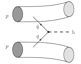
In Table 4 we collect the values of $\sigma[pp(\bar{q}q)\to\mathrm{h}]$ and $\mathcal{L}_{\bar{q}q}$ computed [104] for different quarks and setting $|a_{q}|^{2}+|b_{q}|^{2}=1$ in Eq. (91): this value of the couplings is obviously too large since it effectively corresponds, with respect to the SM, to the change $m_{j}/v\mapsto v/v$, but it allows for easy use.

	$\bar{d}d$		$\bar{u}u$		$\bar{s}s$		$\bar{c}c$
	$\mathcal{L}_{\bar{d}d}$	$\sigma$	$\mathcal{L}_{\bar{u}u}$	$\sigma$	$\mathcal{L}_{\bar{s}s}$	$\sigma$	$\mathcal{L}_{\bar{c}c}$	$\sigma$
8 TeV	14.56	16.60	21.53	24.53	4.41	5.02	2.65	3.01
13 TeV	74.57	29.17	105.28	41.18	27.70	10.84	17.92	7.01
14 TeV	95.49	31.53	133.90	44.21	36.46	12.04	23.83	7.87

Table 4: $\sigma[pp(\bar{q}q)\to\mathrm{h}]$ $(\times 10^{3})$ in pb and $\mathcal{L}_{\bar{q}q}(E^{2})$ $(\times 10^{3})$ for different $\bar{q}q$.

Consider, for illustration, that for the LHC at 8 TeV $\sigma[pp(\bar{u}u)\to\mathrm{h}]\sim 10$ pb: one can readily obtain

$$\sigma[pp(\bar{u}u)\to\mathrm{h}]\sim 10\text{ pb}\ \Leftrightarrow\ |a_{q}|^{2}+|b_{q}|^{2}\sim 7.3\times 10^{-5}\,.$$ (93)

Although considering $\sigma[pp(\bar{u}u)\to\mathrm{h}]\sim 10$ pb may be unrealistic (the total production cross section in Table 3 for 8 TeV is $\sim 22$ pb), from Eq. (93), $\Gamma(\mathrm{h}\to u\bar{u})\sim 1$ MeV: even if it is a significant contribution to the width $\Gamma(\mathrm{h})$, it might still be compatible with the overall pattern of Higgs signal strengths. To the knowledge of the authors, there are no dedicated analyses of $\bar{q}q\to\mathrm{h}$ ($q\neq b,t$) from which experimental input can be used in this manner. However, it is reasonable to expect that this kind of production potentially “contaminates” the analyses of gluon-gluon fusion: in that case, one should add all $\sigma[pp(\bar{q}q)\to\mathrm{h}]$ contributions for light $q$ to the gluon-gluon fusion cross section when analysing Higgs signal strengths. It is then clear that bounds more stringent than Eq. (93) would follow for the sum over all the different channels involved. The simple connection among the decays $\mathrm{h}\to\bar{q}q$ and the $\bar{q}q\to\mathrm{h}$ production mechanism – in the narrow width approximation – that follows from Eqs. (85) and (91), is

$$\frac{\sigma[pp(\bar{q}q)\to\mathrm{h}]\,/\,1\text{pb}}{\Gamma(\mathrm{h}\to\bar{q}q)\,/\,1\text{MeV}}=6.825\,\left(\frac{\text{TeV}}{E}\right)^{2}\left(\frac{\mathcal{L}_{\bar{q}q}(E)}{10^{3}}\right)\,,$$ (94)

which allows for easy comparison of the relative strengths of the constraints imposed by $\bar{q}q\to\mathrm{h}$ production and $\mathrm{h}\to\bar{q}q$ decay for light quarks $q$.

4.2.3 Constraints

The main source of experimental constraints that we use is the combined analysis of LHC-Run I data from the ATLAS and CMS collaborations in [91], which provides detailed information on (production) $\times$ (decay) of the 125 GeV Higgs $\mathrm{h}$ for

• production: ggF, VBF, associated $W\mathrm{h}Ç$, $Z\mathrm{h}$, and $tt\mathrm{h}$;

• decay: $\mathrm{h}\to\gamma\gamma$, $ZZ$, $WW$, $\tau\bar{\tau}$ and $b\bar{b}$.

Results from LHC-Run II in specific channels like (associated $V\mathrm{h}$) $\times$ ($\mathrm{h}\to b\bar{b}$) [105, 106], or (ggF+VBF) $\times$ ($\mathrm{h}\to\tau\bar{\tau}$) [107] are starting to improve over [91]. One should also consider off-shell (ggF+VBF)$\to\mathrm{h}^{(\ast)}\to WW^{(\ast)}$ constraints on the total width $\Gamma(\mathrm{h})$ [108], even if they are still weak [109, 110]. Finally, dedicated studies like [111, 112] put useful bounds on $\mathrm{h}\to\mu^{+}\mu^{-},e^{+}e^{-}$.

4.3 Electric dipole moments

As discussed at the end of section 2, non-real $\mathcal{N}_{\mathrm{f}}$ matrices are a source of CP violation in scalar-fermion interactions, which can induce electric dipole moments (EDMs). Consider for example an electron-Higgs coupling $\mathscr{L}_{\mathrm{h}ee}=-\mathrm{h}\,\bar{e}(a_{e}+ib_{e}\gamma_{5})e$; the one loop diagram in Figure 2 gives a contribution to the electron EDM $d_{e}$:

$$d_{e}=\frac{3m_{e}a_{e}b_{e}}{16\pi^{2}m_{\mathrm{h}}^{2}}\left(1+\mathcal{O}\left(\frac{m_{e}^{2}}{m_{\mathrm{h}}^{2}}\right)\right).$$ (95)

It is to be noticed that, for $a_{e}\sim b_{e}\sim m_{e}/v$, Eq. (95) gives $d_{e}\sim 10^{-34}$e$\cdot$cm. When $|a_{e}|$, $|b_{e}|\gg m_{e}/v$ are a priori allowed, up to the effect of other constraints, a significant enhancement in $d_{e}$ can be expected. For current experimental bounds $|d_{e}|<10^{-27}$e $\cdot$cm, considering only this contribution gives

$$a_{e}b_{e}<8\times 10^{-5},$$ (96)

or, with Eqs. (81)–(82) and neglecting $m_{e}$ with respect to $c_{\beta\alpha}n_{e}$,

$$c_{\beta\alpha}^{2}\text{Re}(n_{e})\text{Im}(n_{e})<5\text{ GeV}^{2}.$$ (97)

Anticipating results from section 4.4, in particular Figure 4(g), it is clear that the bounds imposed by the LHC results are more stringent than Eq. (97). It should also be noticed that including contributions analog to Figure 2 with $\mathrm{h}\to\mathrm{H},\mathrm{A}$, gives

$$\text{Re}(n_{e})\text{Im}(n_{e})\left(c_{\beta\alpha}^{2}+s_{\beta\alpha}^{2}\frac{m_{\mathrm{h}}^{2}}{m_{\mathrm{H}}^{2}}+\frac{m_{\mathrm{h}}^{2}}{m_{\mathrm{A}}^{2}}\right)<5\text{ GeV}^{2},$$ (98)

and does not change this conclusion. Furthermore, one loop contributions with virtual $\mathrm{H}^{\pm}$ and neutrinos are suppressed.

Figure 2: $\mathrm{h}$ mediated contribution to $d_{e}$ at one loop.

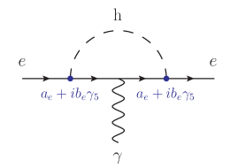
It is well known that two loop “Barr-Zee” [113, 114, 115, 116, 117, 118] contributions can be significant: studies such as [119, 120] address such constraints on CP violating Higgs-fermion couplings. However, those contributions involve different $n_{f}$ couplings simultaneously, together with the masses of the different scalars, preventing a simple translation into bounds on a single parameter. It is to be noticed too that cancellations among different diagrams in that class may occur [67, 121]. Including such kind of analysis is beyond the scope of this work; in any case one should keep in mind that the analysis of EDMs may have some impact on the results of section 4.4. The previous discussion also applies to the EDMs of the $u$ and $d$ quarks and the experimental constraints that the neutron EDM bounds impose, including, in addition, the impact of QCD effects [122].

4.4 Analysis

With the deviations with respect to the SM of the couplings of $\mathrm{h}$ and their implications for decays and production mechanisms, one can impose the experimental constraints of section 4.2.3 and explore the allowed values of $c_{\beta\alpha}$ and the gFC parameters $n_{f}$ in Eq. (38). For the results presented in the following we consider the most conservative situation, i.e. all parameters are free to vary simultaneously. Compared to restricted situations where not all parameters are considered simultaneously, this offers a safer interpretation of excluded regions (they are excluded whatever the values of the parameters not displayed) at the price, of course, of larger allowed regions.
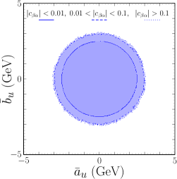
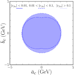
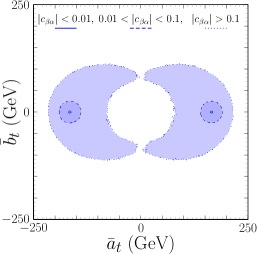
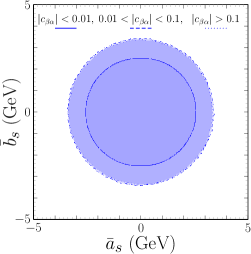
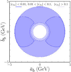
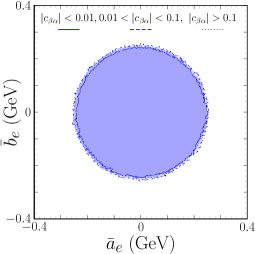
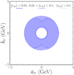
Figure 3 shows $n_{f}$ vs. $c_{\beta\alpha}$ for all quarks and leptons. Some comments are in order.

(a) $u$

(b) $c$

(c) $t$

(d) $d$

(e) $s$

(f) $b$

(g) $e$

(h) $\mu$

(i) $\tau$

Figure 3: $|n_{f}|$ vs. $c_{\beta\alpha}$ for the different fermions $f$; darker to lighter regions correspond to 68, 95 and 99% CL.

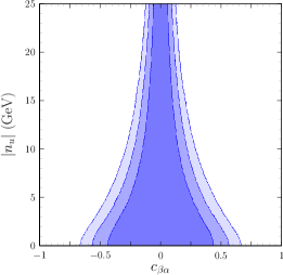
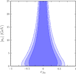
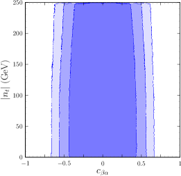
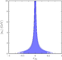
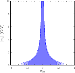
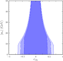
• As expected, for $c_{\beta\alpha}\to 0$, the constraints on $n_{f}$ disappear.

• For $u$, $c$, $d$ and $s$ quarks, the allowed regions are almost identical, as one could anticipate from their irrelevant role, within the SM, in the available production $\times$ decay Higgs signal strengths. The corresponding $n_{f}$’s appear to be effectively limited by the contributions to the Higgs width.

• Surprisingly, the allowed size of $|n_{t}|$ appears to be independent of $c_{\beta\alpha}$: this will be discussed in connection with Fig. 4(c) below.

• The $n_{b}$ and $n_{\tau}$ cases are also similar, with allowed regions differing from the $u$, $c$, $d$, $s$ cases for $|n_{q}|$’s below 10-15 GeV and not small $c_{\beta\alpha}$.

• For $n_{e}$ and $n_{\mu}$, the allowed regions are much more constrained owing to the bounds set by dedicated $pp\to\mathrm{h}\to$ $e^{+}e^{-}$, $\mu^{+}\mu^{-}$ analyses such as [111, 112].

Although Fig. 3 shows absolute bounds on $|n_{f}|$’s, it does not give information on $\arg(n_{f})$’s and cannot be directly read in terms of the scalar and pseudoscalar couplings of $\mathrm{h}$ in Eqs. (81)–(82). Considering that, Figure 4 shows $\bar{b}_{f}$ vs $\bar{a}_{f}$ with

$$\bar{a}_{f}\equiv s_{\beta\alpha}m_{f}+c_{\beta\alpha}\text{Re}(n_{f}),\quad\bar{b}_{f}=c_{\beta\alpha}\text{Im}(n_{f})\,.$$ (99)

Furthermore, to maintain some information on $c_{\beta\alpha}$, allowed regions corresponding to $|c_{\beta\alpha}|<0.01$, to $0.01<|c_{\beta\alpha}|<0.1$ and to $0.1<|c_{\beta\alpha}|$ are displayed. One can notice that

• for the first and second fermion generations, there is no dependence on $\arg(n_{f})$, since only decays, with rates proportional to $|\bar{a}_{f}|^{2}+|\bar{b}_{f}|^{2}$, are relevant. For quarks, the allowed region for $|c_{\beta\alpha}|<0.01$ is smaller: this is simply due to the perturbativity requirement in Eq. (79).

• For the top quark, two separate regions are allowed: this is also expected since independent sign changes in both $\bar{a}_{t}$ and $\bar{b}_{t}$ (together with sign changes in $c_{\beta\alpha}$, $s_{\beta\alpha}$) do not alter the predictions. For $|c_{\beta\alpha}|<0.01$ the allowed regions are quite reduced and placed around $(\bar{a}_{t},\bar{b}_{t})=(\pm m_{t},0)$; with $0.01<|c_{\beta\alpha}|<0.1$ their size increases and only for $|c_{\beta\alpha}|>0.1$ the interplay of (i) pseudoscalar contributions to $gg\to\mathrm{h}$ and $\mathrm{h}\to\gamma\gamma$, and (ii) $W$-top(scalar) interference in $\mathrm{h}\to\gamma\gamma$ gives rise to larger regions.

• For $b$ and $\tau$, the regions for not too small mixing, $|c_{\beta\alpha}|>0.01$, are ring-shaped; $m_{b}$ and $m_{\tau}$ set the radii of such regions, as could be expected from the agreement of $\mathrm{h}\to b\bar{b}$ and $\mathrm{h}\to\tau\bar{\tau}$ signal strengths with SM expectations. For small mixing, $|c_{\beta\alpha}|<0.01$, the perturbativity requirement on $|n_{b}|$, $|n_{\tau}|$ limits the allowed departure from $(\bar{a}_{f},\bar{b}_{f})=(\pm m_{f},0)$, giving in fact, for the $b$ case, two disjoint patches.

(a) $u$

(b) $c$

(c) $t$

(d) $d$

(e) $s$

(f) $b$

(g) $e$

(h) $\mu$

(i) $\tau$

Figure 4: Allowed regions at 99% CL for pseudoscalar vs. scalar couplings for the different fermions $f$ with $\mathscr{L}_{\mathrm{h}\bar{f}f}=-\frac{\mathrm{h}}{v}\bar{f}(\bar{a}_{f}+i\bar{b}_{f}\gamma_{5})f$.

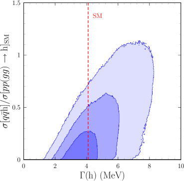
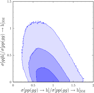
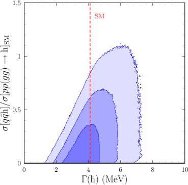
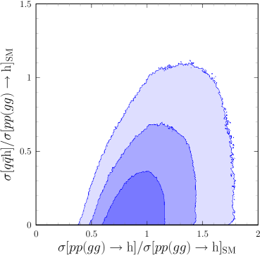
To close this section we recall the discussion on $\bar{q}q\to\mathrm{h}$ production in section 4.2.2: as commented there, values of $n_{f}$ in agreement with the SM-like Higgs signal strengths could potentially give production cross sections not far from the dominating SM ones. Figure 5 shows

$$\frac{\sigma[q\bar{q}\mathrm{h}]}{\sigma[pp(gg)\to\mathrm{h}]_{\rm SM}}\equiv\left(\sum_{q=u,c,d,s}\sigma[pp(q\bar{q})\to\mathrm{h}]\right){\Big{/}}\sigma[pp(gg)\to\mathrm{h}]_{\rm SM},$$ (100)

vs. the total Higgs width and vs. the gluon-gluon fusion production cross section in two different analyses: in Figures 5(a) and 5(b), $\sigma[q\bar{q}\mathrm{h}]$ is added to the ggF production cross section, while in Figures 5(c) and 5(d) it is not (and therefore, in the analysis, it does not affect directly observables constrained by experiment). Comparing 5(a)-5(b) with 5(c)-5(d), one can notice that the constraints from Higgs signal strengths are able to bound the size of $\sigma[q\bar{q}\mathrm{h}]$, even if there is room for an overall $q\bar{q}\to\mathrm{h}$ cross section which is quite sizable, not far from the complete SM Higgs production cross section. Furthermore, when $\sigma[q\bar{q}\mathrm{h}]$ is added to the ggF production cross section, the agreement with the observed Higgs signal strengths allows for a smaller amount of $q\bar{q}\to\mathrm{h}$, and, for sizable $q\bar{q}\to\mathrm{h}$, it is achieved at the cost of (i) reducing the ggF production cross section and (ii) increasing the total width $\Gamma(\mathrm{h})$, as the shape of the allowed regions in Figures 5(a) and 5(b) shows. For the results in Figures 3 and 4, the bounds on the the different $\bar{a}_{f}$, $\bar{b}_{f}$ do not differ in both analyses. It should be finally mentioned that, in connection with the previous comments and the size of $\sigma[pp(q\bar{q})\to\mathrm{h}]$, it might be interesting to analyse, for the remaining neutral scalars $\mathrm{H}$ and $\mathrm{A}$, the cross sections for $pp(q\bar{q})\to\mathrm{H},\mathrm{A}$ at the LHC.

(a) ${\sigma[q\bar{q}\mathrm{h}]}$ vs. $\Gamma(\mathrm{h})$, ${\sigma[q\bar{q}\mathrm{h}]\subset\text{ ggF}}$.

(b) ${\sigma[q\bar{q}\mathrm{h}]}$ vs. ${\sigma[pp(gg)\to\mathrm{h}]}$, ${\sigma[q\bar{q}\mathrm{h}]\subset\text{ ggF}}$

(c) ${\sigma[q\bar{q}\mathrm{h}]}$ vs. $\Gamma(\mathrm{h})$, ${\sigma[q\bar{q}\mathrm{h}]\not\subset\text{ ggF}}$

(d) ${\sigma[q\bar{q}\mathrm{h}]}$ vs. ${\sigma[pp(gg)\to\mathrm{h}]}$, ${\sigma[q\bar{q}\mathrm{h}]\not\subset\text{ ggF}}$

Figure 5: Effect of including $q\bar{q}\to\mathrm{h}$ production in ggF in analyses of Higgs signal strengths; darker to lighter regions correspond to 68, 95 and 99% CL.

Conclusions

In this paper we analyse the question of general Flavour Conservation in extensions of the SM with additional scalar doublets, in particular the 2HDM. The effect of the one loop Renomalization Group Evolution of the Yukawa coupling matrices on gFC scenarios is discussed in detail. In particular it is to be stressed that in the absence of Yukawa couplings with right-handed neutrinos, gFC in the lepton sector is stable. For the quark sector, some one loop RGE stable scenarios are discussed, including the case of a Cabibbo-like quark mixing matrix. At a phenomenological level, we discuss the constraints that existing data on flavour conserving processes, in particular the ones related to the Higgs, impose on the parameters describing gFC in the different fermion sectors, including a detailed numerical analysis of that parameter space. Direct $q\bar{q}\to\mathrm{h}$ production is also considered in detail: although it is completely negligible in the SM, that might not be the case in scenarios such as 2HDM, and it may even be relevant for the production of the additional non-SM neutral scalars.

Appendix A RGE details

The analysis of the RGE of the quark Yukawa couplings and the stability of the gFC scenario in Eq. (38) has been presented in detail for the set $\{\Gamma^{\phantom{\dagger}}_{\alpha}\Gamma^{\dagger}_{\beta}\}$ in section 3.1 and 3.2. We reproduce in this appendix the equations relevant for $\{\Gamma^{\phantom{\dagger}}_{\alpha}\Gamma^{\dagger}_{\beta}\}$ and also for $\{\Gamma^{\dagger}_{\alpha}\Gamma^{\phantom{\dagger}}_{\beta}\}$, $\{\Delta^{\phantom{\dagger}}_{\alpha}\Delta^{\dagger}_{\beta}\}$ and $\{\Delta^{\dagger}_{\alpha}\Delta^{\phantom{\dagger}}_{\beta}\}$, omitted for conciseness in section 3. In correspondence with Eqs. (46), (47) and (48),

$$\mathcal{D}(\Gamma^{\phantom{\dagger}}_{\alpha}\Gamma^{\dagger}_{\beta}) =f^{\rm[d_{L}]}_{\alpha\beta}(\Gamma)+g^{\rm[d_{L}]}_{\alpha\beta}(\Gamma,\Delta)\,,\quad\mathcal{D}(\Delta^{\phantom{\dagger}}_{\alpha}\Delta^{\dagger}_{\beta}) =f^{\rm[u_{L}]}_{\alpha\beta}(\Delta)+g^{\rm[u_{L}]}_{\alpha\beta}(\Gamma,\Delta)\,,$$

$$\mathcal{D}(\Gamma^{\dagger}_{\alpha}\Gamma^{\phantom{\dagger}}_{\beta}) =f^{\rm[d_{R}]}_{\alpha\beta}(\Gamma)+g^{\rm[d_{R}]}_{\alpha\beta}(\Gamma,\Delta)\,,\quad\mathcal{D}(\Delta^{\dagger}_{\alpha}\Delta^{\phantom{\dagger}}_{\beta}) =f^{\rm[u_{R}]}_{\alpha\beta}(\Delta)+g^{\rm[u_{R}]}_{\alpha\beta}(\Gamma,\Delta)\,,$$ (101)

with

$$f^{\rm[d_{L}]}_{\alpha\beta}(\Gamma)=2a_{d}\Gamma^{\phantom{\dagger}}_{\alpha}\Gamma^{\dagger}_{\beta}+\sum_{\rho=1}^{n=2}\left[T^{d}_{\alpha,\rho}\Gamma^{\phantom{\dagger}}_{\rho}\Gamma^{\dagger}_{\beta}+T^{d\ast}_{\beta,\rho}\Gamma^{\phantom{\dagger}}_{\alpha}\Gamma^{\dagger}_{\rho}\right]+2\Gamma^{\phantom{\dagger}}_{\alpha}{\Large\Gamma}_{R}\Gamma^{\dagger}_{\beta}+\frac{1}{2}{\Large\Gamma}_{L}\Gamma^{\phantom{\dagger}}_{\alpha}\Gamma^{\dagger}_{\beta}+\frac{1}{2}\Gamma^{\phantom{\dagger}}_{\alpha}\Gamma^{\dagger}_{\beta}{\Large\Gamma}_{L}\,,$$

$$g^{\rm[d_{L}]}_{\alpha\beta}(\Gamma,\Delta)=\frac{1}{2}{\large\Delta}_{L}\Gamma^{\phantom{\dagger}}_{\alpha}\Gamma^{\dagger}_{\beta}+\frac{1}{2}\Gamma^{\phantom{\dagger}}_{\alpha}\Gamma^{\dagger}_{\beta}{\large\Delta}_{L}-2\sum_{\rho=1}^{n=2}\left[\Delta^{\phantom{\dagger}}_{\rho}\Delta^{\dagger}_{\alpha}\Gamma^{\phantom{\dagger}}_{\rho}\Gamma^{\dagger}_{\beta}+\Gamma^{\phantom{\dagger}}_{\alpha}\Gamma^{\dagger}_{\rho}\Delta^{\phantom{\dagger}}_{\beta}\Delta^{\dagger}_{\rho}\right],$$ (102)

$$f^{\rm[d_{R}]}_{\alpha\beta}(\Gamma)=2a_{d}\Gamma^{\dagger}_{\alpha}\Gamma^{\phantom{\dagger}}_{\beta}+\sum_{\rho=1}^{n=2}\left[T^{d\ast}_{\alpha,\rho}\Gamma^{\dagger}_{\rho}\Gamma^{\phantom{\dagger}}_{\beta}+T^{d}_{\beta,\rho}\Gamma^{\dagger}_{\alpha}\Gamma^{\phantom{\dagger}}_{\rho}\right]+\Gamma^{\dagger}_{\alpha}{\Large\Gamma}_{L}\Gamma^{\phantom{\dagger}}_{\beta}+{\Large\Gamma}_{R}\Gamma^{\dagger}_{\alpha}\Gamma^{\phantom{\dagger}}_{\beta}+\Gamma^{\dagger}_{\alpha}\Gamma^{\phantom{\dagger}}_{\beta}{\Large\Gamma}_{R}\,,$$

$$g^{\rm[d_{R}]}_{\alpha\beta}(\Gamma,\Delta)=\Gamma^{\dagger}_{\alpha}{\large\Delta}_{L}\Gamma^{\phantom{\dagger}}_{\beta}-2\sum_{\rho=1}^{n=2}\left[\Gamma^{\dagger}_{\rho}\Delta^{\phantom{\dagger}}_{\alpha}\Delta^{\dagger}_{\rho}\Gamma^{\phantom{\dagger}}_{\beta}+\Gamma^{\dagger}_{\alpha}\Delta^{\phantom{\dagger}}_{\rho}\Delta^{\dagger}_{\beta}\Gamma^{\phantom{\dagger}}_{\rho}\right],$$ (103)

$$f^{\rm[u_{L}]}_{\alpha\beta}(\Delta)=2a_{u}\Delta^{\phantom{\dagger}}_{\alpha}\Delta^{\dagger}_{\beta}+\sum_{\rho=1}^{n=2}\left[T^{u}_{\alpha,\rho}\Delta^{\phantom{\dagger}}_{\rho}\Delta^{\dagger}_{\beta}+T^{d\ast}_{\beta,\rho}\Delta^{\phantom{\dagger}}_{\alpha}\Delta^{\dagger}_{\rho}\right]+2\Delta^{\phantom{\dagger}}_{\alpha}{\large\Delta}_{R}\Delta^{\dagger}_{\beta}+\frac{1}{2}{\large\Delta}_{L}\Delta^{\phantom{\dagger}}_{\alpha}\Delta^{\dagger}_{\beta}+\frac{1}{2}\Delta^{\phantom{\dagger}}_{\alpha}\Delta^{\dagger}_{\beta}{\large\Delta}_{L}\,,$$

$$g^{\rm[u_{L}]}_{\alpha\beta}(\Gamma,\Delta)=\frac{1}{2}{\Large\Gamma}_{L}\Delta^{\phantom{\dagger}}_{\alpha}\Delta^{\dagger}_{\beta}+\frac{1}{2}\Delta^{\phantom{\dagger}}_{\alpha}\Delta^{\dagger}_{\beta}{\Large\Gamma}_{L}-2\sum_{\rho=1}^{n=2}\left[\Gamma^{\phantom{\dagger}}_{\rho}\Gamma^{\dagger}_{\alpha}\Delta^{\phantom{\dagger}}_{\rho}\Delta^{\dagger}_{\beta}+\Delta^{\phantom{\dagger}}_{\alpha}\Delta^{\dagger}_{\rho}\Gamma^{\phantom{\dagger}}_{\beta}\Gamma^{\dagger}_{\rho}\right],$$ (104)

and

$$f^{\rm[u_{R}]}_{\alpha\beta}(\Gamma)=2a_{u}\Delta^{\dagger}_{\alpha}\Delta^{\phantom{\dagger}}_{\beta}+\sum_{\rho=1}^{n=2}\left[T^{u\ast}_{\alpha,\rho}\Delta^{\dagger}_{\rho}\Delta^{\phantom{\dagger}}_{\beta}+T^{u}_{\beta,\rho}\Delta^{\dagger}_{\alpha}\Delta^{\phantom{\dagger}}_{\rho}\right]+\Delta^{\dagger}_{\alpha}{\large\Delta}_{L}\Delta^{\phantom{\dagger}}_{\beta}+{\large\Delta}_{R}\Delta^{\dagger}_{\alpha}\Delta^{\phantom{\dagger}}_{\beta}+\Delta^{\dagger}_{\alpha}\Delta^{\phantom{\dagger}}_{\beta}{\large\Delta}_{R}\,,$$

$$g^{\rm[u_{R}]}_{\alpha\beta}(\Gamma,\Delta)=\Delta^{\dagger}_{\alpha}{\Large\Gamma}_{L}\Delta^{\phantom{\dagger}}_{\beta}-2\sum_{\rho=1}^{n=2}\left[\Delta^{\dagger}_{\rho}\Gamma^{\phantom{\dagger}}_{\alpha}\Gamma^{\dagger}_{\rho}\Delta^{\phantom{\dagger}}_{\beta}+\Delta^{\dagger}_{\alpha}\Gamma^{\phantom{\dagger}}_{\rho}\Gamma^{\dagger}_{\beta}\Delta^{\phantom{\dagger}}_{\rho}\right].$$ (105)

The RGE of the commutation relations of Eq. (37) reads

$$\mathcal{D}\left[\Gamma^{\phantom{\dagger}}_{\alpha}\Gamma^{\dagger}_{\beta}\,,\,\Gamma^{\phantom{\dagger}}_{\gamma}\Gamma^{\dagger}_{\delta}\right] =\left[g^{\rm[d_{L}]}_{\alpha\beta}(\Gamma,\Delta)\,,\,\Gamma^{\phantom{\dagger}}_{\gamma}\Gamma^{\dagger}_{\delta}\right]+\left[\Gamma^{\phantom{\dagger}}_{\alpha}\Gamma^{\dagger}_{\beta}\,,\,g^{\rm[d_{L}]}_{\gamma\delta}(\Gamma,\Delta)\right]\,,$$

$$\mathcal{D}\left[\Gamma^{\dagger}_{\alpha}\Gamma^{\phantom{\dagger}}_{\beta}\,,\,\Gamma^{\dagger}_{\gamma}\Gamma^{\phantom{\dagger}}_{\delta}\right] =\left[g^{\rm[d_{R}]}_{\alpha\beta}(\Gamma,\Delta)\,,\,\Gamma^{\dagger}_{\gamma}\Gamma^{\phantom{\dagger}}_{\delta}\right]+\left[\Gamma^{\dagger}_{\alpha}\Gamma^{\phantom{\dagger}}_{\beta}\,,\,g^{\rm[d_{R}]}_{\gamma\delta}(\Gamma,\Delta)\right]\,,$$

$$\mathcal{D}\left[\Delta^{\phantom{\dagger}}_{\alpha}\Delta^{\dagger}_{\beta}\,,\,\Delta^{\phantom{\dagger}}_{\gamma}\Delta^{\dagger}_{\delta}\right] =\left[g^{\rm[u_{L}]}_{\alpha\beta}(\Gamma,\Delta)\,,\,\Delta^{\phantom{\dagger}}_{\gamma}\Delta^{\dagger}_{\delta}\right]+\left[\Delta^{\phantom{\dagger}}_{\alpha}\Delta^{\dagger}_{\beta}\,,\,g^{\rm[u_{L}]}_{\gamma\delta}(\Gamma,\Delta)\right]\,,$$

$$\mathcal{D}\left[\Delta^{\dagger}_{\alpha}\Delta^{\phantom{\dagger}}_{\beta}\,,\,\Delta^{\dagger}_{\gamma}\Delta^{\phantom{\dagger}}_{\delta}\right] =\left[g^{\rm[u_{R}]}_{\alpha\beta}(\Gamma,\Delta)\,,\,\Delta^{\dagger}_{\gamma}\Gamma^{\phantom{\dagger}}_{\delta}\right]+\left[\Delta^{\dagger}_{\alpha}\Delta^{\phantom{\dagger}}_{\beta}\,,\,g^{\rm[u_{R}]}_{\gamma\delta}(\Gamma,\Delta)\right]\,,$$ (106)

which, following the discussion in section 3.2, lead to (summation over $h=1,2$ understood)

$$\{d_{L}\}\equiv\frac{v^{2}}{2} U_{{\rm d_{L}}}^{\dagger}\left(\mathcal{D}\left[Y^{0\phantom{\dagger}}_{{\rm[d]}i}Y^{0\dagger}_{{\rm[d]}j}\,,\,Y^{0\phantom{\dagger}}_{{\rm[d]}k}Y^{0\dagger}_{{\rm[d]}l}\right]\right)U_{{\rm d_{L}}}^{\phantom{\dagger}}=$$ (107)

$$Y^{\phantom{\dagger}}_{{\rm[d]}i}Y^{\dagger}_{{\rm[d]}j}\,V^{\dagger}Y^{\phantom{\dagger}}_{{\rm[u]}h}Y^{\dagger}_{{\rm[u]}h}V\,Y^{\phantom{\dagger}}_{{\rm[d]}k}Y^{\dagger}_{{\rm[d]}l}-Y^{\phantom{\dagger}}_{{\rm[d]}k}Y^{\dagger}_{{\rm[d]}l}\,V^{\dagger}Y^{\phantom{\dagger}}_{{\rm[u]}h}Y^{\dagger}_{{\rm[u]}h}V\,Y^{\phantom{\dagger}}_{{\rm[d]}i}Y^{\dagger}_{{\rm[d]}j}$$

$$-2\left[V^{\dagger}Y^{\phantom{\dagger}}_{{\rm[u]}h}Y^{\dagger}_{{\rm[u]}i}V\,,\,Y^{\phantom{\dagger}}_{{\rm[d]}k}Y^{\dagger}_{{\rm[d]}l}\right]Y^{\phantom{\dagger}}_{{\rm[d]}h}Y^{\dagger}_{{\rm[d]}j}-2Y^{\phantom{\dagger}}_{{\rm[d]}i}Y^{\dagger}_{{\rm[d]}h}\left[V^{\dagger}Y^{\phantom{\dagger}}_{{\rm[u]}j}Y^{\dagger}_{{\rm[u]}h}V\,,\,Y^{\phantom{\dagger}}_{{\rm[d]}k}Y^{\dagger}_{{\rm[d]}l}\right]$$

$$+2\left[V^{\dagger}Y^{\phantom{\dagger}}_{{\rm[u]}h}Y^{\dagger}_{{\rm[u]}k}V\,,\,Y^{\phantom{\dagger}}_{{\rm[d]}i}Y^{\dagger}_{{\rm[d]}j}\right]Y^{\phantom{\dagger}}_{{\rm[d]}h}Y^{\dagger}_{{\rm[d]}l}+2Y^{\phantom{\dagger}}_{{\rm[d]}k}Y^{\dagger}_{{\rm[d]}h}\left[V^{\dagger}Y^{\phantom{\dagger}}_{{\rm[u]}l}Y^{\dagger}_{{\rm[u]}h}V\,,\,Y^{\phantom{\dagger}}_{{\rm[d]}i}Y^{\dagger}_{{\rm[d]}j}\right],$$

$$\{d_{R}\}\equiv\frac{v^{2}}{2} U_{{\rm d_{R}}}^{\dagger}\left(\mathcal{D}\left[Y^{0\dagger}_{{\rm[d]}i}Y^{0\phantom{\dagger}}_{{\rm[d]}j}\,,\,Y^{0\dagger}_{{\rm[d]}k}Y^{0\phantom{\dagger}}_{{\rm[d]}l}\right]\right)U_{{\rm d_{R}}}^{\phantom{\dagger}}=$$ (108)

$$\left[Y^{\dagger}_{{\rm[d]}i}\,V^{\dagger}Y^{\phantom{\dagger}}_{{\rm[u]}h}Y^{\dagger}_{{\rm[u]}h}V\,Y^{\phantom{\dagger}}_{{\rm[d]}j}\,,\,Y^{\dagger}_{{\rm[d]}k}Y^{\phantom{\dagger}}_{{\rm[d]}l}\right]-\left[Y^{\dagger}_{{\rm[d]}k}\,V^{\dagger}Y^{\phantom{\dagger}}_{{\rm[u]}h}Y^{\dagger}_{{\rm[u]}h}V\,Y^{\phantom{\dagger}}_{{\rm[d]}l}\,,\,Y^{\dagger}_{{\rm[d]}i}Y^{\phantom{\dagger}}_{{\rm[d]}j}\right]$$

$$-2\left[Y^{\dagger}_{{\rm[d]}h}\,V^{\dagger}Y^{\phantom{\dagger}}_{{\rm[u]}i}Y^{\dagger}_{{\rm[u]}h}V\,Y^{\phantom{\dagger}}_{{\rm[d]}j}\,,\,Y^{\dagger}_{{\rm[d]}k}Y^{\phantom{\dagger}}_{{\rm[d]}l}\right]-2\left[Y^{\dagger}_{{\rm[d]}i}\,V^{\dagger}Y^{\phantom{\dagger}}_{{\rm[u]}h}Y^{\dagger}_{{\rm[u]}j}V\,Y^{\phantom{\dagger}}_{{\rm[d]}h}\,,\,Y^{\dagger}_{{\rm[d]}k}Y^{\phantom{\dagger}}_{{\rm[d]}l}\right]$$

$$+2\left[Y^{\dagger}_{{\rm[d]}h}\,V^{\dagger}Y^{\phantom{\dagger}}_{{\rm[u]}k}Y^{\dagger}_{{\rm[u]}h}V\,Y^{\phantom{\dagger}}_{{\rm[d]}l}\,,\,Y^{\dagger}_{{\rm[d]}i}Y^{\phantom{\dagger}}_{{\rm[d]}j}\right]+2\left[Y^{\dagger}_{{\rm[d]}k}\,V^{\dagger}Y^{\phantom{\dagger}}_{{\rm[u]}h}Y^{\dagger}_{{\rm[u]}l}V\,Y^{\phantom{\dagger}}_{{\rm[d]}h}\,,\,Y^{\dagger}_{{\rm[d]}i}Y^{\phantom{\dagger}}_{{\rm[d]}j}\right],$$

$$\{u_{L}\}\equiv\frac{v^{2}}{2} U_{{\rm u_{L}}}^{\dagger}\left(\mathcal{D}\left[Y^{0\phantom{\dagger}}_{{\rm[u]}i}Y^{0\dagger}_{{\rm[u]}j}\,,\,Y^{0\phantom{\dagger}}_{{\rm[u]}k}Y^{0\dagger}_{{\rm[u]}l}\right]\right)U_{{\rm u_{L}}}^{\phantom{\dagger}}=$$ (109)

$$Y^{\phantom{\dagger}}_{{\rm[u]}i}Y^{\dagger}_{{\rm[u]}j}\,VY^{\phantom{\dagger}}_{{\rm[d]}h}Y^{\dagger}_{{\rm[d]}h}V^{\dagger}\,Y^{\phantom{\dagger}}_{{\rm[u]}k}Y^{\dagger}_{{\rm[u]}l}-Y^{\phantom{\dagger}}_{{\rm[u]}k}Y^{\dagger}_{{\rm[u]}l}\,VY^{\phantom{\dagger}}_{{\rm[d]}h}Y^{\dagger}_{{\rm[d]}h}V^{\dagger}\,Y^{\phantom{\dagger}}_{{\rm[u]}i}Y^{\dagger}_{{\rm[u]}j}$$

$$-2\left[VY^{\phantom{\dagger}}_{{\rm[d]}h}Y^{\dagger}_{{\rm[d]}i}V^{\dagger}\,,\,Y^{\phantom{\dagger}}_{{\rm[u]}k}Y^{\dagger}_{{\rm[u]}l}\right]Y^{\phantom{\dagger}}_{{\rm[u]}h}Y^{\dagger}_{{\rm[u]}j}-2Y^{\phantom{\dagger}}_{{\rm[u]}i}Y^{\dagger}_{{\rm[u]}h}\left[VY^{\phantom{\dagger}}_{{\rm[d]}j}Y^{\dagger}_{{\rm[d]}h}V^{\dagger}\,,\,Y^{\phantom{\dagger}}_{{\rm[u]}k}Y^{\dagger}_{{\rm[u]}l}\right]$$

$$+2\left[VY^{\phantom{\dagger}}_{{\rm[d]}h}Y^{\dagger}_{{\rm[d]}k}V^{\dagger}\,,\,Y^{\phantom{\dagger}}_{{\rm[u]}i}Y^{\dagger}_{{\rm[u]}j}\right]Y^{\phantom{\dagger}}_{{\rm[u]}h}Y^{\dagger}_{{\rm[u]}l}+2Y^{\phantom{\dagger}}_{{\rm[u]}k}Y^{\dagger}_{{\rm[u]}h}\left[VY^{\phantom{\dagger}}_{{\rm[d]}l}Y^{\dagger}_{{\rm[d]}h}V^{\dagger}\,,\,Y^{\phantom{\dagger}}_{{\rm[u]}i}Y^{\dagger}_{{\rm[u]}j}\right],$$

and

$$\{u_{R}\}\equiv\frac{v^{2}}{2} U_{{\rm u_{R}}}^{\dagger}\left(\mathcal{D}\left[Y^{0\dagger}_{{\rm[u]}i}Y^{0\phantom{\dagger}}_{{\rm[u]}j}\,,\,Y^{0\dagger}_{{\rm[u]}k}Y^{0\phantom{\dagger}}_{{\rm[u]}l}\right]\right)U_{{\rm u_{R}}}^{\phantom{\dagger}}=$$ (110)

$$\left[Y^{\dagger}_{{\rm[u]}i}\,VY^{\phantom{\dagger}}_{{\rm[d]}h}Y^{\dagger}_{{\rm[d]}h}V^{\dagger}\,Y^{\phantom{\dagger}}_{{\rm[u]}j}\,,\,Y^{\dagger}_{{\rm[u]}k}Y^{\phantom{\dagger}}_{{\rm[u]}l}\right]-\left[Y^{\dagger}_{{\rm[u]}k}\,VY^{\phantom{\dagger}}_{{\rm[d]}h}Y^{\dagger}_{{\rm[d]}h}V^{\dagger}\,Y^{\phantom{\dagger}}_{{\rm[u]}l}\,,\,Y^{\dagger}_{{\rm[u]}i}Y^{\phantom{\dagger}}_{{\rm[u]}j}\right]$$

$$-2\left[Y^{\dagger}_{{\rm[u]}h}\,VY^{\phantom{\dagger}}_{{\rm[d]}i}Y^{\dagger}_{{\rm[d]}h}V^{\dagger}\,Y^{\phantom{\dagger}}_{{\rm[u]}j}\,,\,Y^{\dagger}_{{\rm[u]}k}Y^{\phantom{\dagger}}_{{\rm[u]}l}\right]-2\left[Y^{\dagger}_{{\rm[u]}i}\,VY^{\phantom{\dagger}}_{{\rm[d]}h}Y^{\dagger}_{{\rm[d]}j}V^{\dagger}\,Y^{\phantom{\dagger}}_{{\rm[u]}h}\,,\,Y^{\dagger}_{{\rm[u]}k}Y^{\phantom{\dagger}}_{{\rm[u]}l}\right]$$

$$+2\left[Y^{\dagger}_{{\rm[u]}h}\,VY^{\phantom{\dagger}}_{{\rm[d]}k}Y^{\dagger}_{{\rm[d]}h}V^{\dagger}\,Y^{\phantom{\dagger}}_{{\rm[u]}l}\,,\,Y^{\dagger}_{{\rm[u]}i}Y^{\phantom{\dagger}}_{{\rm[u]}j}\right]+2\left[Y^{\dagger}_{{\rm[u]}k}\,VY^{\phantom{\dagger}}_{{\rm[d]}h}Y^{\dagger}_{{\rm[d]}l}V^{\dagger}\,Y^{\phantom{\dagger}}_{{\rm[u]}h}\,,\,Y^{\dagger}_{{\rm[u]}i}Y^{\phantom{\dagger}}_{{\rm[u]}j}\right].$$

In order to compute the matrix elements of Eqs. (107)–(110), we notice that

$$\left(\left[V^{\dagger}Y^{\phantom{\dagger}}_{{\rm[u]}i}Y^{\dagger}_{{\rm[u]}j}V\,,\,Y^{\dagger}_{{\rm[d]}k}Y^{\phantom{\dagger}}_{{\rm[d]}l}\right]\right)_{ab}=\sum_{q=1}^{3}{V_{qa}^{\ast}}{V_{qb}^{\phantom{\ast}}}y^{{\rm u}\phantom{\ast}}_{{i},q}y^{{\rm u}\ast}_{{j},q}(y^{{\rm d}\ast}_{{k},b}y^{{\rm d}\phantom{\ast}}_{{l},b}-y^{{\rm d}\ast}_{{k},a}y^{{\rm d}\phantom{\ast}}_{{l},a}),$$ (111)

and

$$\left(\left[VY^{\phantom{\dagger}}_{{\rm[d]}i}Y^{\dagger}_{{\rm[d]}j}V^{\dagger}\,,\,Y^{\phantom{\dagger}}_{{\rm[u]}k}Y^{\dagger}_{{\rm[u]}l}\right]\right)_{ab}=\sum_{q=1}^{3}{V_{aq}^{\phantom{\ast}}}{V_{bq}^{\ast}}y^{{\rm d}\phantom{\ast}}_{{i},q}y^{{\rm d}\ast}_{{j},q}(y^{{\rm u}\phantom{\ast}}_{{k},b}y^{{\rm u}\ast}_{{l},b}-y^{{\rm u}\phantom{\ast}}_{{k},a}y^{{\rm u}\ast}_{{l},a}).$$ (112)

Then, with the parameters in Eq. (62), the matrix elements $(a,b)$ of Eqs. (107)–(110) read

$$\{d_{L}\}_{ab}=\sum_{q=1}^{3}\sum_{{\rm h}=1}^{n=2}{V_{qa}^{\ast}}{V_{qb}^{\phantom{\ast}}}\Big{\{} |y^{{\rm u}\phantom{\ast}}_{{h},q}|^{2}\left(y^{{\rm d}\phantom{\ast}}_{{i},a}y^{{\rm d}\ast}_{{j},a}y^{{\rm d}\phantom{\ast}}_{{k},b}y^{{\rm d}\ast}_{{l},b}-y^{{\rm d}\phantom{\ast}}_{{i},b}y^{{\rm d}\ast}_{{j},b}y^{{\rm d}\phantom{\ast}}_{{k},a}y^{{\rm d}\ast}_{{l},a}\right)$$ (113)

$$-2\left(y^{{\rm u}\phantom{\ast}}_{{h},q}y^{{\rm u}\ast}_{{i},q}y^{{\rm d}\phantom{\ast}}_{{h},b}y^{{\rm d}\ast}_{{j},b}+y^{{\rm u}\phantom{\ast}}_{{j},q}y^{{\rm u}\ast}_{{h},q}y^{{\rm d}\phantom{\ast}}_{{i},a}y^{{\rm d}\ast}_{{h},a}\right)\left(y^{{\rm d}\phantom{\ast}}_{{k},b}y^{{\rm d}\ast}_{{l},b}-y^{{\rm d}\phantom{\ast}}_{{k},a}y^{{\rm d}\ast}_{{l},a}\right)$$

$$+2\left(y^{{\rm u}\phantom{\ast}}_{{h},q}y^{{\rm u}\ast}_{{k},q}y^{{\rm d}\phantom{\ast}}_{{h},b}y^{{\rm d}\ast}_{{l},b}+y^{{\rm u}\phantom{\ast}}_{{l},q}y^{{\rm u}\ast}_{{h},q}y^{{\rm d}\phantom{\ast}}_{{k},a}y^{{\rm d}\ast}_{{h},a}\right)\left(y^{{\rm d}\phantom{\ast}}_{{i},b}y^{{\rm d}\ast}_{{j},b}-y^{{\rm d}\phantom{\ast}}_{{i},a}y^{{\rm d}\ast}_{{j},a}\right)\Big{\}}.$$

$$\{d_{R}\}_{ab}=$$ (114)

$$\sum_{q=1}^{3}\sum_{{\rm h}=1}^{n=2}{V_{qa}^{\ast}}{V_{qb}^{\phantom{\ast}}}\Big{\{}\left(y^{{\rm d}\ast}_{{k},b}y^{{\rm d}\phantom{\ast}}_{{l},b}-y^{{\rm d}\ast}_{{k},a}y^{{\rm d}\phantom{\ast}}_{{l},a}\right)\left(|y^{{\rm u}\phantom{\ast}}_{{h},q}|^{2}y^{{\rm d}\ast}_{{i},a}y^{{\rm d}\phantom{\ast}}_{{j},b}-2y^{{\rm u}\phantom{\ast}}_{{i},q}y^{{\rm u}\ast}_{{h},q}y^{{\rm d}\ast}_{{h},a}y^{{\rm d}\phantom{\ast}}_{{j},b}-2y^{{\rm u}\phantom{\ast}}_{{h},q}y^{{\rm u}\ast}_{{j},q}y^{{\rm d}\ast}_{{i},a}y^{{\rm d}\phantom{\ast}}_{{h},b}\right)$$

$$\phantom{xxxxxxxxx}-\left(y^{{\rm d}\ast}_{{i},b}y^{{\rm d}\phantom{\ast}}_{{j},b}-y^{{\rm d}\ast}_{{i},a}y^{{\rm d}\phantom{\ast}}_{{j},a}\right)\left(|y^{{\rm u}\phantom{\ast}}_{{h},q}|^{2}y^{{\rm d}\ast}_{{k},a}y^{{\rm d}\phantom{\ast}}_{{l},b}-2y^{{\rm u}\phantom{\ast}}_{{k},q}y^{{\rm u}\ast}_{{h},q}y^{{\rm d}\ast}_{{h},a}y^{{\rm d}\phantom{\ast}}_{{l},b}-2y^{{\rm u}\phantom{\ast}}_{{h},q}y^{{\rm u}\ast}_{{l},q}y^{{\rm d}\ast}_{{k},a}y^{{\rm d}\phantom{\ast}}_{{h},b}\right)\Big{\}},$$

$$\{u_{L}\}_{ab}=\sum_{q=1}^{3}\sum_{{\rm h}=1}^{n=2}{V_{aq}^{\phantom{\ast}}}{V_{bq}^{\ast}}\Big{\{} |y^{{\rm d}\phantom{\ast}}_{{h},q}|^{2}\left(y^{{\rm u}\phantom{\ast}}_{{i},a}y^{{\rm u}\ast}_{{j},a}y^{{\rm u}\phantom{\ast}}_{{k},b}y^{{\rm u}\ast}_{{l},b}-y^{{\rm u}\phantom{\ast}}_{{i},b}y^{{\rm u}\ast}_{{j},b}y^{{\rm u}\phantom{\ast}}_{{k},a}y^{{\rm u}\ast}_{{l},a}\right)$$ (115)

$$-2\left(y^{{\rm d}\phantom{\ast}}_{{h},q}y^{{\rm d}\ast}_{{i},q}y^{{\rm u}\phantom{\ast}}_{{h},b}y^{{\rm u}\ast}_{{j},b}+y^{{\rm d}\phantom{\ast}}_{{j},q}y^{{\rm d}\ast}_{{h},q}y^{{\rm u}\phantom{\ast}}_{{i},a}y^{{\rm u}\ast}_{{h},a}\right)\left(y^{{\rm u}\phantom{\ast}}_{{k},b}y^{{\rm u}\ast}_{{l},b}-y^{{\rm u}\phantom{\ast}}_{{k},a}y^{{\rm u}\ast}_{{l},a}\right)$$

$$+2\left(y^{{\rm d}\phantom{\ast}}_{{h},q}y^{{\rm d}\ast}_{{k},q}y^{{\rm u}\phantom{\ast}}_{{h},b}y^{{\rm u}\ast}_{{l},b}+y^{{\rm d}\phantom{\ast}}_{{l},q}y^{{\rm d}\ast}_{{h},q}y^{{\rm u}\phantom{\ast}}_{{k},a}y^{{\rm u}\ast}_{{h},a}\right)\left(y^{{\rm u}\phantom{\ast}}_{{i},b}y^{{\rm u}\ast}_{{j},b}-y^{{\rm u}\phantom{\ast}}_{{i},a}y^{{\rm u}\ast}_{{j},a}\right)\Big{\}},$$

and

$$\{u_{R}\}_{ab}=$$ (116)

$$\sum_{q=1}^{3}\sum_{{\rm h}=1}^{n=2}{V_{aq}^{\phantom{\ast}}}{V_{bq}^{\ast}}\Big{\{}\left(y^{{\rm u}\ast}_{{k},b}y^{{\rm u}\phantom{\ast}}_{{l},b}-y^{{\rm u}\ast}_{{k},a}y^{{\rm u}\phantom{\ast}}_{{l},a}\right)\left(|y^{{\rm d}\phantom{\ast}}_{{h},q}|^{2}y^{{\rm u}\ast}_{{i},a}y^{{\rm u}\phantom{\ast}}_{{j},b}-2y^{{\rm d}\phantom{\ast}}_{{i},q}y^{{\rm d}\ast}_{{h},q}y^{{\rm u}\ast}_{{h},a}y^{{\rm u}\phantom{\ast}}_{{j},b}-2y^{{\rm d}\phantom{\ast}}_{{h},q}y^{{\rm d}\ast}_{{j},q}y^{{\rm u}\ast}_{{i},a}y^{{\rm u}\phantom{\ast}}_{{h},b}\right)$$

$$\phantom{xxxxxxxxx}-\left(y^{{\rm u}\ast}_{{i},b}y^{{\rm u}\phantom{\ast}}_{{j},b}-y^{{\rm u}\ast}_{{i},a}y^{{\rm u}\phantom{\ast}}_{{j},a}\right)\left(|y^{{\rm d}\phantom{\ast}}_{{h},q}|^{2}y^{{\rm u}\ast}_{{k},a}y^{{\rm u}\phantom{\ast}}_{{l},b}-2y^{{\rm d}\phantom{\ast}}_{{k},q}y^{{\rm d}\ast}_{{h},q}y^{{\rm u}\ast}_{{h},a}y^{{\rm u}\phantom{\ast}}_{{l},b}-2y^{{\rm d}\phantom{\ast}}_{{h},q}y^{{\rm d}\ast}_{{l},q}y^{{\rm u}\ast}_{{k},a}y^{{\rm u}\phantom{\ast}}_{{h},b}\right)\Big{\}}.$$

For diagonal elements, $a=b$, the right-hand sides of Eqs. (113)–(116) are identically zero. For $i=j$ and $k=l$, by construction, we have in addition $\{q_{X}\}_{ba}=-\{q_{X}\}_{ab}^{\ast}$ ($q=u,d$, $X=L,R$). For illustration, we show in the following Eqs. (113)–(116) for 2HDM and $i=j=1$, $k=l=2$.

$$\{d_{L}\}_{d_{a}d_{b}}=\sum_{u_{q}=1}^{3}{V_{u_{q}d_{a}}^{\ast}}{V_{u_{q}d_{b}}^{\phantom{\ast}}}\Big{\{}(m_{u_{q}}^{2}+|n_{u_{q}}|^{2})\left(m_{d_{a}}^{2}|n_{d_{b}}|^{2}-m_{d_{b}}^{2}|n_{d_{a}}|^{2}\right)$$ (117)

$$-2\left(|n_{d_{b}}|^{2}-|n_{d_{a}}|^{2}\right)\left(m_{u_{q}}m_{d_{b}}(m_{u_{q}}m_{d_{b}}+n_{u_{q}}n_{d_{b}})+m_{u_{q}}m_{d_{a}}(m_{u_{q}}m_{d_{a}}+n_{u_{q}}^{\ast}n_{d_{a}}^{\ast})\right)$$

$$+2\left(m_{d_{b}}^{2}-m_{d_{a}}^{2}\right)\left(n_{u_{q}}^{\ast}n_{d_{b}}^{\ast}(m_{u_{q}}m_{d_{b}}+n_{u_{q}}n_{d_{b}})+n_{u_{q}}n_{d_{a}}(m_{u_{q}}m_{d_{a}}+n_{u_{q}}^{\ast}n_{d_{a}}^{\ast})\right)\Big{\}},$$

$$\{d_{R}\}_{d_{a}d_{b}}=\sum_{u_{q}=1}^{3}{V_{u_{q}d_{a}}^{\ast}}{V_{u_{q}d_{b}}^{\phantom{\ast}}}\Big{\{}$$ (118)

$$\left(|n_{d_{b}}|^{2}-|n_{d_{a}}|^{2}\right)(m_{u_{q}}^{2}+|n_{u_{q}}|^{2})m_{d_{a}}m_{d_{b}}$$

$$-2\left(|n_{d_{b}}|^{2}-|n_{d_{a}}|^{2}\right)\left(m_{u_{q}}m_{d_{b}}(m_{u_{q}}m_{d_{a}}+n_{u_{q}}^{\ast}n_{d_{a}}^{\ast})+m_{u_{q}}m_{d_{a}}(m_{u_{q}}m_{d_{b}}+n_{u_{q}}n_{d_{b}})\right)$$

$$-\left(m_{d_{b}}^{2}-m_{d_{a}}^{2}\right)(m_{u_{q}}^{2}+|n_{u_{q}}|^{2})n_{d_{a}}^{\ast}n_{d_{b}}$$

$$+2\left(m_{d_{b}}^{2}-m_{d_{a}}^{2}\right)\left(n_{u_{q}}n_{d_{b}}(m_{u_{q}}m_{d_{a}}+n_{u_{q}}^{\ast}n_{d_{a}}^{\ast})+n_{u_{q}}^{\ast}n_{d_{a}}^{\ast}(m_{u_{q}}m_{d_{b}}+n_{u_{q}}n_{d_{b}})\right)\Big{\}},$$

$$\{u_{L}\}_{u_{a}u_{b}}=\sum_{d_{q}=1}^{3}{V_{u_{a}d_{q}}^{\phantom{\ast}}}{V_{u_{b}d_{q}}^{\ast}}\Big{\{}(m_{d_{q}}^{2}+|n_{d_{q}}|^{2})\left(m_{u_{a}}^{2}|n_{u_{b}}|^{2}-m_{u_{b}}^{2}|n_{u_{a}}|^{2}\right)$$ (119)

$$-2\left(|n_{u_{b}}|^{2}-|n_{u_{a}}|^{2}\right)\left(m_{d_{q}}m_{u_{b}}(m_{d_{q}}m_{u_{b}}+n_{d_{q}}n_{u_{b}})+m_{d_{q}}m_{u_{a}}(m_{d_{q}}m_{u_{a}}+n_{d_{q}}^{\ast}n_{u_{a}}^{\ast})\right)$$

$$+2\left(m_{u_{b}}^{2}-m_{u_{a}}^{2}\right)\left(n_{d_{q}}^{\ast}n_{u_{b}}^{\ast}(m_{d_{q}}m_{u_{b}}+n_{d_{q}}n_{u_{b}})+n_{d_{q}}n_{u_{a}}(m_{d_{q}}m_{u_{a}}+n_{d_{q}}^{\ast}n_{u_{a}}^{\ast})\right)\Big{\}},$$

and

$$\{u_{R}\}_{u_{a}u_{b}}=\sum_{q=1}^{3}{V_{u_{a}d_{q}}^{\phantom{\ast}}}{V_{u_{b}d_{q}}^{\ast}}\Big{\{}$$ (120)

$$\left(|n_{u_{b}}|^{2}-|n_{u_{a}}|^{2}\right)(m_{d_{q}}^{2}+|n_{d_{q}}|^{2})m_{u_{a}}m_{u_{b}}$$

$$-2\left(|n_{u_{b}}|^{2}-|n_{u_{a}}|^{2}\right)\left(m_{d_{q}}m_{u_{b}}(m_{d_{q}}m_{u_{a}}+n_{d_{q}}^{\ast}n_{u_{a}}^{\ast})+m_{d_{q}}m_{u_{a}}(m_{d_{q}}m_{u_{b}}+n_{d_{q}}n_{u_{b}})\right)$$

$$-\left(m_{u_{b}}^{2}-m_{u_{a}}^{2}\right)(m_{d_{q}}^{2}+|n_{d_{q}}|^{2})n_{u_{a}}^{\ast}n_{u_{b}}$$

$$+2\left(m_{u_{b}}^{2}-m_{u_{a}}^{2}\right)\left(n_{d_{q}}n_{u_{b}}(m_{d_{q}}m_{u_{a}}+n_{d_{q}}^{\ast}n_{u_{a}}^{\ast})+n_{d_{q}}^{\ast}n_{u_{a}}^{\ast}(m_{d_{q}}m_{u_{b}}+n_{d_{q}}n_{u_{b}})\right)\Big{\}}.$$

The formal generalisation of the conditions in this appendix and in section 3 to the case of models with $n$ Higgs doublets instead of 2 is almost straightforward.

References

- [1] T. Lee, A Theory of Spontaneous T Violation, Phys.Rev. D8 (1973) 1226–1239.
- [2] G. Branco, P. Ferreira, L. Lavoura, M. Rebelo, M. Sher, et al., Theory and phenomenology of two-Higgs-doublet models, Phys.Rept. 516 (2012) 1–102, [1106.0034].
- [3] I. P. Ivanov, Building and testing models with extended Higgs sectors, Prog. Part. Nucl. Phys. 95 (2017) 160–208, [1702.03776].
- [4] ATLAS Collaboration, G. Aad et al., Observation of a new particle in the search for the Standard Model Higgs boson with the ATLAS detector at the LHC, Phys. Lett. B716 (2012) 1–29, [1207.7214].
- [5] CMS Collaboration, S. Chatrchyan et al., Observation of a new boson at a mass of 125 GeV with the CMS experiment at the LHC, Phys. Lett. B716 (2012) 30–61, [1207.7235].
- [6] H. E. Haber, G. L. Kane, and T. Sterling, The Fermion Mass Scale and Possible Effects of Higgs Bosons on Experimental Observables, Nucl. Phys. B161 (1979) 493–532.
- [7] J. F. Donoghue and L. F. Li, Properties of Charged Higgs Bosons, Phys. Rev. D19 (1979) 945.
- [8] L. F. Abbott, P. Sikivie, and M. B. Wise, Constraints on Charged Higgs Couplings, Phys. Rev. D21 (1980) 1393.
- [9] L. J. Hall and M. B. Wise, Flavor changing Higgs - boson couplings, Nucl. Phys. B187 (1981) 397.
- [10] V. D. Barger, J. L. Hewett, and R. J. N. Phillips, New Constraints on the Charged Higgs Sector in Two Higgs Doublet Models, Phys. Rev. D41 (1990) 3421–3441.
- [11] D. Atwood, L. Reina, and A. Soni, Phenomenology of two Higgs doublet models with flavor changing neutral currents, Phys. Rev. D55 (1997) 3156–3176, [hep-ph/9609279].
- [12] A. Wahab El Kaffas, P. Osland, and O. M. Ogreid, Constraining the Two-Higgs-Doublet-Model parameter space, Phys. Rev. D76 (2007) 095001, [0706.2997].
- [13] M. Aoki, S. Kanemura, K. Tsumura, and K. Yagyu, Models of Yukawa interaction in the two Higgs doublet model, and their collider phenomenology, Phys. Rev. D80 (2009) 015017, [0902.4665].
- [14] F. Mahmoudi and O. Stal, Flavor constraints on the two-Higgs-doublet model with general Yukawa couplings, Phys. Rev. D81 (2010) 035016, [0907.1791].
- [15] O. Deschamps, S. Descotes-Genon, S. Monteil, V. Niess, S. T’Jampens, and V. Tisserand, The Two Higgs Doublet of Type II facing flavour physics data, Phys. Rev. D82 (2010) 073012, [0907.5135].
- [16] A. Crivellin, A. Kokulu, and C. Greub, Flavor-phenomenology of two-Higgs-doublet models with generic Yukawa structure, Phys.Rev. D87 (2013), no. 9 094031, [1303.5877].
- [17] A. Broggio, E. J. Chun, M. Passera, K. M. Patel, and S. K. Vempati, Limiting two-Higgs-doublet models, JHEP 11 (2014) 058, [1409.3199].
- [18] D. Das, New limits on tan for 2HDMs with Z2 symmetry, Int. J. Mod. Phys. A30 (2015), no. 26 1550158, [1501.02610].
- [19] R. Gaitán, R. Martinez, and J. H. M. de Oca, Rare top decay with flavor changing neutral scalar interactions in two Higgs doublet model, Phys. Rev. D94 (2016), no. 9 094038, [1503.04391].
- [20] B. Altunkaynak, W.-S. Hou, C. Kao, M. Kohda, and B. McCoy, Flavor Changing Heavy Higgs Interactions at the LHC, Phys. Lett. B751 (2015) 135–142, [1506.00651].
- [21] A. Arhrib, R. Benbrik, C.-H. Chen, M. Gomez-Bock, and S. Semlali, Two-Higgs-doublet type-II and -III models and at the LHC, Eur. Phys. J. C76 (2016), no. 6 328, [1508.06490].
- [22] C. S. Kim, Y. W. Yoon, and X.-B. Yuan, Exploring top quark FCNC within 2HDM type III in association with flavor physics, JHEP 12 (2015) 038, [1509.00491].
- [23] T. Enomoto and R. Watanabe, Flavor constraints on the Two Higgs Doublet Models of Z2 symmetric and aligned types, JHEP 05 (2016) 002, [1511.05066].
- [24] R. Benbrik, C.-H. Chen, and T. Nomura, , , in generic two-Higgs-doublet models, Phys. Rev. D93 (2016), no. 9 095004, [1511.08544].
- [25] J. M. Cline, Scalar doublet models confront and b anomalies, Phys. Rev. D93 (2016), no. 7 075017, [1512.02210].
- [26] L. Wang, F. Zhang, and X.-F. Han, Two-Higgs-doublet model of type-II confronted with the LHC run-I and run-II data, Phys. Rev. D95 (2017), no. 11 115014, [1701.02678].
- [27] S. Gori, H. E. Haber, and E. Santos, High scale flavor alignment in two-Higgs doublet models and its phenomenology, JHEP 06 (2017) 110, [1703.05873].
- [28] A. Arbey, F. Mahmoudi, O. Stal, and T. Stefaniak, Status of the Charged Higgs Boson in Two Higgs Doublet Models, Eur. Phys. J. C78 (2018), no. 3 182, [1706.07414].
- [29] N. G. Deshpande and E. Ma, Pattern of Symmetry Breaking with Two Higgs Doublets, Phys. Rev. D18 (1978) 2574.
- [30] L. Lopez Honorez, E. Nezri, J. F. Oliver, and M. H. G. Tytgat, The Inert Doublet Model: An Archetype for Dark Matter, JCAP 0702 (2007) 028, [hep-ph/0612275].
- [31] UTfit Collaboration, M. Bona et al., The 2004 UTfit collaboration report on the status of the unitarity triangle in the standard model, JHEP 07 (2005) 028, [hep-ph/0501199].
- [32] CKMfitter Group Collaboration, J. Charles, A. Hocker, H. Lacker, S. Laplace, F. R. Le Diberder, J. Malcles, J. Ocariz, M. Pivk, and L. Roos, CP violation and the CKM matrix: Assessing the impact of the asymmetric factories, Eur. Phys. J. C41 (2005) 1–131, [hep-ph/0406184].
- [33] F. Botella, G. Branco, M. Nebot, and M. Rebelo, New physics and evidence for a complex CKM, Nucl.Phys. B725 (2005) 155–172, [hep-ph/0502133].
- [34] N. Turok and J. Zadrozny, Electroweak baryogenesis in the two doublet model, Nucl. Phys. B358 (1991) 471–493.
- [35] H.-K. Guo, Y.-Y. Li, T. Liu, M. Ramsey-Musolf, and J. Shu, Lepton-Flavored Electroweak Baryogenesis, Phys. Rev. D96 (2017), no. 11 115034, [1609.09849].
- [36] K. Fuyuto, W.-S. Hou, and E. Senaha, Electroweak baryogenesis driven by extra top Yukawa couplings, Phys. Lett. B776 (2018) 402–406, [1705.05034].
- [37] H. Georgi and D. V. Nanopoulos, Suppression of Flavor Changing Effects From Neutral Spinless Meson Exchange in Gauge Theories, Phys. Lett. B82 (1979) 95.
- [38] S. L. Glashow and S. Weinberg, Natural Conservation Laws for Neutral Currents, Phys.Rev. D15 (1977) 1958.
- [39] E. Paschos, Diagonal Neutral Currents, Phys.Rev. D15 (1977) 1966.
- [40] P. Ko, Y. Omura, and C. Yu, A Resolution of the Flavor Problem of Two Higgs Doublet Models with an Extra Symmetry for Higgs Flavor, Phys. Lett. B717 (2012) 202–206, [1204.4588].
- [41] M. D. Campos, D. Cogollo, M. Lindner, T. Melo, F. S. Queiroz, and W. Rodejohann, Neutrino Masses and Absence of Flavor Changing Interactions in the 2HDM from Gauge Principles, JHEP 08 (2017) 092, [1705.05388].
- [42] R. Gatto, G. Morchio, and F. Strocchi, Natural Flavor Conservation in the Neutral Currents and the Determination of the Cabibbo Angle, Phys. Lett. 80B (1979) 265–268.
- [43] R. Gatto, G. Morchio, G. Sartori, and F. Strocchi, Natural Flavor Conservation in Higgs Induced Neutral Currents and the Quark Mixing Angles, Nucl. Phys. B163 (1980) 221–253.
- [44] G. Sartori, Discrete Symmetries, Natural Flavor Conservation and Weak Mixing Angles, Phys. Lett. 82B (1979) 255–259.
- [45] W. Grimus and G. Ecker, On the Simultaneous Diagonalizability of Matrices, J. Phys. A19 (1986) 3917.
- [46] R. Barbieri, R. Gatto, and F. Strocchi, Quark Mass Matrix and Discrete Symmetries in the SU(2) X U(1) Model, Phys. Lett. 74B (1978) 344–346.
- [47] G. Sartori, The Concrete Realization of the Symmetries Responsible for Natural Flavor Conservation Laws, Nuovo Cim. A55 (1980) 377.
- [48] R. Gatto, G. Morchio, and F. Strocchi, Symmetrie Leading to Flavor Conservation in Higgs Induced Neutral Currents and Implications on the Cabibbo Angle, Phys. Lett. 83B (1979) 348–350.
- [49] G. Segre and H. A. Weldon, Natural Flavor Conservation and the Absence of Radiatively Induced Cabibbo Angles, Phys. Lett. 86B (1979) 291–293.
- [50] G. Segre and H. A. Weldon, The Conflict Between Natural Flavor Conservation of Higgs Couplings and Cabibbo Mixing in , Annals Phys. 124 (1980) 37.
- [51] A. C. Rothman and K. Kang, Natural Flavor Conservation, Phys. Rev. D23 (1981) 2657.
- [52] K. Kang and A. C. Rothman, Generalized Mixing Angles in Gauge Theories With Natural Flavor Conservation, Phys. Rev. D24 (1981) 167.
- [53] M. Leurer, Y. Nir, and N. Seiberg, Mass matrix models, Nucl. Phys. B398 (1993) 319–342, [hep-ph/9212278].
- [54] T. P. Cheng and M. Sher, Mass Matrix Ansatz and Flavor Nonconservation in Models with Multiple Higgs Doublets, Phys. Rev. D35 (1987) 3484.
- [55] A. Antaramian, L. J. Hall, and A. Rasin, Flavor changing interactions mediated by scalars at the weak scale, Phys. Rev. Lett. 69 (1992) 1871–1873, [hep-ph/9206205].
- [56] L. J. Hall and S. Weinberg, Flavor changing scalar interactions, Phys. Rev. D48 (1993) R979–R983, [hep-ph/9303241].
- [57] Y. L. Wu and L. Wolfenstein, Sources of CP violation in the two Higgs doublet model, Phys. Rev. Lett. 73 (1994) 1762–1764, [hep-ph/9409421].
- [58] A. Datta, Suppressed FCNC in New Physics with Shared Flavor Symmetry, Phys. Rev. D78 (2008) 095004, [0807.0795].
- [59] A. S. Joshipura, Neutral Higgs and CP violation, Mod. Phys. Lett. A6 (1991) 1693–1700.
- [60] A. S. Joshipura and S. D. Rindani, Naturally suppressed flavor violations in two Higgs doublet models, Phys.Lett. B260 (1991) 149–153.
- [61] A. S. Joshipura and B. P. Kodrani, Minimal flavour violations and tree level FCNC, Phys. Rev. D77 (2008) 096003, [0710.3020].
- [62] A. S. Joshipura and B. P. Kodrani, Fermion number conservation and two Higgs doublet models without tree level flavour changing neutral currents, Phys. Rev. D82 (2010) 115013, [1004.3637].
- [63] L. Lavoura, Models of CP violation exclusively via neutral scalar exchange, Int.J.Mod.Phys. A9 (1994) 1873–1888.
- [64] G. Branco, W. Grimus, and L. Lavoura, Relating the scalar flavor changing neutral couplings to the CKM matrix, Phys.Lett. B380 (1996) 119–126, [hep-ph/9601383].
- [65] F. Botella, G. Branco, and M. Rebelo, Minimal Flavour Violation and Multi-Higgs Models, Phys.Lett. B687 (2010) 194–200, [0911.1753].
- [66] F. Botella, G. Branco, M. Nebot, and M. Rebelo, Two-Higgs Leptonic Minimal Flavour Violation, JHEP 1110 (2011) 037, [1102.0520].
- [67] F. J. Botella, G. C. Branco, M. Nebot, and M. N. Rebelo, Flavour Changing Higgs Couplings in a Class of Two Higgs Doublet Models, Eur. Phys. J. C76 (2016), no. 3 161, [1508.05101].
- [68] J. M. Alves, F. J. Botella, G. C. Branco, F. Cornet-Gomez, and M. Nebot, Controlled Flavour Changing Neutral Couplings in Two Higgs Doublet Models, Eur. Phys. J. C77 (2017), no. 9 585, [1703.03796].
- [69] A. Pich and P. Tuzon, Yukawa Alignment in the Two-Higgs-Doublet Model, Phys.Rev. D80 (2009) 091702, [0908.1554].
- [70] G. Ecker, W. Grimus, and H. Neufeld, Spontaneous CP Violation and Neutral Flavor Conservation, Phys. Lett. B228 (1989) 401–405.
- [71] H. Serodio, Yukawa Alignment in a Multi Higgs Doublet Model: An effective approach, Phys. Lett. B700 (2011) 133–138, [1104.2545].
- [72] I. de Medeiros Varzielas, Family symmetries and alignment in multi-Higgs doublet models, Phys. Lett. B701 (2011) 597–600, [1104.2601].
- [73] M. B. Wise, Radiatively induced Flavor Changing Neutral Higgs boson couplings, Phys. Lett. B103 (1981) 121–123.
- [74] J. M. Frere and Y.-P. Yao, Naturalness for multiscalar models and radiative stability, Phys. Rev. Lett. 55 (1985) 2386.
- [75] G. Cvetic, S. S. Hwang, and C. S. Kim, One loop renormalization group equations of the general framework with two Higgs doublets, Int. J. Mod. Phys. A14 (1999) 769–798, [hep-ph/9706323].
- [76] G. Cvetic, C. S. Kim, and S. S. Hwang, Higgs mediated flavor changing neutral currents in the general framework with two Higgs doublets: An RGE analysis, Phys. Rev. D58 (1998) 116003, [hep-ph/9806282].
- [77] P. Ferreira, L. Lavoura, and J. P. Silva, Renormalization-group constraints on Yukawa alignment in multi-Higgs-doublet models, Phys.Lett. B688 (2010) 341–344, [1001.2561].
- [78] J. Bijnens, J. Lu, and J. Rathsman, Constraining General Two Higgs Doublet Models by the Evolution of Yukawa Couplings, JHEP 05 (2012) 118, [1111.5760].
- [79] F. J. Botella, G. C. Branco, A. M. Coutinho, M. N. Rebelo, and J. I. Silva-Marcos, Natural Quasi-Alignment with two Higgs Doublets and RGE Stability, Eur. Phys. J. C75 (2015) 286, [1501.07435].
- [80] A. Peñuelas and A. Pich, Flavour alignment in multi-Higgs-doublet models, JHEP 12 (2017) 084, [1710.02040].
- [81] Y. H. Ahn and C.-H. Chen, New charged Higgs effects on , and in the Two-Higgs-Doublet model, Phys. Lett. B690 (2010) 57–61, [1002.4216].
- [82] C. B. Braeuninger, A. Ibarra, and C. Simonetto, Radiatively induced flavour violation in the general two-Higgs doublet model with Yukawa alignment, Phys. Lett. B692 (2010) 189–195, [1005.5706].
- [83] F. J. Botella and J. P. Silva, Jarlskog - like invariants for theories with scalars and fermions, Phys. Rev. D51 (1995) 3870–3875, [hep-ph/9411288].
- [84] S. Pakvasa and H. Sugawara, Discrete Symmetry and Cabibbo Angle, Phys. Lett. 73B (1978) 61–64.
- [85] D. Wyler, The Cabibbo Angle in the SU(2) U(1) Gauge Theories, Phys. Rev. D19 (1979) 330.
- [86] M. Nebot and J. P. Silva, Self-cancellation of a scalar in neutral meson mixing and implications for the LHC, Phys. Rev. D92 (2015), no. 8 085010, [1507.07941].
- [87] W. Grimus and L. Lavoura, Renormalization of the neutrino mass operators in the multi-Higgs-doublet standard model, Eur. Phys. J. C39 (2005) 219–227, [hep-ph/0409231].
- [88] T. P. Cheng, E. Eichten, and L.-F. Li, Higgs Phenomena in Asymptotically Free Gauge Theories, Phys. Rev. D9 (1974) 2259.
- [89] M. Jung, A. Pich, and P. Tuzon, Charged-Higgs phenomenology in the Aligned two-Higgs-doublet model, JHEP 1011 (2010) 003, [1006.0470].
- [90] J. F. Gunion and H. E. Haber, The CP conserving two Higgs doublet model: The Approach to the decoupling limit, Phys. Rev. D67 (2003) 075019, [hep-ph/0207010].
- [91] ATLAS, CMS Collaboration, G. Aad et al., Measurements of the Higgs boson production and decay rates and constraints on its couplings from a combined ATLAS and CMS analysis of the LHC pp collision data at and 8 TeV, JHEP 08 (2016) 045, [1606.02266].
- [92] J. F. Gunion, H. E. Haber, G. L. Kane, and S. Dawson, The Higgs Hunter’s Guide, Front. Phys. 80 (2000) 1–448.
- [93] M. Spira, A. Djouadi, D. Graudenz, and P. M. Zerwas, Higgs boson production at the LHC, Nucl. Phys. B453 (1995) 17–82, [hep-ph/9504378].
- [94] LHC Higgs Cross Section Working Group Collaboration, S. Dittmaier et al., Handbook of LHC Higgs Cross Sections: 1. Inclusive Observables, 1101.0593.
- [95] LHC Higgs Cross Section Working Group Collaboration, S. Dittmaier et al., Handbook of LHC Higgs Cross Sections: 2. Differential Distributions, 1201.3084.
- [96] LHC Higgs Cross Section Working Group Collaboration, S. Heinemeyer et al., Handbook of LHC Higgs Cross Sections: 3. Higgs Properties, 1307.1347.
- [97] LHC Higgs Cross Section Working Group Collaboration, D. de Florian et al., Handbook of LHC Higgs Cross Sections: 4. Deciphering the Nature of the Higgs Sector, 1610.07922.
- [98] Z.-z. Xing, H. Zhang, and S. Zhou, Impacts of the Higgs mass on vacuum stability, running fermion masses and two-body Higgs decays, Phys. Rev. D86 (2012) 013013, [1112.3112].
- [99] H. Georgi, S. Glashow, M. Machacek, and D. V. Nanopoulos, Higgs Bosons from Two Gluon Annihilation in Proton Proton Collisions, Phys.Rev.Lett. 40 (1978) 692.
- [100] Y. Zhou, Constraining the Higgs boson coupling to light quarks in the final states, Phys. Rev. D93 (2016), no. 1 013019, [1505.06369].
- [101] G. Perez, Y. Soreq, E. Stamou, and K. Tobioka, Prospects for measuring the Higgs boson coupling to light quarks, Phys. Rev. D93 (2016), no. 1 013001, [1505.06689].
- [102] F. Yu, Phenomenology of Enhanced Light Quark Yukawa Couplings and the Charge Asymmetry, JHEP 02 (2017) 083, [1609.06592].
- [103] J. Cohen, S. Bar-Shalom, G. Eilam, and A. Soni, Light-quarks Yukawa and new physics in exclusive high- Higgs + jet(b-jet) events, 1705.09295.
- [104] A. D. Martin, W. J. Stirling, R. S. Thorne, and G. Watt, Parton distributions for the LHC, Eur. Phys. J. C63 (2009) 189–285, [0901.0002].
- [105] ATLAS Collaboration, M. Aaboud et al., Evidence for the decay with the ATLAS detector, JHEP 12 (2017) 024, [1708.03299].
- [106] CMS Collaboration, A. M. Sirunyan et al., Evidence for the Higgs boson decay to a bottom quark-antiquark pair, 1709.07497.
- [107] CMS Collaboration, A. M. Sirunyan et al., Observation of the Higgs boson decay to a pair of leptons with the CMS detector, Phys. Lett. B779 (2018) 283–316, [1708.00373].
- [108] N. Kauer and G. Passarino, Inadequacy of zero-width approximation for a light Higgs boson signal, JHEP 08 (2012) 116, [1206.4803].
- [109] ATLAS Collaboration, G. Aad et al., Constraints on the off-shell Higgs boson signal strength in the high-mass and final states with the ATLAS detector, Eur. Phys. J. C75 (2015), no. 7 335, [1503.01060].
- [110] CMS Collaboration, V. Khachatryan et al., Search for Higgs boson off-shell production in proton-proton collisions at 7 and 8 TeV and derivation of constraints on its total decay width, JHEP 09 (2016) 051, [1605.02329].
- [111] CMS Collaboration, V. Khachatryan et al., Search for a standard model-like Higgs boson in the and decay channels at the LHC, Phys. Lett. B744 (2015) 184–207, [1410.6679].
- [112] ATLAS Collaboration, M. Aaboud et al., Search for the dimuon decay of the Higgs boson in collisions at = 13 TeV with the ATLAS detector, Phys. Rev. Lett. 119 (2017), no. 5 051802, [1705.04582].
- [113] S. M. Barr and A. Zee, Electric Dipole Moment of the Electron and of the Neutron, Phys. Rev. Lett. 65 (1990) 21–24. [Erratum: Phys. Rev. Lett.65,2920(1990)].
- [114] R. G. Leigh, S. Paban, and R. M. Xu, Electric dipole moment of electron, Nucl. Phys. B352 (1991) 45–58.
- [115] J. F. Gunion and R. Vega, The Electron electric dipole moment for a CP violating neutral Higgs sector, Phys. Lett. B251 (1990) 157–162.
- [116] D. Chang, W.-Y. Keung, and T. C. Yuan, Two loop bosonic contribution to the electron electric dipole moment, Phys. Rev. D43 (1991) R14–R16.
- [117] C. Kao and R.-M. Xu, Charged Higgs loop contribution to the electric dipole moment of electron, Phys. Lett. B296 (1992) 435–439.
- [118] V. Ilisie, New Barr-Zee contributions to in two-Higgs-doublet models, JHEP 04 (2015) 077, [1502.04199].
- [119] S. Inoue, M. J. Ramsey-Musolf, and Y. Zhang, CP-violating phenomenology of flavor conserving two Higgs doublet models, Phys. Rev. D89 (2014), no. 11 115023, [1403.4257].
- [120] W. Altmannshofer, J. Brod, and M. Schmaltz, Experimental constraints on the coupling of the Higgs boson to electrons, JHEP 05 (2015) 125, [1503.04830].
- [121] L. Bian, T. Liu, and J. Shu, Cancellations Between Two-Loop Contributions to the Electron Electric Dipole Moment with a CP-Violating Higgs Sector, Phys. Rev. Lett. 115 (2015) 021801, [1411.6695].
- [122] M. Jung and A. Pich, Electric Dipole Moments in Two-Higgs-Doublet Models, JHEP 04 (2014) 076, [1308.6283].