Probing black hole accretion in quasar pairs at high redshift

Abstract

Models and observations suggest that luminous quasar activity is triggered by mergers, so it should preferentially occur in the most massive primordial dark matter haloes, where the frequency of mergers is expected to be the highest. Since the importance of galaxy mergers increases with redshift, we identify the high-redshift Universe as the ideal laboratory for studying dual AGN. Here we present the X-ray properties of two systems of dual quasars at z=3.0–3.3 selected from the SDSS DR6 at separations of 6–8 arcsec (43–65 kpc) and observed by Chandra for $\approx 65$ ks each. Both members of each pair are detected with good photon statistics to allow us to constrain the column density, spectral slope and intrinsic X-ray luminosity. We also include a recently discovered dual quasar at z=5 (separation of 21^′′, 136 kpc) for which XMM-Newton archival data allow us to detect the two components separately. Using optical spectra we derived bolometric luminosities, BH masses and Eddington ratios that were compared to those of luminous SDSS quasars in the same redshift ranges. We find that the brighter component of both quasar pairs at $z\approx$ 3.0–3.3 has high luminosities compared to the distribution of SDSS quasars at similar redshift, with J1622A having an order magnitude higher luminosity than the median. This source lies at the luminous end of the $z\approx$ 3.3 quasar luminosity function. While we cannot conclusively state that the unusually high luminosities of our sources are related to their having a close companion, for J1622A there is only a 3% probability that it is by chance.

1 Introduction

Hierarchical merger models of galaxy formation predict that binary Active Galactic Nuclei (AGN) should be common in galaxies (Haehnelt & Kauffmann, 2002; Volonteri, Haardt, & Madau, 2003) over a limited time span. Understanding the types of galaxies and specific merger stages where AGN pairs preferentially occur may provide important clues on the peak black hole (BH) growth during the merging process (Begelman, Blandford, & Rees, 1980; Escala et al., 2004). Furthermore, multiple mergers offer a potential physical mechanism linking galaxy star formation with AGN feeding and BH-host galaxy coevolution (e.g., Silk & Rees 1998; Di Matteo, Springel, & Hernquist 2005; Hopkins et al. 2008). Galaxy interactions are likely to produce strong star formation and to convey large amounts of gas into the nuclear galactic regions, thus feeding and obscuring the accreting BHs (which then become active). In a subsequent phase, the radiative feedback from the AGN can sweep the environment from the surrounding gas, making the SMBH shine as an unobscured AGN. Since the importance of galaxy mergers increases with redshift (e.g., Conselice et al. 2003; Lin et al. 2008; López-Sanjuan et al. 2013; Tasca et al. 2014), we may identify the high-redshift Universe as the ideal laboratory for finding binary AGN, thus witnessing the key early phase of quasar evolution.

In the last decade, systematic studies, mostly based on the Sloan Digital Sky Survey (SDSS) at low ($z\lower 2.15277pt\hbox{$\;\buildrel<\over{\sim}\;$}0.2$) redshifts, have provided significant numbers of BH binary AGN (e.g., Liu et al. 2011; Liu, Shen, & Strauss 2012) and dual BH candidates by searching mostly among double-peaked [O iii] AGN (e.g., Fu et al. 2011; Shen et al. 2011a; Comerford et al. 2012; Shangguan et al. 2016; see also Yuan, Strauss, & Zakamska 2016), revealing a fraction as high as 3.6 per cent of SDSS AGN pairs at low redshifts (after correcting for incompleteness; Liu et al. 2011). A fraction as high as 10 per cent has been found by Koss et al. (2012) for the AGN selected at hard X-ray energies by the BAT camera onboard Swift. Indications for enhanced star-forming activity coupled to BH accretion in pairs are currently present (e.g., Ellison et al. 2011, 2013; Green et al. 2011; Liu, Shen, & Strauss 2012; Donley et al. 2018), especially at low (<40 kpc) separations (Ellison et al., 2011), but a physical coupling of accretion and star formation requires further and deeper investigation, including a complete knowledge of all selection effects. In this context, X-rays, because of their high penetrative power, provide an important probe of the active phase of AGN in pairs, and often represent a unique and ultimate tool in the hunt for multiple active nuclei in a galaxy, being less affected by contamination and absorption (e.g., Komossa et al. 2003; Ballo et al. 2004; Guainazzi et al. 2005; Jiménez-Bailón et al. 2007; Bianchi et al. 2008; Piconcelli et al. 2010; Mudd et al. 2014; Comerford et al. 2015). X-rays provide also a strong tool to pinpoint the early stage of interaction among the nuclei. Although obscured accretion is predicted by many models of galaxy mergers, it has not been found ubiquitously among these systems (e.g., Green et al. 2010, 2011); this result can be, at least partially, explained by the selection criteria adopted in the quest of dual and binary systems.

Despite the many observational advances in discovering dual AGN and binary systems over the last decade (see e.g. the compilation summarized in Fig. 1 of Deane et al. 2014 and the reviews by Bogdanović 2015 and Komossa & Zensus 2016), many questions remain without a proper answer; among all, the link between AGN activation and merger rate, the activation radius (i.e., the typical separation at which the galactic nuclei become active during a merging process, see Mortlock, Webster, & Francis 1999), and the overall fraction of AGN in dual systems (hence, as a function of the separation). Furthermore, most of the available samples are currently limited to very low redshifts ($z\approx 0.1-0.2$; e.g., Liu et al. 2011; Liu, Shen, & Strauss 2012; Imanishi & Saito 2014; see also Ricci et al. 2017), leaving the high-redshift Universe an almost uncharted territory. A first, fundamental step in this direction requires a proper characterization of the known AGN pairs at high redshift. The present work, although unable of providing an answer to the issues described above because of the limited sample size and selection, is meant to start defining the properties of high-redshift dual quasars in terms of accretion and spectral energy distribution (i.e., corona/disc ratio, as provided by the $\alpha_{\rm ox}$, the slope of an hypothetical power law connecting the UV to the soft X-rays). Furthermore, quasar pairs are expected to trace rich environments, especially at high redshift; however, in this regard, recent results suggest that quasar pairs are not always associated with significant overdensity of galaxies (see, e.g., the introduction in Onoue et al. 2018). Due to the lack of deep optical and near-IR imaging in the quasar fields presented in the following, we cannot investigate this issue in this paper.

Here we present the multi-wavelength properties of three quasar pairs at $z$=3.02 and $z$=3.26 (selected from Hennawi et al. 2010, H10 hereafter), and $z$=5.02 (McGreer et al., 2016), focusing on their X-ray emission thanks to proprietary Chandra and archival XMM-Newton data. Given the assumed cosmology with $H_{0}$=70 km s^-1 Mpc^-1, $\Omega_{\Lambda}$=0.73 and $\Omega_{M}$=0.27, the projected (proper transverse) separations of the pairs is 43–65 kpc for the systems at $z\approx 3-3.3$ and 136 kpc for the quasar pair at $z\approx 5$, which are within the spatial resolution capabilities of current X-ray facilities at high redshift. To our knowledge, this work represents the first X-ray investigation of quasar pairs at such high redshifts.

2 Sample selection

The three quasar pairs presented in this paper have been chosen via a twofold strategy: the first two pairs at $z\approx 3$ were selected from the sample of H10, while the $z=5$ system was included in our analysis after the discovery reported by McGreer et al. (2016). Below we report on their original selection.

Using color-selection and photometric redshift techniques, H10 searched more than 8000 deg² of SDSS imaging data for dual quasar candidates at high redshift and confirmed them via follow-up spectroscopic observations. They found 27 high-redshift dual quasars ($z\approx 2.9-4.3$), with proper transverse separations in the range 10–650 kpc. These dual quasars constitute rare coincidences of two extreme super-massive black holes (SMBHs), with masses above 10⁹ M_⊙ (Shen et al., 2008), which likely represent the highest peaks in the initial Gaussian density fluctuation distribution (e.g., Efstathiou & Rees 1988). As such, these objects provide the opportunity for probing the hierarchical process of structure formation during the assembly of the most massive galaxies and SMBHs observable now. At present, this is the only sizable sample of high-redshift quasar pairs available, and represents an ideal test case to search for source over-densities. Taking into account the completeness of the H10 sample ($\approx$ 50 per cent), high-redshift quasar pairs are extremely rare, with a comoving number density of $\approx$ one dual per 10 Gpc³ (at $z=3.5-4.5$), that is an order of magnitude lower than the extremely rare $z\approx 6$ SDSS quasars (e.g., Fan et al. 2001; Jiang et al. 2016). In the H10 sample, eight pairs have a proper transverse separation below 100 physical kpc (angular separation $<$11^′′). Two of these eight quasar pairs were targeted by Chandra taking full advantage of its excellent on-axis spatial resolution and sensitivity to faint source detection and characterization; in particular, we observed SDSS J1307$+$0422 (hereafter J1307) quasar pair at published redshifts $z=3.021$ and $z=3.028$ (A and B components, with a separation of 8.2^′′, corresponding to 65 kpc), and SDSS J1622$+$0702 (J1622 hereafter) quasar pair at $z=3.264$ and $z=3.262$ (A and B components, with separations of 5.8^′′, i.e. 43 kpc). The difference in redshift in the A and B components of each quasar pair cannot be translated easily into peculiar velocities or distance along the line of sight between the two components; most likely, it reflects the systemic redshift uncertainties (which can be as large as 1000 km^-1; see Sect. 3.2 of H10) due to their classification as broad-line quasars. We note that J1307B and J1622A show clear broad absorption lines (BAL) in the optical spectra (see Fig. 10 of H10); these absorption features are indicative of outflowing winds. The selection of these targets for Chandra follow-up observations was originally meant to search for possible indications of winds also in the X-ray band; however, this kind of investigations typically requires a better photon statistics than what we achieved with our observations (unless very deep absorption features are present).

Both members of the last quasar pair (CFHTLS J0221$-$0342, J0221 hereafter) presented in this paper have been identified as quasar candidates using color selection techniques applied to photometric catalogs from the Canada-France-Hawaii Telescope Legacy Survey (CFHTLS). Spectroscopic follow-up observations have shown that the redshift of the pair is $z=5.02$, with no discernible offset in redshift between the two objects. Their separation is 21^′′, i.e.136 kpc. The difference in their spectra and spectral energy distributions implies that they are not lensed images of the same quasar. The same consideration applies for the H10 quasar pairs discussed above.

3 X-ray data reduction and analysis

In the following we present the reduction and analysis of the proprietary Chandra data for J1307 and J1622, and of the XMM-Newton archival data for J0221. Table 1 reports the quasars analysed in this paper, including the exposure time, the number of net (i.e., background-subtracted) counts, and the signal-to-noise ratio (SNR).

Table 1: The sample of quasar pairs: optical information and X-ray data.

Src.	$z$	RA	Dec	NH,Gal	Exp.Time	Net Counts	SNR
(1)	(2)	(3)	(4)	(5)	(6)	(7)	(8)
Chandra data
J1307A	3.026$\pm{0.002}$	13:07:56.73	+04:22:15.6	2.0	64.2	845	29.1
J1307B	3.030$\pm{0.003}$	13:07:56.18	+04:22:15.5	2.0	64.2	13	3.4
J1622A	3.264	16:22:10.11	+07:02:15.3	4.5	65.1	215	14.7
J1622B	3.262	16:22:09.81	+07:02:11.5	4.5	65.1	30	5.3
XMM-Newton data
J0221A	5.014$\pm{0.002}$	02:21:12.61	-03:42:52.2	2.1	65.3/87.0/88.0	180/90	12.8/8.5
J0221B	5.02	02:21:12.31	-03:42:31.8	2.1	65.3/87.0/88.0	50/…	6.1

Notes — The exposure times in the XMM-Newton observation refer to pn/MOS1/MOS2, while the number of net counts and SNR to pn/MOS1+2 for J0221A and to the pn only for J0221B. (1) Source name as reported in the paper; (2) redshift with errors are derived from our own analysis (from the C ii 1334Å line, when observed; see $\S$4); for the remaining objects, we report the published redshift of the source with no associated uncertainty. We note that the typical systemic redshift uncertainties can be as large as 1000 km^-1 (see Sect. 3.2 of H10), corresponding to $\Delta\ z>0.01$, since the redshift is measured from broad lines; (3) optical right ascension and (4) declination, both in J2000; (5) Galactic column density, in units of 10²⁰ cm^-2 (from Kalberla et al. 2005); (6) exposure time (in ks) used in our analysis (after removal of the periods of flares in the case of the XMM-Newton observation); (7) source net (i.e., background-subtracted) counts in the $\approx$0.5–7 keV band; (8) source signal-to-noise ratio in the analysed X-ray spectra.

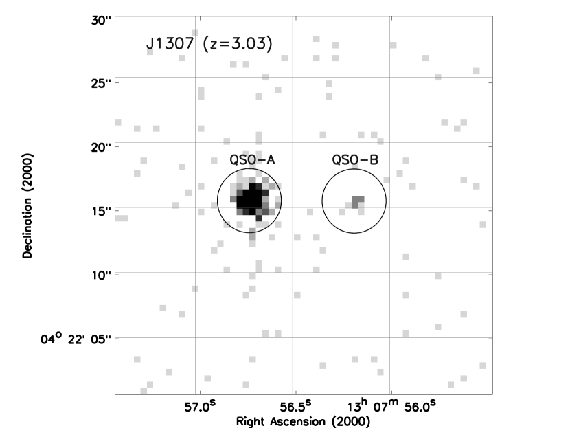
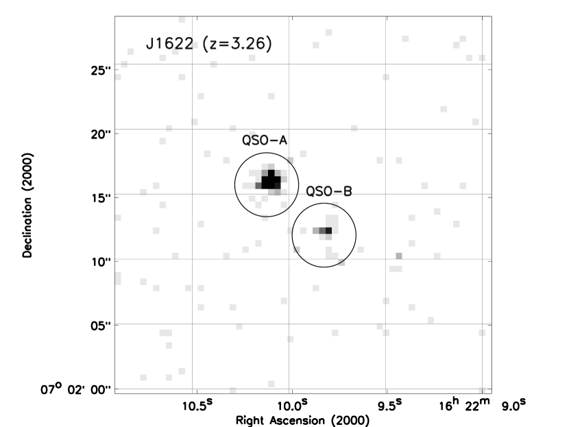
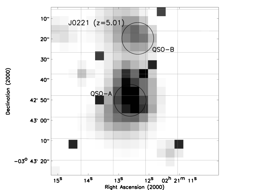
Figure 1: 0.5–7 keV band Chandra images of J1307 (top) and J1622 (middle) quasar fields. Each box side is 30^′′; the circles (diameter=5^′′) mark the quasars of the pairs. The QSO field of J0221 as observed by XMM-Newton (pn camera, 0.3–3 keV band) is shown in the bottom panel; each side of the box is $\approx$85^′′, and circles have a diameter of 15^′′. All images keep the original pixel size ($\approx$0.5^′′ for Chandra and $\approx 4.1$^′′ for XMM-Newton/pn).

3.1 Chandra data reduction

J1307 and J1622 were observed by Chandra in Cycle 15 on April 28^th and June 1^st, 2014, with the ACIS-S3 CCD at the aimpoint, for an effective exposure time of 64.22 ks and 65.06 ks, respectively. Source spectra were extracted using the CIAO software (v. 4.8) in the 0.5–7 keV band using a circular region with an extraction radius of 3.5^′′ and 1.7^′′ (J1307 A and B), and 2.5^′′ for both J1622 quasars. In all cases the background spectra were extracted from larger regions close to the source, avoiding the contribution from other sources. The number of source net counts are 845 (J1307A), 13 (J1307B), 215 (J1622A) and 30 (J1622B); spectra were therefore rebinned to 15 and 10 counts per bin for the two quasars with most counts, in order to apply the $\chi^{2}$ statistics, and to one count per bin for the sources with limited counting statistics; for these objects, the Cash statistics was used (Cash, 1979). All the spectral analyses were carried out using the xspec package (v.12.8; Arnaud 1996). Chandra cutouts in the 0.5–7 keV band are shown in the top (J1307) and middle (J1622) panels of Fig. 1.

3.2 XMM-Newton data reduction

J0221 was observed by XMM-Newton three times, twice within the XMM-LSS project (PI: M. Pierre) with nominal exposures of $\approx 14-15$ ks, and once to observe the low-mass cluster XLSSC 006 (PI: F. Pacaud) for a nominal exposure of $\approx 102$ ks. In the following we report the analysis of the data having the longest exposure. The data were reprocessed using the SAS software (v.15); high flaring background periods were removed with a sigma-clipping method, leaving a final exposure time of 68.3, 87.0 and 88.0 ks for the pn, MOS1 and MOS2 cameras, respectively. Source spectra for both quasar components were extracted from a circular region centered on their optical position; we used a radius of 15^′′ (corresponding to about 70 per cent of the pn encircled energy fraction at the source position) to maximise the source SNR and to prevent significant contamination by the relatively bright A component towards the much fainter B component; background spectra were extracted from a 30^′′ circular region in the same CCD as the source. We also checked that the apparently extended X-ray emission around J0221A (see the bottom panel of Fig. 1) was due to the relatively broad pn Point Spread Function (PSF); for this check, we used the SAS routine eradial, which allows a comparison between the source count distribution and the nominal PSF at a given position, fitted to the actual radial profile data. At the end of the spectral extraction procedure, the number of source net counts in the 0.5–7 keV band is 180 (pn) and 90 (MOS1$+$2) for the A component of the pair, and 50 for the fainter B component (only pn data were extracted). MOS1 and MOS2 spectra for J0221A were summed and, similarly to pn data, were grouped to have at least 10 counts per bin to apply the $\chi^{2}$ statistics; for the much fainter B component, Cash statistics was adopted in fitting the spectrum; a binning of one count per bin was applied in this case. The pn 0.3–3 keV image (maximising the emission of the faint B component) of J0221 is shown in the bottom panel of Fig. 1.

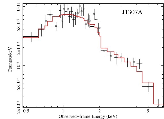
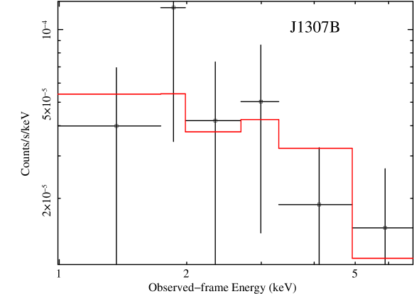
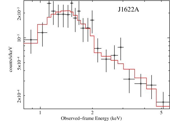
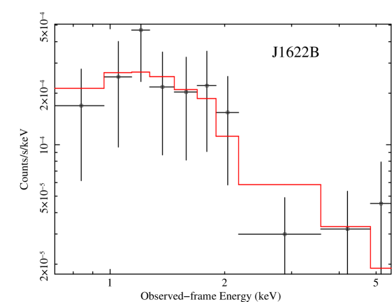
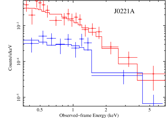
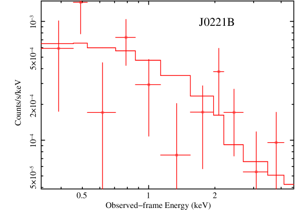
Figure 2: Chandra (top two rows) and XMM-Newton (bottom row) spectra of the three quasar pairs with best-fitting spectrum (continuous curve). The strong rebinning is for presentation purposes. For J0221A, both pn (red) and combined MOS1+2 (blue) spectra are shown; for J0221B, only the pn spectrum was extracted.

Table 2: X-ray spectral parameters of the quasar pairs derived from Chandra and XMM-Newton analysis.

Src.	$\Gamma$	NH	F${}_{2-10~{}keV}$	L${}_{2-10~{}keV}$	$\chi^{2}$(C-stat)/d.o.f.
		(cm-2)	(${\rm erg~{}cm}^{-2}~{}{\rm s}^{-1}$)	(erg s-1)
J1307A	1.53$\pm{0.10}$				44.3/48
	1.8$\dagger$	1.88${}^{+1.28}_{-1.02}\times 10^{22}$	8.6$\times 10^{-14}$	5.2$\times 10^{45}$	52.0/48
J1307B	0.4$\pm{1.0}$				9.7/10
	1.8$\dagger$	7.2${}^{+6.1}_{-4.7}\times 10^{23}$	4.0$\times 10^{-15}$	3.0$\times 10^{44}$	8.3/10
J1622A	1.21$\pm{0.20}$				15.5/19
	1.86${}^{+0.48}_{-0.44}$	1.77${}^{+1.42}_{-1.13}\times 10^{23}$	3.4$\times 10^{-14}$	2.6$\times 10^{45}$	8.2/18
J1622B	1.5$\pm{0.6}$		4.5$\times 10^{-15}$	1.9$\times 10^{44}$	10.7/27
	1.8$\dagger$	$<2.1\times 10^{23}$			10.6/27
J0221A	$2.14^{+0.26}_{-0.24}$		6.0$\times 10^{-15}$	1.9$\times 10^{45}$	34.6/38
	$2.22^{+0.50}_{-0.28}$	$<4.5\times 10^{22}$			34.5/37
J0221B	$1.6^{+0.6}_{-0.5}$		5.3$\times 10^{-15}$	6.9$\times 10^{44}$	91/114
	1.8$\dagger$	$<4.7\times 10^{22}$			85.3/114

Notes — $\dagger$ Fixed photon index. Fluxes are reported in the observed 2–10 keV band, while luminosities are intrinsic (i.e., corrected for obscuration, if present) and in the rest-frame 2–10 keV band. They are reported for the spectral fits which are considered to provide the best-fit description of the source emission. The last column indicates the quality of the fit in terms of either $\chi^{2}$ (A components) or C-stat (B components) over the number of degrees of freedom, depending on the statistics adopted in the spectral fitting (see text for details).

3.3 X-ray spectral analysis

Given the limited X-ray photon statistics available for the quasars under investigation, we adopted simple models, namely a power law and an absorbed power law. No additional component (e.g., reflection) seems to be present. All of the models take into account the Galactic absorption (Kalberla et al. 2005, see Table 1). In the following, errors and upper limits are reported at the 90 per cent confidence level for one parameter of interest (Avni, 1976), unless stated otherwise. Upper limits to the equivalent width (EW) of the iron K$\alpha$ emission line at 6.4 keV are reported in the source rest frame. Errors on the X-ray fluxes and luminosities are of the order of 6–30 per cent for the quasars with most counts, and 50–70 per cent for the quasars with poorer statistics.

J1307A. A power law well reproduces the emission for the A component ($\chi^{2}$/dof, degrees of freedom = 44.3/48); a photon index of $\Gamma=1.53\pm{0.10}$ is obtained. If we ascribe the apparently flat photon index (wrt. $\Gamma\approx 1.8-2.0$ typically observed in unobscured quasars; Piconcelli et al. 2005) to the presence of obscuration (i.e., fixing $\Gamma=1.8$ and leaving the column density free to vary), we derive $N_{\rm H}$=1.88${}^{+1.28}_{-1.02}\times 10^{22}$ cm^-2, i.e., moderate obscuration is possibly present in J1307A ($\chi^{2}$/dof=52.0/48). No iron emission line is required, the limit to the EW of the 6.4 keV component is 140 eV. The 2–10 keV flux is $\approx 8.6\times 10^{-14}$ ${\rm erg~{}cm}^{-2}~{}{\rm s}^{-1}$, corresponding to an intrinsic (i.e., corrected for the obscuration) rest-frame 2–10 keV luminosity of $\approx 5.2\times 10^{45}$ erg s^-1. The best-fitting spectrum is shown in Fig. 2 (top-left panel).

This source is the only quasar of the original H10 sample with a detection in the FIRST survey at 1.4 GHz (Becker, White, & Helfand, 1995); the flux density is $\approx$14.3 mJy. Using the available SDSS photometry and the definition of radio loudness as reported by Kellermann et al. (1989), $R$=$f_{\rm 5~{}GHz}/f_{\rm 4400~{}\mbox{\scriptsize\AA}}$ (rest frame), we are able to define J1307A as moderately radio loud (R$\approx$30). We checked for the presence of X-ray extension in this object, possibly related to some jet emission, by comparing the source count distribution vs. the PSF; we found no clear evidence for extension. However, the relatively flat photon index observed in this quasar ($\Gamma\approx 1.5$) may be due to the presence of an unresolved jet and associated X-ray emission (see Miller et al. 2011).

J1307B. This source is characterized by a C iv 1549Å BAL feature in the SDSS spectrum, indicative of extinction in an outflowing wind. BALQSOs are often characterized by obscuration also in the X-ray band (e.g., Green & Mathur 1996; Green et al. 2001; Shemmer et al. 2005; Giustini, Cappi, & Vignali 2008; see also Luo et al. 2013 for a different scenario). This is likely the most viable explanation for J1307B, whose spectrum is parametrized by a flat photon index ($\Gamma=0.4\pm{1.0}$). The flat X-ray slope supports the presence of obscuration; if this component is included in the spectral fitting and $\Gamma=1.8$ (fixed) is adopted, we obtain $N_{\rm H}$=7.2${}^{+6.1}_{-4.7}\times 10^{23}$ cm^-2 and a good fit (C-stat/dof=8.3/10); the spectrum is shown in Fig. 2, top-right panel. The source 2–10 keV flux and intrinsic rest-frame 2–10 keV luminosity are $\approx 4.0\times 10^{-15}$ ${\rm erg~{}cm}^{-2}~{}{\rm s}^{-1}$and $\approx 3.0\times 10^{44}$ erg s^-1, respectively. The upper limit to the neutral iron K$\alpha$ EW is $\approx$2 keV.

J1622A. Fitting the spectrum of J1622A with a power law results in $\Gamma=1.21\pm{0.20}$ ($\chi^{2}$/dof=15.5/19); the addition of absorption provides an improvement in the fitting ($\chi^{2}$/dof=8.2/18), and a more typical photon index of $\Gamma=1.86^{+0.48}_{-0.44}$ is derived. The column density is $N_{\rm H}$=1.77${}^{+1.42}_{-1.13}\times 10^{23}$ cm^-2. As for J1307B, J1622A can be optically classified as a BALQSO and is heavily obscured in X-rays. No iron line is detected (EW<300 eV). The source 2–10 keV flux (luminosity, corrected for the obscuration) is $\approx 3.4\times 10^{-14}$ ${\rm erg~{}cm}^{-2}~{}{\rm s}^{-1}$ ($\approx 2.6\times 10^{45}$ erg s^-1). The best-fitting spectrum is shown in Fig. 2 (middle-left panel).

J1622B. A power law with $\Gamma=1.5\pm{0.6}$ reproduces the X-ray emission of J1622B reasonably well (C-stat/dof=10.7/27). The inclusion of obscuration at the source redshift provides $N_{\rm H}$$<2.1\times 10^{23}$ cm^-2 (assuming $\Gamma$=1.8). No iron line is detected, the EW upper limit being $\approx$ 1.4 keV. The source 2–10 keV flux (luminosity) is $\approx 4.5\times 10^{-15}$ ${\rm erg~{}cm}^{-2}~{}{\rm s}^{-1}$ ($\approx 1.9\times 10^{44}$ erg s^-1). The best-fitting spectrum is shown in Fig. 2 (middle-right panel).

Summarizing, the analysis of the Chandra data indicates that the two quasars of the pairs which are classified as BALQSOs in the optical band are actually obscured in X-rays by column densities of the order of a few$\times 10^{23}$ cm^-2. All quasar luminosities are above 10⁴⁴ erg s^-1, with the two optically brightest members of the two pairs (the A quasars) having $L_{2-10~{}keV}>10^{45}$ erg s^-1. No indication of further components (e.g., reflection, iron emission line) is apparently present in the spectra. All of the spectral results are reported in Table 2.

J0221A. The pn and MOS1+2 spectra of J0221A were fitted simultaneously, leaving the normalizations of the pn and combined MOS cameras free to vary to account for possible (though minor) inter-calibration issues. A power law model with $\Gamma=2.14^{+0.26}_{-0.24}$ is able to reproduce the X-ray spectra well ($\chi^{2}$/dof=34.6/38), with no indication of further spectral complexities. The inclusion of obscuration at the source redshift provides a column density upper limit of $\approx 4.5\times 10^{22}$ cm^-2; the upper limit to the 6.4 keV iron line is $\approx$730 eV. The derived 2–10 keV flux (luminosity) is $\approx 6\times 10^{-15}$ ${\rm erg~{}cm}^{-2}~{}{\rm s}^{-1}$ ($\approx 1.9\times 10^{45}$ erg s^-1), with uncertainties of the order of 40 per cent. The best-fitting spectrum is shown in Fig. 2 (bottom-left panel).

J0221B. The photon statistics for J0221B (pn data) allows a basic parameterization of its spectrum; a single power law provides a good fit the the data (C-stat=91/114) and returns $\Gamma=1.6^{+0.6}_{-0.5}$. The obscuration, if present, is below $\approx 4.7\times 10^{22}$ cm^-2 (with $\Gamma$=1.8); the upper limit to the line EW is $\approx$450 eV. The derived 2–10 keV flux and rest-frame luminosity are $\approx 5.3\times 10^{-15}$ ${\rm erg~{}cm}^{-2}~{}{\rm s}^{-1}$  and $\approx 6.9\times 10^{44}$ erg s^-1, respectively, with uncertainties of the order of 70 per cent. The best-fitting spectrum is shown in Fig. 2 (bottom-right panel).

Table 3: Source parameters derived from the analysis of the optical spectra.

Src.	FWHM	F1350Å	Log(MBH/M⊙)	Lbol	$\Delta$v	$\lambda_{\rm Edd}$	Notes	SNR
(1)	(2)	(3)	(4)	(5)	(6)	(7)	(8)	(9)
J1307A	$7900\pm{170}$	$65\pm{2}$	9.5–10.0	27.8	$-1800\pm{970}$	0.21–0.76	SDSS BOSS	8
J1307B	$5440\pm{225}$	$14.6\pm{0.8}$	9.0–9.3	6.3	$-2240\pm{1030}$	0.24–0.45	SDSS BOSS$\dagger$	13
J1622A	$4870\pm{40}$	$158\pm{3}$	9.6–9.8	81.4	$-1000$	0.99–1.65	Keck (H10)$\dagger$	40
J1622B	$4970\pm{480}$	$6.5\pm{1.5}$	8.7–9.1	3.3	$-1000$	0.20–0.52	SDSS BOSS	4
J0221A	$3050\pm{55}$	$13.1\pm{1.6}$	8.6–9.1	18.8	$-2150\pm{610}$	1.07–3.30	SDSS	5
J0221B	$3810\pm{350}$	$2.2\pm{0.3}$	8.8	3.2		0.40	MMT$\ddagger$	3

(1) Source name; (2) FWHM of the C iv line (km/s); (3) value of the source continuum at 1350Å (in units of $10^{-17}$ ${\rm erg~{}cm}^{-2}~{}{\rm s}^{-1}$Å^-1), derived from the fitting of the optical spectrum; (4) logarithm of black hole mass (range) derived as described in $\S$4; the upper boundary is usually obtained using Eq. (2) of Shen et al. (2011b), the C iv FWHM and the 1350Å continuum luminosity; (5) bolometric luminosity (in units of 10⁴⁶ erg s^-1) derived from the 1350Å luminosity and adopting a bolometric correction of 3.8, valid for luminous SDSS quasars (see Richards et al. 2006); (6) blueshift of the C iv line computed with respect to C ii (measured in km s^-1). Reported errors have been estimated from Monte Carlo trials of mock spectra; see $\S\ref{optical}$ for details about J1622 quasars; (7) Eddington ratio range (where the bolometric luminosity is kept constant, while the Eddington luminosity takes into account the range of derived black hole masses); the Eddington ratio is defined as $\lambda_{\rm Edd}=L_{\rm bol}/L_{\rm Edd}$, where L_Edd is the Eddington luminosity ($\approx 1.3\times 10^{38}~{}(M_{\mathrm{BH}}/M_{\odot}$) erg s^-1); (8) origin of the optical spectrum used to derive the 1350Å continuum flux and the mass of the BH; (9) SNR of the optical continuum, close to the C iv line used to estimate the black hole mass. $\dagger$: classification as a BALQSO; $\ddagger$: provided by I. McGreer (McGreer et al., 2016).

4 Optical data analysis

Archival observed-frame optical spectra of the QSO pairs have been analysed to estimate SMBH properties (black hole masses, bolometric luminosities and accretion rates).

Four out of the six QSOs have been observed with different facilities (Keck, Magellan, MMT), while two have been observed two/three times as part of different SDSS programs. We used these spectra to check for the presence of spectral variability and the reliability of flux calibration. SDSS or SDSS-III Baryon Oscillation Spectroscopic Survey (BOSS; Dawson et al. 2013) spectra have been preferentially used to derive SMBH properties, because they typically have higher SNR (especially the BOSS ones). However, we analysed all available spectra to check the reliability of our results.

Before modelling the C iv line, for all sources but J0221B we subtracted the continuum emission fitting a power law at both sides of the ionized carbon line (in the two windows at 1330Å and 1690Å). The continuum in J0221B was instead modeled with a constant, given the low SNR. Then, we used a multi-Gaussian approach to best reproduce the total profile (see Fig. 3). We used up to three Gaussian profiles for the emission component. Negative narrow (broad) Gaussian lines with FWHM of few hundreds (thousands) of km/s have also been taken into account to reproduce narrow (broad) absorption line systems (NAL and BAL, respectively). Emission redwards of $\approx$1600Å can hardly be considered to be associated with C iv line (Fine et al., 2010) and was not taken into account in our analysis. Moreover, iron emission contamination (FeII and FeIII; Vestergaard & Wilkes 2001) in the region around C iv line is expected to be negligible (Shen et al., 2008, 2011b) and was not fitted.

Because of the complex shape of C iv emission (e.g., Gaskell 1982) and the issues regarding the presence and the treatment of C iv narrow line region emission in deriving black hole masses (see detailed discussion in Shen et al. 2011b; see also Dietrich et al. 2009 and Assef et al. 2011), we derived non-parametric widths following the prescriptions of Shen et al. (2011b), i.e. the FWHM of the best-fitting model profile. When NAL and BAL systems affect the C iv profile, we considered the total profile obtained from the only positive Gaussian components.

We derived black hole masses using the virial theorem and the broad-line region (BLR) radius – luminosity relation (Vestergaard & Peterson, 2006). The reliability of C iv virial mass estimator is, however, strongly debated. On the one hand, C iv scaling relation is still based on very few measurements (Kaspi et al., 2007; Saturni et al., 2016; Park et al., 2017). On the other hand, carbon line is often associated with blueshifted wings likely due to outflows (e.g. Richards et al. 2011); this non-virial component may affect the measurements of the total profile width and bias the black hole mass estimates. Empirical corrections have been proposed to reduce the bias (Denney, 2012; Park et al., 2013; Coatman et al., 2017) .

In Table 3 we report the range of values that can be derived using the relations by Shen et al. (2011b) (see their Eq. 2), Denney (2012) (Eq. 1), Park et al. (2013) (Eq. 3) and Coatman et al. (2017) (Eq. 6). The upper boundary value of each interval is usually obtained using the Shen et al. (2011b) prescriptions. The uncertainties in these measurements are dominated by the intrinsic scatter ($\approx 0.3$ dex, Park et al. 2017; Denney 2012; Vestergaard & Peterson 2006) in the single-epoch calibrations, which is much larger than the uncertainties ascribed to the quality of the analysed spectra ($\approx 0.01-0.05$ dex for the highest SNR spectra). To derive BH mass from Coatman et al. (2017) formula, we measured C iv offsets using systemic redshift when the low-ionization narrow line C ii is present in the spectra (see Table 3). For J1622A and J1622B, instead, we maximised the correction taking advantage of the anti-correlation between C iv velocity offset and EW (e.g., Coatman et al. 2017): starting from the SDSS DR7 QSO catalog of Shen et al. (2011b), for each of our targets we selected an SDSS subsample with similar C iv EW (within the errors). Then, we used these sources to construct a C iv velocity offset distribution and, from this, we derived the third quartile value. These velocities have been used to maximise the Coatman et al. (2017) BH mass correction of J1622A and J1622B.

Bolometric luminosity have been derived from the 1350Å luminosity, extrapolating the continuum power law to short wavelengths. We adopted a bolometric correction of 3.8, valid for luminous SDSS quasars and characterized by very limited scatter (see Richards et al. 2006). For J0221B, C iv line is at the edge of the spectral range covered by MMT, where the transmission is very low. In this case, the continuum luminosity has been derived through a modelling with a constant. The main quasar parameters from the analysis of the optical data are reported in Table 3.

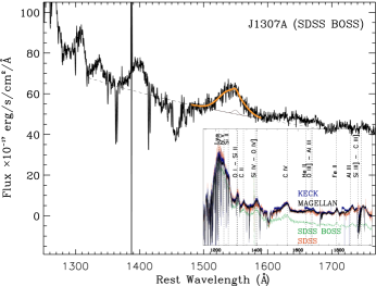
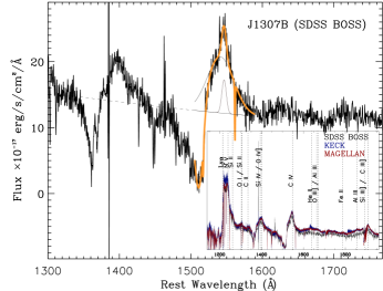
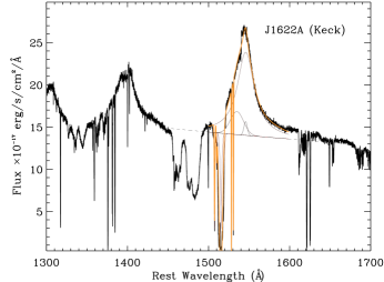
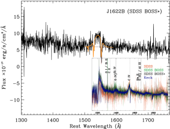
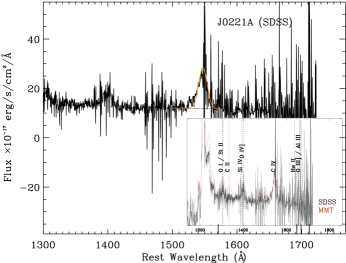
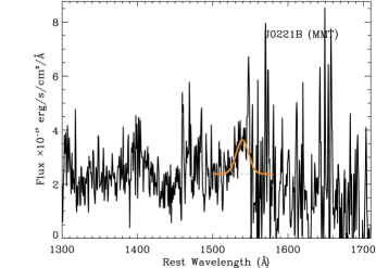
Figure 3: Rest-frame UV spectra of the quasar pairs around the C iv line showing our fitting method. Superimposed on the spectra are the best-fitting components (see $\S$ 4): a power law (dashed line), tracing the continuum emission, and Gaussian profiles (black solid curves), reproducing the C iv emission line. The orange solid curve represents the sum of all components, including a set of negative Gaussian profiles which take into account the BAL contribution when needed. In the insets, we show the various spectra of each quasar (when available) collected from archival data, which allowed us to prove the absence of significant luminosity variability, with the exception of J1307A. For J1307A and J1622B, we selected the SDSS BOSS spectra closer to the X-ray observation. For J0221B, the region at wavelength of 1545Å has been excluded from the fit, because of the strong sky-subtraction residuals affecting the C iv line profile (see Fig. 3 of McGreer et al. 2016). Vertical dotted lines mark the wavelength of UV emission lines in the range $1150-1950$Å.

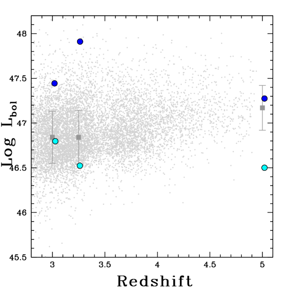
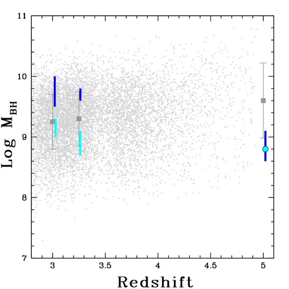
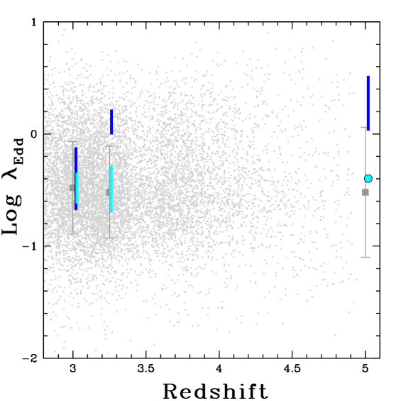
Figure 4: Comparison of the properties of the three quasar pairs of the current work vs. SDSS quasars (from the compilation of Shen et al. 2011b, updated as Nov. 2013, small grey dots): bolometric luminosity vs. redshift (left panel), black hole mass vs. redshift (middle panel) and Eddington ratio vs. redshift (right panel). The grey squares represent the median values from the SDSS quasars in redshift ranges encompassing/close to those of our sources, while the error bars show the 1-$\sigma$ dispersion. The A (B) quasar components of our sample are shown as blue (cyan) symbols and bars; the black hole mass and Eddington ranges (excluding J0221B) are computed as described in $\S$4, assuming negligible error on the derived bolometric luminosity (see Richards et al. 2011).

5 Properties of the quasar pairs at high redshift versus those of SDSS quasars

Although the sample of quasar pairs at high redshift presented in this work is limited, we made an attempt to verify whether, to first order, their properties strongly differ from those of luminous isolated quasars in the same redshift ranges. The results should give an idea on whether AGN in pairs have peculiar properties, maybe ascribed to the presence of the active companion on scales of several tens of kpc.

In primis, we have computed the source optical-to-X-ray power-law slope, $\alpha_{\rm ox}$, which is a measure of the relative importance of the emission disc vs. hot corona. It is defined as $\alpha_{\rm ox}=\frac{\log(f_{\rm 2~{}keV}/f_{2500~{}\mbox{\rm\scriptsize\AA}})}{\log(\nu_{\rm 2~{}keV}/\nu_{2500~{}\mbox{\rm\scriptsize\AA}})}$, where $f_{\rm 2~{}keV}$ and $f_{2500~{}\mbox{\scriptsize\rm\AA}}$ are the rest-frame flux densities at 2 keV and 2500 Å, respectively. These quantities have been obtained from the available X-ray spectra and optical photometry using the method outlined in Vignali, Brandt, & Schneider (2003). The 1-$\sigma$ errors on $\alpha_{\rm ox}$ are typically of $\approx 0.05-0.15$ once the uncertainties on the X-ray and optical values are considered (with the former contributing most). The $\alpha_{\rm ox}$ values of our non-BALQSOs ($\approx-1.4/-1.8$) are within the range expected for quasars once the $\alpha_{\rm ox}$ vs. 2500 Å luminosity anti-correlation (and relative scatter) is taken into account (e.g, Vignali, Brandt, & Schneider 2003; Shemmer et al. 2006; Just et al. 2007; Lusso et al. 2010; Nanni et al. 2017; Martocchia et al. 2017). The sources deviating most from the expected values, assuming the Just et al. (2007) relation, are those which are classified as BALQSOs in the present sample ($\approx-2.0/-2.2$). This is not unexpected, since steeper $\alpha_{\rm ox}$ (i.e., fainter soft X-ray emission at a given optical luminosity) are typically observed in absorbed sources as BALQSOs (e.g., Gibson et al. 2009).

For a more exhaustive comparison of our sample vs. high-redshift quasars, we have drawn three subsamples from the compilation of SDSS quasars published by Shen et al. (2011b), after checking that none of them has an active companion up to $\approx$100 kpc; in particular, we used the updated values of bolometric luminosities, black hole masses and Eddington ratios from the most recent (as Nov. 2013) version of the Shen catalog. For the J1307 quasar pair, we selected 1047 quasars at $z=2.95-3.05$, while for the J1622 system, 965 quasars were extracted at $z=3.20-3.30$. More challenging is to find an SDSS parent sample at $z\approx 5$: to this goal, we used the values from Shen et al. (2011b) for 55 quasars at $z=4.8-4.95$ (no quasar is present at higher redshift). The bolometric luminosities, black hole masses and Eddington ratios of the three subsamples are shown as little grey points in Fig. 4 (left, middle, and right panels, respectively); the median values and the dispersions of the distributions are reported as large grey squares and corresponding error bars. The values derived in $\S$4 for the three quasar pairs of this work are shown as blue and cyan symbols and bars for the A and B components of each pair, respectively (where bars take into account the range of black hole masses, hence of Eddington ratios, as described in $\S$4).

Starting from the derived bolometric luminosities (left panel in Fig. 4), we note that the A components of the $z\approx 3-3.3$ quasar pairs are well outside (and above) the median values of SDSS quasars; about the B components, J1622B is on the lower end of the 1$\sigma$ distribution, while J0221B is well below. However, the sampling of $z\approx 5$ quasars in Shen et al. (2011b) compilation is, as already stated, particularly scarce. Our results still hold if we compare the two BALQSOs, J1307B and J1622A, with the BALQSOs in Shen et al. (2011b) (166 and 135 at $z\approx 3$ and $z\approx 3.3$, respectively).

For what concerns the black hole masses (plotted as bars to take into account the range reported in Table 3, except for J0221B, for which only the Shen prescription has been adopted), the A components of our $z\approx 3-3.3$ pairs lie in the upper envelope of the SDSS BH mass distribution (middle panel of Fig. 4), although within the dispersion. J1622A is still located “high" in the distribution if the comparison is done against the BALQSOs at $z\approx 3.3$. Among the B components, the only “outlier" (but see the note of caution above) is J0221B, having a black hole mass apparently lower than the median of the distribution at $z\approx 5$. If we assumed an uncertainty for its black hole mass similar to that of its A companion, J0221B would be most likely within the dispersion of the distribution.

All these results translate into the right panel of Fig. 4, where the Eddington ratio (which is essentially the ratio of the quantities plotted in the y-axes in the other two panels, with the bars showing the range of black hole masses, hence Eddington luminosities) is reported for the three quasar pairs vs. SDSS quasars. Both J1307 A and B quasars are within the distribution; J1622A is above the median value (because of its very extreme bolometric luminosity) and a similar result is found for J0221A (in virtue of its relatively low BH mass).

The $z\approx 3.2$ quasar luminosity function (QLF) presented by Masters et al. (2012) allows us to place our $z\approx 3-3.3$ quasar pairs in a broader context: all of them populate the bright end of the QLF (on the basis of their rest-frame 1450Å absolute magnitudes, M₁₄₅₀), with J1622A being on one extreme (M${}_{1450}=-28.6$), and the companion, J1622B, being close to the knee of the QLF (with M${}_{1450}=-25.4$).

As already said, the comparison of the properties of J0221 quasars with those of quasars at similar redshift is more challenging. To understand how (a)typical J0221 quasars’ properties are (besides the uniqueness of this quasar pair at such high redshift; see the extended discussion in $\S 4.2$ of McGreer et al. 2016), we start computing their M₁₄₅₀ from the photometry reported in McGreer et al. (2016), obtaining M${}_{1450}\approx-26.9$ and M${}_{1450}\approx-25.0$ for J0221A and J0221B, respectively. Using, as reference, the work by McGreer et al. (2013), where the $z\approx 5$ QLF is derived by measuring the bright end with the SDSS and the faint end with the two-magnitude deeper SDSS data in the Stripe 82 region, J0221A clearly lies among the optically most luminous quasars and J0221B is around the mean. If we focus at $z=4.9-5.1$, J0221A is actually brighter by $\approx 0.3$ magnitude than the most luminous SDSS quasar reported in McGreer et al. (2013) in this redshift range, while J0221B is around the median value.

As previously stated, the main limitation of the current work lies on the small number of quasar pairs at high redshift with well defined multi-wavelength properties, including sensitive X-ray coverage to establish the level of nuclear activity. Extending the present sample would be important for a more solid assessment of the issues related on how the accretion-related activity in pairs is above the median value found for quasars not in pairs at similar redshifts. Such an extension, which could start from e.g. the compilation of H10, would be quite expensive in terms of observing time even with the present-day sensitive X-ray facilities (Chandra, XMM-Newton), as shown in the current work, where a good/moderately good description of quasar X-ray properties (continuum slope, column density, intrinsic luminosity) has required $\approx$ 65–80 ks exposures. We also note that in Cycle 15 the effective area of Chandra, especially in the soft band, was much higher than the current one (by about 60 per cent in the 0.5–7 keV band). Having said that, it seems that the presence of an active companion does not provide a substantial increase in terms of accretion (namely, Eddington ratio), and this appears to be consistent with the lack of signs of interactions in the available optical images of our target fields. The possible exception is represented by J1622A at $z\approx 3.3$ (and, more tentatively because of the limited comparison sample, of J0221A at $z\approx 5$). Focusing on J1622A, we computed the probability of extracting a bolometric luminosity higher than that of J1622A (8.14$\times 10^{47}$ erg s^-1; see Table 3) by chance from the sample of 965 SDSS quasars at $z=3.20-3.30$ reported above. We note that in this “parent" sample only five objects have a bolometric luminosity above that of J1622A and, in the same redshift range, there are three quasar pairs (hence six objects) in the H10 original sample. Thus we randomly extracted (one million trials) six quasars from the 965 SDSS quasar sample and obtained a bolometric luminosity above 8.14$\times 10^{47}$ erg s^-1 in 3.1 per cent of the cases. Therefore, our result of an increase of activity in J1622A due to the presence of an active companion has a not-negligible possibility to be obtained by chance (i.e., our result is significant at the $\approx 2.3\sigma$ level).

6 Summary of the results and conclusions

In this paper we have presented, for the first time, the X-ray and optical properties of three quasar pairs at $z\approx 3$ and $z\approx 3.3$ (selected from the SDSS and H10 work; their projected separations are 65 and 43 kpc, respectively) and $z\approx 5$ (selected from the CFHTLS, with a separation of 136 kpc; McGreer et al. 2016). The goal of this work, which benefits from the sensitivity and spatial resolution of Chandra (two 65-ks proprietary observations for the $z\approx 3-3.3$ systems) and XMM-Newton (one “cleaned" $\approx$80-ks archival pointing for the $z\approx 5$ system), is to provide some, though preliminary, indications on how accretion onto SMBHs and subsequent emission of radiation is possibly enhanced by the presence of an active companion on tens of kpc scales with respect to isolated quasars at similar redshifts. This is a first attempt, conducted on an admittedly small sample, to tackle the issues related to dual quasar activity at high redshift, whereas most of the studies carried out in recent years, at much lower redshifts ($z\lower 2.15277pt\hbox{$\;\buildrel<\over{\sim}\;$}0.2$) and luminosities, indicate enhanced BH and star-formation activity at close (several kpc) separations (e.g., Ellison et al. 2011). In the following we summarize the main results:
$\bullet$ Both quasar components of the three pairs are detected with relatively good photon statistics to allow us to derive the column density and intrinsic X-ray luminosity ($\approx$ a few 10${}^{44}-10^{45}$ erg s^-1  for all quasar pairs).
$\bullet$ Absorption of the order of a few $\times 10^{23}$ cm^-2 has been clearly detected in the two quasars of the systems at $z\approx 3.0-3.3$ (J1307B and J1622A) whose optical spectra are characterized by the presence of broad absorption features (likely associated with outflowing winds). This is not unexpected based on works on isolated BALQSOs at high redshift. Furthermore, tentative absorption of a few $\times 10^{22}$ cm^-2 has been found in J1307A, possibly suggesting that gas was destabilized in the central region of this object by the encounter with the companion.
$\bullet$ Using the information obtained from the analysis of the optical spectra of all quasar pairs, we derived bolometric luminosities, black hole masses and Eddington ratios. In particular, comparing their Eddington ratios vs. those of luminous SDSS quasars in the same redshift intervals we find that only one source, J1622A, lies significantly above the distribution of SDSS quasars at $z\approx 3.3$. One possible explanation of this result is that the high level of activity of J1622A (a bolometric luminosity of $\approx 8.1\times 10^{47}$ erg s^-1 for a $\log\ (M_{\rm BH}$/M_⊙)=9.6–9.8, about an order of magnitude higher than the bolometric luminosity of SDSS quasars at the same redshift) may be linked to the presence of the companion quasar. A statistical analysis of this result indicates a 3.1 per cent possibility that it is obtained by chance.

The results obtained for our sample of high-redshift dual quasars rely upon the limited number of quasars analysed thus far and the limited quality of X-ray spectra for some of them. To draw more solid conclusions in terms of properties of dual quasars at high redshifts and how these differ from those of quasars not in pairs at similar redshift, one would need deeper investigation with Chandra and XMM-Newton starting from the entire sample of H10, in which further six quasar pairs at separations $<100$ kpc are available (25 up to 650 kpc); another possibility, more suitable for Chandra given the low separations ($<6.3$^′′), consists in observing the sample presented by Eftekharzadeh et al. (2017). This project plan would match the large-project requirements for Chandra and XMM-Newton calls and, coupled with deep optical/near-IR observations, would allow also a study of source overdensities in these quasar fields.

A similar investigation, aimed at finding companions in our quasar fields, can be carried out in the submillimer by ALMA and NOEMA, using the molecular high-J CO transitions and the [C ii] lines as tracers of molecular and ionized gas and, possibly, the spectral scanning mode. With respect to other wavelengths (including X-rays, at least in part), submillimeter/far-infrared observations have the advantage of allowing potential detection, at high redshift, of very obscured AGN, besides galaxy companions (e.g., Carniani et al. 2013; Decarli et al. 2017). While galaxies at $z\approx 3.3$ can be found using the CO(4-3) transition (Band 3), systems at $z\approx 3.0$ and $z\approx 5.0$ in our quasar fields can be detected using the CO(5-4) line (Band 4 and 3, respectively). A similar search for companions would also benefit from the [C ii] line – particularly strong in star-forming systems – with observations in Band 8 and Band 7 for $z\approx 3-3.3$ and $z=5.0$ systems, respectively.

References

- Arnaud (1996) Arnaud K. A., 1996, ASPC, 101, 17
- Assef et al. (2011) Assef R. J., et al., 2011, ApJ, 742, 93
- Avni (1976) Avni Y., 1976, ApJ, 210, 642
- Ballo et al. (2004) Ballo L., Braito V., Della Ceca R., Maraschi L., Tavecchio F., Dadina M., 2004, ApJ, 600, 634
- Becker, White, & Helfand (1995) Becker R. H., White R. L., Helfand D. J., 1995, ApJ, 450, 559
- Begelman, Blandford, & Rees (1980) Begelman M. C., Blandford R. D., Rees M. J., 1980, Nature, 287, 307
- Bianchi et al. (2008) Bianchi S., Chiaberge M., Piconcelli E., Guainazzi M., Matt G., 2008, MNRAS, 386, 105
- Bogdanović (2015) Bogdanović T., 2015, ASSP, 40, 103
- Carniani et al. (2013) Carniani S., et al., 2013, A&A, 559, A29
- Cash (1979) Cash W., 1979, ApJ, 228, 939
- Coatman et al. (2017) Coatman L., Hewett P. C., Banerji M., Richards G. T., Hennawi J. F., Prochaska J. X., 2017, MNRAS, 465, 2120
- Comerford et al. (2012) Comerford J. M., Gerke B. F., Stern D., Cooper M. C., Weiner B. J., Newman J. A., Madsen K., Barrows R. S., 2012, ApJ, 753, 42
- Comerford et al. (2015) Comerford J. M., Pooley D., Barrows R. S., Greene J. E., Zakamska N. L., Madejski G. M., Cooper M. C., 2015, ApJ, 806, 219
- Conselice et al. (2003) Conselice C. J., Bershady M. A., Dickinson M., Papovich C., 2003, AJ, 126, 1183
- Dawson et al. (2013) Dawson K. S., et al., 2013, AJ, 145, 10
- Deane et al. (2014) Deane R. P., et al., 2014, Nature, 511, 57
- Decarli et al. (2017) Decarli R., et al., 2017, Natur, 545, 457
- Denney (2012) Denney K. D., 2012, ApJ, 759, 44
- Dietrich et al. (2009) Dietrich M., Mathur S., Grupe D., Komossa S., 2009, ApJ, 696, 1998
- Di Matteo, Springel, & Hernquist (2005) Di Matteo T., Springel V., Hernquist L., 2005, Nature, 433, 604
- Donley et al. (2018) Donley J. L., et al., 2018, ApJ, 853, 63
- Efstathiou & Rees (1988) Efstathiou G., Rees M. J., 1988, MNRAS, 230, 5
- Eftekharzadeh et al. (2017) Eftekharzadeh S., Myers A. D., Hennawi J. F., Djorgovski S. G., Richards G. T., Mahabal A. A., Graham M. J., 2017, MNRAS, 468, 77
- Ellison et al. (2011) Ellison S. L., Patton D. R., Mendel J. T., Scudder J. M., 2011, MNRAS, 418, 2043
- Ellison et al. (2013) Ellison S. L., Mendel J. T., Scudder J. M., Patton D. R., Palmer M. J. D., 2013, MNRAS, 430, 3128
- Escala et al. (2004) Escala A., Larson R. B., Coppi P. S., Mardones D., 2004, ApJ, 607, 765
- Fan et al. (2001) Fan X., et al., 2001, AJ, 122, 2833
- Fine et al. (2010) Fine S., Croom S. M., Bland-Hawthorn J., Pimbblet K. A., Ross N. P., Schneider D. P., Shanks T., 2010, MNRAS, 409, 591
- Fu et al. (2011) Fu H., et al., 2011, ApJ, 740, L44
- Gaskell (1982) Gaskell C. M., 1982, ApJ, 263, 79
- Gibson et al. (2009) Gibson R. R., et al., 2009, ApJ, 692, 758
- Giustini, Cappi, & Vignali (2008) Giustini M., Cappi M., Vignali C., 2008, A&A, 491, 425
- Green & Mathur (1996) Green P. J., Mathur S., 1996, ApJ, 462, 637
- Green et al. (2001) Green P. J., Aldcroft T. L., Mathur S., Wilkes B. J., Elvis M., 2001, ApJ, 558, 109
- Green et al. (2010) Green P. J., Myers A. D., Barkhouse W. A., Mulchaey J. S., Bennert V. N., Cox T. J., Aldcroft T. L., 2010, ApJ, 710, 1578
- Green et al. (2011) Green P. J., Myers A. D., Barkhouse W. A., Aldcroft T. L., Trichas M., Richards G. T., Ruiz Á., Hopkins P. F., 2011, ApJ, 743, 81
- Guainazzi et al. (2005) Guainazzi M., Piconcelli E., Jiménez-Bailón E., Matt G., 2005, A&A, 429, L9
- Haehnelt & Kauffmann (2002) Haehnelt M. G., Kauffmann G., 2002, MNRAS, 336, L61
- Hennawi et al. (2010) Hennawi J. F., et al., 2010, ApJ, 719, 1672 (H10)
- Hopkins et al. (2008) Hopkins P. F., Hernquist L., Cox T. J., Kereš D., 2008, ApJS, 175, 356
- Jiang et al. (2016) Jiang L., et al., 2016, ApJ, 833, 222
- Jiménez-Bailón et al. (2007) Jiménez-Bailón E., Loiseau N., Guainazzi M., Matt G., Rosa-González D., Piconcelli E., Santos-Lleó M., 2007, A&A, 469, 881
- Just et al. (2007) Just D. W., Brandt W. N., Shemmer O., Steffen A. T., Schneider D. P., Chartas G., Garmire G. P., 2007, ApJ, 665, 1004
- Kalberla et al. (2005) Kalberla P. M. W., Burton W. B., Hartmann D., Arnal E. M., Bajaja E., Morras R., Pöppel W. G. L., 2005, A&A, 440, 775
- Kaspi et al. (2007) Kaspi S., Brandt W. N., Maoz D., Netzer H., Schneider D. P., Shemmer O., 2007, ApJ, 659, 997
- Kellermann et al. (1989) Kellermann K. I., Sramek R., Schmidt M., Shaffer D. B., Green R., 1989, AJ, 98, 1195
- Komossa et al. (2003) Komossa S., Burwitz V., Hasinger G., Predehl P., Kaastra J. S., Ikebe Y., 2003, ApJ, 582, L15
- Komossa & Zensus (2016) Komossa S., Zensus J. A., 2016, IAUS, 312, 13
- Koss et al. (2012) Koss M., Mushotzky R., Treister E., Veilleux S., Vasudevan R., Trippe M., 2012, ApJ, 746, L22
- Imanishi & Saito (2014) Imanishi M., Saito Y., 2014, ApJ, 780, 106
- Lin et al. (2008) Lin L., et al., 2008, ApJ, 681, 232-243
- Liu et al. (2011) Liu X., Shen Y., Strauss M. A., Hao L., 2011, ApJ, 737, 101
- Liu, Shen, & Strauss (2012) Liu X., Shen Y., Strauss M. A., 2012, ApJ, 745, 94
- López-Sanjuan et al. (2013) López-Sanjuan C., et al., 2013, A&A, 553, A78
- Luo et al. (2013) Luo B., et al., 2013, ApJ, 772, 153
- Lusso et al. (2010) Lusso E., et al., 2010, A&A, 512, A34
- Martocchia et al. (2017) Martocchia S., et al., 2017, A&A, 608, A51
- Masters et al. (2012) Masters D., et al., 2012, ApJ, 755, 169
- McGreer et al. (2013) McGreer I. D., et al., 2013, ApJ, 768, 105
- McGreer et al. (2016) McGreer I. D., Eftekharzadeh S., Myers A. D., Fan X., 2016, AJ, 151, 61
- Miller et al. (2011) Miller B. P., Brandt W. N., Schneider D. P., Gibson R. R., Steffen A. T., Wu J., 2011, ApJ, 726, 20
- Mortlock, Webster, & Francis (1999) Mortlock D. J., Webster R. L., Francis P. J., 1999, MNRAS, 309, 836
- Mudd et al. (2014) Mudd D., et al., 2014, ApJ, 787, 40
- Nanni et al. (2017) Nanni R., Vignali C., Gilli R., Moretti A., Brandt W. N., 2017, A&A, 603, A128
- Onoue et al. (2018) Onoue M., et al., 2018, PASJ, 70, S31
- Park et al. (2013) Park D., Woo J.-H., Denney K. D., Shin J., 2013, ApJ, 770, 87
- Park et al. (2017) Park D., Barth A. J., Woo J.-H., Malkan M. A., Treu T., Bennert V. N., Assef R. J., Pancoast A., 2017, ApJ, 839, 93
- Piconcelli et al. (2005) Piconcelli E., Jimenez-Bailón E., Guainazzi M., Schartel N., Rodríguez-Pascual P. M., Santos-Lleó M., 2005, A&A, 432, 15
- Piconcelli et al. (2010) Piconcelli E., et al., 2010, ApJ, 722, L147
- Ricci et al. (2017) Ricci C., et al., 2017, MNRAS, 468, 1273
- Richards et al. (2006) Richards G. T., et al., 2006, ApJS, 166, 470
- Richards et al. (2011) Richards G. T., et al., 2011, AJ, 141, 167
- Saturni et al. (2016) Saturni F. G., Trevese D., Vagnetti F., Perna M., Dadina M., 2016, A&A, 587, A43
- Shangguan et al. (2016) Shangguan J., Liu X., Ho L. C., Shen Y., Peng C. Y., Greene J. E., Strauss M. A., 2016, ApJ, 823, 50
- Shemmer et al. (2005) Shemmer O., Brandt W. N., Gallagher S. C., Vignali C., Boller T., Chartas G., Comastri A., 2005, AJ, 130, 2522
- Shemmer et al. (2006) Shemmer O., et al., 2006, ApJ, 644, 86
- Shen et al. (2008) Shen Y., Greene J. E., Strauss M. A., Richards G. T., Schneider D. P., 2008, ApJ, 680, 169
- Shen et al. (2011a) Shen Y., Liu X., Greene J. E., Strauss M. A., 2011a, ApJ, 735, 48
- Shen et al. (2011b) Shen Y., et al., 2011b, ApJS, 194, 45
- Silk & Rees (1998) Silk J., Rees M. J., 1998, A&A, 331, L1
- Tasca et al. (2014) Tasca L. A. M., et al., 2014, A&A, 565, A10
- Vestergaard & Wilkes (2001) Vestergaard M., Wilkes B. J., 2001, ApJS, 134, 1
- Vestergaard & Peterson (2006) Vestergaard M., Peterson B. M., 2006, ApJ, 641, 689
- Vignali, Brandt, & Schneider (2003) Vignali C., Brandt W. N., Schneider D. P., 2003, AJ, 125, 433
- Volonteri, Haardt, & Madau (2003) Volonteri M., Haardt F., Madau P., 2003, ApJ, 582, 559
- Yuan, Strauss, & Zakamska (2016) Yuan S., Strauss M. A., Zakamska N. L., 2016, MNRAS, 462, 1603