A Particle Physics Origin of the 5 MeV Bump in the Reactor Antineutrino Spectrum?

Abstract

One of the most puzzling questions in neutrino physics is the origin of the excess at 5 MeV in the reactor antineutrino spectrum. In this paper, we explore the excess via the reaction ¹³C$(\overline{\nu},\overline{\nu}^{\prime}n)^{12}$C^∗ in organic scintillator detectors. The de-excitation of ¹²C^∗ yields a prompt $4.4$ MeV photon, while the thermalization of the product neutron causes proton recoils, which in turn yield an additional prompt energy contribution with finite width. Together, these effects can mimic an inverse beta decay event with around 5 MeV energy. We consider several non-standard neutrino interactions to produce such a process and find that the parameter space preferred by Daya Bay is disfavored by measurements of neutrino-induced deuteron disintegration and coherent elastic neutrino-nucleus scattering. While non-minimal particle physics scenarios may be viable, a nuclear physics solution to this anomaly appears more appealing.

I Introduction

Neutrinos from nuclear reactors have a prominent role in the field of neutrino physics; neutrinos were discovered using reactors as sources, and $\theta_{13}$ was shown to be nonzero using detectors close to a nuclear reactor [1, 2, 3]. Currently, reactor experiments are grappling with two anomalous findings. The first is the $\sim 6$% mismatch between the predicted and observed rates in short-baseline reactor experiments that could be explained via oscillations into additional, eV-scale neutrinos [4]. The other, more recent one is the excess of neutrino events around 5 MeV, the so-called reactor bump [5]. This spectral feature has triggered significant interest in the community in recent years [6, 7, 8], but has thus far eluded any quantitative explanation in terms of nuclear physics. Moreover, no attempts in terms of beyond the Standard Model (SM) physics can be found in the literature. Due to the lack of general agreement on the source of the discrepancy, it appears meaningful to explore potential for explaining the 5 MeV bump with new physics (NP).

Current reactor experiments detect neutrinos via inverse beta decay (IBD): $\bar{\nu}_{e}+p\rightarrow n+e^{+}$. The signature used to identify these events and separate them from background is the delayed coincidence between the positron, $e^{+}$ – which forms the prompt signal – and the neutron capture on gadolinium and the subsequent emission of a gamma cascade of about 8 MeV total energy – the delayed signal, some 50–100 $\mu$s later. The positron signal has no specific characteristics and any prompt energy deposition in the detector could be mistaken as the prompt signal. It is the delayed neutron capture signal which is essentially background free, i.e., only neutrons can cause it, which then allows to tag the prompt signal as being part of an IBD event. Under these conditions, it is clear that any new physics explanation must produce a neutron in its final state. It also has been established that the bump tracks reactor power and thus has to be caused by a particle flux from the reactor which is closely related to the number of beta decays inside the reactor. Beta decays of any known isotope extend at most to Q-values of 15–20 MeV, and thus, direct production of a neutron from any particle flux from a reactor is excluded. Therefore, a neutron which is already present in the detector material has to be liberated from its nuclear bound state.

Liquid scintillator as used in Daya Bay and NEOS is made up of carbon and hydrogen. Hydrogen has only about a 1:10,000 admixture of deuterium; thus, the only neutron source is carbon. Carbon-12 has a neutron separation energy of 18.7 MeV and thus there are no particles energetic enough coming from the reactor which can effect this reaction. On the other hand, carbon-13 has an abundance of about 1% and a neutron separation energy of only 4.9 MeV, well within the energies available in beta decay. The reaction ¹³C$(\bar{\nu},\bar{\nu}^{\prime}n)^{12}$C can proceed via the ground state of ¹²C or via the first excited state at 4.4 MeV, which then would de-excite immediately via the emission of a 4.4 MeV gamma, which naturally would appear as a line-like energy deposition close to the bump energy. Additional prompt energy will be supplied by the neutron kinetic energy: the neutron loses its energy by collisions with carbon and hydrogen and the recoiling nuclei will leave a scintillation signature. Due to the details of scintillation light emission, explained in more detail later, and the stochastic nature of neutron energy losses, this recoil signal will add the missing energy to match the mean bump energy as well as give the requisite width to the signal. Note, that this is a minimal scenario from a phenomenological view point and apart from the interaction causing the anomalously high ¹³C scattering rate, all ingredients are well-known Standard Model physics. In particular, the bump position and width are determined by known physics.

In this paper, we will first explore the details of signal formation and demonstrate that it actually provides an excellent description of the experimental data. Then we proceed, in the spirit of low-energy effective field theory, to explore possible operators that could cause the anomalously high ¹³C scattering rate and examine if other data rule out these operators at the required strength. We are looking for neutral-current-like operators of the form

$$2\sqrt{2}G_{f}\epsilon(\bar{\nu}_{s}L\nu_{s})(\bar{N}LN)\,,$$ (1)

where $N$ denotes a nucleon and $L$ is an arbitrary Lorentz structure, i.e., $L=1,\,\gamma_{5},\,\gamma^{\mu},\,\gamma^{\mu}\gamma_{5},\,\ldots$. The strength of the new interaction, $\epsilon$, is bounded from below by the fact that the bump is about 10% of the regular IBD signal. Combined with the 1% abundance of ¹³C, this implies that $\epsilon>10$. Invariance under SU(2)_EW implies the existence of a corresponding term involving charged leptons; any such operator with the required interaction strength will be ruled out by charged-lepton data. We circumvent this restriction by introducing an additional neutrino state that is not part of an electroweak multiplet. We can choose the new mixing angle and new mass splitting to be consistent with this additional neutrino being the explanation of the reactor antineutrino anomaly [4].

We argue that this constitutes a phenomenological minimal framework to seek a BSM explanation of the 5 MeV bump and we provide the quantitative demonstration that this framework indeed explains the reactor data. We also will demonstrate that any minimal incarnation of the operator in Eq. 1 is ruled out by either COHERENT [9] data or past reactor neutrino deuterium scattering results [10].

II Cross section and Neutrino fluxes

II.1 Obtaining the new physics cross section

A first-principles calculation of the ¹³C$(\bar{\nu},\bar{\nu}^{\prime}n)^{12}$C^(∗) cross section for a given NP model is beyond the scope of this work. Here, we illustrate our estimation of the cross section using measurements of ¹³C$(e,e^{\prime}n)^{12}$C^(∗) as a proxy for the NP ¹³C$(\bar{\nu},\bar{\nu}^{\prime}n)^{12}$C^(∗) cross section. In doing so, we are implicitly assuming the existence of a new vector interaction; we discuss this scenario in more detail in section IV. We assume that nuclear physics effects in the exchange of the hidden vector particle, dubbed $X$, are not qualitatively different from the SM photon case.

The differential cross section for ¹³C$(e,e^{\prime}n)^{12}$C^(∗) is parameterized in Ref. [11] by

$$\frac{d^{2}\sigma}{dE_{n}d\Omega}(E_{i},E_{n})=4\pi A_{0}(E_{n})\frac{d\sigma_{\rm Mott}}{d\Omega_{f}}\left(E_{i},E_{n}\right)\,,$$ (2)

where $E_{i}$ is the initial-state electron energy, $E_{n}$ is the neutron kinetic energy, $\Omega_{f}$ is the final-state electron solid angle, $A_{0}$ is an experimentally-determined function of the energy transferred to the nuclear system [11] and $d\sigma_{\text{Mott}}/d\Omega_{f}$ is the differential Mott cross section for an electron scattering off a heavy, point-like nucleus in QED.

The Mott cross section in eq. 2 is formally divergent; we regulate it by introducing a finite mass $M_{X}$ for $X$ and find

$$\frac{d\sigma_{\rm Mott}}{d\Omega_{f}}\left(E_{i},E_{n}\right)=\frac{2\alpha^{2}Z^{2}E_{i}E_{f}(1-\cos\theta_{f})}{\left(M_{X}^{2}+2E_{i}E_{f}(1-\cos\theta_{f})\right)^{2}},$$ (3)

where $E_{f}=E_{i}-E_{n}-E_{\rm th}$ is the final-state electron energy and $E_{\rm th}$ is the threshold energy for the reaction. For transitions to the ground state of ¹²C, $E_{\rm th}\approx$ 4.9 MeV, while for transitions to the first excited state, $E_{\rm th}\approx$ 9.3 MeV. Integrating eq. 3 over $d\Omega_{f}$ yields

$$\sigma_{\rm Mott}= \,\,\frac{\pi\alpha^{2}Z^{2}}{E_{i}E_{f}}\times$$ (4)

$$\left[\log\left(\frac{4E_{i}E_{f}+M_{X}^{2}}{M_{X}^{2}}\right)-\frac{4E_{i}E_{f}}{4E_{i}E_{f}+M_{X}^{2}}\right].$$

We convert the $(e,e^{\prime}n)$ cross section $\sigma$ into the NP cross section $\sigma^{\prime}$ for the $(\bar{\nu},\bar{\nu}^{\prime}n)$ reaction by rescaling the former by an effective coupling $\zeta^{2}$. The resulting neutron spectrum is

$$\frac{d\sigma^{\prime}}{dE_{n}}(E_{\overline{\nu}},E_{n})={\zeta^{2}}\times\frac{d\sigma}{dE_{n}}(E_{i}=E_{\overline{\nu}},E_{n})\,,$$ (5)

where $E_{\bar{\nu}}$ is the energy of an incoming neutrino and $d\sigma/dE_{n}=4\pi A_{0}\sigma_{\rm Mott}$. Convolving this neutron spectrum with the reactor antineutrino flux, $\phi_{\bar{\nu}}$, yields the cross-section-weighted neutron spectrum, $\widetilde{\phi}_{n}$,

$$\frac{d\widetilde{\phi}_{n}}{dE_{n}}(E_{n})=0.006\times\int dE_{\overline{\nu}}\,\frac{d\sigma^{\prime}}{dE_{n}}(E_{\overline{\nu}},E_{n})\cdot\frac{d\phi_{\bar{\nu}}}{dE_{\overline{\nu}}}(E_{\overline{\nu}}),$$ (6)

where “0.006” accounts for the difference in the number of protons and carbon atoms in the linear alkylbenzene (LAB), $\left(\text{C}_{6}\text{H}_{5}\right)\text{C}_{n}\text{H}_{2n+1}$ ($n\sim 10-16$), used by Daya Bay, as well as the natural abundance of ¹³C ($1.07\%$). Once detector effects are included, this spectrum is added to the IBD prompt-energy spectrum in order to replicate the 5 MeV bump.

II.2 Reactor Antineutrino fluxes

The ¹³C$(\bar{\nu},\bar{\nu}^{\prime}n)^{12}$C^∗ reaction requires a significant neutrino flux above $E_{\bar{\nu}}\gtrsim 9.4$ MeV, though reactor experiments have measured the flux only up to 8 MeV, e.g., see Ref. [12]. The Huber-Mueller (HM) fluxes [13, 14] do not extend beyond 9 MeV. On the other hand, ab initio calculations of reactor fluxes [15] predict a nonzero flux up to energies of 16 MeV. Preliminary upper bounds of the neutrino flux beyond 8 MeV have been reported by Daya Bay [16] and our fit does not exceed these bounds. We augment the HM fluxes by including an additional power-law component beyond 8 MeV, described by a power-law index $I$, such that the flux is continuous at $E_{\bar{\nu}}=8$ MeV.

A popular alternative explanation for the reactor bump is that the neutrino flux from ²³⁸U has been miscalculated; there exists mounting evidence supporting a connection between the strength of the reactor bump and the ²³⁸U fuel fraction of the reactor (see Refs. [17, 6] for more details). This explanation and that proposed here are not mutually exclusive; if the flux of high-energy antineutrinos from ²³⁸U has been underestimated, then this may provide the additional flux that we require to reproduce the bump.

II.3 Neutron thermalization

Neutrons lose energy via elastic collisions with the atoms in the scintillator; we simulate these stochastic energy losses with a simple Monte Carlo calculation. To determine the amount of prompt energy from the proton recoils, we account for quenching in the liquid scintillator, assuming nonrelativistic protons. The amount of energy produced by the scintillator is given by Birks’ law [18],

$$E=\int\frac{\left(\frac{dE}{dx}\right)dx}{1+k_{B}\left(\frac{dE}{dx}\right)},$$ (7)

where $k_{B}=0.0065$ g cm^-2 MeV^-1 is Birks’ constant for Gd-doped LAB [19] as used in Daya Bay. The quenching factor $Q=E(k_{B})/E(k_{B}\to 0)$ is calculated via eq. 7 using the proton $dE/dx$ in organic scintillator [20]. The combined effects of the stochastic proton energy distribution and quenching give rise to a finite width for the prompt energy reconstructed from this process.

III FIT

We simulate ¹³C–$\overline{\nu}$ events using Monte Carlo methods for the following ranges of $X$ masses, effective couplings and power-law indices to determine the prompt energy spectrum at Daya Bay detector(s):

$$M_{X} \in$$ [1 keV, 1 GeV]

$$\log_{10}\zeta \in [-12.3,\,1.7]$$

$$I \in [5,\,20]$$

The smeared spectrum is compared against the ratio of measurement-to-expectation of the prompt energy spectrum reported in Ref. [6] using a standard $\chi^{2}$-test, incorporating uncertainties on and correlations between the Daya Bay data, theoretical uncertainties in the HM fluxes and experimental uncertainties on $A_{0}(E_{n})$.

Figure 1: The prompt energy spectrum corresponding to the best-fit point in eq. 8. Only transitions to the first excited state of ¹²C have been included. See text for details.

Figure 2: The same as fig. 1, except that transitions to the ground state of ¹²C have been included. See text for details.

Considering only transitions to the excited state of ¹²C, the minimum value of the $\chi^{2}$, $\chi^{2}_{\rm min}$, is 10.3 and occurs for

$$\{M_{X},\,\log_{10}\zeta,\,I\}=\{1\text{ keV},\,-6.075,\,13\};$$ (8)

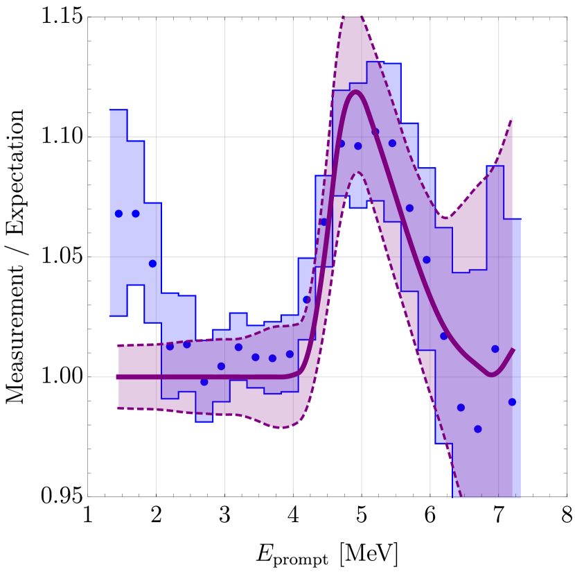
for 21 degrees of freedom (d.o.f.), this is equivalent to $p=0.97$. The curve corresponding to this best-fit point is shown in fig. 1. The blue circles and blue bands correspond to the Daya Bay data and their associated uncertainties; the solid, purple line is calculated for the parameters in eq. 8 and the dotted, purple lines show the uncertainties on the neutrino spectrum and the measurements of $A_{0}(E_{n})$, which have been added in quadrature. Marginalizing over the power-law index gives $\chi^{2}_{\rm min}$/d.o.f. = 9.1/22 ($p=0.99$), compared to $35.1/24$ ($p=0.07$) in the absence of any NP.

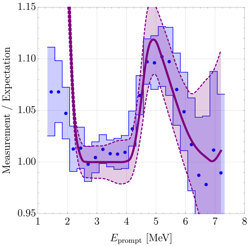
When transitions to the ground state of ¹²C are included, the best-fit prompt energy spectrum presents a steep upturn at low energies; the fit cannot reproduce the 5 MeV bump without overproducing low-energy events by a factor of $\sim 10$, as shown in fig. 2. For the best-fit point in eq. 8, including transitions to the ground state increases $\chi^{2}_{\rm min}$/d.o.f. to $49.1/21$ ($p=4.9\times 10^{-4}$). We estimate that a $\lesssim\mathcal{O}(10\%)$ suppression of these transitions is sufficient to avoid problems. For a purely vector interaction, such a suppression is entirely ad hoc. However, if the new interaction were axial in nature, then it is likely to significantly suppress (or eliminate altogether) such transitions: the ¹³C ground state has $J^{\pi}=1/2^{-}$, whereas the ¹²C ground state has $J^{\pi}=0^{+}$ and the first excited state in ¹²C has $J^{\pi}=2^{+}$. A full calculation using the ¹³C and ¹²C wave functions is beyond the scope of this work.

We have also explored the effects of a threshold $Q_{\text{th}}^{2}$ in the momentum exchange $-q^{2}=2E_{i}E_{f}(1-\cos\theta_{f})$ to determine if this can lead to the required suppression of the ground state transitions, which are generally characterized by smaller momentum exchanges. The effects of a threshold can be equivalently represented by an upper bound $\cos\theta_{f}<1-Q_{\rm th}^{2}/2E_{i}E_{f}$. The total Mott cross section becomes

$$\sigma_{\rm Mott}= \,\,\frac{\pi\alpha^{2}Z^{2}}{E_{i}E_{f}}\times\left[\log\left(\frac{4E_{i}E_{f}+M_{X}^{2}}{M_{X}^{2}+Q_{\rm th}^{2}}\right)\right.$$

$$\left.-\frac{M_{X}^{2}(4E_{i}E_{f}-Q_{\rm th}^{2})}{(4E_{i}E_{f}+M_{X}^{2})(M_{X}^{2}+Q_{\rm th}^{2})}\right];$$ (9)

in contrast with eq. 4, in which no threshold is present.

Scenario	$\chi^{2}_{\rm min}$	d.o.f.	$p$
No NP	35.1	24	0.07
NP, $Q_{\rm th}$ = 0 MeV	16.8	22	0.77
NP, $Q_{\rm th}$ = 5 MeV	17.3	22	0.75
NP, $Q_{\rm th}$ = 10 MeV	17.1	22	0.76
NP, $Q_{\rm th}$ = 15 MeV	16.8	22	0.77
NP, No Ground State	9.1	22	0.99

Table 1: The values of $\chi^{2}_{\rm min}$ for the cases in which NP is not present; where it is present, but there is no threshold $Q_{\rm th}$ in the momentum transfer; and in the cases where this threshold is 5, 10 or 15 MeV. We also show the number of degrees of freedom (“d.o.f.”) in each fit, as well as the corresponding $p$-value. Transitions to the ground state of ¹²C are unsuppressed in these analyses. In the last row, we show the value of the $\chi^{2}_{\rm min}$ for the case in which transitions to the ground state are totally suppressed, for comparison.

The results of this analysis are shown in Table 1. The fits are obtained in a similar fashion as described for the scenario with no threshold, except that transitions to the ground state of ¹²C are unsuppressed. It is clear that nonzero $Q_{\rm th}$ has not appreciably lowered $\chi^{2}_{\rm min}$ relative to the case in which $Q_{\rm th}=0$. Together with the increased challenge of constructing a model that would exhibit this kind of behavior (since stronger NP interactions would be required), this does not seem like a viable way to suppress ground-state transitions.

Taken at face value, including the ground-state transitions still seems to be a modest improvement over the SM prediction, even if ignoring them provides a better fit. However, most of the improvement to the fit in the former case comes from fitting the upturn at low energies in the Daya Bay data; the best-fit solution does little to reproduce the 5 MeV bump. We perform a similar analysis in which we omit the six lowest-energy Daya Bay data points to isolate the 5 MeV bump. With this restriction, the best-fit point is identical to that of eq. 8 (independent of our previous analysis), and $\chi^{2}_{\rm min}$/d.o.f., having marginalized over the power-law index, is 1.4/16 ($1-p=8.9\times 10^{-7}$). The equivalent result in the absence of NP is 24.1/18 ($p=0.09$). Importantly, this result is independent of whether or not ground-state transitions are included in the analysis. As such, the inclusion of ground-state transitions has no effect on the 5 MeV bump itself; they only cause the fit to struggle to reconcile the bump with the upturn in the low-energy data.

We briefly consider the NEOS experiment [21] which sees a similar bump at 5 MeV in their prompt energy spectrum. Including only transitions to the first excited state of ¹²C and marginalizing over the power-law index, we find $\chi^{2}_{\rm min}$/d.o.f. $=14.2/58$ ($1-p=6.2\times 10^{-10}$) at the best-fit point compared to $66.7/60$ ($p=0.26$) without NP. Moreover, the results of Daya Bay and NEOS are consistent with one another; analyzing both simultaneously gives $\chi^{2}_{\rm min}$/d.o.f. $=101.8/84$ ($p=0.09$) in the absence of NP, while $\chi^{2}_{\rm min}$/d.o.f. $=24.0/82$ ($1-p=4.7\times 10^{-11}$) is obtained with transitions only to the first excited state of ¹²C. We demonstrate the consistency between these two data sets quantitatively using a parameter goodness of fit test [22]. We calculate $\chi^{2}_{\rm PG}\equiv\chi^{2}_{\rm min,DB+NEOS}-\chi^{2}_{\rm min,DB}-\chi^{2}_{\rm min,NEOS}=0.66$, which follows a $\chi^{2}$ distribution with the number of d.o.f. given by the number of shared parameters in the fits of Daya Bay (DB) and NEOS, i.e., two. The corresponding $p$-value is $0.72$, indicating a reasonable level of compatibility between these data sets.

IV Constructing models for ¹³C$(\overline{\nu},\overline{\nu}^{\prime}$n$)^{12}$C^(∗)

In searching for a viable model for ¹³C$(\overline{\nu},\overline{\nu}^{\prime}n)^{12}$C^∗, we first focus on the nuclear physics requirements. In order to produce a neutron and ¹²C^∗, ¹³C nuclei need to reach an excited state in scattering with neutrinos. The first two excited states of ¹³C that could decay into ¹²C^∗ have either opposite parity or different spin with respect to the ground state. This precludes a scalar from being the mediator of this interaction. Nevertheless, selection rules allow for the exchange of a boson, namely a spin-2 particle in such a process. The most notable example of a spin-2 state is the graviton. However, due to the nonrenormalizability of quantum gravity, this option is not appealing. The same holds for general spin-2 particles. The simplest option is thus the exchange of a new vector particle, which we have already hinted at in section II when obtaining the ¹³C$(\overline{\nu},\overline{\nu}^{\prime}n)^{12}$C^(∗) scattering cross section in eq. 4. Admittedly, we are biased towards a pure vector interaction because, as already stated, estimating the scattering cross section requires use of available data from experiments — to wit, we have used the cross section data for ¹³C$(e,e^{\prime}n)^{12}$C^(∗), which is mediated by the SM photon.

We turn now to several concrete realizations of vector interactions.

IV.1 Vector interaction

We start by employing a generic dark photon coupled to the SM photon via kinetic mixing $\epsilon$ [23],

$$\mathcal{L} =-\frac{1}{4}F^{\mu\nu}F_{\mu\nu}-\frac{1}{4}F^{\prime\mu\nu}F^{\prime}_{\mu\nu}-\frac{\epsilon}{2}F^{\mu\nu}F^{\prime}_{\mu\nu}+\frac{1}{2}M_{X}^{2}X^{2}$$

$$-e\sum_{\psi}Q_{\psi}A_{\mu}\overline{\psi}\gamma^{\mu}\psi,$$ (10)

where $\psi$ is a SM fermion with charge $Q_{\psi}$ in units of $e$, $F^{\mu\nu}$ and $F^{\prime\mu\nu}$ are the photon $(A)$ and dark photon $(X)$ field strength tensors, respectively. Since SM neutrinos are not charged under electromagnetism, they do not develop a coupling to the dark photon. This minimal setup cannot explain the reactor bump.

We move on to models in which SM neutrinos are charged under an extra Abelian gauge group so that they couple to $X$ bosons. An attractive option is $U(1)_{B-L}$, which is anomaly free once right-handed neutrinos are introduced [24, 25, 26]. This model yields $\zeta^{2}\sim\left(g_{B-L}\right)^{2}\epsilon^{2}$ or $\left(g_{B-L}\right)^{4}$, depending on the relative sizes of the kinetic mixing and the $B-L$ coupling constant. Unfortunately, this model faces stiff constraints, as every other SM fermion is also charged under this group; see Refs. [27, 28] for details.

We are then led to an alternative Abelian symmetry, which we call $U(1)_{X}$. We introduce a fourth species of neutrino ($\nu_{s}$) with nonzero charge under $U(1)_{X}$, and allow for nucleons to also be charged. The relevant part of the interaction Lagrangian is

$$\mathcal{L}=g_{X}X_{\mu}(Y_{\nu}\,\overline{\nu}_{s}\gamma^{\mu}\nu_{s}+\overline{p}\gamma^{\mu}p+Y_{n}\,\overline{n}\gamma^{\mu}n),$$ (11)

where $g_{X}$ is the $U(1)_{X}$ coupling constant, and $Y_{\nu}$, $Y_{n}$ are the new neutrino and neutron charge, respectively, in units of $g_{X}$. When $Y_{n}=+1$, $U(1)_{X}$ becomes gauged baryon number, $U(1)_{B}$, considered in Ref. [29]. The phenomenology of an eV-scale neutrino charged under $U(1)_{B}$ was studied in Ref. [30]. We identify

$$\zeta^{2}=\sin^{2}\left(\frac{\Delta m_{41}^{2}L}{4E_{\nu}}\right)\sin^{2}2\theta_{ee}\left(\frac{6+7Y_{n}}{6}\right)^{2}Y_{\nu}^{2}\left(\frac{g_{X}}{e}\right)^{4},$$ (12)

where $\Delta m_{41}^{2}$ is the new mass-squared splitting and $\theta_{ee}$ is the new mixing angle. For consistency with short-baseline oscillation measurements [31, 32, 33, 34, 35], we take $\Delta m^{2}_{41}=0.4$ eV² and $\sin^{2}2\theta_{ee}=0.04$ as our benchmark values for deriving limits and best-fits, unless otherwise stated. Given the baseline and characteristic neutrino energy, $\Delta m_{41}^{2}$ is sufficiently large so that its oscillations average out at Daya Bay, allowing us to replace $\sin^{2}\left(\frac{\Delta m_{41}^{2}L}{4E_{\nu}}\right)\to\frac{1}{2}$ in eq. 12.

Figure 3: Limits on the $U(1)_{X}$ model with $Y_{\nu}$ = +10, $Y_{n}=-0.65$. The solid purple (dashed violet) line is the exclusion limit (sensitivity reach) of COHERENT (CONUS), whereas the green, dot-dashed line is the approximate exclusion from neutrino-induced deuterium disintegration. The red (blue) band is the 68% (99%) confidence level preferred by the Daya Bay data; we have marginalized over the power-law index, and are suppressing transitions to the ground state of ¹²C.

Figure 4: The same as fig. 3, except we have included transitions to the ground state of ¹²C in our fit. While more of the region preferred by Daya Bay lies beyond the exclusion reach of COHERENT, the overall quality of the fit is poorer than in fig. 3 ($\chi_{\rm min}^{2}$ = 16.8 vs. 9.1); see text for details.

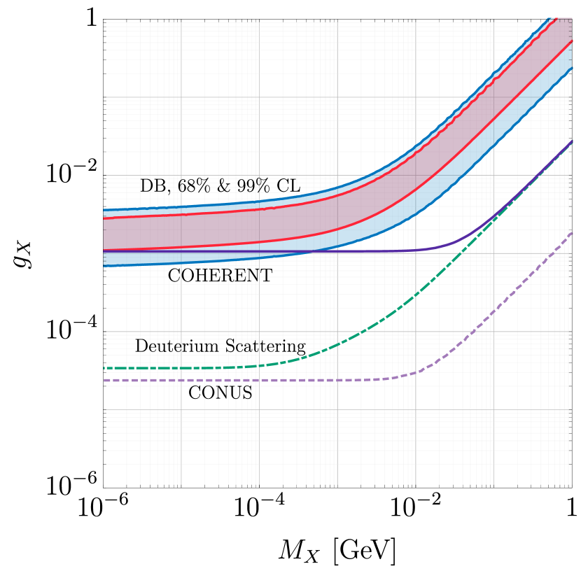
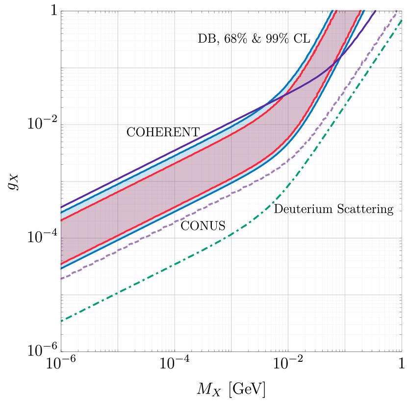
The red (blue) band in fig. 3 represents the 68% (99%) confidence level (CL) from Daya Bay data derived by the analysis described in the previous section, after marginalizing over the power-law index $I$. In our analysis, we have chosen $Y_{n}=-0.65$ and $Y_{\nu}=10$. Constraints from pion decay ($\pi^{0}\to\gamma\,+$ invisible) [36, 37, 38] imply $g_{X}\gtrsim 10^{-2}$ for $M_{X}<m_{\pi}$ and depend on neither $Y_{n}$ nor $Y_{\nu}$; as long as the perturbativity condition $Y_{\nu}\,g_{X}<4\pi$ is maintained, the new neutrino charge can be arbitrarily large. Choosing $Y_{\nu}=10$ allows us to circumvent these constraints. Moreover, there exist strong bounds on this scenario from ²⁰⁸Pb-n scattering [39, 40]. These bounds, however, can be evaded by judiciously choosing the neutron charge to minimize the charge of ²⁰⁸Pb under this interaction; the choice $Y_{n}=-0.65$ allows us to do precisely this. We have also considered bounds from kaon decay [41, 42, 43, 44] and from fifth-force searches [27, 28]; these do not provide particularly stringent additional constraints.

The most relevant bounds on this model derive from neutrino scattering experiments. We show three such constraints in fig. 3: bounds from COHERENT [9] (purple), CONUS [45] (dashed violet) and deuterium scattering [10] (dot-dashed green). While COHERENT leaves a portion of the preferred Daya Bay region unconstrained, the measurement of the deuterium disintegration fully excludes this model. In the near future, this exclusion is expected to be even stronger, once the results of the CONUS experiment, which is probing coherent neutrino-nucleus scattering at a reactor source, are released.

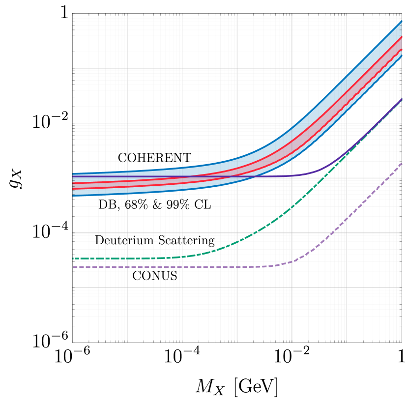
In fig. 4, we show the results of a similar analysis to fig. 3, except transitions to the ground state of ¹²C are included without suppression. While more of the parameter space preferred by Daya Bay lies beyond the exclusion reach of COHERENT, we do not regard this as a genuine improvement over fig. 3 for two reasons. (1) The overall quality of the fit is poorer. The minimum chi-squared, $\chi^{2}_{\rm min}$, is 16.8 here, whereas this value is 9.1 when transitions to the ground state are removed. This is because the fit prioritizes the low-energy upturn over the bump at 5 MeV, as mentioned above. (2) The power-law index $I$ preferred by the fit is smaller ($I\sim 7$ vs. $I\sim 13$), indicating a preference for a harder antineutrino spectrum at high energies. We have not formally constrained this high-energy component in our fit, but preliminary data [16] suggest that this is inconsistent with Daya Bay observations. Therefore, we will continue to ignore transitions to the ground state of ¹²C for the rest of this work.

In what follows, we briefly discuss our treatment of coherent elastic neutrino-nucleus scattering (CE$\nu$NS) and neutrino-induced deuteron disintegration.

COHERENT and CONUS

The differential cross section for CE$\nu$NS involving $\nu_{\alpha}$ (or $\overline{\nu}_{\alpha}$) is

$$\frac{d\sigma_{\alpha}}{dE_{r}}=\frac{G_{F}^{2}}{\pi}|Q_{\alpha}|^{2}F^{2}(q^{2})M\left(1-\frac{ME_{r}}{2E_{\nu}^{2}}\right),$$ (13)

where $E_{\nu}$ is the neutrino energy, $G_{F}$ is Fermi’s constant, $M$ is the mass of target nucleus with $N$ neutrons and $Z$ protons, $q^{2}\approx-2ME_{r}$ is the momentum transfer that gives rise to nuclear recoil energy $E_{r}$, $F^{2}(q^{2})$ is the Helm form factor [46] and $Q_{\alpha}$ is the species-dependent effective charge. In the Standard Model, $Q_{\alpha}$ is given by

$$Q_{\alpha}=Zg_{p}^{V}+Ng_{n}^{V},$$ (14)

where $g_{p}^{V}\,=\frac{1}{2}-2\sin^{2}\theta_{W}$ and $g_{n}^{V}\,=-\frac{1}{2}$ are the proton and neutron weak vector couplings, respectively, and $\theta_{W}$ is the Weinberg angle. We ignore contributions from the axial part of the weak interactions.

The presence of a light new vector particle induces additional contributions to the effective charge that interfere with the SM. These contributions to $Q_{\alpha}$ are weighted by the relevant oscillation amplitudes. Namely,

$$Q_{\alpha}= \,\,\mathcal{A}_{\alpha\alpha}(Zg_{p}^{V}+Ng_{n}^{V})$$

$$+\mathcal{A}_{\alpha s}\left(\frac{-\sqrt{2}g_{X}^{2}Y_{\nu,\overline{\nu}}(Z+Y_{n}N)}{2G_{F}(M_{X}^{2}+2ME_{r})}\right),$$ (15)

where $Y_{\nu,\overline{\nu}}$ is either the neutrino or antineutrino charge, as appropriate; $\mathcal{A}_{\alpha\alpha}$ is the amplitude for $\nu_{\alpha}$ disappearance; and $\mathcal{A}_{\alpha s}$ is the amplitude for $\nu_{s}$ appearance in a $\nu_{\alpha}$ beam. In the limit in which oscillations among the SM neutrinos are irrelevant, the oscillation amplitudes are

$$\mathcal{A}_{\alpha\alpha} =1-2i\exp\left({\frac{-i\Delta m^{2}_{41}L}{4E_{\nu}}}\right)\sin^{2}\theta_{\alpha\alpha}\sin\left({\frac{\Delta m^{2}_{41}L}{4E_{\nu}}}\right)$$ (16)

$$\mathcal{A}_{\alpha s} =2i\exp\left({\frac{-i\Delta m^{2}_{41}L}{4E_{\nu}}}\right)\cos\theta_{\alpha\alpha}\sin\theta_{\alpha\alpha}\sin\left({\frac{\Delta m^{2}_{41}L}{4E_{\nu}}}\right),$$ (17)

where $\sin^{2}\theta_{\alpha\alpha}\equiv|U_{\alpha 4}|^{2}$. Squaring this yields

$$|Q_{\alpha}|^{2}= \,\,P_{\alpha\alpha}\times\left(Zg_{p}^{V}+Ng_{n}^{V}\right)^{2}$$

$$+P_{\alpha s}\times\left(\frac{-\sqrt{2}g_{X}^{2}Y_{\nu,\overline{\nu}}(Z+Y_{n}N)}{2G_{F}(M_{X}^{2}+2ME_{r})}\right)^{2}$$

$$+2\sin 2\theta_{\alpha\alpha}\cos 2\theta_{\alpha\alpha}\sin^{2}\left(\frac{\Delta m_{41}^{2}L}{4E_{\nu}}\right)\times$$

$$\left(Zg_{p}^{V}+Ng_{n}^{V}\right)\left(\frac{-\sqrt{2}g_{X}^{2}Y_{\nu,\overline{\nu}}(Z+Y_{n}N)}{2G_{F}(M_{X}^{2}+2ME_{r})}\right),$$ (18)

where the oscillation probabilities are given by

$$P_{\alpha s}=1-P_{\alpha\alpha}=\sin^{2}2\theta_{\alpha\alpha}\sin^{2}\left(\frac{\Delta m_{41}^{2}L}{4E_{\nu}}\right).$$ (19)

We emphasize that the only nonzero new mixing parameter that we consider is $\sin^{2}2\theta_{ee}$, i.e., muon neutrinos do not mix with the fourth flavor.

We wish to determine the exclusion reach of COHERENT and the sensitivity of CONUS. We simulate COHERENT following the procedure described in Refs. [47, 48]; for CONUS, we follow Ref. [48]. For most values of $Y_{n}$, COHERENT excludes most of Daya Bay’s preferred parameter space. However, choosing the neutron charge to minimize the $U(1)_{X}$ charges of the constituent nuclei allows for the bound to be loosened by a factor of $\sim 10$. Since the relevant isotopes for COHERENT are ¹³³Cs and ¹²⁷I, $Y_{n}=-0.65$ – which we had previously chosen to evade ²⁰⁸Pb-n scattering constraints – provides modest relief (see eq. 12).

We show the 99% CL exclusion limit for COHERENT in purple in fig. 3. If we had selected the best-fit point from Ref. [35], $(\Delta m_{41}^{2},\,\sin^{2}2\theta_{ee})\sim(1.3\text{ eV}^{2},\,0.04)$, then COHERENT would have ruled out the entire region preferred by Daya Bay. Given COHERENT’s characteristic neutrino energy ($\sim\mathcal{O}(30)$ MeV) and baseline (19.3 m), the event rate approximately scales as $g_{X}^{4}\sin^{2}2\theta_{ee}(\Delta m_{41}^{2})^{2}$ for $\Delta m_{41}^{2}\lesssim 0.5$ eV². The COHERENT constraint is weakened as $\Delta m^{2}_{41}$ is decreased, but our willingness to do so in order to avoid this constraint is dictated by reactor data [35]. Our benchmark parameters – $(\Delta m_{41}^{2},\,\sin^{2}2\theta_{ee})\sim(0.4\text{ eV}^{2},\,0.04)$ – are allowed at 95% CL by Ref. [35] and permit us to marginally evade this constraint.

While the sensitivity of COHERENT is slightly diminished for $Y_{n}=-0.65$, the CONUS detector is made of natural germanium, for which the proton-to-neutron ratio is $\sim 0.8$. Consequently, each of the five naturally-occurring germanium isotopes has nonzero charge under $U(1)_{X}$, so it is not possible to simultaneously provide relief from both Pb-n scattering and COHERENT constraints while also limiting the sensitivity of CONUS. The 99% CL sensitivity of CONUS is shown in dashed violet in fig. 3.

Neutrino-induced deuterium disintegration

With the COHERENT limit not fully excluding the preferred Daya Bay region, and with CONUS not yet having released any results, only the bound from the neutrino-induced deuterium disintegration currently rules out the exchange of a vector boson. We briefly discuss how this limit has been calculated.

We have calculated the contributions of our NP model to the cross section for inelastic neutrino-deuterium scattering at reactors, following the calculations of Refs. [49, 50]. In appendix A, we outline the computation of the cross section in the SM and demonstrate how the effects from NP can be included.

To obtain the limit, we first calculate the flux-weighted cross section at 11.2 m from a nuclear reactor, as in Ref. [10], for our benchmark fourth neutrino parameters using the HM fluxes for a range of $g_{X}$ and $M_{X}$. The results are then compared against the same for the purely SM case. Ref. [10] reports a measurement of the $\overline{\nu}$ scattering rate consistent with the SM value at the $\sim 10\%$ level; this allows us to exclude parts of the $\{g_{X},\,M_{X}\}$ parameter space. In fig. 3, we show in light green the contour along which $\tilde{\sigma}^{\rm SM+NP}=2\tilde{\sigma}^{\rm SM}$ in the $\{g_{X},\,M_{X}\}$ plane, where $\tilde{\sigma}^{\rm SM}$ ($\tilde{\sigma}^{\rm SM+NP}$) is the SM (SM+NP) flux-weighted cross section; this is intended to be a conservative limit, given the complexity of the underlying measurement. This result clearly excludes the vector-boson-exchange explanation of the reactor antineutrino excess.

IV.2 Axial interaction

Next, we consider a spin-1 boson $X$ with purely axial couplings to the fourth neutrinos and to nucleons,

$$\mathcal{L}\supset g_{X}X_{\mu}\left(Y_{\nu}\overline{\nu}_{s}\gamma^{\mu}\gamma_{5}\nu_{s}+\overline{p}\gamma^{\mu}\gamma_{5}p+Y_{n}\overline{n}\gamma^{\mu}\gamma_{5}n\right)\,.$$ (20)

Integrating out $X$ leads to the effective Lagrangian of the form

$$\mathcal{L}\supset\frac{-g_{X}^{2}Y_{\nu}}{q^{2}-M_{X}^{2}}\left(\overline{\nu}_{s}\gamma^{\mu}P_{L}\nu_{s}\right)\left(\overline{p}\gamma_{\mu}\gamma_{5}p+Y_{n}\overline{n}\gamma_{\mu}\gamma_{5}n\right),$$ (21)

where we have selected the left-handed part of the neutrino current because any neutrino present in an experiment will arise from a neutrino (antineutrino) produced in weak-interaction processes and will thus be initially left-handed (right-handed), to leading order.

Naively, an axial-vector interaction may be able to relax constraints from COHERENT and CONUS; for similar vector and axial couplings to nucleons, the axial contribution to the cross section is roughly a factor of $1/A$ smaller than its vector counterpart [51, 52]. Hence, if the NP vector couplings were to vanish, then the axial interaction may be significantly less constrained than a comparably-sized vector interaction. We have performed such an analysis and have found a factor of few relaxation of the $g_{X}$ limit. This qualitatively does not alter the picture given in section IV.1. It is interesting to note that it is possible to make either the COHERENT (CONUS) bound vanish, at leading order, by demanding the proton (neutron) to be uncharged under this new axial interaction.

Despite the more positive outlook at CE$\nu$NS experiments compared to the pure vector interaction, the bound from deuterium disintegration turns out to be stronger than its vector-interaction counterpart. We do not review here the full derivation, but point the interested reader to appendix A, where the treatment for the vector interaction is outlined. We emphasize that only the coefficients representing the axial-vector isoscalar and isovector couplings $(C_{A}^{(0)},C_{A}^{(1)})$ get modified in this case. As mentioned previously, a full calculation of the ¹³C$(\overline{\nu},\overline{\nu}^{\prime}n)^{12}$C^(∗) cross section for an axial-vector mediator is well beyond the scope of this work. However, it is likely that neutrino-induced deuterium disintegration would place a cripplingly strong bound on such a scenario.

IV.3 Magnetic interaction

Lastly, we consider a magnetic-magnetic interaction between the new neutrinos and nuclei. We introduce an effective interaction of the form

$$\mathcal{L}\supset\sum_{N=p,\,n}\frac{\mu_{\nu}\mu_{N}}{q^{2}-M_{X}^{2}}\left(\overline{\nu}_{s}\sigma^{\mu\nu}(iq_{\nu})\nu_{s}\right)\left(\overline{N}\sigma_{\mu\alpha}(iq^{\alpha})N\right),$$ (22)

where $\mu_{\nu}$ and $\mu_{N}$ are the neutrino and nucleon magnetic dipole moments, respectively. We parameterize the latter as $\mu_{N}=g_{X}\mu^{\rm SM}_{N}$, where $\mu^{\rm SM}_{N}$ is the SM magnetic dipole moment with the fundamental charge $e$ factored out ($\mu^{\rm SM}_{p}=2.79/2m_{N}$ and $\mu^{\rm SM}_{n}=-1.91/2m_{N}$). The neutrino magnetic moment is defined to be $\mu_{\nu}\equiv g_{X}Y_{\nu}/M_{X}$.

To estimate the constraint from Daya Bay, we follow the example of Ref. [53], wherein the $\overline{\nu}d\to\overline{\nu}np$ cross section is calculated for nonzero neutrino magnetic moments using the $\gamma d\to np$ cross section to sidestep complications arising from nuclear structure. Of course, the ¹³C$(X,n)^{12}$C^(∗) cross section is not measured; we use the ¹³C$(\gamma,n)^{12}$C^(∗) cross section instead [54] modified by a factor of $\frac{2}{3}(g_{X}/e)^{2}$, to account for (1) the difference in coupling strengths, and (2) the difference in the number of allowed spin states of our massive vector boson. This forces us into assuming that the longitudinal mode of our massive boson would not contribute appreciably to ¹³C$(X,n)^{12}$C^(∗). The experimentally determined total ¹³C$(\gamma,n)^{12}$C^(∗) cross section does not reveal how much of this cross section comes from M1 scattering and how much from E1 scattering. We assume that M1 scattering dominates; if this is untrue, then the Daya Bay data will prefer larger values of $g_{X}$ than this optimistic analysis.

With these assumptions and by following Ref. [53], we obtain the following differential cross section:

$$\frac{d\sigma}{dE^{\prime}}=\frac{\mu_{\nu}^{2}g_{X}^{2}(E-E^{\prime})E^{\prime}\times\sigma_{\gamma}(E_{\gamma}=E-E^{\prime})}{4\pi^{3}\alpha E(M_{X}^{2}+2(E-E^{\prime})^{2})(M_{X}^{2}+4EE^{\prime})}\times\Big{[}4EE^{\prime}(M_{X}^{2}+2EE^{\prime})-M_{X}^{2}(M_{X}^{2}+4EE^{\prime})\log\left(\frac{M_{X}^{2}+4EE^{\prime}}{M_{X}^{2}}\right)\Big{]}\,,$$ (23)

where $E$ ($E^{\prime})$ is the initial (final) antineutrino energy and $\sigma_{\gamma}$ is the ¹³C$(\gamma,n)^{12}$C^(∗) cross section. Note that the final neutrino energy satisfies $E^{\prime}=E-S_{n}-E_{\rm ex}-E_{\rm nuc}$, where $S_{n}$ is the neutron removal energy of ¹³C, $E_{\rm ex}$ is the excitation energy of the final ¹²C (either 0 or $\sim$ 4.4 MeV), and $E_{\rm nuc}$ is the kinetic energy carried off by the ¹²C-neutron system. We assume that the neutron carries off most of this energy and, therefore, that eq. 23 is also the neutron recoil spectrum.

The red (blue) band in fig. 5 is the 68% (99%) confidence level preferred by the Daya Bay data. We include only transitions to the first excited state of ¹²C, and find that $\chi^{2}_{\rm min}$/d.o.f. = 11.7/22 ($p=0.96$). Including transitions to the ground state of ¹²C makes the parameter space preferred by Daya Bay slightly narrower and increases $\chi^{2}_{\rm min}$/d.o.f. $\to$ 16.6/22 ($p=0.78$); the fit still suffers from fitting the low-energy upturn instead of the 5 MeV bump. The no-ground-state fit is slightly poorer than its vector-interaction analog – recall that we had found $\chi^{2}_{\rm min}$/d.o.f. = 9.1/22 – but it remains to determine the extent to which CE$\nu$NS and deuterium disintegration experiments can exclude such scenario, as in sections IV.1 and IV.2.

For the CE$\nu$NS cross section, we extend the formalism for nonrelativistic dark matter-nucleon effective field theory presented in Refs. [55, 56] to account for the fact that neutrinos are ultrarelativistic; a detailed calculation will be presented in Ref. [57]. We have verified that we recover the usual CE$\nu$NS cross section from this framework in the absence of NP. The result is similar to the one presented in section IV.1 for a vector interaction. In fig. 5, we see that COHERENT (purple) does little to challenge the parameter space preferred by Daya Bay. We have shown the result for our benchmark fourth neutrino parameters, in the interest of consistency, but have determined that even for the best-fit point of Ref. [35], having a larger $\Delta m_{41}^{2}$ ( = 1.3 eV²), COHERENT provides only a modest exclusion of the high-mass ($M_{X}\gtrsim 10$ MeV) portion of the Daya Bay preferred region. However, CONUS (dashed violet) will have the power to fully exclude this model.

For deuterium disintegration, we repurpose the results of Ref. [58] to determine the cross section. We use a modified version of the M1 matrix element given in their eq. (11), to account for differences in normalization convention and the effects of a nonzero $M_{X}$:

$$|M|^{2}= \,\,|\mathcal{M_{\rm nuc}}|^{2}g_{X}^{2}(\mu^{\rm SM}_{p}-\mu^{\rm SM}_{n})^{2}\mu_{\nu}^{2}\times$$ (24)

$$EE_{f}\left(\frac{1+\mathbf{n_{1}}\cdot\mathbf{n_{2}}}{3}\right)\times(2m_{N})^{3}\left(\frac{q^{2}}{q^{2}-M_{X}^{2}}\right)^{2},$$

where $\mathbf{n_{1}}$ ($\mathbf{n_{2}}$) is the unit vector along the direction of the incident (outgoing) neutrino, which respectively have energies $E$ and $E_{f}$. Ref. [58] only includes the isovector contributions to the scattering cross section because these would ultimately dominate. Additionally, $|\mathcal{M_{\rm nuc}}|^{2}$ incorporates the effects of the structure of deuterium; it is given by Eq. (12) of Ref. [58] and depends on $E_{k}$, the kinetic energy of the relative motion of the final-state proton and neutron.

Figure 5: Bounds on the magnetic-interaction scenario from COHERENT (solid purple), CONUS (dashed violet) and deuterium disintegration (dot-dashed green), as described in the text. We continue to take $\Delta m_{41}^{2}=0.4$ eV², $\sin^{2}2\theta=0.04$ and $Y_{\nu}=+10$. Here, we include only transitions to the first excited state of ¹²C in our analysis of Daya Bay.

The differential cross section reads

$$\frac{d\sigma}{dE_{k}}=\frac{|\mathcal{M}|^{2}g_{X}^{4}Y_{\nu}^{2}\mu_{\rm SM}^{2}(E-B-E_{k})^{2}\sqrt{E_{k}}}{384\pi^{3}\sqrt{m_{N}}M_{X}^{2}}f(z)\,,$$ (25)

where $\mu_{\rm SM}\equiv 2m_{N}(\mu^{\rm SM}_{p}-\mu^{\rm SM}_{n})$ is the isovector nucleon magnetic moment, $m_{N}$ is the nucleon mass and $B$ is deuteron binding energy. The function $f(z)$ reads

$$f(z)\equiv\int^{1}_{-1}dx\frac{(1+x)(1-x)^{2}}{(1+z-x)^{2}}=$$ (26)

$$2+6z-2z(4+3z)\coth^{-1}(1+z)\,,$$ (27)

where we define $z\equiv M_{X}^{2}/(2EE_{f})$.

From eq. 25, it is straightforward to calculate the flux-weighted cross section and obtain the limit in a similar fashion as described at the end of section IV.1. From fig. 5, we observe that the deuterium disintegration limit (dot-dashed green) again rules out the entirety of the parameter space preferred by Daya Bay. Hence, this model is strongly disfavored.

V Summary and Conclusions

In this work, we have studied whether the 5 MeV neutrino excess at reactors can be addressed with physics beyond the SM — more precisely, via the interplay between nuclear physics and new particle physics. By injecting at least $9.4$ MeV of energy into the nucleus, ¹³C may transition to the lowest-lying excited state of ¹²C which subsequently de-excites. The resulting $4.4$ MeV photon, together with energy deposited during neutron thermalization, can successfully explain the excess. We introduced additional, eV-scale neutrinos and assumed them to have hidden interactions with nucleons to allow them to scatter off of ¹³C nuclei.

We considered three minimal types of the interactions: vector, axial and magnetic. In all cases, the parameter space preferred by Daya Bay is excluded by neutrino-induced deuterium disintegration, is in severe tension with the data collected by COHERENT and will be strongly challenged by CONUS data in the near future. While non-minimal NP scenarios could explain the reactor bump, this work suggests that the antineutrino excess in the reactor data is more likely to be of nuclear physics origin.

Interestingly, is possible to probe whether or not ¹³C$(\overline{\nu},\overline{\nu}^{\prime}n)^{12}$C^∗ is responsible for the reactor bump in a model-independent way. This reaction is available at all organic scintillator detectors (liquid or solid) and the prompt signal is a combination of proton recoils (about 20%) and the 4.4 MeV de-excitation photon. In single-volume detectors like Daya Bay and NEOS, the 4.4 MeV photon is well contained; neither employs pulse shape discrimination, so these events pass as genuine IBD events. PROSPECT [59, 60, 61] and STEREO [62, 63, 64] both rely on pulse shape discrimination to manage backgrounds, so the small proton recoil contribution will likely cause these events to be rejected as background. Also, the 4.4 MeV photon would deposit energy across many detector cells; it seems likely that no bump would be observed in the standard analysis. The relatively long distance over which the 4.4 MeV photon deposits its energy, compared to a positron in an IBD event, is likely to have these events rejected in finely segmented detectors like SoLid [65] and DANSS [66, 67]. Curiously, DANSS seems not to observe a bump, in accordance with this prediction. A dedicated analysis in these segmented detectors could likely identify this process.

The analogous reaction ¹⁷O$(\bar{\nu},\bar{\nu}^{\prime}n)^{16}$O^∗ is unlikely to be observed at water Cerenkov detectors. First, the natural abundance of ¹⁷O ($0.03\%$) is significantly lower than that of ¹³C ($1.07\%$). Second, while the neutron separation energy of ¹⁷O (4143.1 keV) is slightly less than that of ¹³C, the lowest-lying excited state of ¹⁶O has an excitation energy of 6049.6 keV [70]; populating this state would require a significant antineutrino flux beyond $E_{\nu}\gtrsim 10$ MeV, and we have seen that this flux dies off quite quickly. Even though this could, in principle, give rise to an analogous bump in the prompt energy spectrum at $\sim 6$ MeV in water Cerenkov detectors, it would be substantially more difficult to detect. Therefore, neither Gd-doped Super-K [71] nor WATCHMAN [72] should see a bump.

Acknowledgments. The authors would like to thank Evgeny Akhmedov, Giorgio Arcadi, Phil Barbeau, Omar Benhar, Thomas O’Donnell, Joerg Jaeckel, Joachim Kopp, Stefan Vogl and Xun-Jie Xu for useful discussions. The authors further thank Alexei Smirnov and Petr Vogel for bringing deuterium disintegration results to our attention. The work of JB and PH is supported by the U.S. Department of Energy under award number DE-SC0018327.

Appendix A Deuterium disintegration cross section

The cross section for neutrino-deuterium scattering can be written [49, 50]

$$\frac{d^{2}\sigma}{dE_{f}d\Omega_{f}}= \,\,\frac{G_{F}^{2}E_{f}^{2}}{2\pi^{2}}\times$$ (28)

$$\left[2W_{1}^{\rm LO}\sin^{2}\frac{\theta_{f}}{2}+(W_{0}^{\rm LO}+W_{1}^{\rm LO})\cos^{2}\frac{\theta_{f}}{2}\right],$$

where $E_{f}$ and $\Omega_{f}$ are the final-state neutrino energy and solid angle, respectively. The functions $W_{0}^{\rm LO}$ and $W_{1}^{\rm LO}$ are hadronic structure functions, calculated in Refs [49, 50]. For completeness, we list the functions that enter into this cross section:

$$W_{0}^{\rm LO}= \,\,2\left(|C_{V}^{(0)}|^{2}+|C_{V}^{(1)}|^{2}\right)F_{1}$$

$$+\left(|C_{V}^{(0)}|^{2}-|C_{V}^{(1)}|^{2}\right)F_{2}$$ (29)

$$+4|C_{V}^{(0)}|^{2}F^{\rm LO}_{3},$$

$$W_{1}^{\rm LO}= \,\,2\left(|C_{A}^{(0)}|^{2}+|C_{A}^{(1)}|^{2}\right)F_{1}$$

$$+\frac{1}{3}\left(|C_{A}^{(0)}|^{2}-|C_{A}^{(1)}|^{2}\right)F_{2}$$ (30)

$$+\frac{8}{3}|C_{A}^{(0)}|^{2}F^{\rm LO}_{3}+\frac{4}{3}|C_{A}^{(1)}|^{2}F^{\rm LO}_{4},$$

$$F_{1}= \,\,\frac{2M_{N}\gamma p}{\pi(p^{2}+\gamma^{2})^{2}}\left(1+\frac{|{\mathbf{q}}|^{2}(p^{2}-\gamma^{2})}{2(p^{2}+\gamma^{2})^{2}}\right),$$ (31)

$$F_{2}= \,\,\frac{4M_{N}\gamma p}{\pi(p^{2}+\gamma^{2})^{2}}\left(1-\frac{|{\mathbf{q}}|^{2}(p^{2}+3\gamma^{2})}{6(p^{2}+\gamma^{2})^{2}}\right),$$ (32)

$$F_{3}= \,\,\frac{1}{\pi}\Im\left[B_{0}(p,|{\mathbf{q}}|)^{2}A_{-1}^{(^{3}S_{1})}\right],$$ (33)

$$F_{4}= \,\,\frac{1}{\pi}\Im\left[B_{0}(p,|{\mathbf{q}}|)^{2}A_{-1}^{(^{1}S_{0})}\right],$$ (34)

$$B_{0}(p,|{\mathbf{q}}|)= \,\,-\sqrt{\frac{\gamma}{2\pi}}\frac{M_{N}}{\gamma-ip}\left(1-\frac{|{\mathbf{q}}|^{2}}{12(\gamma-ip)^{2}}\right),$$ (35)

$$A_{-1}^{(^{3}S_{1})}= \,\,-\frac{4\pi}{M_{N}}\frac{1}{\gamma+ip},$$ (36)

$$A_{-1}^{(^{1}S_{0})}= \,\,-\frac{4\pi}{M_{N}}\frac{a^{(^{1}S_{0})}}{1+ip\,a^{(^{1}S_{0})}},$$ (37)

$$p= \,\,\sqrt{M_{N}\nu-\gamma^{2}-\frac{|{\mathbf{q}}|^{2}}{4}+i\epsilon}\quad(\epsilon\to 0^{+}),$$ (38)

$$|{\mathbf{q}}|^{2}= \,\,{\nu^{2}+4E_{i}E_{f}\sin^{2}\frac{\theta_{f}}{2}},$$ (39)

$$\nu= \,\,E_{i}-E_{f},$$ (40)

$$\gamma= \,\,\sqrt{M_{N}B}.$$ (41)

In these formulae, $M_{N}\approx 938$ MeV is the nucleon mass, $B=2.2245$ MeV is the deuteron binding energy, $a^{(^{1}S_{0})}=-23.7$ fm is the deuteron scattering length, $C_{V,A}^{(0)}$ is the vector/axial-vector isoscalar coupling and $C_{V,A}^{(1)}$ is the vector/axial-vector isovector coupling. The SM couplings are given by

$$C^{(0)}_{V,\text{SM}}= \,\,-\sin^{2}\theta_{W},$$ (42)

$$C^{(1)}_{V,\text{SM}}= \,\,\frac{1}{2}\left(1-2\sin^{2}\theta_{W}\right),$$ (43)

$$C^{(0)}_{A,\text{SM}}= \,\,-\frac{1}{2}\Delta s,$$ (44)

$$C^{(1)}_{A,\text{SM}}= \,\,\frac{1}{2}g_{A},$$ (45)

where $\theta_{W}$ is the Weinberg angle, $\Delta s$ is the strange-quark contribution to the proton spin and $g_{A}$ is the $\pi NN$ coupling constant.

The new vector interaction we introduce induces additional contributions to $C_{V}^{(I=0,1)}$. Starting from the effective Lagrangian

$$\mathcal{L}\supset \,\,\frac{g_{X}^{2}Y_{\nu}}{q^{2}-M_{X}^{2}}\left(\overline{\nu}_{s}\gamma^{\mu}\nu_{s}\right)\left(\overline{p}\gamma_{\mu}p+Y_{n}\overline{n}\gamma_{\mu}n\right),$$ (46)

we determine the NP isoscalar and isovector couplings to be

$$C^{(0)}_{V,\text{NP}}= \,\,\frac{\sqrt{2}g_{X}^{2}Y_{\overline{\nu}}(1+Y_{n})}{4G_{F}(M_{X}^{2}+4E_{i}E_{f}\sin^{2}\frac{\theta_{f}}{2})},$$ (47)

$$C^{(1)}_{V,\text{NP}}= \,\,\frac{-\sqrt{2}g_{X}^{2}Y_{\overline{\nu}}(1-Y_{n})}{4G_{F}(M_{X}^{2}+4E_{i}E_{f}\sin^{2}\frac{\theta_{f}}{2})},$$ (48)

where we have used that $q^{2}=-4E_{i}E_{f}\sin^{2}\frac{\theta_{f}}{2}$. Note that a negative sign has been absorbed via $Y_{\overline{\nu}}=-Y_{\nu}$. We incorporate the SM and NP by adding $C^{(I)}_{V,\text{SM}}$ and $C^{(I)}_{V,\text{NP}}$, weighted by the relevant oscillation amplitude:

$$C_{V}^{(I)}=\mathcal{A}_{ee}C^{(I)}_{V,\text{SM}}+\mathcal{A}_{es}C^{(I)}_{V,\text{NP}}\,,$$ (49)

where we need only to consider oscillations involving electron (anti)neutrinos. Squaring this and using the expressions in eqs. 16 and 17, leads to

$$|C_{V}^{(I)}|^{2}= \,\,P_{ee}\left(C^{(I)}_{V,\text{SM}}\right)^{2}+P_{es}\left(C^{(I)}_{V,\text{NP}}\right)^{2}$$ (50)

$$+2\sin 2\theta_{ee}\cos 2\theta_{ee}\sin^{2}\left(\frac{\Delta m_{41}^{2}L}{4E_{\nu}}\right)\times$$

$$\qquad\left(C^{(I)}_{V,\text{SM}}C^{(I)}_{V,\text{NP}}\right).$$

To calculate the total cross section, eq. 28 must be integrated over the region

$$E_{f}\in \,\,\left[0,E_{i}-2\left(M_{N}-\sqrt{M_{N}^{2}-\gamma^{2}}\right)\right],$$ (51)

$$\cos\theta_{f}\in \,\,\left[\text{Max}\left[-1,1-\frac{4M_{N}(\nu-B)-\nu^{2}}{2E_{i}E_{f}}\right],1\right],$$ (52)

$$\varphi_{f}\in \,\,\left[0,2\pi\right].$$ (53)

References

- Abe et al. [2012] Y. Abe et al. (Double Chooz), “Indication of Reactor Disappearance in the Double Chooz Experiment,” Phys. Rev. Lett. 108, 131801 (2012), eprint 1112.6353.
- An et al. [2012] F. P. An et al. (Daya Bay), “Observation of electron-antineutrino disappearance at Daya Bay,” Phys. Rev. Lett. 108, 171803 (2012), eprint 1203.1669.
- Ahn et al. [2012] J. K. Ahn et al. (RENO), “Observation of Reactor Electron Antineutrino Disappearance in the RENO Experiment,” Phys. Rev. Lett. 108, 191802 (2012), eprint 1204.0626.
- Mention et al. [2011] G. Mention, M. Fechner, T. Lasserre, T. A. Mueller, D. Lhuillier, M. Cribier, and A. Letourneau, “The Reactor Antineutrino Anomaly,” Phys. Rev. D83, 073006 (2011), eprint 1101.2755.
- Huber [2016] P. Huber, “Reactor antineutrino fluxes – Status and challenges,” Nucl. Phys. B908, 268 (2016), eprint 1602.01499.
- Huber [2017] P. Huber, “NEOS Data and the Origin of the 5 MeV Bump in the Reactor Antineutrino Spectrum,” Phys. Rev. Lett. 118, 042502 (2017), eprint 1609.03910.
- Buck et al. [2017] C. Buck, A. P. Collin, J. Haser, and M. Lindner, “Investigating the Spectral Anomaly with Different Reactor Antineutrino Experiments,” Phys. Lett. B765, 159 (2017), eprint 1512.06656.
- Dwyer and Langford [2015] D. A. Dwyer and T. J. Langford, “Spectral Structure of Electron Antineutrinos from Nuclear Reactors,” Phys. Rev. Lett. 114, 012502 (2015), eprint 1407.1281.
- Akimov et al. [2017] D. Akimov et al. (COHERENT), “Observation of Coherent Elastic Neutrino-Nucleus Scattering,” Science 357, 1123 (2017), eprint 1708.01294.
- Reines et al. [1980] F. Reines, H. W. Sobel, and E. Pasierb, “Evidence for Neutrino Instability,” Phys. Rev. Lett. 45, 1307 (1980).
- Suzuki et al. [1999] S. Suzuki, T. Saito, K. Takahisa, C. Takakuwa, T. Nakagawa, T. Tohei, and K. Abe, “Neutron decay of the pygmy and giant resonances in the reaction,” Phys. Rev. C60, 034309 (1999).
- An et al. [2017] F. P. An et al. (Daya Bay), “Improved Measurement of the Reactor Antineutrino Flux and Spectrum at Daya Bay,” Chin. Phys. C41, 013002 (2017), eprint 1607.05378.
- Huber [2011] P. Huber, “On the determination of anti-neutrino spectra from nuclear reactors,” Phys. Rev. C84, 024617 (2011), [Erratum: Phys. Rev.C85,029901(2012)], eprint 1106.0687.
- Mueller et al. [2011] T. A. Mueller et al., “Improved Predictions of Reactor Antineutrino Spectra,” Phys. Rev. C83, 054615 (2011), eprint 1101.2663.
- Fallot et al. [2012] M. Fallot et al., “New antineutrino energy spectra predictions from the summation of beta decay branches of the fission products,” Phys. Rev. Lett. 109, 202504 (2012), eprint 1208.3877.
- Raper [2016] N. Raper, Ph.D. thesis, Rensselaer Polytechnic Institute (2016).
- Hayes et al. [2015] A. C. Hayes, J. L. Friar, G. T. Garvey, D. Ibeling, G. Jungman, T. Kawano, and R. W. Mills, “Possible origins and implications of the shoulder in reactor neutrino spectra,” Phys. Rev. D92, 033015 (2015), eprint 1506.00583.
- Birks [1951] J. B. Birks, “Scintillations from Organic Crystals: Specific Fluorescence and Relative Response to Different Radiations,” Proc. Phys. Soc. A64, 874 (1951).
- [19] Y. Minfeng, private communication.
- pst [1993] Tech. Rep. 49, International Commission on Radiation Units and Measurements (1993).
- Ko et al. [2017] Y. Ko et al., “Sterile Neutrino Search at the NEOS Experiment,” Phys. Rev. Lett. 118, 121802 (2017), eprint 1610.05134.
- Maltoni and Schwetz [2003] M. Maltoni and T. Schwetz, “Testing the statistical compatibility of independent data sets,” Phys. Rev. D68, 033020 (2003), eprint hep-ph/0304176.
- Nelson and Scholtz [2011] A. E. Nelson and J. Scholtz, “Dark Light, Dark Matter and the Misalignment Mechanism,” Phys. Rev. D84, 103501 (2011), eprint 1105.2812.
- Buchmuller et al. [1991] W. Buchmuller, C. Greub, and P. Minkowski, “Neutrino masses, neutral vector bosons and the scale of breaking,” Phys. Lett. B267, 395 (1991).
- Khalil [2010] S. Khalil, “TeV-scale gauged B-L symmetry with inverse seesaw mechanism,” Phys. Rev. D82, 077702 (2010), eprint 1004.0013.
- Sahu and Yajnik [2005] N. Sahu and U. A. Yajnik, “Gauged symmetry and baryogenesis via leptogenesis at TeV scale,” Phys. Rev. D71, 023507 (2005), eprint hep-ph/0410075.
- Harnik et al. [2012] R. Harnik, J. Kopp, and P. A. N. Machado, “Exploring Signals in Dark Matter Detectors,” JCAP 1207, 026 (2012), eprint 1202.6073.
- Cerdeño et al. [2016] D. G. Cerdeño, M. Fairbairn, T. Jubb, P. A. N. Machado, A. C. Vincent, and C. Bœhm, “Physics from solar neutrinos in dark matter direct detection experiments,” JHEP 05, 118 (2016), [Erratum: JHEP09,048(2016)], eprint 1604.01025.
- Pospelov [2011] M. Pospelov, “Neutrino Physics with Dark Matter Experiments and the Signature of New Baryonic Neutral Currents,” Phys. Rev. D84, 085008 (2011), eprint 1103.3261.
- Kopp and Welter [2014] J. Kopp and J. Welter, “The Not-So-Sterile 4th Neutrino: Constraints on New Gauge Interactions from Neutrino Oscillation Experiments,” JHEP 12, 104 (2014), eprint 1408.0289.
- Kopp et al. [2013] J. Kopp, P. A. N. Machado, M. Maltoni, and T. Schwetz, “Sterile Neutrino Oscillations: The Global Picture,” JHEP 05, 050 (2013), eprint 1303.3011.
- Gariazzo et al. [2017] S. Gariazzo, C. Giunti, M. Laveder, and Y. F. Li, “Updated Global 3+1 Analysis of Short-BaseLine Neutrino Oscillations,” JHEP 06, 135 (2017), eprint 1703.00860.
- Dentler et al. [2017] M. Dentler, A. Hernández-Cabezudo, J. Kopp, M. Maltoni, and T. Schwetz, “Sterile neutrinos or flux uncertainties? — Status of the reactor anti-neutrino anomaly,” JHEP 11, 099 (2017), eprint 1709.04294.
- Gariazzo et al. [2018] S. Gariazzo, C. Giunti, M. Laveder, and Y. F. Li, “Model-independent short-baseline oscillations from reactor spectral ratios,” Phys. Lett. B782, 13 (2018), eprint 1801.06467.
- Dentler et al. [2018] M. Dentler, . Hernández-Cabezudo, J. Kopp, P. A. N. Machado, M. Maltoni, I. Martinez-Soler, and T. Schwetz, “Updated Global Analysis of Neutrino Oscillations in the Presence of eV-Scale Sterile Neutrinos,” JHEP 08, 010 (2018), eprint 1803.10661.
- Atiya et al. [1992] M. S. Atiya et al., “Search for the decay ,” Phys. Rev. Lett. 69, 733 (1992).
- Batell et al. [2014] B. Batell, P. deNiverville, D. McKeen, M. Pospelov, and A. Ritz, “Leptophobic Dark Matter at Neutrino Factories,” Phys. Rev. D90, 115014 (2014), eprint 1405.7049.
- deNiverville et al. [2015] P. deNiverville, M. Pospelov, and A. Ritz, “Light new physics in coherent neutrino-nucleus scattering experiments,” Phys. Rev. D92, 095005 (2015), eprint 1505.07805.
- Barbieri and Ericson [1975] R. Barbieri and T. E. O. Ericson, “Evidence Against the Existence of a Low Mass Scalar Boson from Neutron-Nucleus Scattering,” Phys. Lett. 57B, 270 (1975).
- Leeb and Schmiedmayer [1992] H. Leeb and J. Schmiedmayer, “Constraint on hypothetical light interacting bosons from low-energy neutron experiments,” Phys. Rev. Lett. 68, 1472 (1992).
- Ecker et al. [1987] G. Ecker, A. Pich, and E. de Rafael, “ Decays in the Effective Chiral Lagrangian of the Standard Model,” Nucl. Phys. B291, 692 (1987).
- Ecker et al. [1988] G. Ecker, A. Pich, and E. de Rafael, “Radiative Kaon Decays and CP Violation in Chiral Perturbation Theory,” Nucl. Phys. B303, 665 (1988).
- D’Ambrosio et al. [1998] G. D’Ambrosio, G. Ecker, G. Isidori, and J. Portoles, “The Decays beyond leading order in the chiral expansion,” JHEP 08, 004 (1998), eprint hep-ph/9808289.
- Pospelov [2009] M. Pospelov, “Secluded U(1) below the weak scale,” Phys. Rev. D80, 095002 (2009), eprint 0811.1030.
- [45] W. Maneschg, “The status of CONUS,”, URL http://doi.org/10.5281/zenodo.1286927.
- Klein and Nystrand [2000] S. R. Klein and J. Nystrand, “Interference in exclusive vector meson production in heavy ion collisions,” Phys. Rev. Lett. 84, 2330 (2000), eprint hep-ph/9909237.
- Liao and Marfatia [2017] J. Liao and D. Marfatia, “COHERENT constraints on nonstandard neutrino interactions,” Phys. Lett. B775, 54 (2017), eprint 1708.04255.
- Farzan et al. [2018] Y. Farzan, M. Lindner, W. Rodejohann, and X.-J. Xu, “Probing neutrino coupling to a light scalar with coherent neutrino scattering,” JHEP 05, 066 (2018), eprint 1802.05171.
- Butler and Chen [2000] M. Butler and J.-W. Chen, “Elastic and inelastic neutrino deuteron scattering in effective field theory,” Nucl. Phys. A675, 575 (2000), eprint nucl-th/9905059.
- Butler et al. [2001] M. Butler, J.-W. Chen, and X. Kong, “Neutrino deuteron scattering in effective field theory at next-to-next-to-leading order,” Phys. Rev. C63, 035501 (2001), eprint nucl-th/0008032.
- Barranco et al. [2005] J. Barranco, O. G. Miranda, and T. I. Rashba, “Probing new physics with coherent neutrino scattering off nuclei,” JHEP 12, 021 (2005), eprint hep-ph/0508299.
- Scholberg [2018] K. Scholberg (COHERENT), in 2017 International Workshop on Neutrinos from Accelerators (NuFact17) Uppsala University Main Building, Uppsala, Sweden, September 25-30, 2017 (2018), eprint 1801.05546, URL https://inspirehep.net/record/1648558/files/arXiv:1801.05546.pdf.
- Grifols et al. [2004] J. A. Grifols, E. Masso, and S. Mohanty, “Neutrino magnetic moments and photodisintegration of deuterium,” Phys. Lett. B587, 184 (2004), eprint hep-ph/0401144.
- Koning and Rochman [2012] A. J. Koning and D. Rochman, “Modern Nuclear Data Evaluation with the TALYS Code System,” Nucl. Data Sheets 113, 2841 (2012).
- Fitzpatrick et al. [2013] A. L. Fitzpatrick, W. Haxton, E. Katz, N. Lubbers, and Y. Xu, “The Effective Field Theory of Dark Matter Direct Detection,” JCAP 1302, 004 (2013), eprint 1203.3542.
- Anand et al. [2014] N. Anand, A. L. Fitzpatrick, and W. C. Haxton, “Weakly interacting massive particle-nucleus elastic scattering response,” Phys. Rev. C89, 065501 (2014), eprint 1308.6288.
- [57] J. M. Berryman, in preparation.
- Akhmedov and Berezin [1992] E. K. Akhmedov and V. V. Berezin, “Neutrino disintegration of deuteron and electromagnetic form-factors of neutrinos,” Z. Phys. C54, 661 (1992).
- Ashenfelter et al. [2016] J. Ashenfelter et al. (PROSPECT), “The PROSPECT Physics Program,” J. Phys. G43, 113001 (2016), eprint 1512.02202.
- Ashenfelter et al. [2019] J. Ashenfelter et al. (PROSPECT), “The PROSPECT Reactor Antineutrino Experiment,” Nucl. Instrum. Meth. A922, 287 (2019), eprint 1808.00097.
- Ashenfelter et al. [2018] J. Ashenfelter et al. (PROSPECT), “First search for short-baseline neutrino oscillations at HFIR with PROSPECT,” Phys. Rev. Lett. 121, 251802 (2018), eprint 1806.02784.
- Manzanillas [2017] L. Manzanillas (STEREO), “STEREO: Search for sterile neutrinos at the ILL,” PoS NOW2016, 033 (2017), eprint 1702.02498.
- Allemandou et al. [2018] N. Allemandou et al. (STEREO), “The STEREO Experiment,” JINST 13, P07009 (2018), eprint 1804.09052.
- Almazán et al. [2018] H. Almazán et al. (STEREO), “Sterile Neutrino Constraints from the STEREO Experiment with 66 Days of Reactor-On Data,” Phys. Rev. Lett. 121, 161801 (2018), eprint 1806.02096.
- Abreu et al. [2018] Y. Abreu et al. (SoLid), “Performance of a full scale prototype detector at the BR2 reactor for the SoLid experiment,” Submitted to: JINST (2018), eprint 1802.02884.
- Alekseev et al. [2016] I. Alekseev et al., “DANSS: Detector of the reactor AntiNeutrino based on Solid Scintillator,” JINST 11, P11011 (2016), eprint 1606.02896.
- Alekseev et al. [2018] I. Alekseev et al. (DANSS), “Search for sterile neutrinos at the DANSS experiment,” Phys. Lett. B787, 56 (2018), eprint 1804.04046.
- [68] D. Svirida, “Searches for sterile neutrinos at the DANSSexperiment,”, URL http://www.ba.infn.it/~now/now2018/assets/svirida_danss_now18.pdf.
- Zacek et al. [2018] V. Zacek, G. Zacek, P. Vogel, and J. L. Vuilleumier, “Evidence for a 5 MeV Spectral Deviation in the Goesgen Reactor Neutrino Oscillation Experiment,” (2018), eprint 1807.01810.
- J.H. Kelley and Cheves [1993] H. W. J.H. Kelley, D.R. Tilley and C. Cheves Nucl. Physics 564, 1 (1993).
- Beacom and Vagins [2004] J. F. Beacom and M. R. Vagins, “GADZOOKS! Anti-neutrino spectroscopy with large water Cherenkov detectors,” Phys. Rev. Lett. 93, 171101 (2004), eprint hep-ph/0309300.
- Askins et al. [2015] M. Askins et al. (WATCHMAN), “The Physics and Nuclear Nonproliferation Goals of WATCHMAN: A WAter CHerenkov Monitor for ANtineutrinos,” (2015), eprint 1502.01132.