Kalman Filter, Unscented Filter and Particle Flow Filter on Non-linear Models

Abstract

Filters, especially wide range of Kalman Filters have shown their impacts on predicting variables of stochastic models with higher accuracy then traditional statistic methods. Updating mean and covariance each time makes Bayesian inferences more meaningful. In this paper, we mainly focused on the derivation and implementation of three powerful filters: Kalman Filter, Unscented Kalman Filter and Particle Flow Filter. Comparison for these different type of filters could make us more clear about the suitable applications for different circumstances.

Chapter 1 Kalman Filter

Kalman Filter, also called the Linear Quadratic Estimator(LQE), has been used to minimize the estimation error for unknown variables in noisy stochastic system. Kalman Filter works recursively to update estimation by inputting observed measurements over time. It contains two models, the first is Observation model and the second is Measurement model. Observation model, involving Plant noise, has been used to generate prior estimation for current state variables; Measurement model, including observation noise, has been used to update the estimation and generate posterior estimation. Kalman Filter has wide applications, such as predicting natural weather and prices of traded commodities. It also has been used to monitor complex dynamic systems, like signal processing in GPS and motion monitoring in robotics. Kalman Filter works perfectly in linear model, and the extended versions of extended Kalman Filter and Unscented Kalman Filter have been applied to non-linear problems.

1.0.1 Linear Dynamic Systems in Discrete Time

We suppose that the stochastic systems can be presented by the following:
Plant model:

$$x_{k}=\phi_{k-1}x_{k-1}+w_{k-1}\quad with\ w_{k}\backsim N(0,Q_{k})$$ (1.1)

Measurement model:

$$z_{k}=H_{k}x_{k}+v_{k}\quad with\ v_{k}\backsim N(0,R_{k})$$ (1.2)

$v_{k}$ and $w_{k}$ are assumed as independent normal random processes with mean of zero. $x_{k}$ has known initial value of $x_{0}$ and known initial covariance matrix $P_{0}$. The goal is to find the estimations of $\hat{x}_{k}$ presented by function of $z_{k}$ such that the mean-squared error is minimized. Denote $P_{k(-)}$ as the prior covariance matrix for x at time k, $P_{k(+)}$ as the posterior covariance matrix for x at time k, $\bar{K}_{k}$ as Kalman gain at time k, $\hat{x}_{k(-)}$ as the prior estimate of $x_{k}$ and $\hat{x}_{k(+)}$ as the posterior estimate of $x_{k}$. By using orthogonality, we can prove the following updating equations:

$$P_{k(-)}=\phi_{k-1}P_{(k-1)(+)}\phi_{k-1}^{T}+Q_{k-1}$$ (1.3)

$$\bar{K}_{k}=P_{k(-)}H_{k}^{T}[H_{k}P_{k(-)}H_{k}^{T}+R_{k}]^{-1}$$ (1.4)

$$P_{k(+)}=[I-\bar{K}H_{k}]P_{k(-)}$$ (1.5)

$$\hat{x}_{k(-)}=\phi_{k-1}\hat{x}_{(k-1)(+)}$$ (1.6)

$$\hat{x}_{k(+)}=\hat{x}_{k(-)}+\bar{K}[z_{k}-H_{k}\hat{x}_{k(-)}]$$ (1.7)

1.0.2 Example of Application

Consider a dividend yield and S&P real return model for stocks, in which $X_{n}$ is dividend yield, $\delta R_{n}$ is real return and $Y_{n}$ is a two-dimensional vector for the observation of $X_{n}$ and $\delta R_{n}$ from year 1945 to 2010. $\Delta W_{1,n},\Delta W_{2,n}$ are independent Brownian motion increments with

$$\Delta W_{i,n}=W_{i,n+1}-W_{i,n},i=1,2$$

$B_{1,n},B_{2,n}$ are also independent Brownian motion increments. k, $\theta$, $\sigma$, $\mu$, a, $\rho$, $Q_{1}$ and $Q_{2}$ are parameters with the given values as following:

Table 1.1: Parameters

k	$\theta$	$\sigma$	$\mu$	a	$\rho$	$Q_{1}$	$Q_{2}$
2.0714	2.0451	0.3003	0.1907	0.9197	1.6309	0.0310	-0.8857

$$Z_{n}=\begin{pmatrix}X_{n}\\ \delta R_{n}\end{pmatrix}=\begin{pmatrix}\frac{1}{1+k}X_{n-1}+\frac{k\theta}{1+k}+\frac{\sigma}{1+k}\sqrt{X_{n-1}}\Delta W_{1,n}\\ \mu X_{n}+a\sqrt{X_{n-1}}\left(\rho\Delta W_{1,n}+\sqrt{1-\rho^{2}}\Delta W_{2,n}\right)\end{pmatrix}$$

$$Y_{n}=\begin{pmatrix}Y_{1,n}\\ Y_{2,n}\end{pmatrix}=\begin{pmatrix}X_{n}+Q_{1}B_{1,n}\\ \delta R_{n}+Q_{2}B_{2,n}\end{pmatrix}$$

Rewriting $Z_{n}$ and $Y_{n}$ are necessary, as the Observation and Measurement model showing that, $Z_{n}$ is the function of $Z_{n-1}$ and $Y_{n}$ is the function of $Z_{n}$.
First, let’s rewrite $Z_{n}$. We can see that $X_{n}$ is represented by $X_{n-1}$, which is the element of vector $Z_{n-1}$, while $\delta R_{n}$ is represented by $X_{n}$. So we need to rewrite $\delta R_{n}$ as the term of $X_{n-1}$:

$$\delta R_{n}=\frac{\mu}{1+k}X_{n-1}+\frac{\mu k\theta}{1+k}+(\frac{\mu\sigma\sqrt{x_{n-1}}}{1+k}+a\rho\sqrt{X_{n-1}})\Delta W_{1,n}+a\sqrt{X_{n-1}}\sqrt{1-\rho^{2}}\Delta W_{2,n}$$ (1.8)

Then,

$$Z_{n}=\begin{pmatrix}X_{n}\\ \delta R_{n}\end{pmatrix}=\begin{pmatrix}\frac{1}{1+k}\ 0\\ \frac{\mu}{1+k}\ 0\end{pmatrix}\begin{pmatrix}X_{n-1}\\ \delta R_{n-1}\end{pmatrix}+\begin{pmatrix}\frac{k\theta}{1+k}\\ \frac{\mu k\theta}{1+k}\end{pmatrix}+\sqrt{X_{n-1}}\begin{pmatrix}\frac{\sigma}{1+k}\ \ \ \ \ \ 0\\ \frac{\mu\sigma}{1+k}+a\rho\ \ \ \ a\sqrt{1-\rho^{2}}\end{pmatrix}\begin{pmatrix}\Delta W_{1,n}\\ \Delta W_{2,n}\end{pmatrix}$$ (1.9)

Denote

$$\Phi=\begin{pmatrix}\frac{1}{1+k}\ 0\\ \frac{\mu}{1+k}\ 0\end{pmatrix}$$

$$D=\begin{pmatrix}\frac{k\theta}{1+k}\\ \frac{\mu k\theta}{1+k}\end{pmatrix}$$

$$C=\begin{pmatrix}\frac{\sigma}{1+k}\ \ \ \ \ \ 0\\ \frac{\mu\sigma}{1+k}+a\rho\ \ \ a\sqrt{1-rho^{2}}\end{pmatrix}$$

$$W_{n}=\begin{pmatrix}\Delta W_{1,n}\\ \Delta W_{2,n}\end{pmatrix}$$

As a result, we can write $Z_{n}$ as:

$$Z_{n}=\Phi_{n-1}Z_{n-1}+D+\sqrt{X_{n-1}}CW_{n}$$ (1.10)

Next is to rewrite $Y_{n}$:
Denote

$$H_{n}=\begin{pmatrix}1\ \ 0\\ 0\ \ 1\end{pmatrix}\$$

$$V=\begin{pmatrix}Q_{1}\ \ 0\\ 0\ \ Q_{2}\end{pmatrix}$$

$$B_{n}=\begin{pmatrix}B_{1,n}\\ B_{2,n}\end{pmatrix}$$

We can rewrite $Y_{n}$ as :

$$Y_{n}=H_{n}Z_{n}+VB_{n}$$ (1.11)

1.0.3 Solving for Kalman Gain

The optimal updated estimate $\hat{Z}_{n(+)}$ is a linear function of a priori estimate $\hat{Z}_{n(-)}$ and measurement $Y_{k}$, that is,

$$\hat{Z}_{n(+)}=K^{1}_{n}\hat{Z}_{n(-)}+\bar{K}_{n}Y_{n}$$ (1.12)

$K^{1}_{n}$ and $\bar{K}_{n}$ are unknown yet. We seek values of $K^{1}_{n}$ and $\bar{K}_{n}$ such that the estimate $\hat{Z}_{n(+)}$ satisfies the orthogonality principle:

$$E\langle[Z_{n}-\hat{Z}_{n(+)}]Y_{i}^{T}\rangle=0,\ for\ i=1,2,...n-1$$ (1.13)

If one expand $Z_{n}$ from equation(1.1) and $Z_{n(+)}$ from equation(1.12) into equation(1.13), then one will obverse:

$$E\langle[\Phi_{n-1}Z_{n-1}+D+\sqrt{X_{n-1}}CW_{n}-K_{n}^{1}\hat{Z}_{n(-)}-\bar{K}_{n}Y_{n}]Y_{i}^{T}\rangle=0,\ for\ i=1,2,...n-1$$ (1.14)

Since $W_{n}$ and $V_{n}$ are uncorrelated, it follows that $E\langle W_{n}Y_{i}^{T}\rangle=0\ for\ 1\leq i\leq n-1$. Using this result, one can get obtain the following result:

$$E\langle[\Phi_{n-1}Z_{n-1}+D-K_{n}^{1}\hat{Z}_{n(-)}-\bar{K}_{n}Y_{n}]Y_{i}^{T}\rangle=0,\ for\ i=1,2,...n-1$$ (1.15)

Then by substituting $Y_{n}$ using equation (1.11), one can get

$$E\langle[\Phi_{n-1}Z_{n-1}+D-K_{n}^{1}\hat{Z}_{n(-)}-\bar{K}_{n}H_{n}Z_{n}-\bar{K}_{n}VB_{n}]Y_{i}^{T}\rangle=0,\ for\ i=1,2,...n-1$$ (1.16)

Then equation(1.16) can be changed to the form

$$\Phi_{n-1}E\langle Z_{n-1}Y_{i}^{T}\rangle+DE\langle Y_{i}^{T}\rangle-K_{n}^{1}E\langle\hat{Z}_{n(-)}Y_{i}^{T}\rangle-\bar{K}_{n}H_{n}E\langle Z_{n}Y_{i}^{T}\rangle$$ (1.17)

$$-\bar{K}_{n}VE\langle B_{n}Y_{i}^{T}\rangle=0,\ for\ i=1,2,...n-1$$

We also know that

$$E\langle B_{n}Y_{i}^{T}\rangle=0,\ for\ i=1,2,...n-1$$

Equation (1.17) can be reduced to the form

$$\Phi_{n-1}E\langle Z_{n-1}Y_{i}^{T}\rangle+DE\langle Y_{i}^{T}\rangle-K_{n}^{1}E\langle\hat{Z}_{n(-)}Y_{i}^{T}\rangle-\bar{K}_{n}H_{n}E\langle Z_{n}Y_{i}^{T}\rangle=0,$$ (1.18)

$$E\langle[Z_{n}-K_{n}^{1}Z_{n}-\bar{K}_{n}H_{n}Z_{n}]Y_{i}^{T}\rangle-K_{n}^{1}E\langle[\hat{Z}_{n(-)}-Z_{n}]Y_{i}^{T}\rangle=0,$$

$$E\langle[Z_{n}-K_{n}^{1}Z_{n}-\bar{K}_{n}H_{n}Z_{n}]Y_{i}^{T}\rangle=0,$$

$$E\langle[I-K_{n}^{1}-\bar{K}_{n}H_{n}]\rangle E\langle Z_{n}Y_{i}^{T}\rangle=0$$

Equation (1.18) can be satisfied for any given $Z_{n}$ if

$$K_{n}^{1}=I-\bar{K}_{n}H_{n},$$ (1.19)

Thus, $K_{n}^{1}$ in equation (1.12) satisfied equation (1.19).
Define estimation errors after and before updates

$$\tilde{Z}_{n(+)}\triangleq\hat{Z}_{n(+)}-Z_{n}$$ (1.20)

$$\tilde{Z}_{n(-)}\triangleq\hat{Z}_{n(-)}-Z_{n}$$ (1.21)

$$\tilde{Y}_{n}\triangleq\hat{Y}_{n(-)}-Y_{n}$$ (1.22)

$$=H_{n}Z_{n(-)}+Y_{n}$$

Since $\tilde{Y}_{n(-)}$ depends linearly on $Y_{n}$, from equation (1.13),

$$E\langle[Z_{n}-\hat{Z}_{n(+)}]\tilde{Y}_{n}^{T}\rangle=0$$ (1.23)

Substitute $Z_{n}$, $\hat{Z}_{n(+)}$, and $\tilde{Y}_{n}$ from equations (1.10), (1.12), (1.22) respectively. Then

$$E\langle\Phi_{n-1}Z_{n-1}+D+\sqrt{X_{n-1}}CW_{n}-K_{n}^{1}\hat{Z}_{n(-)}-\bar{K}_{n}Y_{n}][H_{n}\hat{Z}_{n(-)}-Y_{n}]^{T}\rangle=0.$$

By the orthogonality of

$$E\langle W_{n}Y_{n}^{T}\rangle=E\langle W_{n}X_{n(-)}^{T}\rangle=0,$$

We will obtain

$$E\langle\Phi_{n-1}Z_{n-1}+D-K_{n}^{1}\hat{Z}_{n(-)}-\bar{K}_{n}Y_{n}][H_{n}\hat{Z}_{n(-)}-Y_{n}]^{T}\rangle=0.$$

Substituting for $K_{n}^{1}$, $Y_{n}$ and using equation (1.21)

$$E\langle\Phi_{n-1}Z_{n-1}+D-\hat{Z}_{n(-)}+\bar{K}H_{n}\hat{Z}_{n(-)}-\bar{K}_{n}Z_{n}-\bar{K}_{n}VB_{n}][H_{n}\hat{Z}_{n(-)}-H_{n}Z_{n}-VB_{n}]^{T}\rangle=0,$$

$$E\langle[(Z_{n}-\hat{Z}_{n(-)})-\bar{K}_{n}H_{n}(Z_{n}-\hat{Z}_{n(-)})-\bar{K}_{n}VB_{n}][H_{n}(\hat{Z}_{n(-)}-Z_{n})-VB_{n}]^{T}\rangle=0,$$

$$E\langle[-\tilde{Z}_{n(-)}+\bar{K}_{n}H_{n}\tilde{Z}_{n(-)}-\bar{K}_{n}VB_{n}][H_{n}\tilde{Z}_{n(-)}-VB_{n}]^{T}\rangle=0,$$

$$(-I+\bar{K}_{n}H_{n})E\langle\tilde{Z}_{n(-)}\tilde{Z}_{n(-)}^{T}\rangle H_{n}^{T}-(-I+\bar{K}_{n}H_{n})E\langle\tilde{Z}_{n(-)}B_{n}^{T}\rangle V^{T}$$ (1.24)

$$-\bar{K}_{n}VE\langle B\tilde{Z}_{n(-)}^{T}\rangle H_{n}^{T}+\bar{K}_{n}VE\langle B_{n}B_{n}^{T}\rangle V^{T}=0$$

Using the fact that $E\langle\tilde{Z}_{n(-)}B_{n}^{T}\rangle=E\langle B_{n}^{T}\tilde{Z}_{n(-)}^{T}\rangle=0$, this last result will be as follows:

$$(-I+\bar{K}_{n}H_{n})E\langle\tilde{Z}_{n(-)}\tilde{Z}_{n(-)}^{T}\rangle H_{n}^{T}+\bar{K}_{n}VE\langle B_{n}B_{n}^{T}\rangle V^{T}=0$$ (1.25)

For the second term of equation(1.25) $\bar{K}_{n}VE\langle B_{n}B_{n}^{T}\rangle V^{T}$:

$$\bar{K}_{n}\begin{pmatrix}Q_{1}\ 0\\ 0\ Q_{2}\end{pmatrix}E\begin{pmatrix}B_{1n}^{2}\ \ B_{2n}B_{1n}\\ B_{1n}B_{2n}\ \ B_{2n}^{2}\end{pmatrix}\begin{pmatrix}Q_{1}\ 0\\ 0\ Q_{2}\end{pmatrix}=\bar{K}_{n}\begin{pmatrix}Q_{1}\ 0\\ 0\ Q_{2}\end{pmatrix}\begin{pmatrix}1\ \ 0\\ 0\ \ 1\end{pmatrix}\begin{pmatrix}Q_{1}\ 0\\ 0\ Q_{2}\end{pmatrix}=\bar{K}_{n}V^{2}$$ (1.26)

Plugging the value of equation (1.26) to (1.25):

$$(-I+\bar{K}_{n}H_{n})E\langle\tilde{Z}_{n(-)}\tilde{Z}_{n(-)}^{T}\rangle H_{n}^{T}+\bar{K}_{n}V^{2}=0,$$

By definition, the error covariance matrix is $P_{n(-)}=E\langle\tilde{Z}_{n(-)}\tilde{Z}_{n(-)}^{T}\rangle$, it satisfies the equation:

$$(-I+\bar{K}_{n}H_{n})P_{n(-)}H_{n}^{T}+\bar{K}_{n}V^{2}=0,$$

$$\bar{K}_{n}(H_{n}P_{n(-)}H_{n}^{T}+V^{2})=P_{n(-)}H_{n}^{T},$$

And therefore, Kalman gain can be expressed as:

$$\bar{K}_{n}=P_{n(-)}H_{n}^{T}(H_{n}P_{n(-)}H_{n}^{T}+V^{2})^{-1},$$ (1.27)

which is the solution we want to seek as a function of priori covariance before update.

1.0.4 Solving for Priori and Posterior Estimation

By definition, the priori estimation

$$\hat{Z}_{n(-)}=\Phi_{n-1}\hat{Z}_{n(+)}+D.$$ (1.28)

By substituting equation (1.19) into equation (1.12), one obtains the equations

$$\hat{Z}_{n(+)}=(I-\bar{K}_{n}H_{n})\hat{Z}_{n(-)}+\bar{K}_{n}Y_{n},$$

$$\hat{Z}_{n(+)}=\hat{Z}_{n(-)}+\bar{K}_{n}(-H_{n}\hat{Z}_{n(-)}+Y_{n})$$ (1.29)

Therefore, the posterior estimation we want to seek is a function of priori estimation and kalman gain.

1.0.5 Solving for Prior and Posterior Covariance

One can derive a formula for posterior covariance, which is

$$P_{n(+)}=E\langle\tilde{Z}_{n(+)}\tilde{Z}_{n(+)}^{T}\rangle$$ (1.30)

By plugging equation (1.29) to equation (1.20), one obtains the equations

$$\tilde{Z}_{n(+)} = \hat{Z}_{n(+)}-Z_{n}=\hat{Z}_{n(-)}-\bar{K}_{n}H_{n}\hat{Z}_{n(-)}+\bar{K}_{n}Y_{n}-Z_{n}$$ (1.0.1)

$$= \hat{Z}_{n(-)}-\bar{K}_{n}H_{n}\hat{Z}_{n(-)}+\bar{K}_{n}H_{n}Z_{n}-\bar{K}_{n}VB_{n}-Z_{n}$$

$$= (\hat{Z}_{n(-)}Z_{n})-\bar{K}_{n}H_{n}(\hat{Z}_{n(-)}-Z_{n})+\bar{K}_{n}VB_{n}$$

$$= (I-\bar{K}_{n}H_{n})\tilde{Z}_{n(-)}+\bar{K}_{n}VB_{n}$$

By substituting equation (1.31) into equation (1.30) and noting that $E\langle\tilde{Z}_{n(-)}B_{n}^{T}\rangle=0$, one obtains

$$P_{n(+)}=E\langle[(I-\bar{K}_{n}H_{n})\tilde{Z}_{n(-)}+\bar{K}_{n}VB_{n}][(I-\bar{K}_{n}H_{n})\tilde{Z}_{n(-)}+\bar{K}_{n}VB_{n}]^{T}\rangle$$ (1.32)

$$=E\langle(I-\bar{K}_{n}H_{n})\tilde{Z}_{n(-)}\tilde{Z}_{n(-)}^{T}(I-\bar{K}_{n}H_{n})^{T}+\bar{K}_{n}VB_{n}B_{n}^{T}V^{T}\bar{K}_{n}^{T}\rangle$$

$$=(I-\bar{K}_{n}H_{n})P_{n(-)}(I-\bar{K}_{n}H_{n})^{T}+\bar{K}_{n}V^{2}\bar{K}_{n}^{T}$$

$$=P_{n(-)}-\bar{K}_{n}H_{n}P_{n(-)}-P_{n(-)}H_{n}^{T}\bar{K}^{T}+\bar{K}_{n}H_{n}P_{n(-)}H_{n}^{T}\bar{K}_{n}^{T}+\bar{K}_{n}V^{2}\bar{K}_{n}^{T}$$

$$=(I-\bar{K}_{n}H_{n})P_{n(-)}-P_{n(-)}H_{n}^{T}\bar{K}_{n}^{T}+\bar{K}_{n}(H_{n}P_{n(-)}H_{n}^{T}+v^{2})\bar{K}^{T}$$

$$=(I-\bar{K}_{n}H_{n})P_{n(-)}-P_{n(-)}H_{n}^{T}\bar{K}_{n}^{T}+P_{n(-)}H_{n}^{T}\bar{K}_{n}^{T}$$

$$=(I-\bar{K}_{n}H_{n})P_{n(-)}$$

This is the final form of posterior covariance, which shows the effects of kalman gains on priori covariance. Respectively, the definition of prior covariance

$$P_{n(-)}=E\langle\tilde{Z}_{n(-)}\tilde{Z}_{n(-)}^{T}\rangle$$ (1.33)

By plugging equation (1.10) and equation (1.28) to equation (1.21), one obtains the equations

$$\tilde{Z}_{n(-)}=\Phi_{n-1}\hat{Z}_{n-1(+)}+D-Z_{n}$$ (1.34)

$$=\Phi_{n-1}\hat{Z}_{n-1(+)}+D-Z_{n}-\Phi_{n-1}Z_{n-1}-D-\sqrt{X_{n-1}}CW_{n}$$

$$=\Phi_{n-1}\tilde{Z}_{n-1(+)}-\sqrt{X_{n-1}}CW_{n}$$

Uses the fact that $E\langle\tilde{Z}_{n-1}W_{n-1}^{T}$ to obtain the results

$$P_{n(-)}=E\langle[\Phi_{n-1}\tilde{Z}_{n-1(+)}-\sqrt{X{n-1}}CW_{n}][\Phi_{n-1}\tilde{Z}_{n-1(+)}-\sqrt{X{n-1}}CW_{n}]^{T}\rangle$$ (1.35)

$$=\Phi_{n-1}E\langle\tilde{Z}_{n-1(+)}\tilde{Z}_{n-1(+)}^{T}\rangle\Phi_{n-1}^{T}+\sqrt{X_{n-1}}CE\langle W_{n}W_{n}^{T}\rangle C^{T}\sqrt{X_{n-1}}$$

$$=\Phi_{n-1}P_{n-1(+)}\Phi_{n-1}^{T}+X_{n-1}CC^{T}$$

which gives a priori value of the covariance matrix as a function of the previous posterior covariance.
Thus, the update equations for our yield and real return model are listed following:

$$P_{n(-)}=\Phi_{n-1}P_{n-1(+)}\Phi_{n-1}^{T}+X_{n-1}CC^{T}$$ (1.35)

$$\bar{K}_{n}=P_{n(-)}H_{n}^{T}(H_{n}P_{n(-)}H_{n}^{T}+V^{2})^{-1},$$ (1.27)

$$P_{n(+)}=(I-\bar{K}_{n}H_{n})P_{n(-)}$$ (1.32)

$$\hat{Z}_{n(-)}=\Phi_{n-1}\hat{Z}_{n(+)}+D.$$ (1.28)

$$\hat{Z}_{n(+)}=\hat{Z}_{n(-)}+\bar{K}_{n}(-H_{n}\hat{Z}_{n(-)}+Y_{n})$$ (1.29)

The form of equations of example model are similar to equation (1.3) to (1.7), but the differences are because the example model is not strictly linear and noisy parts from plant model are relying on the previous steps.

1.0.6 Results for Yield and Real Return Model

By plugging value of Yield and Real Return from year 1945 to year 2010 to $Y_{n}$ and setting the initial priori covariance as zero, one can repeat the algorithms listed above to calculate kalman gain 65 times and correspondingly update post covariance and posterior value of estimation. Set posterior estimation as estimation for yield and real return, and one can plot real value and estimation value on the same plot by using same time discretization. The results are showing following:

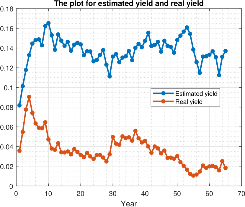
(a) Yield

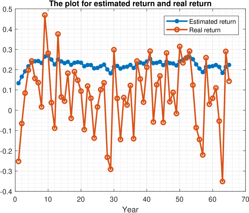
(b) Return

Figure 1.1: Kalman Filter Results for Yield and Real Return

The results are showing that kalman filter works well in first five to six years with the same trend of move and estimation value approximating to real value. After the fifth year, the value of estimations are far away from real value but keeping the same trend of move. The reason for estimation and real value deviating from fifth year is that the model is non-linear with time. The results confirm that kalman filter perfectly works on linear model and the first several steps of non-linear model, while it works worse on the later part of non-linear model. Thus, the use of extended Kalman filter– Unscented Kalman filter, is needed to solve this non-linear problem.

Chapter 2 Unscented Filtering and Nonlinear Estimation

The extended Kalman Filter (EKF) has been widely used to deal with non-linear problem. However, it is hard to implement and the results are often inaccurate. the Unscented transformation (UT) has been developed as an improvement to utilize information of mean and covariance to accurate results and make it easier to implement. The method is to select sigma points according to their mean $\mu_{x}$ and covariance $\sigma_{x}$ (i.e. choosing data in range of $[-2\sigma_{x},2\sigma_{x}]$). The non-linear function is applied to each point to generate a cloud of points. Then transformed mean and covariance can be obtained from calculating mean and variance of those sigma points. There are two advantages of using UT transformation. The first is selected sigma points are no longer randomly chosen but containing information of an unknown distribution, which is sufficient to operate statistic computation. Furthermore, mean and covariance are linearly transformable (i.e. mean $\bar{x}$ will be $T\bar{x}$ after operating transformation T, and covariance $\Sigma_{x}$ will be $T\Sigma_{x}T^{T}$) The second is weights for sigma points can be adjusted in ways such that more points around mean can be captured.

2.0.1 General Algorithms for Unscented Kalman Filter

1) Generating sigma points:
Consider a set of sigma points S with given mean and covariance, it contains $(2N_{x}+1)$ vectors and their associate weights $S=\{i=0,1,...2N_{x}:X^{(i)},W^{(i)}\}$. By convention, $W^{(0)}$ will be the weight on the mean point, which is indexed as the zeroth point

$$X^{(0)}=\bar{X}$$

$$W^{(0)}=W^{(0)}$$

The other $2N-x$ points lie on the $\sqrt{N_{x}}$th covariance with half points on the left side of mean and half on the right side of mean

$$X^{(i)}=\bar{X}+\big{(}\sqrt{\frac{N_{x}}{1-W^{(0)}}\Sigma_{x}}\big{)}_{i}$$

$$W^{(i)}=\frac{1-W^{(0)}}{2N_{x}}$$

$$X^{(i+N_{x})}=\bar{X}-\big{(}\sqrt{\frac{N_{x}}{1-W^{(0)}}\Sigma_{x}}\big{)}_{i}$$

$$W^{(i+N_{x})}=\frac{1-W^{(0)}}{2N_{x}}$$

2) Generating transformed set, which is normally the expectation value through Plant model

$$\hat{X}_{n}^{(i)}=f[X_{n}^{(i)},\mu_{n}].$$

3) Computing predicted mean

$$\hat{\mu}_{n}=\sum_{i=0}^{p}W^{(i)}\hat{X}_{n}^{(i)}.$$

4) And computing predicted covariance

$$\hat{K}_{n}=\sum_{i=0}^{p}\{\hat{X}_{n}^{(i)}-\hat{\mu}_{n}\}\{\hat{X}_{n}^{(i)}-\hat{\mu}_{n}\}^{T}.$$

5) Plugging each of the predicted points to observation model

$$\hat{Y}_{n}^{(i)}=g[X_{n}^{(i)}].$$

6) Computing observation mean

$$\hat{Y}_{n}=\sum_{i=0}^{p}W^{(i)}\hat{Y}_{n}^{(i)}.$$

7) And computing observation covariance

$$\hat{S}_{n}=\sum_{i=0}^{p}\{\hat{Y}_{n}^{(i)}-\hat{Y}_{n}\}\{\hat{Y}_{n}^{(i)}-\hat{Y}_{n}\}^{T}.$$

8) Finally updating normal Kalman Filter Equations

$$\mathcal{V}_{n}=Y_{n}-\hat{Y}_{n}$$

$$W_{n}=\hat{K}_{n}\hat{Y}_{n}^{-1}$$

$$\mu_{n}=\hat{\mu}_{n}+W_{n}\mathcal{V}_{n}$$

$$K_{n}=\hat{K}_{n}-W_{n}\hat{S}_{n}W_{n}^{T}$$

2.0.2 Implementation for Yield and Real Return Model

Here we use the same example of yield and real return model. Expected results are better by implementing Unscented Kalman filter. That is

$$Z_{n}=\Phi_{n-1}Z_{n-1}+D+\sqrt{X_{n-1}}CW_{n}$$ (1.10)

$$Y_{n}=H_{n}Z_{n}+VB_{n}$$ (1.11)

In order to generate sigma points, $W^{(0)}=\frac{1}{3}$ and $2N_{x}=400$ have been set. With initial mean of sigma points $\mu_{n}=H_{n}^{-1}(Y_{n}-VB_{n})$ and initial covariance as zero matrix, one can repeat the algorithms by using steps listed. Each time by choosing factorization of $\hat{K}_{n}$, we can get the covariance of sigma points. When implementing the algorithm, we changed a little bit in step 2. Instead of using expectation, we use the whole function to process sigma particles because the value of noisy parameters are relatively high and it will be better to mimic points adding those noise. Each time we need to guarantee $X_{n}$ is positive.

2.0.3 Results for Yield and Real Return Model

Predicted dividend yield matches highly with the real yield from the figure, which means the prediction for yield is pretty sucess. Predicted real return does not match with the real return well but keep the same trend. Reasons for diiference of the results are: First, variance for real return is higher than yield which enlarge the error for mis-allocated sigma points. Sigma points for yield are intensive since it has relatively stable trend with lower variance. Second, for updating each step, real return highly depends on the prediction of yield from previous step, so the predicted error for yield can be exaggerated further.

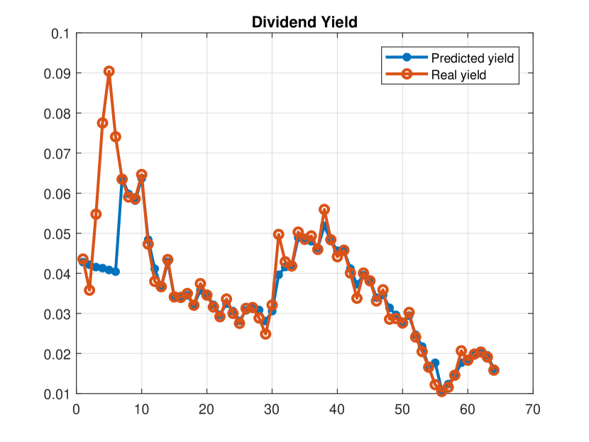
(a) Yield

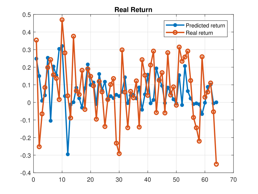
(b) Return

Figure 2.1: Unscented Filter Results for Yield and Real Return

Chapter 3 Particle Flow Filter

Particle Filters have the problem of particle degeneracy caused by Bayesian Rule, especially in dealing with high dimensional state vectors. The algorithm puts particles to wrong places when multiplying prior function with likelihood function. Particle Flow Filter is derived to improve the estimation accuracy in high-dimensional space by involving move functions of particles and it is significantly mitigate the problem of degeneracy. We set each particle in d-dimensional space as a function of $\lambda$ denoting as $x(\lambda)$, in which lambda is continuously changing like time. $\lambda$ starts from 0 and ends up with 1 giving the results of moving from points to next points.

3.0.1 Generalized Gromov Method for stochastic Particle Flow Filters

We start from constructing the stochastic differential equation for flow of particles:

$$dx=f(x,\lambda)d\lambda+Q(x)^{\frac{1}{2}}dW_{\lambda}$$ (3.0.1)

Here $f(x,\lambda)$ is the moving function for particles and Q is the covariance matrix of the diffusion $W_{\lambda}$. $W_{\lambda}$ is the measurement noise generated according to $\lambda$.
In order to get the solution of $f(x,\lambda)$ and Q(x), probability density function $log\ P(x,\lambda)$ is essential to be introduced. We have:

$$\log\ P(x,\lambda)=\log\ g(x)+\lambda\log\ h(x)-\log\ K(\lambda)$$ (3.0.2)

The generalized probability density function has the form of :

$$p(x,\lambda)=\frac{g(x)h(x)^{\lambda}}{\int_{\mathbb{R}^{d}}g(x)h(x)^{\lambda}\,dx}=\frac{g(x)h(x)^{\lambda}}{K(\lambda)},$$ (3.0.3)

in which h(x) is the likelihood, g(x) is from part a and $K(\lambda)$ is the norm of product of $g(x)andh(x)^{\lambda}$. The purpose of $K(\lambda)$ is to normalize the conditional probability density.
By using equation (3.0.2), one can solve $f(x,\lambda)$ by setting specific $Q(x)$ to simplify the PDE for f. The PDE has the form of :

$$\frac{\partial{\log h}}{\partial x}=-f^{T}\frac{\partial^{2}\log\ P}{\partial x^{2}}-\frac{\partial div(f)}{\partial x}-\frac{\partial\log P}{\partial x}\frac{\partial f}{\partial x}+\frac{\partial[div(Q\frac{\partial P}{\partial x})/2P]}{\partial x}$$ (3.0.4)

The simplest way is to set:

$$-\frac{\partial div(f)}{\partial x}-\frac{\partial logP}{\partial x}\frac{\partial f}{\partial x}+\frac{\partial[div(Q\frac{\partial P}{\partial x})/2P]}{\partial x}=0$$ (3.0.5)

Then the solution for $f(x,\lambda)$ is :

$$f(x,\lambda)=-[\frac{\partial^{2}\log P(x,\lambda)}{\partial x^{2}}]^{-1}(\frac{\partial\log h(x)}{\partial x})^{T}$$ (3.0.6)

According to equation (3.0.5), the corresponding covariance function Q is:

$$Q=[P-\lambda PH^{T}(R+\lambda HPH^{T})^{-1}HP]H^{T}R^{-1}H[P-\lambda PH^{T}(R+\lambda HPH^{T})^{-1}HP]$$ (3.0.7)

where $R$ is the measurement noise covariance matrix, $P$ is the prior covariance matrix, and $H$ is the sensitive matrix in measurement model.
In order to keep the solution of $Q$ from equation (3.0.7) as symmetric matrix, one can implement the following method to symmetry Q immediately:

$$Q=\frac{Q+Q^{T}}{2}$$ (3.0.8)

Algorithm 3.0.1.

(Algorithm for implementing Particle Flow Filter with diffusion)

• a. Use Monte Carlo method randomly choose $N$ particles around observation, and generate particle density function $g(x)$ as prior density function.
  

• b. Choose suitable $h(x)$ as likelihood function.

• c. Compute $p(x,\lambda)$ by Equation (3.0.3), $p(x,\lambda)=\frac{g(x)h(x)^{\lambda}}{K(\lambda)}$, where $K(\lambda)=\int_{\mathbb{R}^{d}}g(x)h(x)^{\lambda}\,dx$ .

• d. Solve the moving function $f(x,\lambda)$ and measurement covariance matrix Q by equation (3.0.6) and (3.0.7). That is,

  $$f(x,\lambda)=-[\frac{\partial^{2}\log\ P(x,\lambda)}{\partial x^{2}}]^{-1}(\frac{\partial\log h(x)}{\partial x})^{T}.$$ (3.0.9)

  $$Q=[P-\lambda PH^{T}(R+\lambda HPH^{T})^{-1}HP]H^{T}R^{-1}H[P-\lambda PH^{T}(R+\lambda HPH^{T})^{-1}HP].$$

• e. Plug the value of $f(x,\lambda)$ and $Q(x)$, one can derive x by solving the PDE: $dx=f(x,\lambda)d\lambda+LdW_{\lambda}$, with L= chol(Q). We can use forward Euler scheme

  $$x^{(n+1)}=x^{(n)}+f(x^{(n)},\lambda_{n})\Delta\lambda+L\Delta W_{\lambda}$$ (3.0.10)

  or implicit Euler scheme

  $$x^{(n+1)}=x^{(n)}+f(x^{(n+1)},\lambda_{n+1})\Delta\lambda+L\Delta W_{\lambda}.$$ (3.0.11)

  f. For updating each point, repeat steps from a to e.

Remark 3.0.2.

Here $h(x)$ can be any type of distribution but we consider normal distribution with estimated mean and variance.

Remark 3.0.3.

The use of either explicit or implicit Euler method depends on the shape of $f(x,\lambda)$.

3.0.2 Implementation of Particle Flow Filter

In our previous dividend yield and S&P real return model,with the observation model as:

$$Z_{n}=\begin{pmatrix}X_{n}\\ \delta R_{n}\end{pmatrix}=\begin{pmatrix}\frac{1}{1+k}X_{n-1}+\frac{k\theta}{1+k}+\frac{\sigma}{1+k}\sqrt{X_{n-1}}\Delta W_{1,n}\\ \mu X_{n}+a\sqrt{X_{n-1}}\left(\rho\Delta W_{1,n}+\sqrt{1-\rho^{2}}\Delta W_{2,n}\right)\end{pmatrix}$$

and measurement model as:

$$Y_{n}=\begin{pmatrix}Y_{1,n}\\ Y_{2,n}\end{pmatrix}=\begin{pmatrix}X_{n}+Q_{1}B_{1,n}\\ \delta R_{n}+Q_{2}B_{2,n}\end{pmatrix}$$

We can get the particle density function is

$$g(x_{1},x_{2})=\frac{1}{2\pi\sigma_{1}\sigma_{2}\sqrt{1-\rho^{2}}}e^{-\frac{(x-\mu)^{T}\Sigma_{1}^{-1}(x-\mu)}{2}}$$

where $\mu$ is sample mean and $\Sigma_{1}$ is sample covariance

$$\Sigma_{1}=\begin{pmatrix}\sigma_{1}^{2}\ \ \rho\sigma_{1}\sigma_{2}\\ \rho\sigma_{1}\sigma_{2}\ \ \sigma_{2}^{2}\end{pmatrix}$$

We can set the likelihood function as

$$h(x_{1},x_{2})=\frac{1}{2\pi\sqrt{|\Sigma_{2}|}}e^{-\frac{(x-m)^{T}\Sigma_{2}^{-1}(x-m)}{2}}$$

where m is probability mean and $\Sigma_{2}$ is probability covariance. Conditional probability density function $P(x,\lambda)$ follows:

$$p(x,\lambda)=\frac{g(x)h(x)^{\lambda}}{||g(x)h(x)^{\lambda}||}=\frac{e^{-\frac{(x-\mu)^{T}\Sigma_{1}^{-1}(x-\mu)+\lambda(x-m)^{T}\Sigma_{2}^{-1}(x-m)}{2}}}{K(\lambda)}$$

where

$$K(\lambda)=||e^{-\frac{(x-\mu)^{T}\Sigma_{1}^{-1}(x-\mu)+\lambda(x-m)^{T}\Sigma_{2}^{-1}(x-m)}{2}}||$$

And then

$$logP(x,\lambda)=-\frac{(x-\mu)^{T}\Sigma_{1}^{-1}(x-\mu)+\lambda(x-m)^{T}\Sigma_{2}^{-1}(x-m)}{2}-log(K(\lambda))$$

$$log\ h(x)=log(\frac{1}{2\pi(\Sigma_{2})^{1/2}})-\frac{(x-m)^{T}\Sigma_{2}^{-1}(x-m)}{2}$$

$$\frac{\partial^{2}(logP(x,\lambda))}{\partial x^{2}}=-\Sigma_{1}^{-1}-\lambda\Sigma_{2}^{-1}$$

$$\frac{\partial(log\ h(x))}{\partial x}=-\Sigma_{2}^{-1}(x-m)$$

Moving function $f(x,\lambda)$ is

$$f(x,\lambda)=-[\frac{\partial^{2}log\ P(x,\lambda)}{\partial^{2}x}]^{-1}(\frac{\partial log\ h(x)}{\partial x})=-[-\Sigma_{1}^{-1}-\lambda\Sigma_{2}^{-1}]^{-1}[-\Sigma_{2}^{-1}(x-m)]$$

$$=-[\Sigma_{1}^{-1}+\lambda\Sigma_{2}^{-1}]^{-1}\Sigma_{2}^{-1}(x-m)$$

According to equation (3.0.7), the corresponding $Q(x)$ in this case is:

$$Q=[P-\lambda P(V+\lambda P)^{-1}P]V^{-1}[P-\lambda P(V+\lambda P)^{-1}P],$$

where $P$ is the prior covariance, which has the form from Kalman Filter:

$$P_{n(-)}=\Phi P_{n-1(+)}\Phi^{T}+(1\ ,\ 0)x^{(n-1)}CC^{T},$$

and $L(x)=\sqrt{Q(x)}$. Then update x with respect to $\lambda$ by Backward Euler:

$$x^{(n+1)}=x^{(n)}+f(x^{(n+1)},\lambda_{n+1})\Delta\lambda+L(x^{(n)})\Delta W_{\lambda}$$

Subtracting $m$ on each side, one can get

$$x^{(n+1)}-m=(x^{(n)}-m)-[\Sigma_{1}^{-1}+\lambda_{n+1}\Sigma_{2}^{-1}]^{-1}\Sigma_{2}^{-1}(x^{(n+1)}-m)\Delta\lambda+L(x^{(n)})\Delta W_{\lambda}.$$

Set $y^{(n+1)}=x^{(n+1)}-m$ and $y^{(n)}=x^{(n)}-m$, the equation becomes

$$y^{(n+1)}=y^{(n)}-[\Sigma_{1}^{-1}+\lambda\Sigma_{2}^{-1}]^{-1}\Sigma_{2}^{-1}y^{(n+1)}\Delta\lambda+L(x)\Delta W_{\lambda}.$$

$$(I+\Delta\lambda[\Sigma_{1}^{-1}+\lambda\Sigma_{2}^{-1}]^{-1}\Sigma_{2}^{-1})y^{(n+1)}=y^{(n)}+L(x)\Delta W_{\lambda}$$

$$y^{(n+1)}=(I+\Delta\lambda[\Sigma_{1}^{-1}+\lambda\Sigma_{2}^{-1}]^{-1}\Sigma_{2}^{-1})^{-1}(y^{(n)}+L(x)\Delta W_{\lambda})$$

$$x^{(n+1)}=(I+\Delta\lambda[\Sigma_{1}^{-1}+\lambda\Sigma_{2}^{-1}]^{-1}\Sigma_{2}^{-1})^{-1}(x^{(n)}-m+L(x)\Delta W_{\lambda})+m$$

3.0.3 Results for yield and real return model

By involving function of movement $f(x,\lambda)$, accuracy for predicting of real return has been highly increased. The validity of using particle flow methods has been proved. The trends for predicted yield are highly similar to the real trend. And prediction for yield has great performance at the years with large fluctuation but cannot mimic the value with lower fluctuation. That is because we set relative larger covariance for likelihood matrix, which means it cannot do better when the real covariance become lower. Then the corresponding cons for Particle Flow Filter is clear to see that constant likelihood function $h(x)$ is hard to satisfy the change for each points.

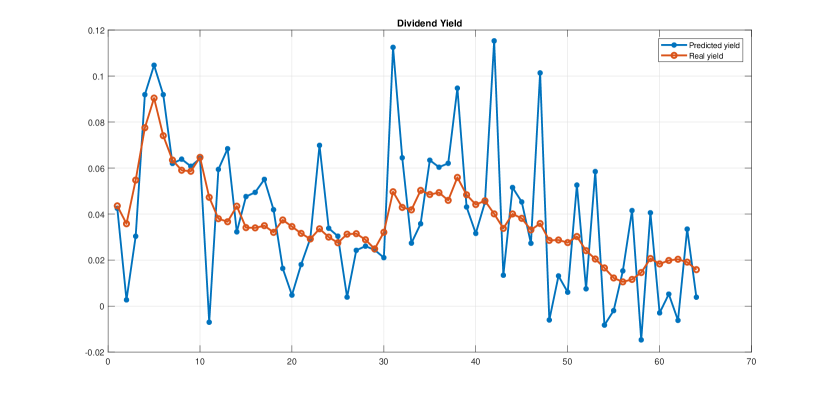
(a) Yield

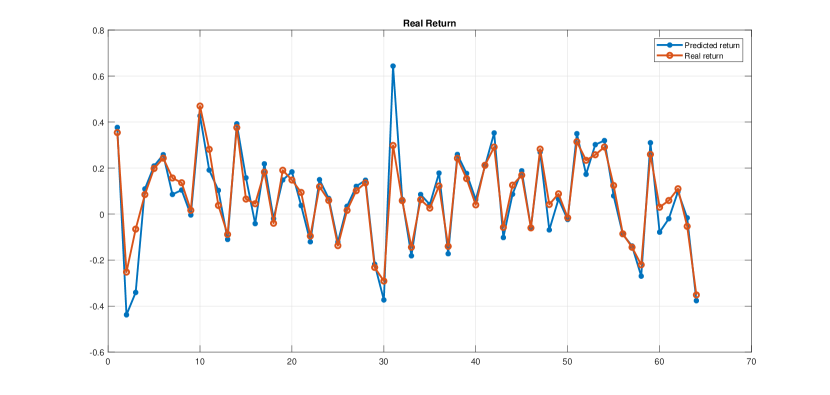
(b) Return

Figure 3.1: Particle Flow Filter Results for Yield and Real Return

Bibliography

- [1] Narayan Kovvali ; Mahesh Banavar ; Andreas Spanias. An Introduction to Kalman Filtering with MATLAB Examples. Morgan & Claypool, Reading, 9781627051408, 2013.
- [2] Simon J. Julier ; Jeffery K. Uhlmann. Unscented Filtering and Nonlinear estimation. Digital Objective Identifier, 0018-9219/04, 2014.
- [3] Fred Daum ; Jim Huang ; Arjang Noushin Generalized Gromov method for Stochastic Particle Flow Filters 0277-786X/17, 2017