A connection between Living Liquid Crystals and electrokinetic phenomena in nematic fluids
	Christopher Conklin1, Jorge Viñals2, and Oriol T. Valls3
	We develop a formal analogy between configurational stresses in two distinct physical systems, and study the flows that they induce when the configurations of interest include topological defects. The two systems in question are electrokinetic flows in a nematic fluid under an applied electrostatic field, and the motion of self propelling or active particles in a nematic matrix (a living liquid crystal). The mapping allows the extension, within certain limits, of existing results on transport in electrokinetic systems to self propelled transport. We study motion induced by a pair of point defects in a dipole configuration, and steady rotating flows due to a swirling vortex nematic director pattern. The connection presented allows the design of electrokinetic experiments that correspond to particular active matter configurations that may, however, be easier to conduct and control in the laboratory.

1 Introduction

Research on electrokinetic phenomena in liquid crystal nematics is currently addressing the use of electrostatic fields to induce fluid flow, and to control the motion of suspended particles. The anisotropic physical properties of the liquid crystal molecules together with long range orientational order in a nematic phase enable complex streaming flows in the bulk that can be controlled by manipulating either the nematic director or applied electric fields. Similarly, suspending self propelling particles (“active matter”) in a nematic matrix has been shown to allow control and steering of their motion by designing appropriate nematic director configurations. In this paper, we advance a formal analogy between these two distinct physical systems that allows the extension, within certain limits, of results on transport in electrokinetic systems to those for self propelled objects. Such a connection may allow the design of electrokinetic experiments that are analogs of particular active matter configurations of interest, and hence easier to conduct and control in the laboratory.

The term electrokinetic phenomena refers collectively to induced response in fluid electrolytes under imposed electrostatic fields, and to any resulting fluid flow or suspended particle motion. Microscale manipulation of colloidal particles and fluids by electric fields is a broad area of active scientific research ranging from fundamental studies of non-equilibrium phenomena ^{1, 2, 3, 4} to the development of practical devices for informational displays, portable diagnostics, sensing, delivery, and cell sorting ^{5, 6, 7}. Electrokinetic fluid transport is important in a variety of engineering, soft matter, and biological systems. For example, electrokinetic flows have been used to create “lab on a chip” micropumps, nanofluidic diodes, microfluidic field effect transistors, and e-ink devices such as book readers^{8, 9, 10, 11}. Our specific focus is on electrokinetic phenomena in the particular case in which the fluid is a liquid crystal in the nematic phase. Although ionic impurities are always present in liquid crystal media, their effect has been usually considered as parasitic, and thus to be minimized in applications. However, the recent discovery of electrokinetic phenomena in nematic suspensions ¹² has opened a variety of avenues for the creation and control of designer flows that rely on the anisotropy of the medium ¹³.

We explore here the mapping between the electrokinetic problem just outlined, and that of the motion of self propelled particles in a nematic matrix. In the latter case, the suspended particles are endowed with an assumed speed (of internal origin) along a preferred direction. When such particles are immersed in a nematic matrix (a “living liquid crystal”), they affect, and are affected by, the orientational order in the matrix. Particles move preferentially along the nematic direction in the matrix, both because of their intrinsic velocity, and because of forces of elastic origin imparted by the nematic medium. This motion of active particles drives flow in living liquid crystals with a body force $\bm{f}\sim\nabla\cdot(c\bm{nn})$, where $c$ is the concentration of active particles and $\bm{n}$ is the nematic director ¹⁴. We show that under certain conditions it is possible to map this physical problem to the electrokinetic problem discussed above, and hence to use existing results concerning flow induced by nematic director patterns to the case of living liquid crystals. We develop this correspondence below, and study specific configurations of interest in which the motion of active particles can be controlled by imposed nematic director distributions. The active matter experiments of interest consist of a thin film of bacteria (such as Bacillus subtilis) suspended in a lyotropic chromonic liquid crystal matrix ^{15, 16}. Our modeling is confined to two dimensions. The experiments that we focus on, both in living liquid crystals and electrokinetic flows ¹⁷, have been conducted in thin cells with patterned, fixed, director orientations. There is no indication in the experiments of any flow structure along the thin dimension, although the existence of no slip conditions on both top and bottom cell surfaces may introduce significant flow damping. For flows driven by director configurations involving isolated defects, damping may be important relative to viscous Newtonian stresses only at distances from the cores much larger than the cell thickness. In the case of Living Liquid Crystal experiments, the cell thickness is on the order of $5\mu$m, yet the swirling bacteria ensemble has its largest velocity around 35 $\mu$m. On the other hand, cell ticknesses in electrokinetic experiments are much larger, on the order of 50-100 $\mu$m ¹⁷. In order to highlight functional dependencies of flow velocities with distance away from defects, and to compare our results with existing experiments and models, we confine our analysis below to two dimensions, and neglect viscous damping terms. However, it is straightforward to include them in the analysis as they are linear in the velocity. Finally, note that although we consider a two-dimensional problem, all densities introduced are defined per unit volume.

2 Liquid crystal electrokinetics in an oscillatory electric field

2.1 Governing equations for the ionic system

We consider a thin film of a liquid crystalline fluid, electrically neutral, in its nematic phase. The fluid contains two ionic species of charge $\pm e$, where $e$ is the elementary (positive) charge. It is subjected to an external electrostatic field, spatially uniform but oscillatory in time, $\bm{E}_{0}$. The equations governing the evolution of the system include species mass conservation, momentum conservation in the fluid, electrostatic equilibrium, and torque balance on the liquid crystal molecules ¹⁸. Species mass conservation reads,

$$\frac{\partial c_{k}}{\partial t}+\nabla\cdot(\bm{v}c_{k})=\nabla\cdot\left(\bm{D}\cdot\nabla c_{k}-c_{k}z_{k}\bm{\mu}\cdot\bm{E}\right),$$ (1)

where $c_{k},k=1,2$ is the concentration of species $k$, $z_{1}=1,z_{2}=-1$, $\bm{v}$ is the barycentric velocity, which is equal to that of the liquid crystal as the masses of the ions are negligible. The quantities $\bm{D}$ and $\bm{\mu}$ are the mass diffusivity and ionic mobility tensors respectively, which will be assumed to be anisotropic and depend on the local orientation of the liquid crystalline molecule. They are also assumed to obey Einstein’s relation $\bm{D}=({k_{B}T}/{e})\bm{\mu}$. The mobility tensor $\bm{\mu}$ is also assumed to be anisotropic, and to depend on the local orientation of the nematic ¹⁹ via $\mu_{ij}=\mu_{\perp}\delta_{ij}+\Delta\mu\;n_{i}n_{j}$, where $\delta_{ij}$ is the Kroenecker delta, and we define $\Delta\mu=\mu_{\parallel}-\mu_{\perp}$, where $\mu_{\parallel}$ and $\mu_{\perp}$ are the ionic mobilities parallel and perpendicular to $\bm{n}$, respectively. There is a great variety of possible electrokinetic effects in a nematic suspension depending on physical parameters and frequency of the applied fields. We focus on parameter ranges suitable for experiments in electroosmotic flow and electrophoretic motion as given, for example, in Peng, et al. ¹⁷. In particular, we will focus on the limit of small anisotropy $\Delta\mu/\mu_{\perp}\ll 1$ ($\Delta\mu/\mu_{\perp}\approx 0.4$ in typical experiments ¹⁷).

In the low frequency range of interest in electrokinetic experiments, the system is assumed to be in electrostatic equilibrium, so that the total electrostatic field in the medium satisfies

$$\epsilon_{0}\nabla\cdot(\bm{\epsilon}\cdot\bm{E})=\rho$$ (2)

with charge density $\rho=e(c_{1}-c_{2})$. Although the liquid crystal molecules are not charged, they are polarizable ²⁰. The nematic is assumed to be a linear dielectric medium, with dielectric tensor $\epsilon_{ij}=\epsilon_{\perp}\delta_{ij}+\Delta\epsilon\;n_{i}n_{j}$, with $\Delta\epsilon=\epsilon_{\parallel}-\epsilon_{\perp}$, where $\epsilon_{\parallel}$ and $\epsilon_{\perp}$ are the dielectric constants parallel and perpendicular to $\bm{n}$, respectively.

The liquid crystal is incompressible, $\nabla\cdot\bm{v}=0$, and flow is overdamped (typical Reynolds number $Re\sim 10^{-5}-10^{-4}$). Momentum balance then reduces to the balance between the incompressible viscous stresses and the body forces exerted by the ionic species and the nematic polarization in a field^{21, 22},

$$\nabla\cdot\bm{T}+\rho\bm{E}+(\bm{D^{\prime}}\cdot\nabla)\bm{E}=0,$$ (3)

where $D^{\prime}_{i}=\epsilon_{0}\epsilon_{ij}E_{j}$ is the electric displacement field. The stress tensor is $T_{ij}=-p\delta_{ij}+T_{ij}^{e}+\tilde{T}_{ij}$, where $p$ is the hydrostatic pressure and $\bm{T^{e}}$ is the elastic stress,

$$T_{ij}^{e}=-\frac{\partial f}{\partial(\partial_{j}n_{k})}\frac{\partial n_{k}}{\partial x_{i}}$$ (4)

with $f$ denoting the Oseen-Frank elastic free energy density ²⁰. The viscous stress, $\bm{\tilde{T}}$, is assumed to be given by the Leslie-Ericksen model ²⁰. The last term on the left hand side of Eq. (3) can be written as,

$$(\bm{D^{\prime}}\cdot\nabla)\bm{E}=\nabla\left(\frac{1}{2}\epsilon_{0}\epsilon_{\perp}|\bm{E}|^{2}\right)+\epsilon_{0}\Delta\epsilon(\bm{n}\cdot\bm{E})(\bm{n}\cdot\nabla)\bm{E}.$$ (5)

The first term in Eq. (5) contributes only to a change in pressure and does not affect the flow velocity. Thus with a redefinition of the pressure, Eq. (3) can be rewritten as,

$$\nabla\cdot\bm{T}+\rho\bm{E}+\epsilon_{0}\Delta\epsilon(\bm{n}\cdot\bm{E})(\bm{n}\cdot\nabla)\bm{E}=0.$$ (6)

Eq. (2) implies the charge density is linear in the electric field¹⁸; thus both driving terms in Eq. (6) are quadratic in the electric field ²², leading to persistent flow even in an AC field.

Angular momentum conservation defines the dynamics of the director. A torque balance argument yields ²⁰

$$\bm{n}\times\bm{h^{0}}-\bm{n}\times\bm{h}^{\prime}+\epsilon_{0}\Delta\epsilon(\bm{n}\cdot\bm{E})(\bm{n}\times\bm{E})=0,$$ (7)

where

$$h^{0}_{i}=-\frac{\partial f}{\partial n_{i}}+\frac{\partial}{\partial x_{j}}\frac{\partial f}{\partial(\partial_{j}n_{i})},\quad\quad h^{\prime}_{i}=\gamma_{1}N_{i}+\gamma_{2}A_{ij}n_{j},$$ (8)

with $\gamma_{1}$ and $\gamma_{2}$ being rotational viscosities, $N_{i}=\dot{n}_{i}-W_{ij}n_{j}$, and $A_{ij}=\frac{1}{2}\left(\frac{\partial v_{j}}{\partial x_{i}}+\frac{\partial v_{i}}{\partial x_{j}}\right)$ and $W_{ij}=\frac{1}{2}\left(\frac{\partial v_{i}}{\partial x_{j}}-\frac{\partial v_{j}}{\partial x_{i}}\right)$ the symmetric and antisymmetric parts of the velocity gradient tensor. The first term in Eq. (7) corresponds to the elastic torque on the director field, the second term corresponds to viscous torque, and the third term is the torque due to the anisotropy of nematic polarization.

2.2 Variable orientation electric field as the analog of active stress

We consider an imposed electric field that contains two orthogonal components of different frequency and phase, $\bm{E}_{0}=E_{x}\bm{\hat{x}}\cos(\omega_{x}t)+E_{y}\bm{\hat{y}}\cos(\omega_{y}t+\psi)$. This field reduces to a rotating field of constant magnitude when $E_{x}=E_{y}$, $\omega_{x}=\omega_{y}$, and $\psi=\pi/2$. We introduce dimensionless variables as follows: We scale the electric field by $E_{x}$ and time by $\omega_{x}^{-1}$; thus in dimensionless units, the applied field is $\bm{E}_{0}=\bm{\hat{x}}\cos t+A\bm{\hat{y}}\cos(\beta t+\psi)$, where $A=E_{y}/E_{x}$ and $\beta=\omega_{y}/\omega_{x}$. We scale spatial variables by system size $L$, and the total ionic concentration $C=c_{1}+c_{2}$ by its average $c_{0}$. The scale of the charge density is ¹⁸ $\epsilon_{0}\epsilon_{\perp}E_{x}/L$, while the scale of the flow velocity and pressure are ¹⁸ $\epsilon_{0}\epsilon_{\perp}E_{x}^{2}L/\alpha_{4}$ and $\epsilon_{0}\epsilon_{\perp}E_{x}^{2}$. The resulting set of dimensionless equations are,

$$\Omega\frac{\partial C}{\partial t}+U\frac{\partial(Cv_{i})}{\partial x_{i}}=\gamma\frac{\partial}{\partial x_{i}}\left[\frac{D_{ij}}{D_{\perp}}\frac{\partial C}{\partial x_{j}}\right]-Y^{2}\frac{\partial}{\partial x_{i}}\left[\rho\frac{\mu_{ij}}{\mu_{\perp}}E_{j}\right]$$ (9)

$$\Omega\frac{\partial\rho}{\partial t}+U\frac{\partial(\rho v_{i})}{\partial x_{i}}=\gamma\frac{\partial}{\partial x_{i}}\left[\frac{D_{ij}}{D_{\perp}}\frac{\partial\rho}{\partial x_{j}}\right]-\frac{\partial}{\partial x_{i}}\left[C\frac{\mu_{ij}}{\mu_{\perp}}E_{j}\right]$$ (10)

$$\frac{\partial}{\partial x_{i}}\left[\frac{\epsilon_{ij}}{\epsilon_{\perp}}E_{j}\right]=\rho,$$ (11)

$$\nabla\cdot\bm{T}+\rho\bm{E}+\frac{\Delta\epsilon}{\epsilon_{\perp}}(\bm{n}\cdot\bm{E})(\bm{n}\cdot\nabla)\bm{E}=0,\quad\quad\bm{T}=-p\mathbb{I}+\frac{1}{\text{Er}}\bm{T}^{e}+\bm{\tilde{T}},$$ (12)

$$\bm{n}\times\bm{h}^{0}-\text{Er}\left(\bm{n}\times\bm{h^{\prime}}-\frac{\Delta\epsilon}{\epsilon_{\perp}}(\bm{n}\cdot\bm{E})(\bm{n}\times\bm{E})\right)=0,$$ (13)

where $\Omega=\omega_{x}\tau_{\rho}$ is the driving frequency relative to the charging time $\tau_{\rho}=\epsilon_{0}\epsilon_{\perp}/(ec_{0}\mu_{\perp})$, $U=\tau_{\rho}\epsilon_{0}\epsilon_{\perp}E_{x}^{2}/\alpha_{4}$, $\gamma=\tau_{\rho}D_{\perp}/L^{2}$, where $D_{\perp}$ is the ionic diffusivity perpendicular to $\bm{n}$, $Y=\epsilon_{0}\epsilon_{\perp}E_{x}/(Lec_{0})$, and $\text{Er}=\epsilon_{0}\epsilon_{\perp}E_{x}^{2}L^{2}/K$ is the Ericksen number, the ratio of viscous to elastic torques, with $K$ as the average value of the elastic constants in the Oseen-Frank elastic free energy. Note that $\gamma$ can be also be written as $\gamma=\lambda_{D}^{2}/L^{2}$, where $\lambda_{D}=\sqrt{\epsilon_{0}\epsilon_{\perp}k_{B}T/(e^{2}c_{0})}$ is the Debye length. Also, in the scaled variables $N_{i}=(\Omega/U)\partial_{t}n_{i}+v_{j}\partial_{j}n_{i}-W_{ij}n_{j}$. Eqs. (9) - (13) represent the full set of governing equations in dimensionless form.

Consistent with typical electrokinetic experiments, we assume that fluid anisotropy is small, and we expand the governing equations in powers of $\Delta\mu/\mu_{\perp}$ and $\Delta\epsilon/\epsilon_{\perp}$. At zeroth order in these two quantitites, the equations correspond to a purely isotropic medium, with $C^{(0)}=1$, $\rho^{(0)}=0$, $\bm{v}^{(0)}=0$, and $\bm{E}^{(0)}=\bm{E}_{0}$. Using Eq. (11), Eqs. (9) and (10) at first order can be written as,

$$\Omega\frac{\partial C^{(1)}}{\partial t}=\gamma\nabla^{2}C^{(1)}-Y^{2}(\bm{E}_{0}\cdot\nabla)\rho^{(1)}$$ (14)

$$\Omega\frac{\partial\rho^{(1)}}{\partial t}=\gamma\nabla^{2}\rho^{(1)}-\rho^{(1)}+\left(\frac{\Delta\epsilon}{\epsilon_{\perp}}-\frac{\Delta\mu}{\mu_{\perp}}\right)\nabla\cdot(\bm{n}(\bm{n}\cdot\bm{E}_{0}))-(\bm{E}_{0}\cdot\nabla)C^{(1)}.$$ (15)

Similarly, we assume a system in which $Y^{2}/(4\gamma\sqrt{1+\Omega^{2}})\ll 1$, which can be shown implies $C^{(1)}$ and $\rho^{(1)}$ decouple ¹⁸. Furthermore, since the Debye length in electrokinetic systems is typically on the order of $\lambda_{D}\sim 10^{-6}$ m, while cell sizes are $L\sim 10^{-4}$ to $10^{-3}$ m, we find $\gamma\sim 10^{-6}$ to $10^{-4}$. Thus the diffusion term in Eq. (15) is negligible far from nematic defect cores¹⁸. Therefore Eq. (10) can be written to first order in the anisotropies as,

$$\Omega\frac{\partial\rho}{\partial t}+\rho=\left(\frac{\Delta\epsilon}{\epsilon_{\perp}}-\frac{\Delta\mu}{\mu_{\perp}}\right)\nabla\cdot(\bm{n}(\bm{n}\cdot\bm{E}_{0})).$$ (16)

The solution to Eq. (16) is given by,

$$\rho(\bm{r},t)=\left(\frac{\Delta\epsilon}{\epsilon_{\perp}}-\frac{\Delta\mu}{\mu_{\perp}}\right)\frac{\cos(t-\delta)}{\sqrt{1+\Omega^{2}}}\nabla\cdot(\bm{n}n_{x})+\left(\frac{\Delta\epsilon}{\epsilon_{\perp}}-\frac{\Delta\mu}{\mu_{\perp}}\right)\frac{\cos(\beta t+\psi-\delta_{2})}{\sqrt{1+(\beta\Omega)^{2}}}A\nabla\cdot(\bm{n}n_{y}),$$ (17)

with $\tan\delta=\Omega$ and $\tan\delta_{2}=\beta\Omega$.

Since the applied field $\bm{E}_{0}$ is spatially uniform, the body force on the fluid due to nematic polarization (the last term on the left hand side of Eq. (12)) is second order in the anisotropies. To first order in $\Delta$, the body force on the nematic fluid is therefore $\bm{f}\approx\rho\bm{E}_{0}=\rho(\bm{r},t)(\bm{\hat{x}}\cos t+A\bm{\hat{y}}\cos(\beta t+\psi))$, or

$$\bm{f} = \left(\frac{\Delta\epsilon}{\epsilon_{\perp}}-\frac{\Delta\mu}{\mu_{\perp}}\right)\left[\frac{\cos t\cos(t-\delta)}{\sqrt{1+\Omega^{2}}}\nabla\cdot(\bm{n}n_{x}\bm{\hat{x}})+\frac{A^{2}\cos(\beta t+\psi)\cos(\beta t+\psi-\delta_{2})}{\sqrt{1+(\beta\Omega)^{2}}}\nabla\cdot(\bm{n}n_{y}\bm{\hat{y}})\right.$$ (18)

$$\left.+\frac{A\cos(\beta t+\psi)\cos(t-\delta)}{\sqrt{1+\Omega^{2}}}\nabla\cdot(\bm{n}n_{x}\bm{\hat{y}})+\frac{A\cos t\cos(\beta t+\psi-\delta_{2})}{\sqrt{1+(\beta\Omega)^{2}}}\nabla\cdot(\bm{n}n_{y}\bm{\hat{x}})\right]$$

We now define a time-averaged force, $\langle\bm{f}\rangle=\lim\limits_{T\rightarrow\infty}(1/T)\int_{0}^{T}\bm{f}dt$. The time averages are performed using:

$$\lim_{T\rightarrow\infty}\frac{1}{T}\int_{0}^{T}\cos(t-\delta)\cos(\beta t+\psi)dt=\left\{\begin{array}[]{cc}\frac{1}{2}\cos(\delta+\psi),&|\beta|=1\\ 0,&\text{otherwise}\end{array}\right.$$ (19)

$$\lim_{T\rightarrow\infty}\frac{1}{T}\int_{0}^{T}\cos t\cos(\beta t+\psi-\delta_{2})dt=\left\{\begin{array}[]{cc}\frac{1}{2}\cos(\delta-\psi),&|\beta|=1\\ 0,&\text{otherwise}\end{array}\right.$$ (20)

Assume first that $|\beta|\neq 1$. Then the last two terms of Eq. (18) average to zero, and the average force is,

$$\langle\bm{f}\rangle=\left(\frac{\Delta\epsilon}{\epsilon_{\perp}}-\frac{\Delta\mu}{\mu_{\perp}}\right)\left[\frac{\nabla\cdot(\bm{n}n_{x}\bm{\hat{x}})}{2(1+\Omega^{2})}+\frac{A^{2}\nabla\cdot(\bm{n}n_{y}\bm{\hat{y}})}{2(1+(\beta\Omega)^{2})}\right]$$ (21)

For the specific choice of $A=\sqrt{(1+(\beta\Omega)^{2})/(1+\Omega^{2})}$, so that with

$$\bm{E}_{0}=\bm{\hat{x}}\cos t+\bm{\hat{y}}\sqrt{\frac{1+(\beta\Omega)^{2}}{1+\Omega^{2}}}\cos(\beta t+\psi),$$ (22)

for arbitrary $\psi$ and $\beta\neq 1$, Eq. (21) becomes,

$$\langle\bm{f}\rangle=\left(\frac{\Delta\epsilon}{\epsilon_{\perp}}-\frac{\Delta\mu}{\mu_{\perp}}\right)\frac{\nabla\cdot(\bm{n}\bm{n})}{2(1+\Omega^{2})}.$$ (23)

Equation (23) has the same form as the driving force in active nematics when the concentration of swimmers is constant ^{14, 23}. Thus our analysis predicts active-like flows on average in electrokinetic systems driven by the field of Eq. (22). If $\beta=1$, the force will not be active-like unless the director is fixed in specific configurations ²⁴.

3 Results

To illustrate features of active-like motion that would take place in the liquid crystal electrokinetic analog, we numerically investigate electrokinetic flows generated by the electric field of Eq. (22). The experimental configuration that we have in mind involves a thin film (tens of microns in thickness) of a nematic liquid crystal with tangential anchoring on top and bottom surfaces (director parallel to the surface). A photosensitive material is coated onto the plates bounding the film, which are then exposed to light that has been polarized through a mask with nanoslits etched in the desired director pattern ^{17, 25}. This exposure aligns the primary axes of photo sensitive molecules with the desired pattern ²⁶. For sufficiently thin films, the photopatterned director field is largely constant, uniform across the film. Lithographic surface patterning offers the opportunity of tailoring flow fields in nematics for specific applications, for example, to engineer flows in microfluidic channels, or to effect controlled immersed particle motion or species separation. It is also possible to design on demand director patterns which can be reconfigured dynamically during an experiment ²⁵. Such a configuration has been used recently to control the motion of bacteria in a lyotropic liquid crystal ²⁷.

The governing equations are integrated numerically with the commercial software package COMSOL. The solutions were obtained on a circular domain $C_{0}$ with radius $r_{0}=1$. Within $C_{0}$ is a second circular domain $C_{1}$ with radius $r_{1}=1/5$, in which the mesh is more finely resolved. $C_{1}$ contains 109,196 triangular elements of linear size between $6.4\times 10^{-6}$ and $1.8\times 10^{-3}$, while $C_{0}$ contains 12,790 elements with linear size between $1.6\times 10^{-4}$ and $0.13$. Additionally, $C_{0}$ contains 384 quadrilateral elements to resolve the boundary layer at $r=r_{1}$. Equations (9) through (12) are iterated in time, while the director field $\bm{n}(\bm{r})$ is held fixed. The solution is obtained with no flux boundary conditions for the concentrations, no slip boundary conditions for the velocity, and Dirichlet boundary conditions $\Phi=-x\cos(t)-yA\cos(2t)$ for the electric potential, with $A$ satisfying Eq. (22) above. The numerical solutions assume $\Delta\epsilon/\epsilon_{\perp}=0$ and $\Delta\mu/\mu_{\perp}=0.4$, consistent with recent electrokinetic experiments¹⁷. Further details of the numerical method have been discussed elsewhere ^{18, 24}. We present next the results for two director configurations which have been studied in living liquid crystal experiments: a single fixed point defect, and a pair of point defects with opposite topological charge ²⁷.

Figure 1 shows the numerically computed average velocity for the electrokinetic model when the director pattern is given by single (+1) defect of director field $\bm{n}(\bm{r})=(\cos\theta(\bm{r}),\sin\theta(\bm{r}))$ with $\theta(r,\phi)=\phi-\pi/4$ at the center of the computational domain. The angle $\phi$ is the azimuth in polar coordinates. The constant phase $-\pi/4$ creates the vortex with swirling arms studied in experiments of living liquid crystals²⁷. Interestingly, the velocity field is not parallel to the local nematic, as noted in the experiments. Whereas this is surprising in the context of a living liquid crystal in which bacteria are known to move parallel to the local director, it is not so for an electrokinetic system. In the latter case, motion is due to the local body force that originates from charge separation, and does not in general follow director lines. Instead, charge accumulates in regions in which the director is normal to the imposed electric field.

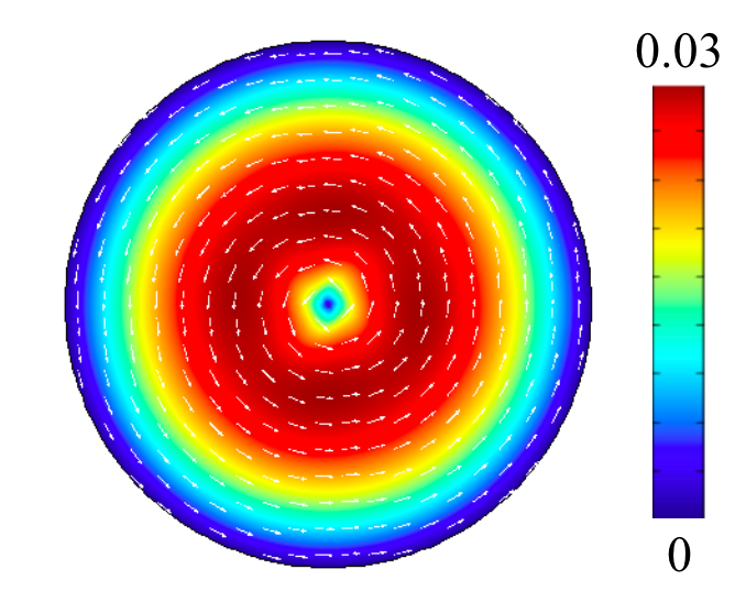
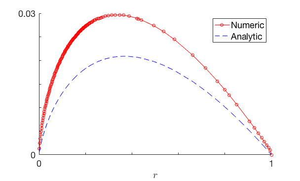
Fig.  1: Left: Average electrokinetic velocity corresponding to an imposed director field $\theta=\phi-\pi/4$, and a two frequency applied field with $\beta=2,\psi=0$, obtained by numerically integrating Eqs. (9) through (12). Right: radial velocity profile from the figure compared with the analytic solution, Eq. (29).

The velocity field obtained can be computed analytically by assuming a Newtonian fluid. Consider a director field comprising a single (+1) defect $\theta(r,\phi)=\phi+\alpha$, where $\alpha$ is an arbitrary constant phase. Equation (23) becomes,

$$\langle\bm{f}\rangle=\left(\frac{\Delta\epsilon}{\epsilon_{\perp}}-\frac{\Delta\mu}{\mu_{\perp}}\right)\frac{\cos(2\alpha)}{2r(1+\Omega^{2})}\bm{\hat{r}}+\left(\frac{\Delta\epsilon}{\epsilon_{\perp}}-\frac{\Delta\mu}{\mu_{\perp}}\right)\frac{\sin(2\alpha)}{2r(1+\Omega^{2})}\bm{\hat{\phi}}.$$ (24)

The first term in Eq. (24) may be written as $\nabla g$, where

$$g=\left(\frac{\Delta\epsilon}{\epsilon_{\perp}}-\frac{\Delta\mu}{\mu_{\perp}}\right)\frac{\log r\cos(2\alpha)}{2(1+\Omega^{2})},$$

and therefore this term can be included in the pressure field of the incompressible fluid. The second term in Eq. (24) also has a nonzero curl and can be rewritten as,

$$\left(\frac{\Delta\epsilon}{\epsilon_{\perp}}-\frac{\Delta\mu}{\mu_{\perp}}\right)\frac{\sin(2\alpha)}{2r(1+\Omega^{2})}\bm{\hat{\phi}}=\nabla\left[\left(\frac{\Delta\epsilon}{\epsilon_{\perp}}-\frac{\Delta\mu}{\mu_{\perp}}\right)\frac{\phi\sin(2\alpha)}{2(1+\Omega^{2})}\right].$$

However, if this term were included in the pressure, we would find that the pressure is not single valued, $p(\phi)\neq p(\phi+2\pi)$, which is unphysical. Therefore the body force given by the second term Eq. (24), though irrotational, cannot be included in the pressure, and must ultimately be balanced by a viscous force instead. If we assume the viscous stress to be Newtonian, $\tilde{T}_{ij}=\partial_{j}v_{i}$, an averaged momentum balance in two spatial dimensions can be written as,

$$-\nabla p^{\prime}+\nabla^{2}\bm{v}-\zeta^{2}\bm{v}+\left(\frac{\Delta\epsilon}{\epsilon_{\perp}}-\frac{\Delta\mu}{\mu_{\perp}}\right)\frac{\sin(2\alpha)}{2r(1+\Omega^{2})}\bm{\hat{\phi}}=0,\quad\nabla\cdot\bm{v}=0,$$ (25)

where

$$p^{\prime}=p-\left(\frac{\Delta\epsilon}{\epsilon_{\perp}}-\frac{\Delta\mu}{\mu_{\perp}}\right)\frac{\log r\cos(2\alpha)}{2(1+\Omega^{2})}.$$

The damping term $-\zeta^{2}\bm{v}$, $\zeta=2\sqrt{3}L/h$, arises from depth-averaging the velocity profile, assuming a Poiseuille flow in the $z$ direction ^{16, 28}. Here $h$ is the cell thickness.

The solution to Eq. (25) in a disc of dimensionless radius 1, with no-slip boundary conditions is constant $p^{\prime}$ and

$$\bm{v}=\left(\frac{\Delta\epsilon}{\epsilon_{\perp}}-\frac{\Delta\mu}{\mu_{\perp}}\right)\frac{\bm{\hat{\phi}}\sin(2\alpha)}{2\zeta(1+\Omega^{2})}\left[\frac{1}{r\zeta}-K_{1}(r\zeta)+\frac{[\zeta K_{1}(\zeta)-1]}{\zeta I_{1}(\zeta)}I_{1}(r\zeta)\right],$$ (26)

where $I_{1},K_{1}$ are modified Bessel functions of the first and second kind, respectively. When $r\zeta\gg 1$ the flow is exponentially damped. In the opposite limit,

$$\bm{v}(r\zeta\ll 1)\approx-\frac{1}{4}\left(\frac{\Delta\epsilon}{\epsilon_{\perp}}-\frac{\Delta\mu}{\mu_{\perp}}\right)\frac{\bm{\hat{\phi}}\sin(2\alpha)}{1+\Omega^{2}}[r\log r-r\eta(\zeta)],$$ (27)

where

$$\eta(\zeta)=\frac{\zeta K_{1}(\zeta)-1}{\zeta I_{1}(\zeta)}+\log\left(\frac{2}{\zeta}\right)+\frac{1}{2}-\gamma,$$

with $\gamma$ being Euler’s constant. In the special case in which $\zeta\ll 1$, $\eta(\zeta)\rightarrow 0$ and Eq. (27) reduces to,

$$\bm{v}=-\frac{1}{4}\left(\frac{\Delta\epsilon}{\epsilon_{\perp}}-\frac{\Delta\mu}{\mu_{\perp}}\right)\frac{\bm{\hat{\phi}}\sin(2\alpha)r\log r}{1+\Omega^{2}}.$$ (28)

In the specific case of $\alpha=-\pi/4$, one finds,

$$\bm{v}=\frac{1}{4}\left(\frac{\Delta\epsilon}{\epsilon_{\perp}}-\frac{\Delta\mu}{\mu_{\perp}}\right)\frac{r\ln r}{1+\Omega^{2}}\;\bm{\hat{\phi}},$$ (29)

Equation (29) is compared in Fig. 1 to a fully numerical solution of the governing equations. While there is a noticeable difference in magnitude between the two solutions, which is due to the additional approximations involved in the analytic solution, Eq. (29) (Newtonian stress, small anisotropy, etc.), both clearly exhibit an $r\log r$ dependence along $\bm{\hat{\phi}}$. This result is in agreement with the velocity profile reported by Peng, et al²⁷ for a living liquid crystal under the same fixed director configuration (Fig. 2D shows the experimentally determined azimuthal velocity profile), even though the experiments are nominally conducted in the limit $h/L\ll 1$.

We examine next a dipolar configuration comprising a (+1/2) and a (-1/2) defect pair. In the electrokinetic analog, the dipolar nature of the configuration is expected to lead to nonzero average flow, and directed from the (-1/2) defect towards the (+1/2) defect.

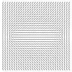
Fig.  2: Left: imposed director pattern comprising a (+1/2,-1/2) defect pair, as in the experiments of Ref. ²⁷. Center: Numerically determined fluid velocity, averaged over time. As is the case in the experiments, fluid flows from the $(-1/2)$ defect (high splay) towards the $(+1/2)$ defect (high bend) The velocity is very small near the top and bottom of the domain, leading to numerical noise in the plotting of the directional arrows. Right: central region of the velocity map magnified.

Figure 2 shows our results for the average numerical electrokinetic velocity. This flow is also in agreement with is the experiments in living liquid crystals ²⁷. In that case, it is interpreted as flow originating in regions of mixed splay-bend distortion from regions of high splay to high bend.

4 Discussion and conclusions

Despite different underlying physical mechanisms, we find that forces and corresponding flows in liquid crystal electrokinetic systems behave on average like those of living liquid crystals when the applied field has the form of Eq. (22). The driving force on an element of volume in the active system is due to the self-propulsion of bacteria along $\pm\bm{n}$ and the corresponding motion of the nematic in the opposite direction due to Newton’s Third Law ¹⁴. On the other hand, an element of volume in liquid crystal electrokinetics is driven by the electrostatic force on that element of volume. The amount and sign of charge in an element of volume is given by the anisotropy of the nematic medium. By applying a two component electric field with unequal frequencies and averaging over time, the net electrostatic force is along $\pm\bm{n}$ as well. This prediction has not yet been experimentally verified, and it remains to be seen whether higher order corrections in anisotropy and mass diffusion neglected in the analysis are indeed negligible in experimental situations.

The correspondence as derived above assumes uniform ionic and bacterial concentrations in electrokinetic and active systems, respectively. While some active nematic systems exhibit near-uniform concentration ²³, there are other cases in which variations in concentration are not negligible. In particular, the experiments of interest ¹⁵ show significant variations in bacterial concentration; the bacteria form an annulus in the swirling vortex configuration, while in the defect dipole the bacteria cluster at the (+1/2) defect and avoid the (-1/2) defect. In the electrokinetic system, one must account for the nonlinear coupling between $\rho$ and $C$ in Eqs. (9) and (10) in order to determine whether the average body force $\langle\rho\bm{E}\rangle$ is active-like when variations in $C$ are not negligible.

Additionally, charge separation induces an electric field of first order in the anisotropies, which may lead to unique flows when anisotropy is not small. Furthermore, the bacteria suspended in the nematic are typically several microns long, and thus cannot be assumed to be point particles as the ions in electrokinetic systems are. Thus, unlike ions, the bacteria in living liquid crystals are expected to distort the nematic orientation – an effect which is not captured by the electrokinetic analogy.

Finally we note a few similar features between the evolution of ionic and bacterial concentrations in the two systems. We follow the analysis of Genkin, et al.¹⁶ that introduced two concentrations $c_{\pm}$ that denote separate bacterial populations that swim with velocity $\bm{v}_{0}$ along the two possible directions parallel to the local director $\bm{n}$. Each bacterial population satisfies the equation of diffusion-advection, but can switch orientation over a reversal time scale $\tau$,

$$\frac{\partial c_{\pm}}{\partial t}+\nabla\cdot(\pm v_{0}\bm{n}c_{\pm}+\bm{v}c_{\pm})=D\nabla^{2}c_{\pm}-\frac{c_{\pm}-c_{\mp}}{\tau}.$$ (30)

On the other hand, using Poisson’s equation and assuming $\Delta\epsilon=0$, the conservation of ions in an electrokinetic system, Eq. (1), may be written as,

$$\frac{\partial c_{k}}{\partial t}+\nabla\cdot(z_{k}\Delta\mu(\bm{n}\cdot\bm{E})\bm{n}c_{k}+\bm{v}c_{k})=\nabla\cdot(\bm{D}\cdot\nabla c_{k})-\left(\frac{\mu_{\perp}ec_{k}}{\epsilon_{\perp}\epsilon_{0}}\right)z_{k}(c_{1}-c_{2})-z_{k}\mu_{\perp}(\bm{E}\cdot\nabla)c_{k}$$ (31)

The most significant physical difference between the bacterial concentrations $c_{\pm}$ and ionic concentrations $c_{k}$ is that the ionic species $c_{k}$ are physically distinct and must be conserved, while only the total bacterial concentration $c_{+}+c_{-}$ must be conserved. Nevertheless, we find a number of similarities between Eqs. (30) and (31). The anisotropy of ionic mobility leads to ionic drift along $\bm{n}$ with velocity $\Delta\mu(\bm{n}\cdot\bm{E})$, similar to bacterial self-propulsion. The ionic charging time $\epsilon_{\perp}\epsilon_{0}/(\mu_{\perp}ec_{k})$ is analogous to the bacterial reversal time $\tau$, though the charging time is a function of local concentration $c_{k}$. The last term on the right hand side of Eq. (31) is the only term without an analogous term in Eq. (30). Thus we find that the equations of bacterial concentration have a similar form to the equations of ionic concentration, though the ionic flux terms contain higher order nonlinearities than their bacterial analogs.

To summarize, we find a connection between flows in living liquid crystals and electrokinetic flows in nematics driven by a two-component oscillating field. While having different physical mechanisms, both systems drive flow with a force $\bm{f}\sim\nabla\cdot(\bm{nn})$. We compare experimental living liquid crystal flows with a fixed director pattern and numerical studies of the corresponding electrokinetic systems. While the numerical electrokinetic results show agreement with the observed bacterial flows, an experimental verification of this correspondence has not yet been performed. This mapping may be useful in using singularity solutions already known for liquid crystal electrokinetics to interpret singularity driven flows in active systems. It may also prove useful in that the experiments involving ionic systems are free of some of the complication inherent in handling active matter, including controlling the activity during the experiments. In this respect, the study of electrokinetic flows may become a tool in studying synthetic configurations involving designer flows, later to be verified directly on the living liquid crystal.

5 Conflicts of interest

There are no conflicts of interest to declare.

6 Acknowledgments

We are indebted to Oleg Lavrentovich for introducing us to the subject of Living Liquid Crystals, and for sharing experimental data. We are also indebted to Chandan Dasgupta and Peter Stoeckl for many stimulating discussions. This research has been supported by the National Science Foundation under contract DMS 1435372, by the Minnesota Supercomputing Institute, and by the Extreme Science and Engineering Discovery Environment (XSEDE) ²⁹, which is supported by National Science Foundation grant number ACI 1548562.

References

- Bazant et al. 2009 M. Z. Bazant, M. S. Kilic, B. D. Storey and A. Ajdari, Adv. Colloid Interf. Sci., 2009, 152, 48 – 88.
- Aranson 2013 I. Aranson, Physics-Uspekhi, 2013, 56, 79.
- Zöttl and Stark 2016 A. Zöttl and H. Stark, Journal of Physics: Condensed Matter, 2016, 28, 253001.
- Lavrentovich 2016 O. D. Lavrentovich, Current Opinion in Colloid and Interface Science, 2016, 21, 97–109.
- Dobnikar et al. 2013 J. Dobnikar, A. Snezhko and A. Yethiraj, Soft Matter, 2013, 9, 3693.
- Ramos 2011 A. Ramos, Electrokinetics and Electrohydrodynamics in Microsystems, Springer-Verlag, Wien, 2011.
- Bazant and Squires 2010 M. Bazant and T. Squires, Current Opinion in Colloid and Interface Science, 2010, 15, 203.
- Studer et al. 2004 V. Studer, A. Pépin, Y. Chen and A. Ajdari, The Analyst, 2004, 129, 944–949.
- Zhao and Yang 2012 C. Zhao and C. Yang, Microfluid Nanofluid, 2012, 13, 179–203.
- Comiskey et al. 1998 B. Comiskey, J. D. Albert, H. Yoshizawa and J. Jacobson, Nature, 1998, 394, 253–255.
- Klein 2013 S. Klein, Liquid Crystals Reviews, 2013, 1, 52–64.
- Lazo et al. 2014 I. Lazo, C. Peng, J. Xiang, S. Shiyanovskii and O. Lavrentovich, Nature Comm., 2014, 5, 5033.
- Hernández Navarro et al. 2014 S. Hernández Navarro, P. Tierno, J. Farrera, J. Ignés Mullol and F. Sagués, Angewandte Chemie-International Edition, 2014, 53, 10696–106700.
- Aditi Simha and Ramaswamy 2002 R. Aditi Simha and S. Ramaswamy, Phys. Rev. Lett., 2002, 89, 058101.
- Peng et al. 2016 C. Peng, T. Turiv, Y. Guo, Q.-H. Wei and O. D. Lavrentovich, Science, 2016, 354, 882–885.
- Genkin et al. 2017 M. M. Genkin, A. Sokolov, O. D. Lavrentovich and I. S. Aranson, Phys. Rev. X, 2017, 7, 11029.
- Peng et al. 2015 C. Peng, Y. Guo, C. Conklin, J. Viñals, S. Shiyanovskii, Q.-H. Wei and O. D. Lavrentovich, Phys. Rev. E, 2015, 92, 052502.
- Conklin and Viñals 2017 C. Conklin and J. Viñals, Soft Matter, 2017, 13, 725–739.
- Helfrich 1969 W. Helfrich, J. Chem. Phys., 1969, 51, 4092.
- de Gennes and Prost 1993 P. de Gennes and J. Prost, The Physics of Liquid Crystals, Clarendon, Oxford, 1993.
- de Groot and Mazur 1984 S. de Groot and P. Mazur, Non-equilibrium Thermodynamics, Dover, New York, 1984.
- Tovkach et al. 2016 O. Tovkach, M. Calderer, D. Golovaty, O. Lavrentovich and N. Walkington, Phys. Rev. E, 2016, 94, 012702.
- Green et al. 2016 R. Green, J. Toner and V. Vitelli, arXiv.org:1602.00561, 2016, 1–17.
- Conklin 2017 C. Conklin, Ph.D. thesis, University of Minnesota, 2017.
- Guo et al. 2016 Y. Guo, M. Jiang, C. Peng, K. Sun, O. Yaroshchuk, O. Lavrentovich and Q.-H. Wei, Advanced Materials, 2016, 28, 2353–2358.
- Yaroshchuk and Reznikov 2012 O. Yaroshchuk and Y. Reznikov, J. Mater. Chem., 2012, 22, 286–300.
- Peng et al. 2016 C. Peng, T. Turiv, Y. Guo, Q.-H. Wei and O. D. Lavrentovich, Science, 2016, 354, 882–885.
- Thom et al. 1989 W. Thom, Z. Walter and L. Kramer, Liquid Crystals, 1989, 4, 309–316.
- Towns et al. 2014 J. Towns, T. Cockerill, M. Dahan, I. Foster, K. Gaither, A. Grimshaw, V. Hazlewood, S. Lathrop, D. Lifka, G. D. Peterson, R. Roskies, J. R. Scott and N. Wilkins-Diehr, Computing in Science & Engineering, 2014, 16, 62.