Kinetic Theory of Transport Driven Current in Centrally fuelled Plasmas

Abstract

When a steady-state cylindrical plasma discharge is centrally fuelled, the collisionless radial electron flux is canonically coupled to an axial current. The identification and analysis of this transport driven current, previously reported in collisionless simulations [W. J. Nunan and J. M. Dawson, Phys. Rev. Lett. 73, 1628 (1994)], is addressed analytically and extended to the collisional regime by means of first-principles kinetic models. Collisionless radial transport is described with the standard quasilinear model and collisional velocity anisotropy relaxation with the Landau kinetic equation. When trapped particles corrections are taken into account, the solution of this kinetic model provides the analytical expression for the transport driven current in a centrally fuelled steady-state tokamak as a function of the thermonuclear power and discharge parameters. For ITER type discharges, with central fuelling, a current of about one mega-ampere is predicted by this first-principles analytical kinetic model.

I Introduction

Steady-state tokamak operation displays many practical and economical advantages Wesson and Campbell (2011); Rax (2011) and a detailed understanding of the various current generation mechanisms Fisch (2014) is needed for the successful realization of a steady-state reactor. The international ITER project in Cadarache is aimed at exploring such steady-state operation in the thermonuclear regime. Together with non-inductive current generation Fisch (1978, 1987), the bootstrap effect Bickerton, Connor, and Taylor (1971); Kadomtsev and Shafranov (1971) is expected to provide a fraction of its $15$ mega-amperes current.

Besides the bootstrap current, another self-generated current, without seed, was observed and reported Nunan and Dawson (1994); Ma and Dawson (1994) in numerical simulations when a magnetized cylindrical plasma discharge is centrally fuelled. In contributing to the toroidal current which provides the rotational transform required to cancel the vertical drift, this effect could affect plasma operation. Understanding and quantifying this effect is therefore particularly important for steady-state operation in ITER. Yet, this so-called transport driven current has received far less attention than the bootstrap current.

In this paper, we set up, solve and analyze an analytical model based on the quasilinear theory Galeev and Sagdeev (1968); Kaufman (1972) to describe turbulence-particle interactions and on the Landau collisional relaxation Robiche and Rax (2004) to describe particle-particle interactions. This first-principles model makes it possible to evaluate the expected fraction of spontaneous transport driven current in a centrally fuelled ITER type discharge when trapped particles corrections are taken into account. As it will be shown, it turns out that a non-negligible fraction of the confining current, about a mega-ampere, is expected to result from this overlooked effect.

Non-inductive current generation at a level of tens of mega-amperes is needed for a steady-state reactor Fisch (2014, 1978, 1987) and additional spontaneous toroidal currents, like the bootstrap Bickerton, Connor, and Taylor (1971); Kadomtsev and Shafranov (1971) and the effect analyzed in this paper Nunan and Dawson (1994); Ma and Dawson (1994), will improve the global power balance of a burning thermonuclear plasma.

Up to now, large tokamak discharges have been operated via edge gas puffing or pellet fuelling Wesson and Campbell (2011); Rax (2011). In comparison with edge or mid-radius fuelling, central fuelling offers conceptual advantages to peak the pressure profile and to wash out ashes and impurities which naturally accumulate near the magnetic axis. Although, it is not clear how to perform efficiently central fuelling in reactor size plasma, it is important to assess the physical consequences of central fuelling on a steady-state reactor.

The transport driven current in cylindrical or toroidal configurations is associated with the radial flux of charges in a centrally fuelled discharges. The favorable and encouraging result presented here provides a supplementary drive to develop fuelling systems able to deposit fuel very near the core of the discharge.

For a burning plasma where deuterium (D) and tritium (T) are continuously deposited near the magnetic axis, and helium ashes (He) continuously removed in the scrape of Layer (SOL) through the divertor, we estimate that the driven current is in the mega-ampere range for typical reactor size and performances. This new result is based on the following assumptions: (i) a steady-state burning D-T plasma where (ii) electron transport is due to turbulence in the quasilinear regime, (iii) current relaxation is due to electron/ion collisions, (iv) collisional transport is negligible in comparison with turbulent transport and (v) the turbulent modes are associated with rational magnetic surfaces. These five assumptions are canonical for standard tokamak models and provide a clear and realistic framework for this analytical study.

Consider a straight tokamak reactor model (a cylindrical screw pinch illustrated in Fig. 1) with a global fusion power $W_{f}$ ($\sim$ GW) . To discriminate the central fuelling effect from the bootstrap effect, or other neoclassical effects, we restrict the model to a straight tokamak with minor radius $a$, major radius $R$, safety factor $q$ and typical magnetic field $B$. The impact of trapped particles on transport driven current in tokamak is evaluated in the last section. In order to operate in steady-state, a radial flux of matter is needed from the center, where fuelling and combustion take place, toward the edge, where ashes and heat removal are operated in the SOL.

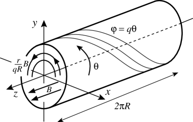
Figure 1: A straight tokamak configuration with minor radius $a$, major radius $R$ and safety factor $q$.

If neutral fuel is deposited and burned near the magnetic axis, the radial electrons flux $\Gamma_{r}$ at radius $r$ is given by

$$\Gamma_{r}=\frac{W_{f}}{4\pi^{2}rRQ_{DT}},$$ (1)

where $Q_{DT}$ is the energy yield per D/T fusion reaction ($17.6$ MeV). In this model the rate of particles central-injection/edge-extraction, $W_{f}/Q_{DT}$, corresponds to a radial ambipolar flux. However, because of their charge to mass ratio, ions are only involved through pitch-angle scattering current destruction and not through current generation. This net outward flux $\Gamma_{r}$, independent of the recycling processes Wesson and Campbell (2011); Rax (2011), is a consequence of the steady-state and central fuelling requirements and its precise nature, be it convective Ware (1970), diffusive or even non local Rax and Moreau (1989), remains an open question. A mean radial electron velocity $V$ is associated with this flux:

$$V=\frac{\Gamma_{r}}{n_{e}}\approx\frac{W_{f}}{4\pi^{2}aRQ_{DT}\left\langle n_{e}\right\rangle},$$ (2)

where $n_{e}$ is the electron density and $\left\langle n_{e}\right\rangle$ is the electron density averaged over the whole discharge volume.

Electrons transport from the core towards the SOL is expected to take place in the turbulent regime associated with a spectrum of modes. Let us consider one turbulent mode such that its local structure is periodic along the magnetic field line, with wavelength $2\pi/k_{\|}$, and periodic across the field lines, in the poloidal direction, with wavelength $2\pi/k_{\perp}$. Under the random phase approximation (RPA) Rax (2014), such a $\left(k_{\|},k_{\perp}\right)$ electrostatic, or electromagnetic, wave interacting with an electron transfers linear momentum $m_{e}\delta v_{\|}$ along the magnetic field. It also induces a displacement $\delta r$ of the guiding center radial position, which is related to this momentum transfer by

$$\Omega k_{\|}\delta r=\delta v_{\|}k_{\perp},$$ (3)

where $\Omega=eB/m_{e}$ is the cyclotron frequency, $e$ and $m_{e}$ the electron charge and mass. This effect is due to canonical momentum conservation and is put at work in alpha particles free-energy extraction Fisch and Rax (1992, 1993); Fisch and Herrmann (1994); Heikkinen and Sipil (1995); Herrmann and Fisch (1997); Ochs, Bertelli, and Fisch (2015); Cook, Dendy, and Chapman (2017) and in angular momentum injection in advanced tokamaks Rax, Gueroult, and Fisch (2017).

The linear momentum increment $m\delta v_{\|}$ given by the wave (which becomes a toroidal angular momentum in a tokamak configuration) is then dissipated through collisions, mainly through ion pitch-angle scattering, at a rate $\nu$, the pitch-angle scattering collision frequency Wesson and Campbell (2011); Rax (2011). The small transient toroidal current $\delta I$ is thus given by the expression:

$$\delta I\left(\delta r,t\right)= \frac{e}{2\pi R}\delta v_{\|}\exp\left(-\nu t\right)$$

$$= ~{}\Omega\frac{k_{\|}}{k_{\perp}}\frac{e}{2\pi R}\delta r\exp\left(-\nu t\right)\text{.}$$ (4)

We do not need the full picture of the transport process, convective, diffusive, local or non local, because we know that the sum of all the stochastic radial steps $\delta r$ is ultimately given by: $\Sigma\delta r=a$, when the center to edge transit is achieved, even with strong recycling. We also know that the average rate of radial transport $\left\langle\delta r/\delta t\right\rangle$ must be equal to $V$ in steady-state. The steady-state current $\left\langle\delta I\right\rangle$ is given by the sum of the time-averaged incremental currents created by each electron: $\left\langle\delta I\right\rangle=\int\delta Idt/\int dt$ where $\int dt=\delta r/V$ is the time needed for one radial step $\delta r$. Therefore, for each electron

$$\left\langle\delta I\right\rangle=\frac{\int_{0}^{\infty}\delta I\left(t\right)dt}{\delta r/V}=\frac{\Omega}{\nu}\frac{k_{\|}}{k_{\perp}}\frac{eV}{2\pi R}\text{.}$$ (5)

This one electron and one wave result must be multiplied by the total number of electrons $2\pi^{2}a^{2}R\left\langle n_{e}\right\rangle$ and averaged over the full turbulence spectrum. Thus, for a reactor with power $W_{f}$ and mean spectral characteristics $\left\langle k_{\|}/k_{\perp}\right\rangle$ we get the final current estimate

$$I\approx\frac{\Omega}{4\pi\nu}\frac{a}{R}\left\langle\frac{k_{\|}}{k_{\perp}}\right\rangle\frac{eW_{f}}{Q_{DT}}\text{.}$$ (6)

For a tokamak discharge the ratio of the local wave numbers $k_{\|}/k_{\perp}$ can be expressed as a function of the modes numbers $m$ and $n$ : $m$ is the poloidal mode number ($\theta$ is the poloidal angle) and $n$ is the toroidal mode number ($\varphi$ is the toroidal angle) such that $k_{\|}/k_{\perp}=$ $nr/mR\sim$ $na/mR$.

The hypothesis of resonant modes localized near closed field lines, as a result of magnetic shear for drift types modes White (2014), implies that $m+nq\sim 0$ where $q$ is the safety factor associated with a closed helical field line, $\varphi=q\theta$. With this rough estimate, $\left\langle k_{\|}/k_{\perp}\right\rangle\sim$ $a/qR$, the typical transport driven current for a centrally fuelled thermonuclear reactor with power $W_{f}$   is

$$\frac{I}{W_{f}}\approx\frac{\Omega}{\nu}\frac{1}{4\pi q}\frac{a^{2}}{R^{2}}\frac{e}{Q_{DT}}\sim 10^{-9}\frac{\Omega}{\nu}\left[\frac{\text{A}}{\text{W}}\right],$$ (7)

where $\left(Q_{DT}/e\right)=17,6\times 10^{6}$ [Joule/Coulomb] has been assumed for the D/T reaction and the rough estimates $2\pi q\sim 10$ and $\left(R/a\right)^{2}\sim 10$ have been used for an ITER type discharge. Despite the $10^{-9}$ factor, the transport driven current $I$ is not negligible in a burning centrally fuelled discharge since (i) the fusion power $W_{f}\sim 10^{9}$ Watt and (ii) typically $\Omega\geq 100$ GHz and $\nu\leq 1$ MHz such that $\Omega/\nu\sim 10^{6}$. This simple estimate leads to a current of about a mega-ampere, which is comparable to the expected contribution of the bootstrap current. It is worth noting here that this effect is not associated with the asymmetry of the poloidal spectrum $\left\langle m\right\rangle$, or the toroidal spectrum $\left\langle n\right\rangle$, but with the finite value of the mean value of the ratio $\left\langle n/m\right\rangle\sim 1/q$.

The encouraging prediction of this heuristic model will be validated by laying out and solving a full quasilinear-kinetic model in the next sections.

The interaction between an electron and a spectrum of electrostatic modes with the space $\left(\theta,\varphi\right)$ and time $\left(t\right)$ structure $\exp j\left(m\theta+n\varphi-\omega t\right)$ is considered in Sec. II under the RPA approximation in order to set up the classical quasilinear picture. By considering a straight tokamak with safety factor $q$, the turbulent spectrum is expanded on a Bessel cylindrical basis. The analysis is developed with the angle-action variables to separate slow and fast motions and to average over the fast phase according to the RPA prescription.

The result of this Hamiltonian quasilinear analysis is then used in Sec. III to construct a collisional relaxation model describing the main current dissipation mechanism: pitch-angle scattering. The collisional Landau kinetic equation is solved with a Legendre polynomial expansion and the current associated with turbulent RPA transport is derived.

As a conclusion, Sec. IV presents a discussion on the validity and limits of this analytical fully-kinetic model and explores the implications of this new result for centrally fuelled ITER type discharges.

II Quasilinear analysis of turbulence-electron interaction

Let us consider a straight tokamak configuration as illustrated in Fig. 1. The magnetic field $\mathbf{B}$ of this screw pinch can be decomposed as the sum of a two components: a toroidal component along the $z$ magnetic axis plus a poloidal component, increasing linearly from the center toward the edge and typically smaller by a factor $a/qR$,

$$\frac{e}{m_{e}}\mathbf{B}=\Omega\mathbf{e}_{z}-\frac{\Omega}{qR}y\mathbf{e}_{x}+\frac{\Omega}{qR}x\mathbf{e}_{y}\text{,}$$ (8)

where $\left[x\mathbf{,}y\mathbf{,}z\right]$ is a set of Cartesian coordinates (see Fig. 1) and $\left[\mathbf{e}_{x},\mathbf{e}_{y},\mathbf{e}_{z}\right]$ a Cartesian basis.

The orbit of an electron confined by this magnetic configuration is the combination of a fast cyclotron rotation around the field line plus a fast translation along the field lines. If the toroidal curvatures effects are taken into account the slow vertical drift across the field lines is cancelled by the poloidal rotation. This magnetic configuration with helical magnetic fields Eq. (8) is described by the vector potential

$$\frac{e}{m_{e}}\mathbf{A}=-\Omega y\mathbf{e}_{x}-\frac{\Omega}{qR}\frac{x^{2}+y^{2}}{2}\mathbf{e}_{z}\text{.}$$ (9)

The Hamiltonian $H_{0}$ of an electron with canonical momentum $\mathbf{p}$ is thus given by Kaufman (1972); White (2014)

$$H_{0}=\frac{\left(\mathbf{p-A}\right)^{2}}{2}=\frac{1}{2}\left(\mathbf{p}+\Omega y\mathbf{e}_{x}+\frac{\Omega}{qR}\frac{x^{2}+y^{2}}{2}\mathbf{e}_{z}\right)^{2}\text{,}$$ (10)

where we have normalized the unit of charge and electron mass $e=m_{e}=1$.

In order to analyze quasilinear transport, we first perform a canonical transform from the $\left(p_{x},p_{y}\right)$ and $\left(x,y\right)$ old poloidal variables to the new actions $\left(J,X\right)$ and angles $\left(\alpha,Y\right)$ with the generating function Rax (2011) of the first type

$$F_{1}\left(x,y,\alpha,Y\right)=\Omega\left(y-Y\right)^{2}\cot\left(\alpha\right)/2-\Omega xY$$ (11)

illustrated in Fig. 2. The final result is given by the classical set of relations: $x=X/\Omega-\sqrt{2J/\Omega}\cos\alpha$ and $y=Y+\sqrt{2J/\Omega}\sin\alpha$ where the geometrical meaning of the guiding center variables $X/\Omega$ and $Y$ are displayed in Fig. 2.

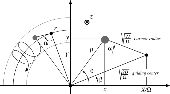
Figure 2: Guiding center $\sqrt{2D/\Omega}$ and Larmor radius $\sqrt{2J/\Omega}$ action variables in a poloidal cross section $(x,y)$.

Then, rather than this Cartesian guiding center variables $X/\Omega$ and $Y$, we will use the polar variables $D$ and $\beta$ obtained through a second canonical transform generated by the generating function of the first type

$$G_{1}\left(Y,\beta\right)=\Omega Y^{2}\cot\left(\beta\right)/2.$$ (12)

The final set of guiding center actions $\left(J,D\right)$ and angles $\left(\alpha,\beta\right)$ variables, illustrated in Fig. 2, can be interpreted as the guiding center polar coordinates $(r=\sqrt{2D/\Omega},\beta)$ and the Larmor radius and cyclotron angle $(\sqrt{2J/\Omega},\alpha)$. They are related to the electron poloidal position $\left(x,y\right)$ through

$$x= \sqrt{\frac{2D}{\Omega}}\cos\beta-\sqrt{\frac{2J}{\Omega}}\cos\alpha,$$

$$y= \sqrt{\frac{2D}{\Omega}}\sin\beta+\sqrt{\frac{2J}{\Omega}}\sin\alpha.$$ (13)

The radial electron coordinate $\rho=\sqrt{x^{2}+y^{2}\text{ }}$can then be written as a function of the angles-actions variable

$$\frac{\Omega}{2}\rho^{2}=D+J-2\sqrt{JD}\cos\left(\alpha+\beta\right).$$ (14)

Introducing the canonical momentum along the magnetic field line $P=\mathbf{p}\cdot\mathbf{e}_{z}$, conjugate to the $z$ variable, we can express the Hamiltonian $H_{0}$ Eq. (10) as

$$H_{0}= ~{}\Omega J+\frac{P^{2}}{2}+\frac{P}{qR}\left[D+J-2\sqrt{JD}\cos\left(\alpha+\beta\right)\right]$$

$$+\frac{1}{2q^{2}R^{2}}\left[D+J-2\sqrt{JD}\cos\left(\alpha+\beta\right)\right]^{2}.$$ (15)

The guiding center poloidal rotation resulting from the helical structure of the field lines is much slower than the cyclotron rotation: $d\alpha/dt=\partial H_{0}/\partial J$ $\approx\Omega$ $\gg d\beta/dt=\partial H_{0}/\partial D$ $\approx P/qR$. This strong ordering allows to safely average the oscillating terms over $\alpha$ as no resonance between $\alpha$ and $\beta$ can take place. The adiabatic Hamiltonian $H_{0}$ describing the guiding center orbits in this adiabatic screw-pinch/straight-tokamak configuration is

$$H_{0}=\Omega J+\frac{P^{2}}{2}+P\frac{J+D}{qR},$$ (16)

where we have neglected the last term on the right hand side since $a/qR<1$.

The physics behind this Hamiltonian is rather simple: (i) $\Omega J$ is the cyclotron rotation energy around the field lines, (ii) $P^{2}/2$ the translation energy along the $z$ direction and (iii) $P\left(J+D\right)/qR$ the kinetic energy associated with the poloidal rotation due to the helicity of the field line. Without collisions or turbulence, $H_{0}$ given by Eq. (16) describes perfect adiabatic confinement such that $dD/dt=dJ/dt=dP/dt=0$.

Within the framework of the turbulent transport driven current problem we are interested by the coupled dynamics of the guiding center radial position $\sqrt{2D/\Omega}$ and the momentum $P$. This coupling is induced by a spectrum of turbulent modes. We will only consider here electrostatic modes and point out that electromagnetic modes described by a perturbating vector potential included in Eq. (10) would yield the same final result.

Consider an electrostatic turbulent spectrum described by the scalar potential

$$\Phi\left(r,\theta,z,t\right)=\sum_{m=-\infty}^{m=+\infty}\sum_{n=-\infty}^{n=+\infty}\Phi_{mn}\left(r\right)\exp\left(jm\theta\right)\exp\left(jn\frac{z}{R}\right)\exp\left(-j\omega_{mn}t\right)$$ (17)

where $\Phi_{mn}\left(r\right)$ is the radial eigenmode associated with the poloidal and toroidal mode $\exp(jm\theta)\exp(jn\varphi)$, with $\theta$ and $\varphi$ ($R\varphi=z$) the poloidal and toroidal angle of the straight tokamak (see Fig. 1), for a given frequency $\omega_{mn}\ll\Omega$. The structure of the radial eigenmode $\Phi_{mn}\left(r\right)$ is very important to set up the various model of tokamak instabilities and turbulence, but it is not needed to derive kinetic theory of transport driven current. We simply assume that it can be decomposed on a natural cylindrical basis of ordinary Bessel functions of order $m$, $J_{m}\left(kr\right)$, and the $k$ Fourier variable can be discrete (Fourier series) if we impose a boundary condition at $r=a$, or continuous otherwise (Fourier integral). The precise nature of this radial expansion does not change the final results of this analytical model of current generation. We thus consider a classical Fourier-Bessel expansion providing a simple identification of resonant transport Watson (1980):

$$\Phi_{mn}\left(r\right)= \int_{0}^{+\infty}kdk\phi_{mn}\left(k\right)J_{m}\left(kr\right);$$

$$\phi_{mn}\left(k\right)= \int_{0}^{+\infty}rdr\Phi_{mn}\left(r\right)J_{m}\left(kr\right)\text{.}$$ (18)

The random phase approximation (RPA) assumes that the effect of each mode can be analyzed separately within the Hamiltonian framework and that the full quasilinear effect is just the sum of these single mode perturbations on the actions averaged over the angles (RPA) Wesson and Campbell (2011); Rax (2014); White (2014). Within this canonical framework let us consider the Hamiltonian $H$ describing the interaction between one electron and one $\left(k,m,n\right)$ mode:

$$H=~{}\Omega J+\frac{P^{2}}{2}+P\frac{J+D}{qR}\\ +\phi_{mn}\left(k\right)J_{m}\left(kr\right)\exp(j[m\theta+n\varphi-\omega_{mn}t]).$$ (19)

This RPA-quasilinear analysis can be further simplified with the help of the Gegenbauer’s addition theorem Watson (1980)

$$J_{m}\left(kr\right)\exp(jm\theta)=\sum_{l=-\infty}^{l=+\infty}J_{l+m}\left(k\sqrt{\frac{2D}{\Omega}}\right)J_{l}\left(k\sqrt{\frac{2J}{\Omega}}\right)\\ \times\exp(jl\alpha)\exp\left[j\left(l+m\right)\beta\right].$$ (20)

This final derivation reduces the analysis of the $\left(k,m,n\right)$ coupling term to a sum over the integer $l$ associated with the order of the cyclotron resonance. For typical electrostatic turbulence $\omega_{mn}\ll\Omega$, so fundamental $l=1$, anomalous $l=-1$ and harmonic $\left|l\right|>1$ cyclotron resonant interactions do not take place. We can then neglect all the components $l\neq 0$ and restrict the model to the $l=0$   component. The low frequency Hamiltonian describing the coupling between the $\left(k,l=0,m,n\right)$ mode and one electron is thus given by

$$H=H_{0}+\phi_{mn}\left(k\right)J_{m}\left(k\sqrt{\frac{2D}{\Omega}}\right)J_{0}\left(k\sqrt{\frac{2J}{\Omega}}\right)\\ \times\exp(jm\beta)\exp(jn\varphi)\exp(-j\omega_{mn}t).$$ (21)

In order to write Hamilton’s equations and to display the breakdown of adiabatic confinement leading to the occurrence of radial transport, we introduce the phase $\Psi_{mn}=m\beta+n\varphi-\omega_{mn}t$   and its unperturbed evolution $\Psi_{mn}\approx\varpi_{mn}t$ with $\varpi_{mn}=mP/qR+nP/R-\omega_{mn}$ to write Hamilton’s equations:

$$\frac{dH}{dt}= \frac{\partial H}{\partial t}=-j\omega_{mn}\phi_{mn}\left(k\right)\mbox{\large$\Xi$}\exp(j\Psi_{mn}),$$ (22)

$$\frac{dD}{dt}= -\frac{\partial H}{\partial\beta}=-jm\phi_{mn}\left(k\right)\mbox{\large$\Xi$}\exp(j\Psi_{mn}),$$ (23)

$$\frac{dP}{dt}= -\frac{\partial H}{R\partial\varphi}=-j\frac{n}{R}\phi_{mn}\left(k\right)\mbox{\large$\Xi$}\exp(j\Psi_{mn}),$$ (24)

with

$$\mbox{\large$\Xi$}=J_{m}\left(k\sqrt{\frac{2D}{\Omega}}\right)J_{0}\left(k\sqrt{\frac{2J}{\Omega}}\right).$$ (25)

Considering the turbulent term $\phi_{mn}$ in Eq. (21) as a perturbation of the adiabatic Hamiltonian $H_{0}$  from Eq. (16) we can integrate these equations during a small time $\delta t$, larger than the period of oscillations of the angles but smaller than the quasilinear evolution of the distribution function in actions space $F\left(J,D,P,t\right)$, in order to get the short time evolution of the energy $H$, the guiding center radial position $D$ and the momentum $P$:

$$\delta H_{kmn}\left(\delta t\right)= -\omega_{mn}\frac{\phi_{mn}}{\varpi_{mn}}\mbox{\large$\Xi$}\exp(j\varpi_{mn}\delta t),$$ (26)

$$\delta D_{kmn}\left(\delta t\right)= -m\frac{\phi_{mn}}{\varpi_{mn}}\mbox{\large$\Xi$}\exp(j\varpi_{mn}\delta t),$$ (27)

$$\delta P_{kmn}\left(\delta t\right)= -\frac{n}{R}\frac{\phi_{mn}}{\varpi_{mn}}\mbox{\large$\Xi$}\exp(j\varpi_{mn}\delta t).$$ (28)

The distribution function in action space at time $t$, $F\left(J,D,P,t\right)$, is the solution of a diffusion equation, the quasilinear equation. The diffusion coefficients of the quasilinear equation are given by the sum over $k$, $m$ and $n$ in Fourier space of the RPA averages

$$\frac{\left\langle\delta{D_{kmn}}^{2}\right\rangle}{2\delta t},$$ (29a)

$$\frac{\left\langle\delta{P_{kmn}}^{2}\right\rangle}{2\delta t},$$ (29b)

and

$$\frac{\left\langle\delta{D_{kmn}}\delta P_{kmn}\right\rangle}{\delta t}$$ (29c)

(we should add a $j\varepsilon$ to the $\varpi_{mn}$ in the denominator to account for causality starting from the past $t=-\infty$). However, there is no need to carry out this standard derivation of the quasilinear theory to derive the kinetic theory of transport driven current in a centrally fuelled discharge. We only need Eqs. (26, 27, 28) to conclude that the ratio of the change of the radial position of the guiding center, $\delta D_{kmn}$, to the increment of momentum along the axial/toroidal direction, $\delta P_{kmn}$, does not depend on $k$ and takes the simple value $Rm/n$ for an $\left(m,n\right)$ mode. Indeed, this relation writes

$$n\delta D_{mn}=Rm\delta P_{mn}.$$ (30)

If we introduce the radial guiding center position $r=\sqrt{2D/\Omega}$ (Fig. 2) such that $\Omega\delta r^{2}=2\delta D_{mn}$ and the parallel velocity $v_{\|}$ such that $m_{e}\delta v_{\|}=$ $\delta P_{mn}$, Eq. (30) rewrites

$$n\Omega r\delta r=mR\delta v_{\|},$$ (31)

which is similar to the heuristic result derived in the introduction. This straightforward and general result is the starting point of the collisional kinetic analysis of the steady-state.

III Kinetic collisional theory of current relaxation

Both the heuristic approach presented in the introduction, and the more rigorous Hamiltonian/RPA theory of section two Eqs. (26, 27, 28), lead to the following conclusion: if a low-frequency turbulent mode with poloidal number $m$ and toroidal number $n$ yields a guiding center radial kick $\delta r$, the elementary step of quasilinear diffusion, then a velocity kick $\delta v_{\|}$ is associated with this incremental radial transport:

$$\delta v_{\|}=\frac{r}{R}\frac{n}{m}\Omega\delta r\text{.}$$ (32)

This fundamental property, used in free energy extraction Fisch and Rax (1992, 1993); Fisch and Herrmann (1994); Heikkinen and Sipil (1995); Herrmann and Fisch (1997); Ochs, Bertelli, and Fisch (2015); Cook, Dendy, and Chapman (2017) and angular momentum injection for advanced tokamak Rax, Gueroult, and Fisch (2017), allows to set up the following physical picture for turbulent transport in a centrally fuelled discharge: an electron starts on the magnetic axis a random walk towards the edge. For every step $\pm\delta r$ it takes along this random walk under the influence of an $\left(m,n\right)$ mode, it gains or looses an incremental momentum $\delta v_{\|}$.

We now recall the concept of electron and hole Rax (1988). An electron with velocity $v_{\|}$, located on the drift surface at radius $r$, jumps on a neighboring drift surface at $r+\delta r$. This is the basic step of the quasilinear random walk. This basic step creates a hole ($h$) in the distribution function at $\left(r,v_{\|}\right)$ and an additional electron ($e$) at $\left(r+\delta r,v_{\|}+\delta v_{\|}\right)$. This electron/hole picture of the quasilinear random walk is shown in Fig. 3 and has been already used to calculate the non-inductive current efficiency Fisch (1987); Rax (1988). Fig. 3 also illustrates the main difference between an edge fuellled and a centrally fuelled discharge. For edge fuelling, the sum of random kicks or radial transport, $\sum_{\text{random walk}}\delta r$, is equal to zero. In contrast, in a centrally fuelled discharge, $\sum_{\text{random walk}}\delta r=a$.

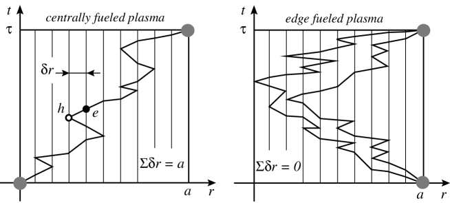
Figure 3: Random walk of an electron from a drift surface $r$ to the next drift surface $r+\delta r$ with central and edge fuelling.

Tokamak experimental results show that the electron population is thermalized and isotropic on drift surfaces, so we consider that collisional thermalization and isotropization are fast processes $\left(\sim 10^{-2}s\right)$ compared with radial transport $\left(\sim 1s\right)$. This strong ordering between collisionless radial transport from drift surface to drift surface and collisional relaxation of the electron and hole excitations justifies the following assumption. The relaxation of the electron/hole is considered as a kinetic process whose initial condition are given by $\left(r,v_{\|}\right)\rightarrow\left(r+\delta r,v_{\|}+\delta v_{\|}\right)$ at time $t=0$ and with no interference with a further quasilinear step $\delta r$ during the isotropization process.

Since we are only interested by the current we can restrict the Landau collisional kinetic equation to pitch-angle scattering on ions. This restriction is also used in the kinetic theory of the Spitzer conductivity for inductive current generation and the kinetic theory of the Fisch efficiency Fisch (1987) for non-inductive current generation.To study the model of Landau collisional relaxation of one hole at $\left(r,v_{\|}\right)$ and one electron at $\left(r+\delta r,v_{\|}+\delta v_{\|}\right)$ we consider a spherical set of coordinates in velocity space directed by the $z$ axis and introduce the pitch-angle of electrons

$$-1\leq\mu=v_{\|}/v\leq+1$$ (33)

where $v=\sqrt{v_{\|}^{2}+v_{c}^{2}}$ is the electron velocity and $v_{c}$ the cyclotron velocity. The distribution function $f_{e/h}\left(r,v,\mu,t\right)$ describes the electron/hole dynamics near the drift surface $r$ resulting from a $\left(\delta r,\delta v_{\|}\right)$ step at $t=0$.

According to Eq. (32) for a given $\left(m,n\right)$ turbulent drive, the evolution of this distribution function $f_{e/h}\left(r,v,\mu,t\right)$ is constrained to take place along quasilinear diffusion paths such that: $Rm\delta\left(v\mu\right)=\Omega rn\delta r$. Going back to the actions evolutions given in Eqs. (26, 27, 28), the ratio of the RPA energy kick Eq. (26) to the parallel momentum kick Eq. (28) is given by $\delta H/\delta D=\delta v^{2}/2\Omega r\delta r=\omega_{mn}/m$. In spherical coordinates $v_{\|}=v\mu$  and the velocity space modification associated with a radial step $\delta r$ under the influence of an $\left(m,n\right)$ mode is thus described by the pitch angle kick

$$\delta\mu_{mn}=\Omega\frac{r}{R}\frac{\delta r}{v}\left(\frac{n}{m}-\mu\frac{\omega_{mn}R}{mv}\right)\text{.}$$ (34)

As we will ultimately average over a Maxwellian distribution for$\ v$, we will not consider the energy slowing down and diffusion and we concentrate on pitch-angle scattering which preserves $v$ owing to the large ion to electron mass ratio. We introduce the classical collision time Wesson and Campbell (2011) $\tau$ defined as

$$\tau\left(v,r\right)=\frac{8\pi{\varepsilon_{0}}^{2}{m_{e}}^{2}v^{3}}{e^{4}n_{e}\left(r\right)\log\Lambda}\text{,}$$ (35)

and the effective ion charge state $Z$. The fast collisional decay of an electron-hole excitation $v\mu_{0}\rightarrow v\left(\mu_{0}+\delta\mu_{mn}\right)$ created at time $t=0$ near $r$ is described by the kinetic equations Fisch (1987); Rax (1988)

$$\left[\frac{\partial}{\partial t}-\frac{Z+1}{\tau}\frac{\partial}{\partial\mu}\left(1-\mu^{2}\right)\frac{\partial}{\partial\mu}\right]\text{ }f_{h}\left(r,\mu,t\right)\\ =-\delta\left(\mu-\mu_{0}\right)\delta\left(t\right),$$ (36)

$$\left[\frac{\partial}{\partial t}-\frac{Z+1}{\tau}\frac{\partial}{\partial\mu}\left(1-\mu^{2}\right)\frac{\partial}{\partial\mu}\right]\text{ }f_{e}\left(r+\delta r,\mu,t\right)\\ =\delta\left(\mu-\mu_{0}-\delta\mu_{mn}\right)\delta\left(t\right)\text{,}$$ (37)

where $\delta\left(t\right)$ and $\delta\left(\mu-\mu_{mn}\right)$ are Dirac distributions and $\delta\mu_{mn}$ the RPA kick Eq. (34) induced by an $\left(m,n\right)$ drive. We can neglect the gradient of the collision time as the elementary step $\delta r$ is far smaller than $a$, and define the electron/hole excitation: $g\left(r,\mu,\mu_{0},t\right)=f_{e}\left(r,\mu,t\right)+f_{h}\left(r,\mu,t\right)$. This electron-hole distribution function is solution to the kinetic equation:

$$\left[\frac{\partial}{\partial t}-\frac{Z+1}{\tau}\frac{\partial}{\partial\mu}\left(1-\mu^{2}\right)\frac{\partial}{\partial\mu}\right]\text{ }g\left(r,\mu,\mu_{0},t\right)\\ =\delta\mu_{mn}\frac{d\delta\left(\mu-\mu_{0}\right)}{d\mu_{0}}\delta\left(t\right)\text{.}$$ (38)

To solve this kinetic equation we expand the electron-hole excitation $g$ over the Legendre polynomials $P_{l}\left(\mu\right)$ which are the classical basis to study electron anisotropy in plasma kinetic problems such as the Spitzer conductivity problem or the Fisch efficiency problem. The Dirac pitch-angle source $\delta\left(\mu-\mu_{o}\right)$ can be expanded as

$$\delta\left(\mu-\mu_{o}\right)=\sum_{l=0}^{l=+\infty}\frac{2l+1}{2}P_{l}\left(\mu\right)P_{l}\left(\mu_{o}\right)\text{.}$$ (39)

The Legendre polynomials are the eigenfunctions of the pitch-angle isotropization kinetic operator:

$$\left[\frac{\partial}{\partial\mu}\left(1-\mu^{2}\right)\frac{\partial}{\partial\mu}\right]P_{l}\left(\mu\right)+l\left(l+1\right)P_{l}\left(\mu\right)=0\text{.}$$ (40)

These two relations, Eq. (39,40), allow to solve analytically the Landau kinetic equation Eq. (38). The various anisotropic components decay exponentially and

$$g\left(r,\mu,\mu_{0},t\right)=H\left(t\right)\delta\mu_{mn}\sum_{l=1}^{l=+\infty}\frac{2l+1}{2}\exp\left[-l\left(l+1\right)\left(Z+1\right)\frac{t}{\tau}\right]P_{l}\left(\mu\right)P_{l}^{\prime}\left(\mu_{o}\right),$$ (41)

where $H\left(t\right)$ is the Heaviside step function such that $H\left(t\geq 0\right)=1$ and $H\left(t<0\right)=0$ and the prime indicates a derivative with respect to $\mu_{0}$.

In a centrally fuelled steady-state tokamak, with a single $\left(m,n\right)$ turbulent mode, during a time $dt$, an average number of electrons $dN=W_{f}dt/Q_{DT}$ jump from $r$ to $r+\delta r$. As all the electrons are equally involved, the distribution of $\mu_{0}$ variable is flat between $-1$ and $+1$, so the steady-state non-equilibrium pitch-angle distribution $G_{nm}\left(r,\mu\right)$ at radius $r$ is given by the average:

$$G_{nm}\left(r,\mu\right)= \int gd\mu_{0}dN$$

$$= \frac{W_{f}}{Q_{DT}}\int_{-1}^{+1}d\mu_{0}\int_{-\infty}^{+\infty}g\left(r,\mu,\mu_{0},t\right)dt.$$ (42)

The Legendre polynomials expansion Eq. (41) provides the final result as a sum of odd and even components:

$$G_{nm}\left(r,\mu\right)=\frac{W_{f}}{Q_{DT}}\frac{r\delta r}{Rv}\tau\left[\sum_{l=1,3,5...}\frac{n\left(2l+1\right)}{ml\left(l+1\right)\left(Z+1\right)}P_{l}\left(\mu\right)-\sum_{l=2,4,6...}\frac{\omega_{mn}R\left(2l+1\right)}{ml\left(l+1\right)\left(Z+1\right)v}P_{l}\left(\mu\right)\right]\text{.}$$ (43)

The current $\delta I_{nm}\left(r\right)$ associated with steady-state electron/hole excitations by a single $\left(n,m\right)$ mode is given by the $v_{\|}=v\mu$ moment of the $G_{nm}\left(r,\mu\right)$ non-equilibrium distribution function

$$\delta I_{nm}\left(r,\delta r\right)= \frac{e}{2\pi R}\int_{-1}^{+1}v\mu G_{mn}\left(r,\mu\right)d\mu$$

$$= \frac{e}{2\pi R}\frac{\Omega W_{f}}{Q_{DT}R}\frac{n}{m}\frac{r\tau}{\left(Z+1\right)}\delta r\text{.}$$ (44)

If the tokamak is fuelled from the edge

$$\sum_{\text{random walk}}\delta r=0\quad\textrm{and}\quad\sum_{\text{random walk}}\delta I_{mn}=0,$$ (45)

whereas if the tokamak is centrally fuelled

$$\sum_{\text{random walk}}\delta r=a\quad\textrm{and}\quad\sum_{\text{random walk}}\delta I_{mn}\neq 0.$$ (46)

The expression of the full transport driven current associated with the mode $\left(m,n\right)$ must be averaged over a Maxwellian distribution of the velocity $v$ with temperature $T_{e}\left(r\right)$ and then integrated from the center to the edge ($\sum\delta r=\int dr$) with respect to the random radial walk:

$$I_{nm}= \sum_{\delta r}\left\langle\delta I_{mn}\left(r,\delta r\right)\right\rangle_{T_{e}\left(r\right)}$$

$$= \frac{e}{2\pi\left(Z+1\right)}\frac{\Omega W_{f}}{Q_{DT}R^{2}}\frac{n}{m}\int_{0}^{a}drr\left\langle\tau\left(v,r\right)\right\rangle_{T_{e}\left(r\right)}\text{.}$$ (47)

We introduce the mean collision time $\left\langle\tau\right\rangle$ as an average over velocity and radial position according to the relation:

$$\left\langle\tau\right\rangle= \frac{\int_{0}^{a}r\left\langle\tau\left(v,r\right)\right\rangle_{T_{e}\left(r\right)}dr}{a^{2}/2}$$

$$= \frac{64{\varepsilon_{0}}^{2}\sqrt{2\pi m_{e}}{k_{B}}^{3/2}}{e^{4}a^{2}\log\Lambda}\int_{0}^{a}\frac{T_{e}\left(r\right)^{\frac{3}{2}}}{n_{e}\left(r\right)}rdr\text{,}$$ (48)

so that the $\left(m,n\right)$ driven current is

$$\frac{I_{mn}}{W_{f}}=\frac{\left\langle\tau\right\rangle\Omega}{2\pi\left(Z+1\right)}\frac{e}{Q_{DT}}\frac{a^{2}}{R^{2}}\frac{n}{m}\text{.}$$ (49)

This relation assumes that a single $\left(n,m\right)$ mode is at work to provide the radial collisionless transport of the electrons from $r=0$ to $r=a$. In fact, the turbulent activity of a discharge is associated with a spectrum of $\ m$ and $n$ and we have to define a mean spectral characteristic of the discharge to express the transport driven current.

IV Discussion and conclusion

As we work within the framework of the RPA, we can sum the effects of each $\left(m,n\right)$ mode and neglect the interferences between the various modes Wesson and Campbell (2011); Rax (2011); Kaufman (1972); White (2014). As identified and discussed at the end of Sec. II, each $\left(m,n\right)$ mode contributes to the full quasilinear radial diffusion coefficients $\left\langle\delta{D_{kmn}}^{2}\right\rangle$/$2\delta t$ and $\left\langle\delta D_{kmn}\delta P_{kmn}\right\rangle$/$2\delta t$. Specifically, Eqs. (26, 27, 28) show that the contribution of mode $(m,n)$ is proportional to ${\phi_{mn}}^{2}$. Thus we introduce a coefficient proportional to ${\phi_{mn}}^{2}$ measuring the relative contribution of each $\left(m,n\right)$ mode to quasilinear diffusion in $\left(J,D,P\right)$ space, that is to say to current generation. The final formulae for the full transport driven current $I$ is thus given by

$$\frac{I}{W_{f}}=\frac{\Omega\left\langle\tau\right\rangle}{2\pi\left(Z+1\right)}\frac{e}{Q_{DT}}\frac{a^{2}}{R^{2}}\left\langle\frac{n}{m}\right\rangle\text{,}$$ (50)

where we have defined the mean ratio of toroidal to poloidal mode number $\left\langle n/m\right\rangle$ as

$$\left\langle\frac{n}{m}\right\rangle=\sum_{m=-\infty}^{m=+\infty}\sum_{n=-\infty}^{n=+\infty}\frac{n}{m}\int_{0}^{+\infty}kdk\frac{{\phi_{mn}}^{2}\left(k\right)}{\sum_{m,n=-\infty}^{m,n=+\infty}\int_{0}^{+\infty}udu{\phi_{mn}}^{2}\left(u\right)}.$$ (51)

There is no poloidally isotropic mode $\phi_{0n}=0$ in the spectrum and the energy ${\phi_{mn}}^{2}$ content of each mode reflects its contribution to radial quasilinear transport.

Equation (50), which quantifies the transport driven current $I$, was derived under two hypotheses. First, the interaction between an electron and electrostatic modes has been assumed to be governed by RPA quasilinear transport, as supported by the careful identification of the slow action and the fast phases of the adiabatic motion as given in Sec. II. Second, it has been assumed in Sec. III that collisional relaxation is consistent with Landau kinetic theory. To the extent that these two frameworks are the standard descriptions for mode-particle and particle-particle interactions in tokamak physics Wesson and Campbell (2011); Rax (2011), the final relation Eq. (50) is valid within the regime of applicability of these approaches. However, note that if, for example, anomalous electron transport arises from magnetic turbulence along random magnetic field lines Rechester and Rosenbluth (1978); Rax and White (1992), then this model of electrostatic turbulence and the effect of transport driven current described by Eq. (50) are no longer valid.

In order to provide a general simple scaling we consider that the radial temperature and density profiles are characterized by an exponent $\gamma$ such that

$$\frac{T_{e}\left(r\right)^{\frac{3}{2}}}{n_{e}\left(r\right)}=\frac{{T_{0}}^{\frac{3}{2}}}{n_{0}}\left(1-\frac{r^{2}}{a^{2}}\right)^{\gamma}\text{,}$$ (52)

where $T_{0}$ is the electron temperature on the magnetic axis and $n_{0}$ the electron density on axis. With this profile Eq. (52) the mean relaxation time $\left\langle\tau\right\rangle$ Eq. (48) becomes

$$\left\langle\tau\right\rangle=\frac{32{\varepsilon_{0}}^{2}\sqrt{2\pi m_{e}}}{\left(\gamma+1\right)e^{5/2}\log\Lambda n_{0}}\left(\frac{k_{B}T_{0}}{e}\right)^{\frac{3}{2}}.$$ (53)

Plugging Eq.(53) into Eq.(50), we get the scaling of the transport current as a function of the plasma parameters for a centrally fuelled cylindrical thermonuclear discharge:

$$\frac{I}{W_{f}}\left[\frac{\text{A}}{\text{W}}\right]\approx\frac{3}{\left(Z+1\right)\left(\gamma+1\right)\log\Lambda}\frac{a^{2}}{R^{2}}\left\langle\frac{n}{m}\right\rangle\left[\frac{B}{1\text{ T}}\right]\\ \times\left[\frac{k_{B}T_{0}/e}{1\text{ kV}}\right]^{\frac{3}{2}}\left[\frac{10^{13}\text{ cm}^{-3}}{n_{0}}\right]\text{.}$$ (54)

Equations (50,54) are the main original results of this study.

The only unknown parameter in this relation is $\left\langle n/m\right\rangle$ defined in Eq. (51). In tokamaks, unstable modes feeding the turbulence spectrum are localized near resonant drift surface associated with closed helical field lines. This motivates us to assume here that $\left\langle n/m\right\rangle\sim 1/q$, where $q$ is the mean safety factor of the discharge. However, the validity of this last hypothesis should be confirmed in future studies. Indeed, if the electrostatic spectrum were to be such that $\left\langle n/m\right\rangle\sim 0$, then the effect would be much weaker. It is worth noting here though that the coefficient involved in Eq. (50) is not $\left\langle n\right\rangle$ or $\left\langle m\right\rangle$ separately but $\left\langle n/m\right\rangle$.

For typical ITER parameters, and assuming $\left\langle n/m\right\rangle\sim 1/q$, Eq. (54) predicts a transport driven current of few mega-amperes which confirms the favorable scaling already identified in Sec. I. This remains true even if accounting for trapped particles. Indeed, introducing the fraction of passing particles $P_{e}\left(r\right)=1-\sqrt{2r/R}$ on the drift surface $r$, the kinetic analytical model can be extended by substituting the the radial average

$$\left\langle\tau\right\rangle=\frac{64{\varepsilon_{0}}^{2}\sqrt{2\pi m_{e}}{k_{B}}^{3/2}}{e^{4}a^{2}\log\Lambda}\int_{0}^{a}P_{e}\left(r\right)\frac{T_{e}\left(r\right)^{\frac{3}{2}}}{n_{e}\left(r\right)}rdr\text{,}$$ (55)

in lieu of Eq. (48). With the general radial profile

$$P_{e}\left(r\right)\frac{T_{e}\left(r\right)^{\frac{3}{2}}}{n_{e}\left(r\right)}=\left(1-\sqrt{\frac{2r}{R}}\right)\frac{{T_{0}}^{\frac{3}{2}}}{n_{0}}\left(1-\frac{r^{2}}{a^{2}}\right)^{\gamma},$$ (56)

the $I/W_{f}$ expression in Eq. (54) is then multiplied by the correcting factor:

$$0<1-\frac{\left(1+\gamma\right)\Gamma\left(\gamma+1\right)\Gamma\left(5/4\right)}{\Gamma\left(\gamma+9/4\right)}\sqrt{\frac{2a}{R}}<1\text{,}$$ (57)

where $\Gamma$ is the gamma function defined by Euler’s integral $\Gamma\left(u\right)=$ $\int_{0}^{+\infty}t^{u-1}\exp\left(-t\right)dt$. As anticipated, this correction does not change the order of magnitude for $I$ and just lower the cylindrical result by a factor one half to one third depending on $\gamma$.

It is to be noted that transport driven current suffers from a drawback similar to the bootstrap current: the current on the magnetic axis cancels. This transport driven current effect can be interpreted as a slight preferential loss of electrons traveling in the direction of the toroidal current under the hypothesis of a centrally fuelled discharge.

In summary, we have identified, described and analyzed the transport driven current due to central fuelling in cylindrical and toroidal discharges. The interplay between current generation and radial transport was explored with a phenomenological model in Ref. Rax and Moreau (1989) or within the framework of magnetic turbulence in Ref. Rax, Robiche, and Kostyukov (1999). However, these studies did not take into account the consequences of the quasilinear hypothesis Eq. (34) and the central fuelling hypothesis, and hence missed this effect. Ref. Nunan and Dawson (1994) reports the first observation of this effect but is restricted to 2+1/2 dimensional electromagnetic, particle-in-cell simulations. The original analytical kinetic theory presented in this study is supported by these early results in the collisionless regime. However, and although the first-principles mechanisms are similar, direct comparison of the current is not possible because of the electron to ion mass ratio used in these particle-in-cell studies.

The first-principles analytical kinetic model derived in this paper is based on two standard assumptions: (i) collisional relaxation of anisotropy (current) is faster than anomalous radial transport and (ii) tokamak kinetics is described by quasilinear and Landau equations. This suggests that the final cylindrical scaling Eq. (50) and toroidal correction factor Eq. (57) are robust results. On the other hand, what must be improved through further studies is the prediction of the order of magnitude $\left\langle n/m\right\rangle$ defined in Eq. (51).

The main result of this quasilinear/collisional model is Eq. (50), which can can be summarized as follows. If the requirements of central fuelling and typical turbulent spectrum $\left\langle n/m\right\rangle\sim 1/q$ were to be satisfied in an ITER discharge, an additional, transport driven, current of up to a few mega-amperes is predicted besides the bootstrap and non-inductive currents. This additional current would improve the global power balance of a steady-state burning plasma.

References

References

- Wesson and Campbell (2011) J. Wesson and D. J. Campbell, Tokamaks (Oxford University Press, Oxford, 2011).
- Rax (2011) J.-M. Rax, Physique des tokamaks ( d. de l’ cole polytechnique, Paris, 2011).
- Fisch (2014) N. J. Fisch, Fusion Sci. Technol. 65, 1 (2014).
- Fisch (1978) N. J. Fisch, Phys. Rev. Lett. 41, 873 (1978).
- Fisch (1987) N. J. Fisch, Rev. Mod. Phys. 59, 175 (1987).
- Bickerton, Connor, and Taylor (1971) R. J. Bickerton, J. W. Connor, and J. B. Taylor, Nature Phys. Sci. 229, 110 (1971).
- Kadomtsev and Shafranov (1971) B. Kadomtsev and V. Shafranov, in Proceedings of the Fourth International Conference on Plasma Physics and Controlled Nuclear Fusion Research, Madison, WI, USA, Vol. 2 (International Atomic Energy Agency, Vienna, 1971) p. 479.
- Nunan and Dawson (1994) W. J. Nunan and J. M. Dawson, Phys. Rev. Lett. 73, 1628 (1994).
- Ma and Dawson (1994) S. Ma and J. M. Dawson, Phys. Plasmas 1, 2661 (1994).
- Galeev and Sagdeev (1968) A. A. Galeev and R. Z. Sagdeev, Sov. Phys. JETP 26, 233 (1968).
- Kaufman (1972) A. N. Kaufman, Phys. Fluids 15, 1063 (1972).
- Robiche and Rax (2004) J. Robiche and J. M. Rax, Phys. Rev. E 70, 046405 (2004).
- Ware (1970) A. A. Ware, Phys. Rev. Lett. 25, 916 (1970).
- Rax and Moreau (1989) J. M. Rax and D. Moreau, Nucl. Fusion 29, 1751 (1989).
- Rax (2014) J. M. Rax, Fusion Sci. Technol. 65, 10 (2014).
- Fisch and Rax (1992) N. J. Fisch and J.-M. Rax, Phys. Rev. Lett. 69, 612 (1992).
- Fisch and Rax (1993) N. J. Fisch and J.-M. Rax, Phys. Fluids B 5, 1754 (1993).
- Fisch and Herrmann (1994) N. Fisch and M. Herrmann, Nucl. Fusion 34, 1541 (1994).
- Heikkinen and Sipil (1995) J. A. Heikkinen and S. K. Sipil , Phys. Plasmas 2, 3724 (1995).
- Herrmann and Fisch (1997) M. C. Herrmann and N. J. Fisch, Phys. Rev. Lett. 79, 1495 (1997).
- Ochs, Bertelli, and Fisch (2015) I. E. Ochs, N. Bertelli, and N. J. Fisch, Phys. Plasmas 22, 112103 (2015).
- Cook, Dendy, and Chapman (2017) J. Cook, R. Dendy, and S. Chapman, Phys. Rev. Lett. 118, 185001 (2017).
- Rax, Gueroult, and Fisch (2017) J. M. Rax, R. Gueroult, and N. J. Fisch, Phys. Plasmas 24, 032504 (2017).
- White (2014) R. B. White, The Theory of Toroidally Confined Plasmas, 3rd ed. (Imperial College Press, 2014).
- Watson (1980) G. N. Watson, A Treatise on the Theory of Bessel Functions (Cambridge University Press, New York, NY, 1980).
- Rax (1988) J. M. Rax, Phys. Fluids 31, 1111 (1988).
- Rechester and Rosenbluth (1978) A. B. Rechester and M. N. Rosenbluth, Phys. Rev. Lett. 40, 38 (1978).
- Rax and White (1992) J. M. Rax and R. B. White, Phys. Rev. Lett. 68, 1523 (1992).
- Rax, Robiche, and Kostyukov (1999) J. M. Rax, J. Robiche, and I. Kostyukov, Phys. Plasmas 6, 3233 (1999).