Parallel tree algorithms for AMR
and non-standard data access

Abstract

We introduce several parallel algorithms operating on a distributed forest of adaptive quadtrees/octrees. They are targeted at large-scale applications relying on data layouts that are more complex than required for standard finite elements, such as $hp$-adaptive Galerkin methods, particle tracking and semi-Lagrangian schemes, and in-situ post-processing and visualization. Specifically, we design algorithms to derive an adapted worker forest based on sparse data, to identify owner processes in a top-down search of remote objects, and to allow for variable process counts and per-element data sizes in partitioning and parallel file I/O. We demonstrate the algorithms’ usability and performance in the context of a particle tracking example that we scale to 21e9 particles and 64Ki MPI processes on the Juqueen supercomputer, and we describe the construction of a parallel assembly of variably sized spheres in space creating up to 768e9 elements on the Juwels supercomputer.

1 Introduction

Numerical methods to solve partial differential equations (PDEs) have become ubiquitous in science and industry. Many approaches subdivide the domain of the PDE into a mesh of cells that constitute the computational elements. The finite/spectral element/volume methods are among the most prevalent techniques and establish mathematical links between nearest-neighbor elements; see e.g. [52, 6, 3, 19, 41, 24]. This concept is tremendously useful to realize parallel computing, where each process works on a subregion of the mesh, and their coupling is implemented by communicating data only between processes that hold adjacent elements.

For some applications, however, nearest-neighbor-only communication is an undesired constraint. This applies to element-based particle tracking, such as the particle/marker-in-cell methods [32, 33], used for example in plasma physics [20] or viscoelasticity [45], to semi-Lagrangian methods such as [21], and to smoothed particle hydrodynamics [28] and molecular dynamics [23]. Here the mathematical design allows for moving numerical information by more than one mesh element per time step. If this is attempted in practice, new ideas are needed to locate points on non-neighbor remote elements and to find their assigned process. If the “points” are extended geometric objects that can stretch across more than one element/process, such as in rigid body dynamics [47], an algorithm must cope with multivalued results.

Another generalization of the above-mentioned classic methods is the association of variably sized data to elements. An obvious example is the $hp$-adaptive finite element method [53], where the data size for an element depends on its degree of approximation. More generally, we may think of multiple phases or sub-processes, say physical or chemical, that differ locally in their data usage. We may also think of selecting a subset of elements for processing while ignoring the rest, which can be useful for visualization (visible vs. non-visible [25]) or file-based output (relevant vs. irrelevant according to a user). Efficiently and adaptively managing such data and repartitioning it between processes is nontrivial.

In this paper, we present several new high level algorithms as well as low level building blocks that perform the operations motivated above. With “high level” we refer to algorithms that appear as a well-defined black box to the calling code, hiding any kind of mathematical intricacy and specialty logic on the inside. Our focus is on (a) highly scalable methods that (b) operate on dynamically adaptive meshes. Targeting simulations that run on present-day supercomputers, allowing for meshes that adapt every few, each, or even several times per time step, requires a carefully designed logical organization of the elements. To support efficient searches and to aid in creation and partitioning of data, we choose a combination of a distributed tree hierarchy and a linear ordering of elements via a space filling curve (SFC) [56, 55]. To allow for general geometries, we generalize to a forest of one or more trees [51, 8, 17].

1.1 Proposed algorithms

We understand the proposed algorithms as tools that may be relied upon by conceptually higher-level codes, middleware and libraries, and also by application developers requiring any of the features offered. While the following description is abstract and general, the reader is encouraged to visit Sections 6 and 7 for concrete, illustrated examples in the context of numerical simulations.

Sparse construction

The first algorithm, presented in Section 3, serves to derive a custom worker mesh in a direct one-pass algorithm, which reduces the run time over the common procedure of calling multiple cycles of global refinement and coarsening. This can be useful in material simulations to create an independent forest adapted to one subsystem (say a fracture zone). Another use would be to create a worker forest for just the camera-visible elements within an in-situ visualization algorithm. These worker forests can be partitionend independently from the source forest to run their specific task while preserving overall load-balance. Our algorithm is sort-free and has sub-second run times throughout. This improves over bottom-up constructions from scratch [55], which have their merit when such heavier functionality is required by the application, by a large margin.

Remote process search

In Section 4, we propose a top-down algorithm to find non-local generalized points in the domain. These “points” may be actual points or particles, extended geometric objects, or arbitrarily shaped regions in space. “Non-local” means that we find the precise intersection of each point with the set of process subdomains. The algorithm has the following key features. 1. We search for multiple points in one pass to amortize mesh memory access, and we enable multiple match elements/processes per point. 2. We enable both optimistic matching (for example to use fast bounding-box checks closer to the root) and early discarding (to prune search subtrees as quickly as possible). 3. We match points to subtrees on remote processes, even though we do not have access to any remote element (ghost or otherwise). In fact, the whole algorithm is local and communication-free. This ostensible paradox is resolved due to our lightweight yet complete encoding of the forest’s partition.

Partitioning and parallel I/O

When writing data to permanent storage, it is an advantage for testing and general reproducibility if the output format is independent of the number of processes und the partition of elements that has been used to compute it. While devising such a format for a single tree is not hard, it becomes more involved for a forest encoded with minimal metadata. Another problem related to partitioning is the transfer of fixed- and variable-sized per-element data, which most applications will allocate in their own memory space. For this data, no direct repartitioning interface has been available so far. We propose two minimal parallel algorithms that perform these tasks in Section 5.

1.2 Related work

The need for particle tracking is fundamental in astrophysics and molecular dynamics simulations. The use of tree codes for this purpose goes back a long time [34, 43]. It has been found effective to sort the points by interpreting their tree location relative to a space filling curve [49, 57]. Such functionality is not always custom coded. The FLASH code, for example, delegates the search of remote particles to the mesh library [22], while the Chombo library as one such candidate exposes a formal interface for specifying particle locations [2]. The Gadget3 code uses a Hilbert curve [48], and its feature to form groups of nearby particles for aggregated searching has been introduced similarly in the molecular dynamics code GROMACS [1].

Our algorithms are designed to satisfy the needs of all of the above codes. In addition, we provide more generality in several respects, where one is that we (a) allow for searching objects of positive diameter that may each intersect with more than one process domain, which can be useful in rigid body dynamics and visualization. Another important aspect of the present work is that we do (b) not rely on a single- or multi-width ghost layer or halo region. Such reliance has frequently been found problematic in all areas from astrophysics [37] to smoothed particle hydrodynamics [57] and molecular dynamics [29].

For efficiency and flexibility, we (c) support grouping in the spirit of [39], which offers multiple and optimistic matching as well as early pruning of search subtrees. Encouraged by use cases [4], we design our algorithms such that we (d) require no data transformation [5], no duplication of data structures [44], and no parallel sorting [55]. Last but not least, our algorithms enable (e) large scale dynamic adaptive meshing and repartitioning with sub-second absolute run times.

One of our goals is to avoid communication issues due to MPI_Alltoall, busy MPI wait loops, or overallocation of buffers, and we make an effort to calculate known sender and receiver ranks and message sizes. In doing so, we find that our algorithms are ideally suited to produce the exact meta information needed for precise point-to-point communication. This information is similarly fitting for setting up active synchronization in one-sided MPI [36], such that we support both models.

1.3 Examples and reproducibility

Particle tracking example

In Section 6, we develop an element-based scheme that solves Newton’s equations of motion for a large number of non-interacting particles. The elements are refined, coarsened, and partitioned dynamically to keep the number of particles per element near a specified number. Especially the non-local search of points is crucial to redistribute the particles to the elements/processes after their positions are updated.

Remote search example

In Section 7, we detail the parallel construction of randomly distributed spheres, implementing a non-local refinement criterion by the use of the proposed algorithms. This approach guarantees a pseudo-random, configurable mesh refinement that does not depend on the number of processes used to create it. Thus, we establish and demonstrate partition-independence as an explicit invariant.

Software

We provide a reference implementation of all algorithms and example programs as part of the p4est software library [9]. p4est is an MPI-only code, where multiple compute cores per hardware node are transparently supported by spawning the appropriate amount of MPI ranks. Explicit shared-memory versions of our algorithms may be written, yet would add little to the logic we expose in this document—instead, we rely on optimized shared-memory MPI performance [42]. We use the prefix p4est_ for functions that can be found in the software under the same or a similar name, while unprefixed subroutines serve to clarify the exposition. We take special care to be explicit about the less obvious mathematical conventions and tricks that are synergetic to the p4est design, which will allow the reader to reimplement all algorithms in their own code.

In-situ visualization

We refer the interested reader to [10] for an extended discussion of parallel visualization algorithms based on the functionality exposed in this paper.

2 Principles and conventions

Our algorithms do not rely on nearest neighbor relations but on the SFC order that defines and encodes the parallel partition. As a benefit, the algorithms presented here share the property that the forest need not be 2:1 balanced and that they do not depend on a ghost layer. We abstain from incremental tree encodings [7] to ensure that all elements are individually accessible.

While we maintain the notion of elements, they need not necessarily refer to a classical finite element or a numerical solver context. We allow for arbitrary-size application data to be redistributed in parallel in the same optimized way that is used for the adaptive mesh, which opens up the performance and scalability established for managing meshes [12, 39] to many sorts of data. We hint at various examples and use cases in the respective sections of this paper.

Throughout the paper, we will be dealing with integers exclusively. When referring to integer intervals $[a,b)\cap\mathbb{Z}$, we omit the intersection for brevity. All arrays are 0-based. Cumulative arrays (i.e., arrays storing partial sums) are typeset in uppercase fraktur ($\mathfrak{E}$). We denote the number of parallel processes (MPI ranks) by $P$, the number of trees in the forest of octrees by $K$, and the global number of elements (leaves of the forest) by $N$. Thus, a process number reads $p\in[0,P)$ and a tree number $k\in[0,K)$.

2.1 Cycles of adaptation

In a typical adaptive numerical simulation, the mesh evolves between time steps in cycles of mesh refinement and coarsening (RC), mesh balancing and/or smoothing (B), and repartition (P) for load balancing. Not to be confused with the latter, mesh balancing may refer to establishing a 2:1 size condition between direct neighbor elements [56, 55, 17, 38] and mesh smoothing to establishing a graded transition in the sizes of more or less nearby elements. After RC+B, the new mesh exists in the same partition boundaries as the previous one, while families of four (2D) or eight (3D) sibling elements have been replaced by their parent, or vice versa. We note that refinement and coarsening is rarely applied recursively, except for example during the initialization phase of a simulation.

Since RC+B changes the number of elements independently on each process, load balance is lost, and P redistributes the elements in parallel to reinstate it. To guarantee that one cycle of coarsening is always possible, the partition algorithm may be modified to place every sibling of one family on the same process [54]. In some applications it may be beneficial to partition before refinement, possibly using weights depending on refinement and coarsening indicators, in order to avoid crashes when one process refines every local element and runs out of memory. P is complementary to RC+B in the sense that it changes the partition boundary while the elements stay the same. This design ensures modularity between and flexible combination of individual algorithms and simplifies the projection and transfer of simulation data [13, Figures 3 and 4]:

Principle 1 (Complementarity principle).

A collective mesh operation shall either change the local element sizes within the existing partition boundary, or change the partition boundary and keep the elements the same, but not both.

It should be noted that time stepping is not the only motivation to use adaptivity: When utmost accuracy of a single numerical solve is required, we may use a-posteriori error estimation to refine and solve the same problem repeatedly at successively higher resolutions; when setting up a geometric multigrid solver, we create a hierarchy of coarser versions of a mesh. In both scenarios, we may add mesh smoothing and most definitely repartitioning at each level of resolution using the same RC+B+P algorithms, which is key for the scalability of geometric/algebraic solvers [14, 54, 50].

2.2 Encoding a parallel forest

We briefly introduce the relevant properties of the p4est data structures and algorithms [17], which we see in this paper as a reference implementation of an abstract forest of octrees. We consider a forest that is two- or three-dimensional, $d=2$ or $3$, which generalizes easily to arbitrary dimensions. The topology of a forest is defined by its connectivity, i.e., an enumeration of tree roots viewed as cubes mapped into $\mathbb{R}^{3}$ together with a specification of each one’s neighbor trees across the tree faces, edges (in 3D), and corners. Neighbor relations include the face/edge/corner number as viewed from the neighbor and a relative orientation, since the coordinate systems of touching trees need not align.

The mesh primitives in p4est are quadrilaterals in 2D and hexahedra in 3D. They arise as leaves of a quadtree (2D) or octree (3D), where a root can be subdivided (refined) into $2^{d}$ child branches (subtrees). The subdivision can be performed recursively on the subtrees. For simplicity, we will use the term “quadrant” for a tree node. A quadrant is either a branch quadrant (it has child quadrants) or it is a leaf quadrant. The root quadrant is a leaf if the tree is not refined and a branch otherwise. We call leaves in both 2D and 3D the elements of the adaptive mesh.

In practice, we limit the subdivision to a maximum depth or level $L$, where the root is at level $\ell=0$. Accordingly, a quadrant is uniquely defined by the tree it belongs to, the coordinates $(x_{i})=(x,y,z)$ of its lower left front corner, each an integer in $[0,2^{L})$, and its level $\ell\in[0,L]$. A quadrant of level $\ell$ has integer edge length $2^{L-\ell}$, and its coordinates are integer multiples of this length. We assume that a space filling curve (SFC) is defined that maps all possible quadrants of a given level bijectively into an ordered set of curve indices $[0,2^{d\ell})$. We may always embed this index into the space $[0,2^{dL})$ by left-shifting by $d(L-\ell)$ bits. The level may be appended to the curve index to make the index unique across all levels.

The order defined by the SFC must satisfy a locality property: The children of a quadrant are called a family and have indices that come after any predecessor and before any successor of their parent quadrant. As a consequence, two quadrants are either related as ancestor and descendant, meaning that the latter is contained in the former, or not intersecting at all: Partially overlapping quadrants do not exist. Common choices of SFC are the Hilbert curve [35] and the Morton- or $z$-curve [46] used in p4est. In fact, the algorithms in this paper are equally fit to operate on a forest of triangles or tetrahedra, as long as its connectivity is well defined and it is equipped with an SFC such as the one designed for the t8code [15].

A forest is stored in a data object that exists on each participating process. Most of its data members are local, that is, apply to just the process where they are stored, while others are shared, meaning that their values are identical between all processes. The shared data is minimal such that it uniquely defines the parallel partition. We use linearized tree storage that only stores the leaves and ignores the non-leaf nodes [55]. The leaves are ordered in sequence of the trees, and within each tree in sequence of the SFC order. Sometimes we reference local data for the tree with global number $k$ inside a forest object $s$ by $\mathcal{K}=s.\mathrm{trees}[k]$.

The partition of leaves is disjoint, which allows us to speak of the owning process of an element. For convenience, the local data of each process includes the numbers of its first and last non-empty trees. The trees between and including its first and last are called its local trees. The first and last trees of a process may be incomplete, in which case the remaining elements belong to preceding processes for the first, and to succeeding processes for the last local tree. If a process has more than two trees, the middle ones must be complete. If a process has elements of only one tree, its first and last tree are the same. In this case, if that tree is incomplete, its remaining elements may be on processes both preceding and succeeding. A process may also be empty, that is, have no elements, in which case it has no valid first and last tree.

For each of its local trees, a process stores an offset defined by the sum of local elements over all preceding trees, and the tree’s boundaries by way of its first and last local descendants. The first (last) local descendant is the first (last) descendant of maximum level $L$ of its first (last) local element in this tree. For example, the first local descendant of a complete tree in Morton encoding has coordinates $x_{i}=0$, while the last has coordinates $x_{i}=2^{L}-1$, $i\in[0,d)$. The local elements are stored in one flat array for each local tree. Thus, the tree number for every local element is implicit. Non-local elements are not stored.

The shared data of the forest is the array $\mathfrak{E}[p]$, the sum of local elements over all preceding processes, and the array $\mathfrak{m}[p].(\mathrm{tree},\mathrm{desc})$ of the first local tree and local descendant, for every process $p$. The first local descendant of a process is identical to the first local descendant of its first tree. Consequently, the array of first descendants is sufficient to recreate the first and last local descendants $\mathcal{K}.f$, $\mathcal{K}.l$ of any tree local to any process. We call $\mathfrak{m}$ the array of partition markers, since they define the partition boundary in its entirety (see Figure 1).

By design of the SFC, the entries of $\mathfrak{m}$ are ascending first by tree and then by the index of the first local descendant. Whether a process begins with a given tree and quadrant, even if the quadrant is non-local and/or a branch, is trivial to check by examining $\mathfrak{m}$; see Algorithm 1 and its use from Algorithm 9 and Algorithm 12.

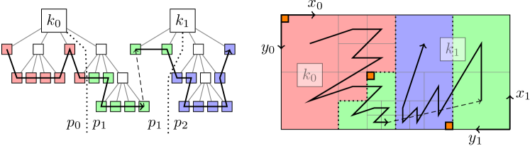
Fig. 1: Sketch of a forest of $K=2$ quadtrees $k_{i}=i$ (left) and the mesh it encodes (right). Each tree in the mesh has its own coordinate system that determines the order of elements along the space filling curve (black arrows). The forest is partitioned between $P=3$ processes $p_{j}\equiv j$ (color coded). The partition markers $\mathfrak{m}[0,1,2]$ (orange) are quadrants of a fixed maximum level; we do not draw $\mathfrak{m}[3]$. They correspond to the black dotted lines on the left that are sometimes called separators [30]. This forest is load balanced with cumulative element counts $\mathfrak{E}=[0,7,15,23]$.

Algorithm 1 begins_with (process $p$, tree number $k$, quadrant $b$)

Determine in $\mathcal{O}(1)$ whether a hypothetical quadrant in a specific tree is the first quadrant on some process $p$. This function showcases use of the marker array $\mathfrak{m}$.

0:  $b$ is a quadrant in tree $k$ {omit tree “number” from now on}

1:  return  $\mathfrak{m}[p]=(k,\text{first descendant of $b$})$ {comparison yields true or false}

As stated above, the arrays $\mathfrak{E}$ and $\mathfrak{m}$ are available to each process, a feature that is crucial throughout. It has been found exceedingly convenient to store one additional element in these zero-based arrays, namely $\mathfrak{E}[P]$ and $\mathfrak{m}[P]$. Quite naturally, $\mathfrak{E}[P]$ is the global number of elements, and the number of elements on process $p$ is $\mathfrak{E}[p+1]-\mathfrak{E}[p]$ for all $p\in[0,P)$. Setting $\mathfrak{m}[P]$ to the first descendant of the non-existent tree $K$ permits to encode any empty process $p$, including the last one, by $\mathfrak{m}[p]=\mathfrak{m}[p+1]$, that is, by successive partition markers being equal in both tree and descendant. If one or several successive processes are empty, we say that all of them begin on the same tree and quadrant as the next non-empty process. By design, Algorithm 1 returns true for all of them.

It follows from the above conventions that the array $\mathfrak{m}$ contains information on the ownership of trees as well:

Property 2.

Not every tree needs to occur in $\mathfrak{m}$.

If $k$ occurs and the range of processes $[p,q]$ is widest such that begins_with ($p^{\prime}$, $k$, $b$) for all $p\leq p^{\prime}\leq q$ and the same $b$, and $p$ is the first satisfying this condition for any $b$, then the first descendant of tree $k$ is in the partition of either $p-1$ or $q$. More specifically, it is $q$ if and only if begins_with ($q$, $k$, $\mathrm{root}$).

If $k$ does not occur in $\mathfrak{m}$, then all of its quadrants are owned by the last process $p$ that satisfies $\mathfrak{m}[p].\mathrm{tree}<k$.

3 Forest construction from sparse leaves

In many use cases an application must construct a mesh for which only a small subset of current elements is relevant:

• To isolate elements of a given refinement level (and fill the gaps with the coarsest possible elements to complete the mesh), for example to implement multigrid or local time stepping.

• To postprocess only the mesh elements selected by a given filter (such as for writing to disk the data of one part of a much bigger model).

• A computation deals with points distributed independently of the element partition and varying strongly in density, and we seek to create a mesh representing the points.

• For parallel visualization, we want to process only the part of the mesh inside the view angle of a virtual camera.

Repeated coarsening addresses only some of these cases and is unnecessarily slow when it does: We would execute multiple cycles and carefully maintain data consistency between them. Coarsening may also be inadequate entirely, such as in the case of points where we might want to create a highly refined element for each one, potentially finer than in the original mesh.

The operation we need is akin to making a copy of the existing mesh (we will keep the original and its data to continue with the simulation eventually), and then executing multiple cycles of RC+P on the copy, all in a fast one-pass design. In particular, we want to avoid creating forest metadata or element storage and discarding it again.

While some details in this section are new, the presentation is more of a tutorial in working with our mathematical encoding of a parallel forest of octrees. This section also serves to introduce some subalgorithms required later.

3.1 Algorithmic concept

We propose the following procedure p4est_build:

1. Initialize an opaque context data structure from an existing source forest that will hide temporary working data (Algorithm 2, p4est_build_begin).

2. Add leaves one by one, which need not exist in the source mesh (i.e., they may be coarser or finer) but must be contained in the local partition, and must be non-overlapping and their index non-decreasing relative to the ones added previously. These leaves can be sparse (that is, not contiguous in the order of the space filling curve; cf. Algorithm 6, p4est_build_add).

3. Free the context, not before creating a new forest object as a result: It is defined as the coarsest possible forest (a) containing the added leaves and (b) respecting the same partition (Algorithm 7, p4est_build_end).

The resulting forest has the same partition boundary as the source, thus the above procedure satisfies Principle 1.

One advantage is that the construction is process-local, with the caveat that the result depends on the total number of processes. However, since the result is a valid forest object, it can be subjected to calls to RC+B if so desired, and P in order to load balance it for its special purpose. Its number of elements may be smaller than that of the source, possibly by orders of magnitude, significantly accelerating the computation downstream.

As a difference to [55], we use a source forest to guide the algorithm. The monotonicitiy requirement, to add leaves in the order of the source index, eliminates the linear-logarithmic runtime of a sorting step. Monotonicity can be realized for example by iterating through the existing leaves in the source, or by calling the top-down forest traversal p4est_search. The latter approach has the advantage that the traversal can be pruned early to skip tree branches of no interest, not accessing these source elements at all.

p4est_build shares the property of p4est_search that the serial version is useful in itself, since the tasks mentioned above may well occur in a single-process code. The parallel version of p4est_build is near identical to the serial one, with the exception that the local number of leaves in the result, one integer, is shared with MPI_Allgather. This is standard procedure in p4est for refinement, coarsening, and 2:1 balance. Apart from that, the algorithm is communication-free.

3.2 Details description of p4est_build

Algorithm 2 p4est_build_begin (source forest $s$) $\rightarrow$ context $c$ (collective call)

This algorithm is the entry point to the sparse construction of a forest. We record a reference to the original forest and initialize context information to maintain state.

1:  $c\leftarrow$ new context storing reference to $s$ and new and empty result forest $r$

2:  if $s$ has elements on this process then

3:     begin_tree ($c$, $s.\mathrm{first\_local\_tree}$, $0$) {set $c.\mathrm{most\_recently\_added}\leftarrow\mathrm{is\_invalid}$}

4:  end if

We use a context data structure to track the internal state of building the new forest from an ascending (and usually sparse) set of local leaves. It is initialized by p4est_build_begin (Algorithm 2) and contains a copy of the variables of the source forest that stay the same, most importantly the boundaries of local trees plus the array of partition markers. These copies become parts of the result forest at the end of the procedure. In practice, redundant data may be avoided by copy-on-write. The state information contains the number of the tree currently being visited and a copy of the most recently added element, which serves to verify that a newly added element is of a larger SFC index and not overlapping (Algorithm 6, Line 5).

In adding elements, we pass through the local trees in order. When adding multiple elements to one tree, we cache them and postpone the final processing of this tree until we see an element added to a higher tree for the first time. If at least one element has been added to the tree, we can rely on the functions p4est_complete_subtree, originally built around a fragment of CompleteOctree [55, Algorithm 4, lines 16–19] and reworked [38], and p4est_complete_region, a reimplementation of the function CompleteRegion originally described for Dendro [55, Algorithm 3]. Both functions are adapted to the multi-tree data structures of p4est and parameterized by the number of the tree to work on.

Algorithm 3 p4est_enlarge_first (quadrant $f$ is modified, quadrant $b$)

Given a quadrant $f$, we determine whether it is a first child and strictly contained in $b$. If so, we turn it into its parent and repeat. This preserves the lower left corner of $f$.

0:  $f$ is descendant of $b$ (i.e., equal to $b$ or a strict descendant of it)

1:  $w=f.x\operatorname{|}f.y\operatorname{|}f.z$ {bitwise or; omit $z$ coordinate in 2D}

2:  while $f.\ell>b.\ell$ and ($w\operatorname{\&}2^{L-f.\ell})=0$ do

3:     $f.\ell\leftarrow f.\ell-1$ {turn $f$ into parent; valid due to $=0$ comparison in Line 2 }

4:  end while

4:  $f$ has the same first descendant as on input and is still descendant of $b$

Algorithm 4 p4est_enlarge_last (quadrant $l$ is modified, quadrant $b$)

This algorithm is the complement to Algorithm 3 in that the last (top right back) corner of $l$ is preserved during repeated enlargement of the quadrant.

1:  $\ell\leftarrow l.\ell$; $w=l.x\operatorname{\&}l.y\operatorname{\&}l.z$ {bitwise and; omit $z$ coordinate in 2D}

2:  while $l.\ell>b.\ell$ and ($w\operatorname{\&}2^{L-l.\ell})\neq 0$ do

3:     $l.\ell\leftarrow l.\ell-1$ {turn $l$ into parent; requires Line 5 to become well defined}

4:  end while

5:  $l.x\leftarrow l.x\operatorname{\&}\neg(2^{L-l.\ell}-2^{L-\ell})$ {bitwise negation; repeat for $y$ (and $z$ in 3D)}

5:  $l$ has the same last descendant as on input and is still descendant of $b$

Algorithm 5 end_tree (context $c$) $\rightarrow$ element offset $o$

In our loop over the local trees of the source forest, we transfer the temporary data recorded by adding sparse quadrants into the tree structure of the result forest.

1:  $\mathcal{K}\leftarrow c.r.\mathrm{trees}[c.k]$ {reference to result tree data}

2:  if $\mathcal{K}.\mathrm{elements}=\emptyset$ then

3:     $a\leftarrow$ p4est_nearest_common_ancestor ($\mathcal{K}.f$, $\mathcal{K}.l$)

4:     if $\mathcal{K}.f$ is the first descendant of $a$ and $\mathcal{K}.l$ is its last then

5:        $\mathcal{K}.\mathrm{elements}\leftarrow\{a\}$ {tree consists of one element}

6:     else

7:        $f\leftarrow\mathcal{K}.f$; $l\leftarrow\mathcal{K}.l$ {first and last local descendants of tree}

8:        $c\leftarrow$ child of $a$ containing $f$; p4est_enlarge_first ($f$, $c$); {modify $f$}

9:        $d\leftarrow$ child of $a$ containing $l$; p4est_enlarge_last ($l$, $d$); {modify $l$}

10:        p4est_complete_region ($\mathcal{K}$, $f$, $l$) {fill elements in $\mathcal{K}$ from $f$ to $l$ inclusive}

11:     end if

12:  else

13:     p4est_complete_subtree ($\mathcal{K}$) {fill gaps with coarsest possible elements}

14:  end if

15:  return  $\mathcal{K}.o+\#\mathcal{K}.\mathrm{elements}$

In the event that no element has added to some local tree, we fill the range between its first and last local descendants with the coarsest possible elements. To this end, we first generate the smallest common ancestor of the two descendants, which contains the local portion of the tree. If the tree descendants are equal to the ancestor’s first and last descendants, respectively, the ancestor is the tree’s only element. Otherwise, we identify the two (necessarily distinct) children of the ancestor that contain one of the tree descendants each, and find the descendants’ respective largest possible ancestor that (a) has the same first (last) descendant and (b) is not larger than the child. We do this with Algorithm 3 p4est_enlarge_first and Algorithm 4 p4est_enlarge_last, respectively. We then call p4est_complete_region with the resulting elements to fill the tree.

The finalization of a tree for the cases discussed above is listed in Algorithm 5. The reader may notice that the logic in Lines 8 and 9, along with the enlargement algorithms, could be tightened further by passing just the number $a.\ell+1$ instead of the children $c$ and $d$. We omit such final optimizations in p4est when not harmful to its performance, since the information on the child quadrants is valuable for checking the consistency of the code.

Algorithm 6 p4est_build_add (context $c$, tree $k$, quadrant $b$, callback Add)

Between p4est_build_begin and p4est_build_end we may add individual sparse quadrants that need neither be contiguous nor existing in the source forest.

0:  $c.k\leq k\leq c.s.\mathrm{last\_local\_tree}$ {adding element to same or higher tree}

1:  while $c.k<k$ do

2:     $o\leftarrow$ end_tree ($c$) {finalize current tree, adding its elements to offset}

3:     begin_tree ($c$, $c.k+1$, $o$) {commence the next tree}

4:  end while

5:  if $c.\mathrm{most\_recently\_added}\neq\mathrm{is\_invalid}$ then

5:     $c.\mathrm{most\_recently\_added}$ less equal and not an ancestor of $b$

6:     if $c.\mathrm{most\_recently\_added}=b$ then

7:        return  {convenient exception allows for redundant adding}

8:     end if

9:  end if

10:  $\mathcal{K}.\mathrm{elements}\leftarrow\mathcal{K}.\mathrm{elements}\cup\{b\}$ {sparse leaves in tree structure until finalized}

11:  $c.\mathrm{most\_recently\_added}\leftarrow b$ ; Add ($b$) {optionally initialize application data}

We allow to call the p4est_build_add function repeatedly with the same element, which is a convenience when using the feature of p4est_search to maintain a list of multiple points to search [39], several of which may trigger the addition of the current element. A new element may just as well be finer or coarser than the one in the source, as long as it is added in order. The element is added once, and we provide the convenience callback Add to establish its application data; see Algorithm 6.

Algorithm 7 p4est_build_end (context $c$) $\rightarrow$ result forest $r$ (collective call)

Tansfer the rest of the temporary context data into the result forest and finalize it.

1:  if $c.s$ has elements on this process (else $n\leftarrow 0$) then

2:     while $c.k<c.s.\mathrm{last\_local\_tree}$ do

3:        begin_tree ($c$, $c.k+1$, end_tree ($c$)) {finalize and commence as above}

4:     end while

5:     local element count $n\leftarrow$ end_tree ($c$) {we are done with the last local tree}

6:  end if

7:  $c.r.\mathrm{numbers}\leftarrow$ MPI_Allgather ($n$) {one integer per process}

8:  return  $c.r$ {also free $c$’s remaining members and $c$ itself}

4 Recursive partition search

Frequently, points or geometrically more complex objects need to be located relative to a mesh. The task is to identify one or several elements touching, intersecting, or otherwise relevant to that object. There are varied examples of such objects and their uses:

• Input/output:

  • Earthquake point sources to feed energy into seismology simulations

  • Sea buoys for measuring the water level in tsunami simulations

• Numerical/technical:

  • Particle locations in tracer advection schemes

  • Departure points in a semi-Lagrangian method

• Geometric shapes:

  • Randomly distributed grains to construct a porous medium

  • Trapezoids that represent the field of view of a virtual camera

  • Constructive solid geometry objects for rigid body interactions

In the following, we refer to all those objects as points. We distinguish three degrees of generality required depending on the application.

1. Local: When it suffices that each process shall identify strictly the points that are inside its local partition, we may call p4est_search [39, Algorithm 3.1] to accomplish this task economically and communication-free.

2. Near: The points are searched in a specified proximity around the local partition. For example, in most numerical applications we work with direct neighbors in the mesh. Usually we collect one layer of ghost elements that encode the size, position, and owner process of direct remote neighbors. If the ghost elements are ordered by the SFC, they can be searched very much like the local elements [17]. This principle can be extended to multiple layers of ghosts [31, p4est_ghost_expand ]. However, the number of ghost layers must be limited, since the number of ghost elements collected on any given process cannot be much larger than the number of local elements due to memory constraints.

3. Global: Every process may potentially ask for the location of every point. This variant is clearly the most challenging, since a naive implementation would cause $\mathcal{O}(P^{2})$ work and/or all-to-all communication.

This section is dedicated to develop a lean and general solution of the global problem 3. The main task of the new Algorithm 10, p4est_search_partition, is to identify which points match the local partition and which do not, and in the latter case, which process(es) they match. It will be advantageous to follow the forest structure top-down to reduce the number of binary searches and to tighten their ranges as much as possible. To avoid traversing the forest more than once, we use the top-down context over all relevant points as a whole. Given the metadata we hold for the forest, the algorithm is communication-free.

While an all-to-all parallel search is not expected to scale, our approach is efficient when the application requires data that is near in a generalized sense but not accessible by Local and Near searches. If, for example, we search through a neighborhood in space that extends to a small multiple of the width of a process domain, such as in a large-CFL Lagrangian method, we prune the search for the domain outside of the neighborhood and the procedure scales well.

4.1 Idea of the recursion

We know that the local part of the search can be executed using p4est_search. Assuming we remembered all points that do not match locally and run two nested loops to search each of those points on every remote process, this would be rather costly. The alternative of sorting the coordinates of the points in order of the SFC and comparing it with the partition markers is not applicable when the points are extended geometric shapes. Instead, we repurpose the idea behind p4est_search and apply it to the partition markers instead of the local quadrants. This inspires a top-down traversal of the partition of the forest without accessing any element (which would be impossible anyway, since remote elements are generally unknown to a given process).

To illustrate the principle, consider a branch quadrant of a given tree and assume that we know the process that owns its first local descendant and the one that owns its last. These two processes define the relevant window onto the array of partition markers. Hence, we are done if the first and last process are identical: This is the owner of all leaves below the branch. Otherwise, we split the branch quadrant into its $2^{d}$ children and look for them in the window of partition markers using a multi-target binary search. This gives us for each child its first and last process, which allows us to continue this thought recursively, using each child in turn as the current branch.

The above procedure has several useful properties. First, to bootstrap the recursion, we execute a loop over all (importantly, not just the local) trees since a point may exist in any tree. The partition markers allow us to determine for each tree which processes own elements of it. The ascending order of trees, processes, and partition markers inherent in the SFC allows us to walk through this information quickly. Furthermore, a leaf can only have one owner process, which means that the recursion is guaranteed to terminate on a leaf, if not before, even when this leaf is remote and thus not known to the current process.

Second, we process all points in one common recursion, which combined with per-point user decisions of whether it intersects the branch allows us to prune the search tree early and only follow the relevant points further down. Both the search window and the set of relevant points shrink with increasing depth of the branch. Finally, it is possible to do optimistic matching, meaning returning matches for a point and more than one branch, which may allow for cheaper match queries in practice. Any sharp and more costly matching can be delayed if this is advantageous. The motivation for this is quite natural in view of searching extended geometric shapes that may overlap with more than one process partition. We illustrate the process in Figure 2.

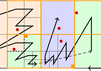
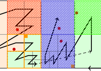
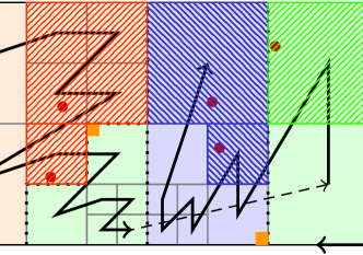
Fig. 2: Steps of p4est_search_partition on process $2$ (blue; cf. Figure 1), which must locate 5 points (red), 3 of which are not local. Top left: recursion at level 1 after 5 search quadrants (orange) have returned true in Match. Top right: The red quadrant is remote and the recursion stops at the branch containing the point. The green quadrant is remote and coincides with a leaf, and the recursion stops. The two blue quadrants are local, one branch and one leaf, and the recursion stops. The recursion continues with 4 level 2 quadrants (orange). Bottom left: Final result; one search quadrant matches on the red process. Bottom right: Alternate result obtained by an extension akin to p4est_search, making use of the local leaves as a convenience (blue hatched backwards).

4.2 Technical description of p4est_search_partition

As outlined in Section 2.2, p4est stores one partition marker per process that contains the number of its first tree. To find the processes relevant for each tree, we need to reverse this map. In principle, we could run one binary search per tree to find the smallest process that owns a part of it. Instead of doing this and spending $K\log P$ time, we can exploit the ascending order of both trees and processes, and the fact that the range of processes for a tree is contiguous, to run the combined and optimized multi-target search sc_array_split presented in [39]. We restate the precise convention for its input and output parameters in Algorithm 8.

Algorithm 8 sc_array_split (input array $\mathfrak{a}$, offset array $\mathfrak{O}$, number of types $T$)

Interface to multi-objective binary search over a cumulative array developed in [39].

0:  $\mathfrak{a}$ is sorted ascending by some type $0\leq\mathfrak{a}[i].t<T$ (repetitions allowed)

0:  $\mathfrak{O}$ has $T+1$ entries to be computed by this function

0:  The positions $i$ of $\mathfrak{a}$ that hold entries of type $t$ are $\mathfrak{O}[t]\leq i<\mathfrak{O}[t+1]$

0:  If there are no entries of type $t$ in $\mathfrak{a}$, then $\mathfrak{O}[t]=\mathfrak{O}[t+1]$

To create the map from tree to process, we use the partition markers $\mathfrak{m}$ as input array $\mathfrak{a}$. We exploit the fact that it has $P+1$ entries and there is $P^{\prime}$ minimal such that $\mathfrak{m}[p^{\prime}].\mathrm{tree}=K$ for all $p^{\prime}\in[P^{\prime},P]$. Usually, we have $P^{\prime}=P$, but me way also encounter the case $P^{\prime}<P$ if the final range of processes $p\in[P^{\prime},P)$ has no elements und hence no trees. Designating the tree number of the partition marker as the type for sc_array_split, we see that we must specify $T=K+1$ types and the offset array $\mathfrak{O}$ must have $K+2$ entries. Algorithm 8 gives us

$$\mathfrak{O}[0]=0,\quad\mathfrak{O}[K]=P^{\prime}\leq P,\quad\text{and}\quad\mathfrak{O}[K+1]=P+1.$$ (1)

Now, running the loop over all trees $0\leq k<K$, we need to determine the first and last processes $p_{\mathrm{first}}$, $p_{\mathrm{last}}$ owning elements of tree $k$. We know for a fact that

$$p_{\mathrm{last}}=\mathfrak{O}[k+1]-1.$$ (2)

This can be seen since $p_{\mathrm{last}}\geq\mathfrak{O}[k+1]$ would mean that $p_{\mathrm{last}}$ could not have any elements of trees $k$ and less. And if there were a $p^{\prime}$ with $p_{\mathrm{last}}<p^{\prime}<\mathfrak{O}[k+1]$, then $p_{\mathrm{last}}$ would not be the last process of tree $k$. To determine $p_{\mathrm{first}}$, we distinguish the cases of (a) no process beginning in this tree, (b) a process begins at its first descendant, and (c) a process begins elsewhere in $k$. We name this algorithm processes (Algorithm 9) and call it with the the type $t=k$ and the root quadrant of the tree.

Algorithm 9 processes (offset array $\mathfrak{O}$, type $t$, quadrant $b$) $\rightarrow$ ($p_{\mathrm{first}}$, $p_{\mathrm{last}}$)

Given an offset array of process ranks classified by some type (depending on the calling context, for example the first tree of a process or the first child index relative to a search quadrant), determine the tightest inclusive range of processes of this type.

0:  By context, $b$ is a quadrant in some tree $k$

1:  $p_{\mathrm{last}}\leftarrow\mathfrak{O}[t+1]-1$ {this value is final}

2:  $p_{\mathrm{first}}\leftarrow\mathfrak{O}[t]$ {initialization}

3:  if $p_{\mathrm{first}}\leq p_{\mathrm{last}}$ and begins_with ($p_{\mathrm{first}}$, $k$, $b$) then

4:     while $p_{\mathrm{first}}$ is empty do

5:        $p_{\mathrm{first}}\hskip 0.43057pt\text{$++$}$ {empty processes use same type as their successor}

6:     end while

7:  else

8:     $p_{\mathrm{first}}\hskip 0.43057pt\text{$--$}$ {there must be exactly one earlier process for this type}

9:  end if

9:  Range $[p_{\mathrm{first}},p_{\mathrm{last}}]$ is widest s.t. each end has at least one item of type $t$

We show the toplevel call p4est_search_partition in Algorithm 10. For clarity, we have excluded the local search of points (covered in detail in [39]) and reduced the presentation to the search over the parallel partition. Since it does not communicate, it can be called by any process at any time. It identifies the relevant processes for each tree in turn as discussed above and then invokes the recursion for each tree. The recursion keeps track of the points to be searched by a user-defined callback function Match. This callback is passed the range of processes relevant for the current branch quadrant and may return false to indicate an early termination of the recursion. The points and the callback to query them do not need to relate to invocations on other processes.

Algorithm 10 p4est_search_partition (point set $Q$, callback Match)

Toplevel interface for generalized partition search. We use the multi-objective binary search to bootstrap the range of relevant trees, and we make sure that the range of processes per tree is tight (Algorithms 8 and 9) before entering the per-tree recursion.

1:  sc_array_split ($\mathfrak{m}$, $\mathfrak{O}$, $K+1$) {split partition markers $\mathfrak{m}$ by their tree number}

2:  for all tree numbers $0\leq k<K$ do

3:     $a\leftarrow\mathrm{root}$ {construct toplevel quadrant to begin}

4:     ($p_{\mathrm{first}}$, $p_{\mathrm{last}}$) $\leftarrow$ processes ($\mathfrak{O}$, $k$, $a$) {potential owners of quadrants in $k$}

5:     recursion ($a$, $p_{\mathrm{first}}$, $p_{\mathrm{last}}$, $Q$, Match) {bootstrap recursion for tree $k$}

6:  end for

The recursion is detailed in Algorithm 11. Each step takes a branch quadrant $b$ and the first and last processes that own elements of it. If they are the same, this is the owner of all elements below $b$ and the recursion ends. Otherwise, the task is to find the first and last processes $p_{i,\mathrm{first}}$ and $p_{i,\mathrm{last}}$ for each child $c_{i}$ of $b$. Here we use sc_array_split with an input array that is the minimal window on the markers, defined by

$$\mathfrak{a}[j]=\mathfrak{m}[p_{\mathrm{first}}+1+j]\quad\text{for}\quad 0\leq j<\Delta p=p_{\mathrm{last}}-p_{\mathrm{first}}.$$ (3)

This ensures that all elements of $\mathfrak{a}$ refer to processes beginning inside $b$. We set their type to the number of the child of $b$ in which they begin, which fixes $T=2^{d}$ and yields

$$\mathfrak{O}[0]\geq 0,\quad\mathfrak{O}[2^{d}]=\Delta p,\quad\text{and}\quad p_{i,\mathrm{last}}=\mathfrak{O}[i+1]+p_{\mathrm{first}}.$$ (4)

If we want to repurpose processes to determine $p_{i,\mathrm{first}}$ and $p_{i,\mathrm{last}}$, we need to make sure that the offset array indexes into processes, which we accomplish by adding $p_{\mathrm{first}}+1$ to each of its elements (Line 12) to correct for the window selection (3).

Algorithm 11 recursion
(quadrant $b$, processes $p_{\mathrm{first}}$, $p_{\mathrm{last}}$, point set $Q$, callback Match)

Recursion step of the partition search. It is allowed for the callback to match without knowing whether this match is final. Note that we traverse each subtree at most once.

0:  By context, $b$ is a quadrant in some tree $k$

0:  The first descendant of $b$ is owned by $p_{\mathrm{first}}$, its last by $p_{\mathrm{last}}$

1:  Set of matched points $M\leftarrow\emptyset$

2:  for all $q\in Q$ do

3:     if Match ($b$, $p_{\mathrm{first}}$, $p_{\mathrm{last}}$, $q$) then

4:        $M\leftarrow M\cup\{q\}$ {determine the points that we keep}

5:     end if

6:  end for

7:  if $M=\emptyset$ or $p_{\mathrm{first}}=p_{\mathrm{last}}$ then

8:     return  since all matches failed and/or all quadrants below $b$ belong to $p_{\mathrm{first}}$

9:  end if

10:  sc_array_split ($\mathfrak{m}[p_{\mathrm{first}}+1,\ldots,p_{\mathrm{last}}]$, $\mathfrak{O}$, $2^{d}$) {split by child id relative to $b$}

11:  for all $c_{i}\in\texttt{Children}$ ($b$), $0\leq i<2^{d}$ do

12:     ($p_{i,\mathrm{first}}$, $p_{i,\mathrm{last}}$) $\leftarrow$ processes ($\mathfrak{O}+p_{\mathrm{first}}+1$, $i$, $c_{i}$) {owning descendants of $c_{i}$}

13:     recursion ($c_{i}$, $p_{i,\mathrm{first}}$, $p_{i,\mathrm{last}}$, $M$, Match) {pursue remaining points to bottom}

14:  end for

5 Partitioning and parallel I/O

This section introduces parallel algorithms that support partition-independent storage of the mesh and the communication of application data between an old and new parallel partition. One guideline that we follow throughout is the following.

Principle 3 (partition independence).

On writing, the organization and contents of file(s) written for a given state of data shall be independent of the parallel partition of the simulation. On reading, any number of processes shall be suitable to read such a file (provided that the total memory available is sufficient).

Partition independence is a valuable idea for a multitude of reasons, such as:

1. Data is often transferred to a different computer for post-processing, having a different number of processors and a different runtime/batch system.

2. The scalability of post-processing algorithms is usually less than that of simulation algorithms.

3. We would like to make regression-testing, reproduction and post-processing least restrictive and most convenient further down the data processing chain.

5.1 Writing element counts per tree

The element counts per tree are a partition-invariant property of a global forest mesh and thus important to define a concise and complete mesh I/O format. However, they are not maintained within the internal state of the parallel forest, which prompts us to develop a dedicated algorithm to compute them using minimal time and communication.

Let us first consider the (simpler) situation of a one-tree forest. If we were to include $P$ and the arrays $\mathfrak{m}$ and $\mathfrak{E}$ in the mesh file, it would not be partition independent. Thus, the only header information permitted is the global element count $N=\mathfrak{E}[P]$. In practice, it is written by the first process, but any other process would be able to write the header as well. For each element we store its coordinates $x_{i}$ and the level, which are of fixed size $s$. The window of the mesh file to be written by process $p$ is

$$\text{size of header }+s\times[\mathfrak{E}[p],\mathfrak{E}[p+1]),$$ (5)

which is easily done in parallel using the MPI I/O standard. On reading, each process learns the values $p$ and $P$ from the MPI environment and reads the header to learn $N$. This is sufficient to compute a new array $\mathfrak{E}$ [17, equation (2.5)], which is in turn sufficient to read the local elements from the file by (5). The first element read fixes the local partition marker $\mathfrak{m}[p]$, while an empty process sets it to an invalid state. The partition markers are shared by one call to MPI_Allgather and examined once to repair the invalid entries due to empty processes.

For a multi-tree forest, we encounter two additional tasks. The first is writing the number of trees and their connectivity to the file, for which we exploit the fact that the connectivity is known to each process in the current p4est design. The second task is deeper: When reading the window of local elements, it is not known which tree(s) they belong to. Of course, we may store the tree number in each element, but this would be redundant and add some dozen percent to the file size. One way to encode the tree assignment of elements efficiently is to postulate an array $\mathfrak{N}$ of cumulative global element counts over trees and to include it in the header.

Let $N_{k}>0$ be the global number of elements in tree $k$ that is generally not available from the distributed data structure. Our goal is to compute these counts and encode them in a cumulative array $\mathfrak{N}$ with $K+1$ non-decreasing entries,

$$.\mathfrak{N}[k^{\prime}]=\sum_{k=0}^{<k^{\prime}}N_{k},\quad 0\leq k^{\prime}\leq K\qquad\Rightarrow$$ (6a)

$$\mathfrak{N}[0]=0,\qquad\mathfrak{N}[k+1]-\mathfrak{N}[k]=N_{k}\>,\qquad\mathfrak{N}[K]=\sum_{k=0}^{<K}N_{k}=N.$$ (6b)

This format is convenient in facilitating binary searches through the results. Note that any $N_{k}$ may be greater equal $2^{32}$ and thus requires 64 bits of storage.

We aim to avoid the communication and computation cost $\mathcal{O}(KP)$ of a naive implementation, i.e., one that has every process count the elements in every tree. Our proposal is to define a unique process responsible for computing the element count in any given tree, and to minimize communication by sending at most one message per process to obtain the counts. This shall hold even if a process is responsible for more than one tree. Multiple conventions are thinkable to decide on the responsible process, where we demand that the decision is made without communication. We also demand that all pairs of sender and receiver processes are decided without communication. One suitable choice is the following.

Convention 4.

The process $p$ responsible for computing the number of elements in tree $k$, which we denote by $p_{k}$, is the one that owns the first element in $k$, unless more than one process has the first descendant of tree $k$ as their partition marker. In the latter case, we take $p_{k}$ as the first process in that set, which is necessarily empty.

This convention ensures that the range of trees that a process is responsible for is contiguous (or empty). In addition, it guarantees that $k<k^{\prime}$ implies $p_{k}\leq p_{k^{\prime}}$. Allowing for empty processes to be responsible fixes $p_{0}=0$ in all cases.

Property 5.

An empty process is responsible for at most one tree.

Proof.

If an empty process were responsible for two different trees, both would have to occur in its partition marker, which is impossible by definition. ∎

Let us proceed by listing the phases of the algorithm $\mathfrak{N}\leftarrow\texttt{p4est\_\-count\_\-pertree}$.

1. Determine for each process $p$ the number of trees that it is responsible for,

   $$K_{p}=\#\{k:p_{k}=p\},\qquad 0\leq K_{p}\leq K.$$ (7)

   We may additionally define an array $\mathfrak{K}$ of cumulative counts,

   $$\mathfrak{K}[p^{\prime}]=\sum_{p=0}^{<p^{\prime}}K_{p}\qquad\Rightarrow\qquad\mathfrak{K}[0]=0,\qquad\mathfrak{K}[P]=K.$$ (8)

   Due to the design of the partition markers and Convention 4, every process populates these arrays identically in $\mathcal{O}(\max\{K,P\})$ time, requiring no communication. We provide Algorithm 12 to detail this computation.

   Algorithm 12 responsible (computes arrays of tree counts $(K_{p})$, tree offsets $\mathfrak{K}$)

   Compute which processes are responsible for counting elements in which trees. This is a process-local preparation for establishing the global per-tree element counts.
   

   1:  $p\leftarrow 0$; $k\leftarrow 0$; $K_{0}\leftarrow 0$

   2:  loop

   2:     Process $p$ is the minimum of all $p^{\prime}$ with $k=\mathfrak{m}[p^{\prime}].\mathrm{tree}$ (cf. Property 2)

   2:     Responsibility for $k$ has been assigned to either $p$ or $p-1$

   3:     repeat

   4:        $p\hskip 0.43057pt\text{$++$}$; $K_{p}\leftarrow 0$ {find the first process that begins in a later tree}

   5:     until $\mathfrak{m}[p].\mathrm{tree}>k$

   6:     $k\hskip 0.43057pt\text{$++$}$ {proceed to that tree incrementally}

   7:     while $k<\mathfrak{m}[p].\mathrm{tree}$ do

   8:        $K_{p-1}\hskip 0.43057pt\text{$++$}$; $k\hskip 0.43057pt\text{$++$}$ {while assigning in-between trees}

   9:     end while

   10:     if $k=K$ then

   11:        $K_{p^{\prime}}\leftarrow 0$ forall $p^{\prime}\in[p+1,P)$; break loop {assign remaining slots}

   12:     else if begins_with ($p$, $k$, $\mathrm{root}$) then

   13:        $K_{p}\hskip 0.43057pt\text{$++$}$ {it is legal if $p$ is empty}

   14:     else

   15:        $K_{p-1}\hskip 0.43057pt\text{$++$}$ {$p-1$ is never empty}

   16:     end if

   17:  end loop

   18:  Compute $\mathfrak{K}$ from $(K_{p})$ by (8)

2. While the previous step is identical on all processes, let us now take the perspective of an individual process $p$ with $K_{p}>0$. It must obtain the number of elements in each of the $K_{p}$ trees it is responsible for and store the result, say, in an array $\mathfrak{n}$ of the same length. We initialize each slot with the number of process-local elements in that tree,

   $$\mathcal{K}_{i}=\mathrm{trees}\left[\mathfrak{K}[p]+i\right],\quad\mathfrak{n}[i]=\#\mathcal{K}_{i}.\mathrm{elements},\quad\text{for all $i\in[0,K_{p})$.}$$ (9)

   Proposition 6.

   The counts in all but the last element of $\mathfrak{n}$ are final,

   $$\mathfrak{n}[i]=N_{k}\quad\text{for all $k-\mathfrak{K}[p]=i\in[0,K_{p}-1)$.}$$ (10)

   Proof.

   If process $p$ is empty, it is responsible for at most one tree, $K_{p}\leq 1$, so there is nothing to prove. Otherwise, it owns the first element of every tree it is responsible for. This means that all but the last one of these trees are complete on $p$ and their number of local elements is also their global number of elements. ∎

3. It remains to determine the number of remote elements in the last tree $k=\mathfrak{K}[p+1]-1$ that a process is responsible for. They are necessarily located on higher processes. First, we add the elements of the subsequent processes that begin and end in this same tree. Identifying these processes is best expressed as a C-style code snippet:

   for ($$q\leftarrow p+1 q<P K_{q}=0 q\hskip 0.43057pt\text{$++$}$$; and ; ) {} (11)

   The addition itself is quick by using the cumulative element counts,

   $$\mathfrak{n}_{\Delta}=\mathfrak{E}[q]-\mathfrak{E}[p+1],$$ (12)

   where we benefit from the convention that $\mathfrak{E}[P]=N$. If the process $q$ that the loop (11) ends with begins on the next highest tree, it does not contribute elements to $k$, and we set $\mathfrak{n}_{q}=0$. This condition applies as well if there are no more processes, $q=P$, due to the definition of $\mathfrak{m}[P]$. Otherwise, $k$ is $q$’s first local tree, and we require $q$ to send a message that contains its local count of elements in this tree, which $p$ receives as $\mathfrak{n}_{q}$. Either way, the final element count is obtained by the update

   $$\mathfrak{n}[K_{p}-1]\leftarrow\mathfrak{n}[K_{p}-1]+\mathfrak{n}_{\Delta}+\mathfrak{n}_{q}.$$ (13)

4. We have seen above that some processes are required to send a message containing the count of local elements in their first local tree to a lower process. By the reasoning in 3., the processes that send a message are precisely those that are responsible for at least one tree and own at least one element in a preceding tree. The condition for process $p$ being a sender is thus

   $$K_{p}>0\quad\wedge\quad\mathfrak{m}[p].\mathrm{tree}<\mathfrak{K}[p].$$ (14)

   What is the receiving process? Again, the answer is a short loop:

   for ($$q\leftarrow p-1 K_{q}=0 q\hskip 0.43057pt\text{$--$}$$; ; ) {} (15)

   Property 7.

   It is guaranteed that the loop does not underrun $q=0$.

   Proof.

   The initialization is safe due to (14), which implies that a sender always satisfies $p>0$. Furthermore, if all preceding processes had $K_{p^{\prime}}=0$, then $p$ would be responsible for tree $k=0$, which would contradict (14). ∎

5. At this point, every process has computed $\mathfrak{n}$, the global count of elements in every tree that it is responsible for. If such distributed knowledge suffices for the application, we may stop here. If it should be shared instead, we can reuse the arrays $(K_{p})$ and $\mathfrak{K}$ to feed one call to MPI_Allgatherv (they have the correct format by design). The amount of data gathered is one long integer per tree, thus the total data size is $K$ times 8 bytes.

Computing the cumulative counts $\mathfrak{N}$ from the freshly established values $N_{k}$ is straightforward by (6a), assuming that the final phase 5 is executed to share $(N_{k})$ between all processes. The algorithm p4est_count_pertree does work of the order $\mathcal{O}(\max\{K,P\})$, where the constant is negligible since the computations are rather minimalistic. What is more important is that we send strictly less than $\min\{K,P\}$ point-to-point messages between known ranks, all of them carrying one integer, and each process being sender and/or receiver of at most one message. We expect such a communication to be fast.

Going back to our original motivation to store and load partition-independent forest files, may may add that, mathematically speaking, we could skip phase 5 and delegate the writing of $\mathfrak{N}$ to parallel MPI I/O. In practice, however, it is simpler and quite probably quicker to execute phase 5 and have rank zero write all of $\mathfrak{N}$ into the file header, since it writes the rest of the header anyway.

5.2 Data transfer on repartitioning

Like all p4est algorithms, p4est_build and p4est_search_partition are agnostic of the application. They provide callbacks Add and Match as a convenient way for the application to access and modify per-element data. By its original design, the p4est implementation manages a per-element payload of user-defined size, which is convenient for storing flags or other application metadata. This data is preserved during RC+B for elements that do not change, and may be reprocessed by callbacks for elements that do. The data is sent and received transparently during partition P, which means that it persists throughout the simulation. However, we do not recommend to store numerical data via the payload mechanism, since this memory is expected to fragment progressively by adaptation. It will be more cache efficient to allocate a contiguous block of memory that is accessed in sequence of the local elements [11], either as an array of structures or as multiple arrays. Such memory is allocated in application space, and so far there is no general function to transfer it when the forest is partitioned. In the following, we outline algorithms to accomplish this for fixed and variable per-element data sizes, respectively.

As described in Section 2.2, the partition of the forest is stored by the markers $\mathfrak{m}$ and the local element counts $\mathfrak{E}$. If we consider a forest before and after partition (an operation that adheres to Principle 1), the only difference between the two forests is in the values of the partition markers and the assignment of local elements to processes. To determine the MPI sender and receiver pairs, we compare the element counts $\mathfrak{E}$ before and after but may ignore all other data fields inside the forest objects. The messages sizes follow from $\mathfrak{E}$ as well. Thus, the fixed size data transfer is algorithmically similar to the transfer of elements during partitioning. We refer to this operation as

p4est_transfer_fixed ($$\mathfrak{E}$$ before/after, data array before/after, data size).

Note that it is possible to split it into a begin/end pair to perform computation while the messages are in transit. In practice, we proceed along the lines of Algorithm 13.

Algorithm 13 fixed size data transfer (forest $f$, data $d_{\mathrm{before}}$) $\to$ data $d_{\mathrm{after}}$

One recommeded procedure to repartition per-element data in application memory.

1:  $\mathfrak{E}_{\mathrm{before}}\leftarrow f.\mathfrak{E}$ {deep copy element counts before partition}

2:  p4est_partition ($f$) {modify members of forest in place}

3:  $\mathfrak{E}_{\mathrm{after}}\leftarrow f.\mathfrak{E}$ {reference counts after partition}

4:  $d_{\mathrm{after}}\leftarrow$ allocate fixed size data ($f$) {layout known from forest}

5:  p4est_transfer_fixed ($\mathfrak{E}_{\mathrm{before}}$, $\mathfrak{E}_{\mathrm{after}}$, $d_{\mathrm{before}}$, $d_{\mathrm{after}}$, size (element data))

6:  free ($d_{\mathrm{before}}$) ; free ($\mathfrak{E}_{\mathrm{before}}$) {memory no longer needed}

When the data size varies between elements, we propose to store the sizes in an array with one integer entry for each local element. As with the fixed size, the data itself is contiguous in memory in ascending order of the local elements. A non-redundant implementation calls the fixed size transfer with the array of sizes to make the data layout available to the destination processes. With this information known, the memory for the data after partition is allocated in another contiguous block and the transfer for the data of variable size executes. We have implemented this generalized communication routine as

p4est_transfer_variable ($$\mathfrak{E}$$ before/after, data before/after, sizes before/after).

Thus, we pay a second round of asynchronous point-to-point communication for the benefit of code simplicity and reuse. Alternatively, it would be possible to rewrite the algorithm using a polling mechanism to minimize wait times at the expense of CPU load. The listing for the combined partition and transfer is Algorithm 14.

Algorithm 14 variable size data transfer
(forest $f$, data $d_{\mathrm{before}}$, sizes $s_{\mathrm{before}}$) $\to$ (data $d_{\mathrm{after}}$, sizes $s_{\mathrm{after}}$)

When application data size varies by element, we propose to repartition just the size information first, as if this were user data, which is then sufficient to call the variable-payload transfer function. Both rounds use point-to-point messages with known receivers, ranks, and sizes, which optimizes buffer space and eliminates setup.

1:  {partition as in Algorithm 13, Lines 1–3}

2:  $s_{\mathrm{after}}\leftarrow$ allocate array of sizes ($f$) {layout known from forest}

3:  p4est_transfer_fixed ($\mathfrak{E}_{\mathrm{before}}$, $\mathfrak{E}_{\mathrm{after}}$, $s_{\mathrm{before}}$, $s_{\mathrm{after}}$, size (integer))

4:  $d_{\mathrm{after}}\leftarrow$ allocate variable size data ($f$, $s_{\mathrm{after}}$)

5:  p4est_transfer_variable ($\mathfrak{E}_{\mathrm{before}}$, $\mathfrak{E}_{\mathrm{after}}$, $d_{\mathrm{before}}$, $d_{\mathrm{after}}$, $s_{\mathrm{before}}$, $s_{\mathrm{after}}$)

6:  free ($s_{\mathrm{before}}$) ; free ($d_{\mathrm{before}}$) ; free ($\mathfrak{E}_{\mathrm{before}}$) {memory no longer needed}

5.3 Reversing the communication pattern

Standard element-based numerical methods lead to a symmetric communication pattern, that is, every sender also receives a message and vice versa. The data sent per element is most often of fixed size, thus every process is able to specify the message size in a call to say MPI_Irecv. In other applications, the communication pattern may no longer be symmetric, which means that the receiver processes have to be notified about the senders.

Pattern reversal can be understood as the transposition of the sender-receiver matrix, which is an operation available from parallel linear algebra packages; see e.g. [44]. When trying to minimize code dependencies, we may ask about an efficient way to code the reversal ourselves. A parallel algorithm based on a binary tree has been discussed in [38]. Without going into detail, we propose an extension that uses an $n$-ary tree, where the number of children at each level is configurable, to reduce the depth and thus the latency of the operation. The branching of the tree can be configured to match any NUMA/multicore achitecture. Futhermore, we have extended this algorithm to carry a payload without intreasing the number of messages, which is useful to communicate the message sizes to the receivers. We will refer to this algorithm as sc_nary_notify.

6 Demonstration: parallel particle tracking

To exercise the algorithms introduced above, we present a particle tracking application. The particles move independently of each other by a gravitational attraction to several fixed-position suns, following Newton’s laws. Each particle is assigned to exactly one quadrant that contains it and, by consequence, to exactly one process. The mesh dynamically adapts to the particle positions by enforcing the rule that each element may contain at most $E$ particles. If more than this amount accumulate in any given element, it is refined. If the combined particle count in a family of leaves drops below $E/2$, they are coarsened into their parent. The features used by this example are:

• Explicit Runge-Kutta (RK) time integration of selectable order: We use schemes where only the first subdiagonal of RK coefficients is nonzero, thus we store just one preceding stage. This applies to explicit Euler, Heun’s methods of order 2 and 3 and the classical RK method of order 4.

• Weighted partitioning [17]: Each quadrant is assigned the weight approximately proportional to the number of particles it contains. This way the RK time integration is load balanced between the processes.

• Partition traversal (Section 4): In each RK stage, the next evaluated positions of the local particles are bulk-searched in the partition. If found on the local process, we continue a local search to find its next local owner quadrant. If found on a remote process, we send it to that process for the next RK stage.

• Reversal of the communication pattern (Section 5.3): A process does not know from which processes it receives new particles, thus we call the $n$-ary notify function to determine the MPI_Irecv operations we need to post.

• Variable-size parallel data transfer on partitioning (Section 5.2): Since the amount of particles per quadrant varies, we send variable amounts of per-element data from the old owners to the new.

• Construction of a sparse forest (Section 3): At selected times of the simulation, we use a small subset of particles to build a new forest, where each of the selected particles is placed in a quadrant of a given maximal level. The rest of this forest is filled with the coarsest possible quadrants. Depending on the setup, it has less elements and is thus better suited for offline post-processing or visualization.

• Partition-independent I/O (Section 5.1): We compute the cumulative per-tree element counts for both the current and the sparse forests.

6.1 Simulation setup

The problem is formulated in the 3D unit cube $[0,1]^{3}$. We mesh it with one tree except where explicitly stated. If a particle leaves the domain, it is erased, thus the global number may drop with time. The three suns are not moving. The initial particle distribution is Gauß-normal. Each particle has unit mass and initial velocity $0$ and the gravitational constant is $\gamma=1$; see Table 1 for details.

$x$	$y$	$z$	mass
.48	.58	.59	.049
.58	.41	.46	.167
.51	.52	.42	.060

particle distribution (Gauß)
center	$\mu=(.3,.4,.5)$
standard deviation	$\sigma=.07$

Table 1: The three suns (left) and the parameters of the initial particle distribution (right).

The parameters of a simulation include the global number of particles, the maximum number $E$ of particles per element, minimum and maximum levels of refinement, the order of the RK method, the time step $\Delta t$ and the final simulated time $T$.

The initial particle distribution and mesh are created in a setup loop. Beginning with a minimum-level uniform mesh, we compute the integral of the initial particle density per element and normalize by the integral over the domain. We do this numerically using a tensor-product two-point Gauß rule. From this, we compute the current number of particles in each element, compare it with $E$ and refine if necessary. After refinement, we partition and repeat the cycle until the loop terminates by sufficient refinement or the specified maximum level is reached. Only then we allocate the local particles’ memory and create the particles using per-element uniform random sampling. Thus, neither the global particle number nor their distribution is met exactly, but both approach the ideal with increasing refinement.

To make the test on the AMR algorithms as strict as possible, the parallel particle redistribution and the mesh refinement and partitioning occur once in each stage of each RK step. We choose the time step $\Delta t$ proportional to the characteristic element length to establish a typical CFL number. Thus, we may create a scaling series of increasing problem size (that is, particle count and resolution) at fixed CFL. Our non-local particle transfer is designed to support arbitrarily large CFL, where the amount of senders and receivers for each process effectively depends on the CFL only, even if the problem size is varied by orders of magnitude.

We run each series to a fixed final time $T$, which produces a certain distribution of the particles in space (see Figure 3).

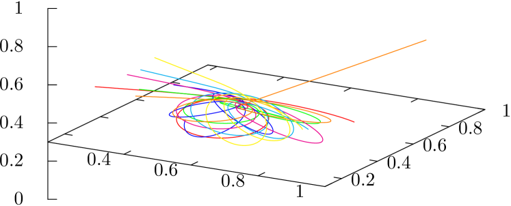
Fig. 3: Trajectory of seven out of 44 particles tracked to time $T=2$ with the fourth-order RK method and $\Delta t=.003$. The initial positions of the particles are visible on the left hand side.

The number of time steps required doubles with each refinement level. To allow for a meaningful comparison between different problem sizes, we measure the wall clock times for the RK method and all parallel algorithms in the final time step, averaging over the RK stages. We compute the per-tree element counts and the sparse forest at selected times of the simulation (see Figure 4), where we only use the timing of the last one at $T$.

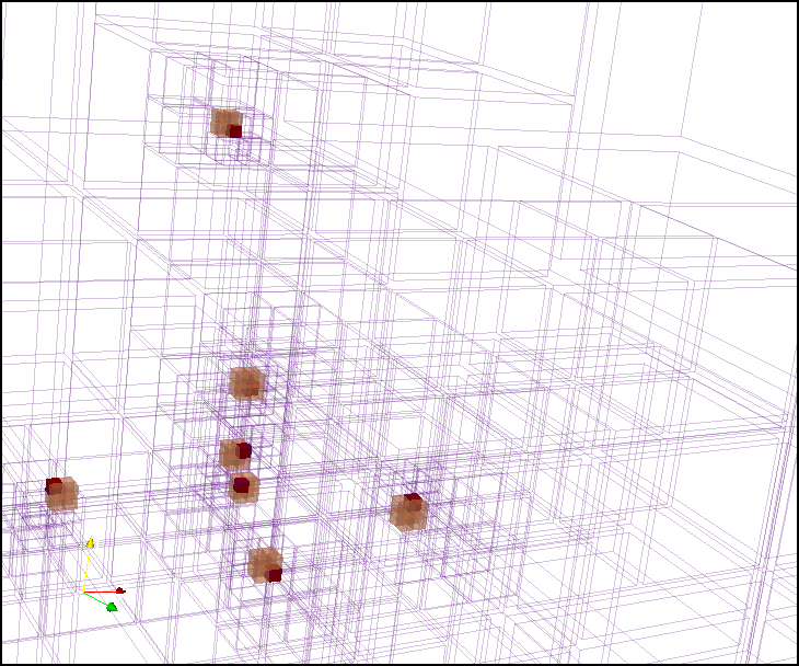
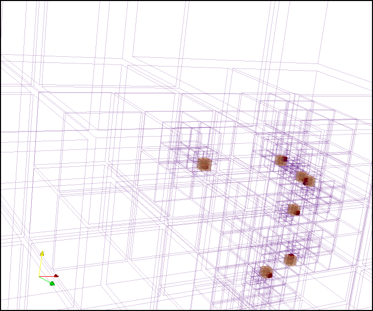
Fig. 4: Zoom into sparse forests created at time $t=0$ (left) and $t=.5$ (right), respectively, using the the same setup as for Figure 3, here with $\Delta t=.002$. Of the 44 particles tracked, the same seven are added to both sparse forests as individual level-8 elements (cf. Algorithm 6). Elements up to level 6 are drawn as blue wireframe, level 7 as transparent orange and level 8 as solid red.

We use three problem setups of increasing overall particle count and CFL, which we run to $T=.4$ with the 3rd order RK scheme (see Table 2). We use process counts from 16 to 65,536 in multiples of eight, which matches the multiplier of the particle counts and in consequence that of the element counts. The computations reported in this section have been run on Juqueen, an IBM BlueGene/Q system with 28 racks and a total of 28,672 16-core, 16 GB compute nodes (458,752 CPU cores) of type IBM PowerPC A2 (1.6 GHz) connected by a 5D-torus network with a dedicated collective subnet [40].

	particles			elements
levels	#req	#eff	#end	level	#eff	#end	$\Delta t$	#steps	#peers
3–9	12800	13318	12917	7	8548	12762	.008	50	5.31
5–11	819200	852580	842250	9	538392	784848	.002	200	6.96
7–13	52428800	54513360	54283090	11	34418420	49821220	.0005	800	7.12
3–9	102400	102374	98359	6	1632	2059	.016	25	8.06
5–11	6553600	6553472	6424887	8	102068	131587	.004	100	11.5
7–13	419430400	419415934	416393854	10	6530210	8700623	.001	400	11.1
4–10	5120000	5119830	4935040	8	55434	79486	.016	25	10.7
6–12	327680000	327677582	321323140	10	3528876	6366600	.004	100	22.6
8–14	20971520000	20971146506	20820237439	12	225760858	353507330	.001	400	19.7

Table 2: Three problem sizes, each run with process counts from 16 to 65,536 in multiples of 8. We only show every other run (multiple of 64). The problems have maximum particle counts per element $E$ of 5 and twice 320, respectively. For each run, we provide the specified minimum and maximum levels, the particle counts referring to the initial request, the count effectively reached on initialization, and the count at $T=.4$, respectively. Over time, we lose some particles that leave the domain. For the elements, we show the initial maximum level and global count and the count at final time $T$. Over time, we create more elements since they move closer together at $t=.4$, which leads to a deeper tree. On the right, we show the time step size, number of steps, and the average number of communication peers for particle transfer. The CFL number increases between the three problem sizes, which can bee seen by comparing the levels with $\Delta t$, and reflects in #peers. The overall largest run creates 20.97 billion particles.

6.2 Load balance

We know that p4est has a fast partitioning routine to equidistribute the elements between the processes [16]. Here we need to equidistribute the load of the RK time integration, which is proportional to the local number of particles. To this end, we assign each element a weight $w$ for partitioning that derives from the number of particles $e$ in this element, $w=1+e$. We offset the weight by 1 to bound the memory used by elements that contain zero or very few particles. We test the load balance by measuring the RK integration times in a weak and strong scaling experiment. From Figure 5 we see that scalability is indeed close to perfect.

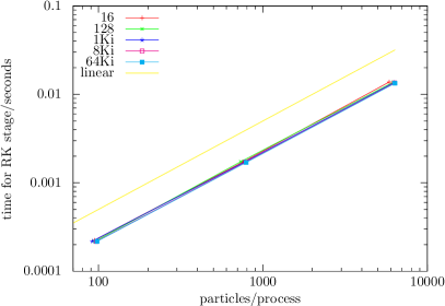
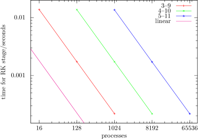
Fig. 5: Scaling of the Runge-Kutta time integration. We use the mid-size problem from Table 2 and rerun each line with $8\times$ and $64\times$ processes (equivalently, rerun the $8\times$ and $64\times$ smaller problems with the same process count), hence three dots per line. Left: The number of MPI processes is color-coded. We confirm optimal weak scaling since the dots lie on top of each other and optimal strong scaling by the fact that the lines lie on top of each other and have unit slope. Right: A typical strong scaling diagram, indicating simulation size by the levels of refinement. These plots indicate successful load balance by the particle-weighted partitioning of elements.

A weight function that counts both elements and particles in some ratio has been proposed before [26], as has the initialization of particles based on integrating a distribution function. In the above reference, parallelization is based on a one-element ghost layer. The use of algorithms like ours for non-local particle transfer and variable data, as we describe it below, has not yet been covered as far as we know.

6.3 Particle search and communication

We use the top-down forest traversal Algorithm 10, p4est_search_partition, augmented with a local search to determine for each local particle whether it changes the local element or leaves the process domain. In the first case, we find this element, and in the latter case, we find which process it is sent to. Once we know this, we reverse the communication pattern using sc_nary_notify to inform the receivers about the senders and send the particles using non-blocking MPI. We are not using one-sided MPI, since synchronization is often slower than messaging itself [27], which would defeat the purpose in our case.

Moving particles between elements is followed by mesh coarsening and refinement, which generally upsets the load balance, so we repartition the forest. This changes an individual element’s ownership, and thus the contained particles’ ownership, from one process to another. Thus, we transfer the particles a second time, now from the old to the new partition. We use the two-stage Algorithm 14, where we first send the number of particles for each element (fixed-size message volume per element) and then send the particles themselves (variable-size volume).

According to our measurements, sc_nary_notify has runtimes well below or around 1 ms for the small- and mid-size problems. The large problem gives rise to runtimes of about 5 ms. The fixed-size particle transfer is a sub-millisecond call.

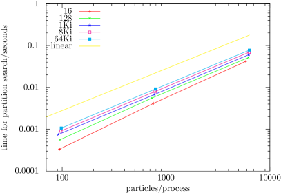
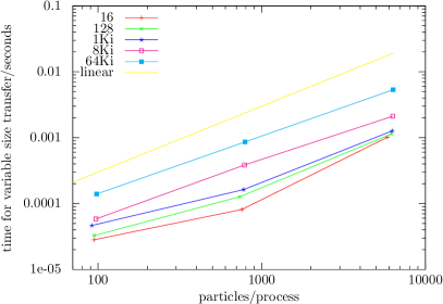
Fig. 6: Combined partition and local search (left) and transfer of variable-size element data (right) for the mid-size problem, where the runtimes are measured in the final time step.

Runtimes of the remaining calls p4est_search_partition and p4est_transfer_variable for the mid-size problem are displayed in Figure 6. Their scalability is generally acceptable given their small absolute runtimes.

$P$	small	medium	large
16	9.29e-3	41.9e-3	3.12
128	10.5e-3	51.6e-3	3.63
1024	11.6e-3	60.6e-3	4.13
8192	12.8e-3	69.4e-3	4.62
65536	13.9e-3	77.9e-3	5.10

$P$ / $K$	1	8	64	512
16	9.29e-3	9.05e-3	13.9e-3	58.4e-3
1024	11.6e-3	11.4e-3	16.3e-3	61.8e-3
65536	13.9e-3	13.7e-3	18.8e-3	66.2e-3

Table 3: Top: Absolute runtimes in seconds of p4est_search_partition augmented with a local search for the three problem sizes from Table 2. Each column presents a weak scaling exercise, where ideal times would be constant. The three runs have comparable rates between 60k and 82k particles per second. Bottom: We use a forest with $K$ trees in a cubic brick layout, where the refinement in each tree is reduced accordingly to make the meshes identical (shown for the small problem). For roughly a hundred trees and above the run times increase with $K$ while remaining largely independent of the process count $P$.

The runtimes of p4est_search_partition for all three problem sizes are compared in Table 3. They grow by less than a factor of 2 in weak scaling while increasing the process and particle counts by more than three orders of magnitude. In this test, we also experiment with forest meshes of up to $K=2^{d\times B}$ trees, where $B$ runs from 0 to 3 and per-tree minimum and maximum levels decrease by $B$, which keeps the meshes identical independent of $K$. Since the forest connectivity is unstructured, the limit of many trees loses the hierarchic property of the mesh, which reflects in a slower search. Up to 512 trees we see search times of less than 1/10th seconds for the small problem. For $1/8$th of the large problem (not shown in the table), the search times increase by a factor between 7 and 10 from 1 to 512 trees (.32 seconds on $K=1$, $P=16$ to 3.43 seconds on $K=512$, $P=64\mathrm{Ki}$).

6.4 Sparse forest and per-tree counts

At the end of the simulation, we create a sparse forest for output and post-processing. We use every 100th particle for the small size problem and every 1000th particle for the medium and large size problems; let us call this factor $R\geq 1$. The ratio of $E$ and $R$ and the specified maximum level determine the size of the sparse forest. If the maximum level is high, we create a deeper forest and more elements compared to the simulation. If $E/R$ is one, we keep the number of elements roughly the same, if it is less than one, the sparse forest will have less elements. These two effects may offset each other. In our examples, the sparse forest is smaller in the small-scale problem and larger in the mid- and large size problems. The build times of the largest run for each problem setup are 4.8 ms for the small, 20.5 ms for the medium, and 358 ms for the large size problem, each obtained with 65,536 MPI processes. Especially for the two larger problems, we have much less elements than particles, such that the number of elements per process is in the aggressive strong scaling regime.

The global per-tree counting of elements has runtimes below or around 1 ms except for the runs on 65,536 processes, where it is 4.4 ms for all three problem setups (using one tree). When reproducing the same mesh with a brick forest of as much as 512 trees, the run times do not change in any significant way. Since the messages are sent concurrently (the algorithm avoids daisy-chaining), this is achieved by design. This function has been tested in even more varied situations by the community for several years (transparently through p4est_save).

7 Demonstration: constructing random spheres

Particles, as considered in the previous demonstration, have extent zero and are only stored on one process at any given time. Now let us consider objects of non-trivial extent, for example geometric objects such as spheres. Depending on refinement and partition, and the individual spheres’ properties, some or even most spheres cover a region in space that is split between several processes. We require the global search proposed in Section 4, the variable-size data transfer from Section 5.2 and the pattern reversal from Section 5.3 to construct this model in parallel.

Our objective is to create multiple spheres based on a pseudorandom distribution and to refine the mesh at the spheres’ boundaries. The mesh refinement shall be reproducible and partition-independent. Such a setup may model a porous medium, where the spheres represent obstacles whose surface must be accurately resolved for a flow simulation in the empty space. Conversely, the spheres may be hollow and we increase their density to simulate percolation, treating the empty space as the solid matrix. Lastly, problems exist when only the surface of the spheres is of interest, for example in visualization applications [10].

7.1 Construction procedure

The construction has three parts. First, each process creates a certain number of spheres with centers inside its partition. For these spheres, the process becomes the current owner. Second, all remote processes intersecting an owned sphere’s surface are determined by the partition search, the spheres’ metadata is transferred to each such process, which we then use to decide where to refine the mesh. After refinement, we discard the copies. Third, we repartition the mesh, and the current owner of a sphere sends its metadata to its new owner. Steps two and three are repeated in a loop over increasing refinement levels to ensure that both the computational load and the memory consumption are well balanced.

We define a probability distribution of the spheres $\rho$ depending on their radius. To make all radii equally likely in a given volume, let

$$\rho(r)=c/r^{3},\quad r_{\mathrm{min}}\leq r\leq r_{\mathrm{max}},\quad\text{and $0$ otherwise}.$$ (16)

Normalization makes $c$ an expression in $r_{\mathrm{min}}$ and $r_{\mathrm{max}}$, and the expected volume is

$$V_{E}=\int_{r_{\mathrm{min}}}^{r_{\mathrm{max}}}\frac{4}{3}\pi r^{3}\rho(r)\mathrm{d}r=\frac{4}{3}\pi\frac{r_{\mathrm{min}}^{2}r_{\mathrm{max}}^{2}}{(r_{\mathrm{min}}+r_{\mathrm{max}})/2}=\frac{4}{3}\pi\frac{r_{\mathrm{geom}}^{4}}{r_{\mathrm{arith}}}.$$ (17)

To enforce an overall volume density $q$, an element of volume $V_{e}$ must have

$$N_{e}=qV_{e}/V_{E}$$ (18)

spheres on average, which we realize by sampling the number of constructed spheres separately for each element from a Poisson distribution with mean $N_{e}$. We sample the center coordinates of each sphere uniformly in the element and draw its radius from (16). This process is independent between elements, the only issue being the initialization of the random number generator in parallel. We resolve it by seeding the generator anew for each element with this elements’ lower left octree coordinates, which makes the distribution reproducible and partition-independent.

Fig. 7: Pseudo-random, reproducible, and partition-independent resolution of spheres (zoom into 2D example). On the left, we see the element intersecting the sphere’s center (red) and the refinement to its surface (green). On the right, we color by four MPI processes used and note that the refinement is non-local relative to the sphere’s owner quadrant and process. The refinement remains the same when using different numbers of processes (not shown). We do not enforce 2:1 balance; an element is refined if its parent intersected a sphere’s surface at some time during the refinement loop. See [10] for a continued discussion of this example in the context of in-situ visualization.

Figure 7 shows a typical construction along with the mesh.

7.2 Computational experiments

A scaling series can be devised by relating $r_{\mathrm{min}}$ and $r_{\mathrm{max}}$ to the minimal and maximal refinement levels and the MPI process count. If we divide both radii by two, the expected volume shrinks and the total number of spheres grows, each by a factor of eight in 3D. If, at the same time, we increase both minimal and maximal levels $\ell_{\mathrm{min}}$, $\ell_{\mathrm{max}}$ by 1, we achieve a constant ratio of spheres to elements. A weak scaling series emerges if we scale the number of processes by multiples of eight.

There is one parameter left to choose, namely the desired number of elements $s$ spanning a sphere’s radius. This parameter stops the refinement for larger spheres earlier than for smaller ones and ensures that the ratio of spheres to elements stays truly constant. We show some typical numbers for $s=4$ in Table 4 on up to 24,576 processes of the new Juwels supercomputer at JSC. We have used the “standard” compute nodes of Juwels, comprising dual Intel Xeon Platinum 8168 processors with 24 2.7 GHz cores each at 2 GB RAM per core, connected by EDR-Infiniband [18].

$P$	$\ell_{\mathrm{min}}$	$\ell_{\mathrm{max}}$	$r_{\mathrm{min}}$	$r_{\mathrm{max}}$	spheres	elements	$T_{\mathrm{pt}}$[s]	$T_{\mathrm{l}}$[s]
3,072	5	12	488u	63m	4.23M	1.50G	8m	20m
	6	13	244u	31m	33.8M	12.0G	40m	147m
24,576	7	14	122u	16m	271M	96.0G	47m	153m
	8	15	61u	7.8m	2.16G	768G†	$\ast$	$\ast$
	9	16	31u	3.9m	17.3G	$\ast$	$\ast$	$\ast$

Table 4: Scaling of 3D sphere sampling with $s=4$ elements per radius on the Juwels supercomputer. We use the size suffixes $u=10^{-6}$, $m=10^{-3}$, $M=10^{6}$, $G=10^{9}$. We observe that sphere and element counts scale by exact powers of eight, which confirms the validity of our pseudorandom generation for generating the spheres. The largest mesh refines to $768\times 10^{9}$ elements, where the symbol ${\dagger}$ indicates that subsequent partitioning exhausts the machine’s memory. At $\ell_{\mathrm{max}}=16$, we successfully create $17\times 10^{9}$ spheres but complete refinement only up to level 15. The rightmost two columns show the run times of partition search and variable-size transfer $T_{\mathrm{pt}}$ as introduced in this paper, and the run-time of the local search $T_{\mathrm{l}}$ for reference. We list the times in milliseconds, observing that the non-local algorithms require less than 1/20th of a second up to level 14.

8 Conclusion

This paper provides algorithms that support the efficient parallelization of computational applications of increased generality. Such generalization may refer to multiple aspects. One concerns the location of objects in the partition beyond a one-element ghost layer, together with flexible criteria for matching and pruning. Another is the fast repartitioning of variable-sized element data in linear storage. When considering the increased importance of scalable end-to-end simulation, our algorithms may aid in pre-processing (setting up correlated spatial fields in parallel, or finding physical source and receiver locations) and post-processing and reproducibility (writing/reading partition-independent formats of variable-size element data, optionally selecting readapted subsets).

Our algorithms are application-agnostic, that is, they do not interpret the data or meshes they handle, and perform well-defined tasks while hiding the complexity of their execution. Most are fairly low-level in the sense that they reside in the parallelization and metadata layer of an application. They can be integrated by third-party libraries and frameworks and often do not need to be exposed to the domain scientist. This approach supports modularity, code reuse, and ideally the division of responsibilities and quicker turnaround times in development.

We draw on the benefits of a distributed tree hierarchy and a linear ordering of mesh entities. Without such a hierarchy, the tasks we solve here would be a lot harder or even impractical (such as the partition search). We develop all algorithms for a multi-tree forest, noting that they apply meaningfully to the common special case of a single tree.

We find that any algorithm runtimes range between milliseconds and a few seconds, where one second or more occur only for specific algorithms using the largest setups. All algorithms are practical and scalable to 21e9 particles and 64Ki MPI processes on a BlueGene/Q supercomputer system. In addition, we verify the functionality on the newly installed Juwels system, creating up to 768e9 elements at a tree depth of 15 levels.

References

- [1] Mark James Abraham, Teemu Murtola, Roland Schulz, Szilárd Páll, Jeremy C. Smith, Berk Hess, and Erik Lindahl, GROMACS: High performance molecular simulations through multi-level parallelism from laptops to supercomputers, SoftwareX, 1-2 (2015), pp. 19–25.
- [2] M. Adams, P. Colella, D. T. Graves, J. N. Johnson, H. S. Johansen, N. D. Keen, T. J. Ligocki, D. F. Martin, P. W. McCorquodale, D. Modiano, P. O. Schwartz, T. D. Sternberg, and B. Van Straalen, Chombo software package for AMR applications – design document, tech. report, Lawrence Berkeley National Laboratory, 2015.
- [3] M. Ainsworth and J. T. Oden, A Posteriori Error Estimation in Finite Element Analysis, John Wiley & Sons, 2000.
- [4] Clelia Albrecht, Parallelization of adaptive gradient augmented level set methods, master’s thesis, Rheinische Friedrich-Wilhelms-Universität Bonn, 2016.
- [5] Utkarsh Ayachit, Andrew Bauer, Berk Geveci, Patrick O’Leary, Kenneth Moreland, Nathan Fabian, and Jeffrey Mauldin, ParaView Catalyst: Enabling in situ data analysis and visualization, in Proceedings of the First Workshop on In Situ Infrastructures for Enabling Extreme-Scale Analysis and Visualization, 2015, pp. 25–29.
- [6] I. Babuška and B. Q. Guo, The , and - version of the finite element method; basis theory and applications, Advances in Engineering Software, 15 (1992), pp. 159–174.
- [7] Michael Bader, Christian Böck, Johannes Schwaiger, and Csaba Vigh, Dynamically adaptive simulations with minimal memory requirement—solving the shallow water equations with Sierpinski curves, SIAM Journal of Scientific Computing, 32 (2010), pp. 212–228.
- [8] Wolfgang Bangerth, Ralf Hartmann, and Guido Kanschat, deal.II – a general-purpose object-oriented finite element library, ACM Transactions on Mathematical Software, 33 (2007), p. 24.
- [9] Carsten Burstedde, p4est: Parallel AMR on forests of octrees, 2010. http://www.p4est.org/ (last accessed June 3rd, 2019).
- [10] , Distributed-memory forest-of-octrees raycasting, 2018. http://arxiv.org/abs/1809.01334.
- [11] Carsten Burstedde, Martin Burtscher, Omar Ghattas, Georg Stadler, Tiankai Tu, and Lucas C. Wilcox, ALPS: A framework for parallel adaptive PDE solution, Journal of Physics: Conference Series, 180 (2009), p. 012009.
- [12] Carsten Burstedde, Omar Ghattas, Michael Gurnis, Tobin Isaac, Georg Stadler, Tim Warburton, and Lucas C. Wilcox, Extreme-scale AMR, in SC10: Proceedings of the International Conference for High Performance Computing, Networking, Storage and Analysis, ACM/IEEE, 2010.
- [13] Carsten Burstedde, Omar Ghattas, Georg Stadler, Tiankai Tu, and Lucas C. Wilcox, Towards adaptive mesh PDE simulations on petascale computers, in Proceedings of Teragrid ’08, 2008.
- [14] , Parallel scalable adjoint-based adaptive solution for variable-viscosity Stokes flows, Computer Methods in Applied Mechanics and Engineering, 198 (2009), pp. 1691–1700.
- [15] Carsten Burstedde and Johannes Holke, A tetrahedral space-filling curve for nonconforming adaptive meshes, SIAM Journal on Scientific Computing, 38 (2016), pp. C471–C503.
- [16] , p4est: Scalable algorithms for parallel adaptive mesh refinement, in JUQUEEN Extreme Scaling Workshop 2016, Dirk Brömmel, Wolfgang Frings, and Brian J. N. Wylie, eds., no. FZJ-JSC-IB-2016-01 in JSC Internal Report, Jülich Supercomputing Centre, 2016, pp. 49–54.
- [17] Carsten Burstedde, Lucas C. Wilcox, and Omar Ghattas, p4est: Scalable algorithms for parallel adaptive mesh refinement on forests of octrees, SIAM Journal on Scientific Computing, 33 (2011), pp. 1103–1133.
- [18] Jülich Supercomputing Center, Juwels configuration, 2019. Last accessed May 24th, 2019.
- [19] Bernardo Cockburn, George E. Karniadakis, and Chi-Wang Shu, Discontinuous Galerkin Methods: Theory, Computation and Applications, Lecture Notes in Computational Science and Engineering, Vol. 11, Springer, 2000.
- [20] John M. Dawson, Particle simulation of plasmas, Reviews of Modern Physics, 55 (1983).
- [21] John Drake, Ian Foster, John Michalakes, Brian Toonen, and Patrick Worley, Design and performance of a scalable parallel community climate model, Parallel Computing, 21 (1995), pp. 1571–1592.
- [22] A. Dubey, C. Daley, J. ZuHone, P. M. Ricker, K. Weide, and C. Graziani, Imposing a Lagrangian particle framework on an Eulerian hydrodynamics infrastructure in FLASH, The Astrophysical Journal Supplement Series, 201 (2012).
- [23] Wolfgang Eckhardt, Alexander Heinecke, Reinhold Bader, Matthias Brehm, Nicolay Hammer, Herbert Huber, Hans-Georg Kleinhenz, Jadran Vrabec, Hans Hasse, Martin Horsch, Martin Bernreuther, Colin W. Glass, Christoph Niethammer, Arndt Bode, and Hans-Joachim Bungartz, 591 TFLOPS multi-trillion particles simulation on SuperMUC, in ISC 2013, J. M. Kunkel, T. Ludwig, and H. W. Meuer, eds., vol. 7905 of Lecture Notes in Computer Science, Springer, 2013.
- [24] Paul F. Fischer, Gerald W. Kruse, and Francis Loth, Spectral element methods for transitional flows in complex geometries, Journal of Scientific Computing, 17 (2002), pp. 81–98.
- [25] James D. Foley, Andries van Dam, Steven K. Feiner, and John Hughes, Computer Graphics: Principles and Practice, Addison-Wesley, 2nd ed., 1990.
- [26] Rene Gassmoeller, Harsha Lokavarapu, Eric Heien, Elbridge Gerry Puckett, and Wolfgang Bangerth, Flexible and scalable particle-in-cell methods for geodynamic computations, Geochemistry, Geophysics, Geosystems, 19 (2018).
- [27] Robert Gerstenberger, Maciej Besta, and Torsten Hoefler, Enabling highly scalable remote memory access programming with MPI-3 one sided, Communications of the ACM, 61 (2018).
- [28] R. A. Gingold and J. J. Monaghan, Smoothed particle hydrodynamics: theory and application to non-spherical stars, Monthly Notes of the Royal Astronomical Society, 181 (1977), pp. 375–389.
- [29] Jens Glaser, Trung Dac Nguyen, Joshua A. Anderson, Pak Lui, Filippo Spiga, Jaime A. Millan, David C. Morse, and Sharon C. Glotzer, Strong scaling of general-purpose molecular dynamics simulations on GPUs, Computer Physics Communications, 192 (2015), pp. 97–107.
- [30] M. Griebel and G. W. Zumbusch, Parallel adaptive subspace correction schemes with applications to elasticity, Computer Methods in Applied Mechanics and Engineering, 184 (2000), pp. 303–332.
- [31] Arthur Guittet, Tobin Isaac, Carsten Burstedde, and Frédéric Gibou, Direct numerical simulation of incompressible flows on parallel octree grids. Submitted for publication, 2016.
- [32] Francis H. Harlow, The particle-in-cell computing method for fluid dynamics, Methods in Computational Physics, 3 (1964), pp. 319–343.
- [33] Francis H. Harlow and J. Eddie Welch, Numerical calculation of time-dependent viscous incompressible flow of fluid with free surface, Physics of Fluids, 8 (1965), pp. 2182–2189.
- [34] L. Hernquist and N. Katz, A unification of SPH with the hierarchical tree method, The Astrophysical Journal Supplement Series, 70 (1989), pp. 419–446.
- [35] D. Hilbert, Über die stetige Abbildung einer Linie auf ein Flächenstück, Mathematische Annalen, 38 (1891), pp. 459–460.
- [36] Torsten Hoefler, James Dinan, Rajeev Thakur, Brian Barrett, Pavan Balaji, William Gropp, and Keith Underwood, Remote memory access programming in MPI-3, ACM Transactions on Parallel Computing, 1 (2014).
- [37] C. Howlett, M. Manera, and W. J. Percival, L-PICOLA: A parallel code for fast dark matter simulation, Astronomy and Computing, 12 (2015), pp. 109–126.
- [38] Tobin Isaac, Carsten Burstedde, and Omar Ghattas, Low-cost parallel algorithms for 2:1 octree balance, in Proceedings of the 26th IEEE International Parallel & Distributed Processing Symposium, IEEE, 2012.
- [39] Tobin Isaac, Carsten Burstedde, Lucas C. Wilcox, and Omar Ghattas, Recursive algorithms for distributed forests of octrees, SIAM Journal on Scientific Computing, 37 (2015), pp. C497–C531.
- [40] Jülich Supercomputing Centre, JUQUEEN: IBM Blue Gene/Q supercomputer system at the Jülich Supercomputing Centre, Journal of large-scale research facilities, A1 (2015).
- [41] Randall J. LeVeque, Finite volume methods for hyperbolic problems, Cambridge University Press, 2002.
- [42] Shigang Li, Yenuan Zhang, and Torsten Hoefler, Cache-oblivious MPI all-to-all communications based on Morton order, IEEE Transactions on Parallel and Distributed Systems, 29 (2018).
- [43] Stephen L. W. McMillan and Sverre J. Aarseth, An integration scheme for collisional stellar systems, The Astrophysical Journal, 414 (1993), pp. 200–212.
- [44] Mohammad Mirzadeh, Arthur Guittet, Carsten Burstedde, and Frédéric Gibou, Parallel level-set methods on adaptive tree-based grids, Journal of Computational Physics, 322 (2016), pp. 345–364.
- [45] L. Moresi, F. Dufour, and H.-B. Mühlhaus, A Lagrangian integration point finite element method for large deformation modeling of viscoelastic geomaterials, Journal of Computational Physics, 184 (2003), pp. 476–497.
- [46] G. M. Morton, A computer oriented geodetic data base; and a new technique in file sequencing, tech. report, IBM Ltd., 1966.
- [47] Franco P. Preparata and Michael Shamos, Computational Geometry. An Introduction, Texts and Monographs in Computer Science, Springer, 1985.
- [48] Antonio Ragagnin, Nikola Tchipev, Michael Bader, Klaus Dolag, and Nicolay Hammer, Exploiting the space filling curve ordering of particles in the neighbour seach of Gadget3, in Parallel Computing: On the Road to Exascale, G. R. Joubert et.al., ed., IOS Press, 2016, pp. 411–420.
- [49] Abtin Rahimian, Ilya Lashuk, Shravan Veerapaneni, Aparna Chandramowlishwaran, Dhairya Malhotra, Logan Moon, Rahul Sampath, Aashay Shringarpure, Jeffrey Vetter, Richard Vuduc, et al., Petascale direct numerical simulation of blood flow on 200K cores and heterogeneous architectures, in Proceedings of the 2010 ACM/IEEE International Conference for High Performance Computing, Networking, Storage and Analysis, IEEE Computer Society, 2010, pp. 1–11.
- [50] Johann Rudi, A. Cristiano I. Malossi, Tobin Isaac, Georg Stadler, Michael Gurnis, Peter W. J. Staar, Yves Ineichen, Costas Bekas, Alessandro Curioni, and Omar Ghattas, An extreme-scale implicit solver for complex PDEs: highly heterogeneous flow in earth’s mantle, in Proceedings of the International Conference for High Performance Computing, Networking, Storage and Analysis, ACM, 2015, p. 5.
- [51] James R. Stewart and H. Carter Edwards, A framework approach for developing parallel adaptive multiphysics applications, Finite Elements in Analysis and Design, 40 (2004), pp. 1599–1617.
- [52] G. Strang and G. J. Fix, An Analysis of the Finite Element Method, Wellesley-Cambridge Press, 1988.
- [53] E. Suli, C. Schwab, and P. Houston, -DGFEM for partial differential equations with nonnegative characteristic form, in Discontinuous Galerkin Methods. Theory, Computation and Applications, B. Cockburn, G. E. Karniadakis, and C. W. Shu, eds., Lecture Notes in Computational Science and Engineering, Springer, 2000, pp. 221–230.
- [54] Hari Sundar, George Biros, Carsten Burstedde, Johann Rudi, Omar Ghattas, and Georg Stadler, Parallel geometric-algebraic multigrid on unstructured forests of octrees, in SC12: Proceedings of the International Conference for High Performance Computing, Networking, Storage and Analysis, Salt Lake City, UT, 2012, ACM/IEEE.
- [55] Hari Sundar, Rahul Sampath, and George Biros, Bottom-up construction and 2:1 balance refinement of linear octrees in parallel, SIAM Journal on Scientific Computing, 30 (2008), pp. 2675–2708.
- [56] Tiankai Tu, David R. O’Hallaron, and Omar Ghattas, Scalable parallel octree meshing for terascale applications, in SC ’05: Proceedings of the International Conference for High Performance Computing, Networking, Storage, and Analysis, ACM/IEEE, 2005.
- [57] Dong Wang, Yisong Zhou, and Sihong Shao, Efficient implementation of smoothed particle hydrodynamics (SPH) with plane sweep algorithm, Communications in Computational Physics, 19 (2016), pp. 770–800.