Calibrating Model-Based Inferences and Decisions

Abstract

As the frontiers of applied statistics progress through increasingly complex experiments we must exploit increasingly sophisticated inferential models to analyze the observations we make. In order to avoid misleading or outright erroneous inferences we then have to be increasingly diligent in scrutinizing the consequences of those modeling assumptions. Fortunately model-based methods of statistical inference naturally define procedures for quantifying the scope of inferential outcomes and calibrating corresponding decision making processes. In this paper I review the construction and implementation of the particular procedures that arise within frequentist and Bayesian methodologies.

As observations and experiments become more sophisticated, and we ask correspondingly more detailed questions about the world around us, we must consider increasingly more complex inferential models. The more complex the model, however, the more subtle the corresponding inferences, and the decisions informed by those inferences, will behave.

Consequently understanding how inferences and decisions vary across the the many possible realizations of a measurement becomes a critical aspect in the design and preliminary evaluation of new observational efforts. Such sensitivity analyses have a long history in the applied sciences but they are often built upon heuristics. Fortunately, formal methods of statistical inference naturally admit procedures for understanding and then calibrating the inferential consequences of measurements within the scope of a statistical model. The exact mathematical construction of this calibration, and the crucial implementation details, depend critically on the exact form on inference that we consider.

In this paper I review how inferential outcomes are formally calibrated within both the frequentist and Bayesian perspectives. I discuss not only the procedures but also the conceptual and practical challenges in implementing these procedures in practice, and demonstrate their application towards calibrating traditional discovery and limit setting results.

1 Mathematical Preliminaries

In order to be as explicit as possible when introducing new functions I will use the conventional mathematical notation. A function, $f$, that maps points $x$ in a space $X$ to points $y=f(x)$ in a space $Y$ is denoted

$$f:\; X \rightarrow Y$$

$$x \mapsto f(x)$$ .

The real number line will be denoted $\mathbb{R}$ with the $N$-dimensional real numbers denoted $\mathbb{R}^{N}$.

Sets of objects are denoted with curly braces, $\{\ldots\}$, and a vertical line in between braces denotes a selection condition which defines a set. For example,

$$\{x\in X\mid f(x)=0\}$$

defines the subset of points in $X$ that satisfies the condition $f(x)=0$.

Finally,

$$x\sim\pi(x)$$

implies that the space $X\ni x$ is endowed with the probability distribution, $\pi$. If the left-hand side is decorated with a tilde,

$$\tilde{x}\sim\pi(x)$$

then this implies that $\tilde{x}$ is a sample from the probability distribution $\pi$.

2 Inference

Ultimately statistics is a tool to learn about the phenomenological behavior of some latent system, for example the internal structure and dynamics of a subatomic particle, the phenotypical encoding of a genome, or the response of a population of individuals to a particular stimulus. Although we cannot observe these phenomena directly we can probe them through measurements of the system, or more precisely measurements of how the system interacts with a surrounding environment. These experimental probes can be passive, assembling and analyzing data collected for other purposes, or active, collecting data from dedicated experiments.

Formally any measurement process defines a measurement space, $Y$, containing all of the possible realizations of a measurement. These realizations, or observations are inherently stochastic, varying from measurement to measurement. If we assume that this variation is sufficiently well-behaved, then we can mathematically quantify it with a probability distribution over $Y$. I will refer to any probability distribution over the measurement space as a data generating process. Under this assumption observations of a given system are modeled as independent samples from some true data generating process, $\pi^{*}$.

Inference is any procedure that uses observations to inform our understanding of the latent system and its behaviors (Figure 1). Because of the inherent stochasticity of the measurement process, however, any finite observation will convey only limited information. Consequently inference fundamentally concerns itself with quantifying the uncertainty in this understanding.

Figure 1: Inference is an inductive process that aims to quantify which phenomenological behaviors of a latent system are consistent with measured observations. Formally we assume that the measurement process defines a space of observations, $Y$, and a probability distribution quantifying the variation in those observations, $\pi^{*}$. Any realization of the measurement process results in an observation, $\tilde{y}$, from which we base our inferences about the latent system and any resulting decisions about how to interact with the latent system.

In particular, there will be many phenomenological behaviors consistent with a given observation and, in general, those behaviors that appear most consistent will vary along with the form of the observation itself. Here I will define the sensitivity of an experiment as the distribution of inferential outcomes induced by the variation in the observations. Ideally our inferences would be accurate and capture the true behavior of the latent system regardless of the details of particular observation, but there are no generic guarantees. Consequently in practice we must be careful to study these sensitivities with respect to our inferential goals.

Sensitivity analyses become even more important when we consider decisions informed by our inferences. Conventions in many fields focus not on reporting uncertainties but rather making explicit claims about the latent system being studied. These claims commonly take the form of discovery, where a particular phenomenon is claimed to exist or not exist. In order to limit the possibility that we falsely claim to have discovered the presence, or absence, of a phenomenon we have to carefully consider the sensitivity of these claims.

Decisions, however, are not always so obvious. Even the simple presentation of our inferences requires implicit decisions in the form of how we summarize and communicate our results. To ensure that we are not biasing our audience or ourselves we have to consider how this presentation would vary with the underlying observations.

Ultimately, in order to ensure robust analyses we have to carefully calibrate the consequences of our inferences. First consider a set of actions that we can take, $a\in A$. Assuming a perfect characterization of the latent system of interest we could theoretically quantify the relative loss of taking a given action with the true loss function,

$$L^{*}: \,A\rightarrow\mathbb{R}$$

$$\,\,a\,\mapsto L^{*}(a).$$

If we convolving this loss function with an inferential decision-making process that maps observations to actions,

$$\hat{a}: \,Y\rightarrow A$$

$$\,y\,\,\mapsto\hat{a}(y),$$

we induces a true inferential loss function,

$$L^{*}_{\hat{a}}: \,Y\rightarrow\mathbb{R}$$

$$\,y\,\,\mapsto L^{*}(\hat{a}(y)).$$

More optimistic readers might also consider the equivalent utility function, $U^{*}(a)\equiv-L^{*}(a)$.

A sensitivity analysis considers the distribution of $L^{*}_{\hat{a}}(y)$ with varying observations, $y$, while a calibration considers expected values of the loss function over the possible observations. For example, we might aim to calibrate an experiment to ensure that the average loss is below a certain value or that a particular quantile of the loss distribution is below a certain value.

These analyses, however, require that we know both the true behavior of the latent system, so that we can quantify the relative loss of each action, and the true data generating process, so that we can quantify the variation of possible observations. In practice we don’t know the true nature of the latent system or the true data generating process of the resulting measurements, but we can model them. Statistical models quantify the scope of possible data generating processes, allowing us to quantify the sensitivity of inferences and then construct formal calibrations within that scope.

3 Model-Based Sensitivities and Calibration

Inferences that explicitly model the measurement process, or model-based inferences, naturally define the scope of the possible observations, leaving practitioners to employ their domain expertise to construct relevant loss functions.

In this section I review the model configuration space that underlies model-based inference and how the frequentist and Bayesian paradigms utilize this space to define inference and calibrate inferential outcomes.

3.1 The Model Configuration Space

A statistical model establishes a model configuration space, or a collection of data generating processes. Ideally the model configuration space is designed to be sufficiently rich to either contain the true data generating process or, more realistically, contain data generating processes sufficiently similar to the true data generating process within the resolution of our experimental probe (Figure 2). Each individual data generating process in the model configuration space will be denoted a model configuration.

Figure 2: (a) The true data generating process, $\pi^{*}$, belongs in the space of all possible data generating processes over the measurement space, $\mathcal{P}_{Y}$. (b) Model-based inferences consider a model configuration space, $\mathcal{M}$, which contains only a limited subset of all of those possible data generating processes.

Typically the model configuration space admits a parameterization in which each model configuration can be identified with a parameter value, $\theta\in\Theta$. Often these parameters decompose into components,

$$\theta=\left\{\theta_{1},\ldots,\theta_{N}\right\}$$

with each component responsible for quantifying only one aspect of the phenomenological behavior of the latent system, the environment containing the latent system, or the measurement process itself. Such parameter decompositions make the model configuration space particularly interpretable.

Moreover, if each model configuration admits a density with respect to a common reference measure over $Y$ then we can fully specify the model configuration space with the family of densities $\pi(y\mid\theta)$ for $y\in Y$ and $\theta\in\Theta$. In many applied fields this family of densities, or even the model configuration space itself, is introduced as the likelihood. Unfortunately, that term has a more precise definition in the statistics literature: the phrase likelihood is used exclusively to denote the function over the parameter space given by evaluating each density at a particular measurement $\tilde{y}\in Y$,

$$\mathcal{L}_{\tilde{y}} :\Theta\rightarrow\mathbb{R}$$

$$\quad\theta\,\mapsto\pi(\tilde{y}\mid\theta).$$

Consequently I will avoid the use of likelihood unless the model configuration densities are explicitly being evaluated at a given observation.

Once we have constructed a model configuration space, inference becomes a means of identifying those model configurations that are consistent with an observation (Figure 3). Because there is no unique definition of this sort of consistency, there are multiple approaches to inference. The two employed most in practice are frequentist and Bayesian inference.

Figure 3: In model based inference the measurement process is modeled with a model configuration space, $\Theta$. Inferences identify which model configurations, $\theta\in\Theta$, are consistent with a given observation, which then informs the properties of the true data generating process and the latent system under investigation.

3.2 Model-Based Loss Functions

Given a means of quantifying those model configurations consistent with an observation, we can use that quantification to motivate fruitful decisions about how to best interact with the latent system. For example we may want to intervene with the system or systems like it, introducing a treatment or altering the surrounding environment. Alternatively we may want to decide on whether or not to claim the discovery of the absence or presence of a new phenomenon, or whether or not to follow up with another experiment.

For model-based inference we can quantify the utility of a set of actions by defining a loss function for each possible data generating process in our model,

$$L: \,A\times\Theta\rightarrow\mathbb{R}$$

$$\,\,\,(a,\theta)\,\,\mapsto L(a,\theta).$$

Given an inferential decision making process

$$\hat{a}: \,Y\rightarrow A$$

$$\,y\,\,\mapsto\hat{a}(y),$$

we can then define a model-based inferential loss function,

$$L_{\hat{a}}: \,Y\times\Theta\rightarrow\mathbb{R}$$

$$\,\,\,(y,\theta)\,\,\mapsto L(\hat{a}(y),\theta).$$

Presuming that the true data generating process is contained within the model configuration space, sensitivity analyses and calibration within the scope of our model quantifies the actual performance of our decisions. When the true data generating process is close to the model configuration space then this process approximates the actual performance.

That said, constructing a loss function alone is insufficient to admit sensitivity analyses and calibrations. Before the measurement we are ignorant of not only what the observation will be, and hence what action we will take, but also which model configuration gives the true data generating process. In order to quantify the performance of our decisions we have to define the scope of possible observations and possible data generating processes. Exactly how we do that depends intimately on the formal details of the inferences that we make.

3.3 Sensitivity and Calibration of Frequentist Inference

Frequentist inference (Casella and Berger, 2002; Lehmann and Casella, 2006; Keener, 2011) derives from the interpretation that probability theory can model only the frequencies of repeatable processes. This definition is consistent with the use of probabilities to model the inherent variation of observations, but it does not allow us to define probabilities over the model configuration space itself, as those probabilities would not correspond to the hypothetical frequencies of any repeatable process. Ultimately this strong philosophical assumption implies that we cannot use any form of weighting to quantify consistency in the model configuration space because any self-consistent weighting is equivalent to the assignment of probabilities!

Consequently frequentist inference must take the form of definite decisions about which parts of the model configuration space are consistent with an observation and which are not. From a frequentist perspective inference and decisions are one in the same! Because such definite decisions can readily exclude the true data generating process, or model configurations close to the true data generating process, from consideration we have to carefully calibrate these decisions so that such exclusions are sufficiently rare.

Ultimately frequentist inference does not define exactly how an observation informs which parts of the model configuration space to keep and which to discard. Rather frequentist inference establishes a means of calibrating any such procedure that might be considered.

3.3.1 Frequentist Inference

Any procedure that consumes an observation to produce a definite decision about which parts of the model configuration space are considered consistent takes the mathematical form of an estimator. Estimators are functions from the measurement space to subsets of the model configuration space, mapping observations to subsets of model configurations,

$$\hat{\theta}:Y\rightarrow\mathcal{T},$$

where $\mathcal{T}$ is the space of well-defined subsets of the model configuration space, $\Theta$.

A common class of estimators are point estimators that identify a single point in the model configuration space (Figure 4a),

$$\hat{\theta}:Y\rightarrow\Theta,$$

Point estimators formalize the intuition of a “best fit”, where inferences are summarized with a single point at the expense of ignoring the uncertainty inherent in learning from finite observations.

The more general class of estimators that identify entire subsets of the model configuration space are known as confidence sets (Figure 4b), or confidence intervals if the model configuration space is one-dimensional. The nomenclature is meant to suggest that if a confidence set has been properly constructed then we can be confident that these sets will contain the true data generating process for sufficiently many observations.

Figure 4: (a) Point estimators identify a single model configuration, $\hat{\theta}(\tilde{y})$, that is ideally close to the true data generating process, $\theta^{*}$, for any given observation $\tilde{y}$. (b) Confidence sets identify entire subsets of the model configuration space that ideally contain the true data generating process for any given observation.

3.3.2 The Frequentist Calibration Criterion

The actual choice of which estimator to employ in a given analysis is left to the practitioner. Constraints that enforce desired properties can be imposed to restrict the space of potential estimators, but the choice of these desired properties remains the responsibility of the practitioner. Regardless of how we ultimately select an estimator, however, we can use the model configuration space to calibrate the estimator and determine it’s practical utility.

In frequentist inference our actions are definite quantifications of the model configuration space and, by construction, estimators are inferential decision making processes. In order to define a calibration criterion we we must first construct a model-based loss function,

$$L(\hat{\theta},\theta),$$

that quantifies how well $\hat{\theta}$ identifies the true data generating process, $\theta$. Substituting an estimator yields the model-based inferential loss function,

$$L_{\hat{\theta}}(y,\theta)\equiv L(\hat{\theta}(y),\theta).$$

As with estimators there is no canonical loss function in frequentist inference; instead one must be chosen using whatever domain expertise is available within the context of a particular analysis. In practice this choice often considers the structure of the estimator itself.

If we knew that a given $\theta$ identified the true data generating process then the sensitivity of the loss of the estimator over the possible observations could be summarized with an expectation over that configuration. This expectation yields an expected loss for each model configuration,

$$L_{\hat{\theta}}(\theta)=\int_{Y}\mathrm{d}y\,\pi(y\mid\theta)\,L_{\hat{\theta}}(y,\theta).$$

Because we don’t have any information about which model configuration identifies the true data generating process before a measurement is made, the frequentist calibration criterion is defined as the maximum expected loss over all possible model configurations,

$$\bar{L}_{\hat{\theta}}=\max_{\theta}L_{\hat{\theta}}(\theta).$$

If the model configuration space is sufficiently rich that it contains the true data generating process, then this calibration criterion defines the worst case loss of our given estimator. Bounding the worst case loss of an estimator is an extremely powerful guarantee on its practical performance, but also a very conservative one as bounds can be dominated by unrealistic but not impossible data generating processes towards the boundaries of the model configuration space.

A natural loss function for point estimators is the $L^{p}$ distance between the estimated model configuration and the presumed true data generating process,

$$L^{p}_{\hat{\theta}}(y,\theta)=((\theta-\hat{\theta}(y))^{2})^{p/2}.$$

The expected $L^{p=2}$ loss is known as the variance of an estimator.

Similarly, a natural natural loss function for confidence sets is inclusion of the presumed true data generating process,

$$L_{\hat{\theta}}(y,\theta)=\mathbb{I}_{\theta}[\hat{\theta}(y)],$$

where the indicator function, $\mathbb{I}$, is defined as

$$\mathbb{I}_{\theta}[T]=\left\{\begin{array}[]{rc}1,&\theta\in T\\ 0,&\mathrm{else}\end{array}\right..$$

The expected inclusion loss, or coverage is simply how often the confidence set contains the presumed true data generating process.

While this calibration procedure can used to analyze the frequentist properties of a given estimator, they can also be used to optimize the choice of estimator. Given a family of estimators, $\{\hat{\theta}_{x}\}$, the optimal estimator will satisfy the minimax criterion,

$$\hat{\theta}^{*} =\underset{x}{\mathrm{argmin}}\,L_{\hat{\theta}_{x}}^{*}$$

$$=\underset{x}{\mathrm{argmin}}\max_{\theta}\,L_{\hat{\theta}_{x}}(\theta)$$

$$=\underset{x}{\mathrm{argmin}}\max_{\theta}\,\int_{Y}\mathrm{d}y\,\pi(y\mid\theta)\,L_{\hat{\theta}_{x}}(y,\theta).$$

For example, a desired coverage might be established initially and then a confidence set engineered to ensure that the coverage is met, or exceeded, for all of the data generating processes in the model configuration space.

3.3.3 Frequentist Methods in Practice

Aside from the conceptual challenge of choosing a loss function that enforces the needs of a given analysis, the computational burden of frequentist calibration is a significant impediment to its application. In particular, even approximately scanning through the model configuration space to identify the maximal expected loss often requires more computational resources than realistically available to a practitioner.

Many frequentist analyses assume sufficiently simple model configuration spaces, estimators, and loss functions such that the maximum expected loss can be computed analytically. The analytic results allow, for example, optimal estimators to be chosen from families of candidate estimators with strong guarantees on the performance of the best choice. The practical validity of these guarantees, however, requires that the true data generating process be simple enough that it can be contained within the relatively crude model configuration space. For the complex experiments of applied interest this can be a dangerous assumption.

Without analytic results one might consider interpolative methods that bound the variation in the expected loss between a grid of points distributed across the model configuration space. At each of these points Monte Carlo methods can be used to simulate observations and approximate the expected loss, and then the properties of the loss function itself can be used to interpolate the expected loss amidst the grid points. These methods can yield reasonable results for low-dimensional model configuration spaces, but as the dimensionality of the model increases even strong smoothness assumptions can become insufficient to inform how to interpolate between the grid points.

In order to avoid this curse of dimensionality frequentist analyses unaccommodating to analytic results often resort to asymptotics. Asymptotic analyses assume that the model configuration space is sufficiently regular that as we consider more observations at once the behavior of the model configuration space follows a central limit theorem. Under these conditions the likelihood for any observation concentrates in an increasingly small neighborhood around the maximum likelihood estimator,

$$\theta_{\mathrm{ML}}(y)=\underset{\theta\in\Theta}{\mathrm{argmax}}\,\pi(\tilde{y}\mid\theta).$$

Moreover, in this limit the breadth of that neighborhood is given by the inverse of the Fisher information matrix,

$$I(\tilde{y})=\left.\nabla^{2}\pi(\tilde{y}\mid\theta)\right|_{\theta=\theta_{\mathrm{ML}}(y)}.$$

The concentration in the model configuration space in this asymptotic limit admits convenient analytic approximations to the frequentist calibration procedure.

Asymptotic behavior also motivates the concept of profiling, which is of use when the parameter space separates into phenomenological parameters related to the underlying system of interest and nuisance or systematic parameters that are unrelated to that system but still effect the data generating process. Under certain conditions the observations inform the nuisance parameters faster than the the phenomenological parameters; in the asymptotic limit the uncertainty in these parameters becomes negligible and they can be replaced with conditional maximum likelihood estimates.

More formally, if the parameterization of the model configuration space decomposes into phenomenological parameters, $\vartheta$, and nuisance parameters, $\sigma$, then we define the conditional maximum likelihood estimator as

$$\hat{\sigma}(\vartheta,\tilde{y})=\underset{\sigma}{\mathrm{argmax}}\,\pi(\tilde{y}\mid\vartheta,\sigma)$$

and the corresponding profile likelihood as

$$\hat{\pi}(\tilde{y}\mid\vartheta)=\pi(\tilde{y}\mid\vartheta,\hat{\sigma}(\vartheta,\tilde{y})).$$

The profile likelihood can then be used to calibrate estimators of the phenomenological parameters, at least in this limit.

The utility of these asymptotic methods depends critically on the structure of the model configuration space and its behavior as we consider more observations. Simpler models typically converge to the asymptotic limit faster and hence require fewer data for asymptotic calibrations to be reasonably accurate. More complex models, however, converge more slowly and may require more data than is practical, or they may not satisfy the necessary conditions to converge at all.

Consequently it is crucial to explicitly verify that the asymptotic regime has been reached in a given analysis. As with analytic methods, one has to be especially careful to not employ an over-simplistic model to facilitate the applicability of the asymptotic results while compromising the practical validity of the resulting calibration.

3.4 Sensitivity and Calibration of Bayesian Inference

Bayesian inference (Bernardo and Smith, 2009; Gelman et al., 2014) broadens the interpretation of probability theory, allowing it to be used to not only model inherent variation in observations but also provide a probabilistic quantification of consistency between the data generating processes in the model configuration space and observations.

This generalization manifests in a unique procedure for constructing inferences which can then be used to inform decisions. Ultimately Bayesian inference decouples inference from decision making, making the assumptions underlying both more explicit and often easier to communicate. Moreover, the fully probabilistic treatment of the Bayesian perspective immediate defines a procedure for constructing sensitivities and calibrations.

3.4.1 Bayesian Inference

Bayesian inference compliments the data generating processes in the model configuration space with a prior distribution over the model configuration space itself. The prior distribution quantifies any information on which model configurations are closer to the true data generating process than others that is available before a measurement is made. This information can come from, for example, physical considerations, previous experiments, or even expert elicitation. Careful choices of the prior distribution can go a long way towards regularizing unwelcome behavior of the model configuration space.

Together the model configuration space and the prior distribution define the Bayesian joint distribution over the measurement space and the parameter space,

$$\pi(y,\theta)=\pi(y\mid\theta)\pi(\theta).$$

The titular Bayes’ Theorem conditions this joint distribution on an observation, $\tilde{y}$, to give the posterior distribution,

$$\pi(\theta\mid\tilde{y})=\frac{\pi(\tilde{y},\theta)}{\pi(\tilde{y})}\propto\pi(\tilde{y}\mid\theta)\,\pi(\theta).$$

In words, the prior distribution quantifies information available before the measurement, the model configuration space decodes the information within an observations, and the posterior distribution combines both sources of information to quantify the information about the latent system being studies after a measurement (Figure 5).

Figure 5: (a) Bayesian inference begins with a prior distribution, shown here in dark red, over the model configuration space, $\mathcal{M}$, that quantifies information available before a measurement. (b) Information encoded in an observation updates the prior distribution into a posterior distribution that ideally concentrates around the true data generating process, $\pi^{*}$.

Any well-posed statistical query we might make of our system reduces to interrogations of the posterior distribution. Mathematically this must take the form of a posterior expectation for some function, $f$,

$$\mathbb{E}[f]=\int_{\Theta}\mathrm{d}\theta\,\pi(\theta\mid\tilde{y})\,f(\theta).$$

For example, we might consider the posterior mean or median to identify where the posterior is concentrating or the posterior standard deviation or the posterior quartiles to quantify the breadth of the distribution.

Posterior expectations also define a unique decision making process in Bayesian inference. First we define the expected loss for a given action by averaging a model-based loss function, $L(a,\theta)$, over the posterior distribution,

$$L(a,\tilde{y})=\int_{\Theta}\mathrm{d}\theta\,\pi(\theta\mid\tilde{y})L(a,\theta).$$

We can then define a decision making process by taking the action with the smallest expected loss,

$$a^{*}(\tilde{y})=\min_{a\in A}L(a,\tilde{y}).$$

For example, our decision might be to summarize the posterior with a single “best fit” model configuration, $\hat{\theta}$. Given the loss function

$$L(\hat{\theta},\theta)=(\hat{\theta}-\theta)^{2}$$

the expected losses for each possible summary becomes

$$L(\hat{\theta},\tilde{y})=(\hat{\theta}-\mu(\tilde{y}))+\sigma^{2}(\tilde{y}),$$

where $\mu(\tilde{y})$ is the posterior mean and $\sigma(\tilde{y})$ is the posterior standard deviation. Following the Bayesian decision making process, our optimal decision is to summarize our posterior by reporting the posterior mean, $\hat{\theta}^{*}(\tilde{y})=\mu(\tilde{y})$.

3.4.2 The Bayesian Calibration Criterion

Bayes’ Theorem provides a unique procedure for constructing inferences and making subsequent decisions given an observation, but there are no guarantees that these decisions will achieve any desired performance for any possible observation. Consequently sensitivity analysis and calibration of this decision making process across possible is still important in Bayesian inference.

Instead of having to consider each model configuration equally, however, the prior distribution allows us to diminish the effect of unrealistic but not impossible model configurations. In particular sampling from the joint distribution generates an ensemble of reasonable data generating process and corresponding observations which we can use to quantify the performance of our decisions.

For example, we can quantify the sensitivity of any inferential outcome by integrating the model configurations out of the Bayesian joint to give the prior data generating process,

$$\pi(y)=\int_{\Theta}\mathrm{d}\theta\,\pi(y,\theta)=\int_{\Theta}\mathrm{d}\theta\,\pi(y\mid\theta)\,\pi(\theta).$$

The prior data generating process probabilistically aggregates the behaviors of all of the possible data generating process in the model configuration space into a single probability distribution over the measurement space. We can then analyze the sensitivity of any inferential outcome by running our analysis over an ensemble of observations sampled from this distribution.

Moreover, we can calibrate a decision making process by integrating a model-based loss function against the full Bayesian joint distribution,

$$\bar{L}_{A}=\int_{Y,\Theta}\mathrm{d}y\,\mathrm{d}\theta\,L_{\hat{a}}(y,\theta)\pi(\theta,y).$$

This calibration immediately quantifies the expected loss as both the observations and data generating processes vary within the scope of our model.

3.4.3 Bayesian Methods in Practice

The unified probabilistic treatment of Bayesian inference ensures that all calculations take the form of expectation values with respect the Bayesian joint distribution, its marginals, such as the prior distribution and the prior data generating process, or its conditionals, such as the posterior distribution. Consequently calculating expectation values, or more realistically accurately estimating them, is the sole computational burden of Bayesian inference.

Posterior expectations are challenging to compute, and indeed much of the effort on the frontiers of statistical research concerns the development and understanding of approximation methods. One of the most powerful and well-understood of these is Markov chain Monte Carlo (Robert and Casella, 1999; Brooks et al., 2011) and its state of the art implementations like Hamiltonian Monte Carlo (Betancourt, 2017).

On the other hand, expectations with respect to the Bayesian joint distribution are often amenable to much simpler Monte Carlo methods. In particular, if we can draw exact samples from the prior distribution and each of the data generating processes in the model configuration space then we can generate joint samples with the sequential sampling scheme

$$\tilde{\theta} \sim\pi(\theta)$$

$$\tilde{y} \sim\pi(y\mid\tilde{\theta}).$$

For each simulated observation, $\tilde{y}$, we can construct a subsequent posterior distribution, make posterior-informed decisions, and then compare those decisions to the simulated truth, $\tilde{\theta}$. As we generate a larger sample from the Bayesian joint distribution we can more accurately quantify our sensitivities and calibrations.

We can also quantify how sensitivity a calibration is to a particular component of the parameter space, $\vartheta$, by sampling the complementary parameters, $\sigma$, from the corresponding conditional prior distribution,

$$\tilde{\sigma} \sim\pi(\sigma\mid\vartheta)$$

$$\tilde{y} \sim\pi(y\mid(\vartheta,\tilde{\sigma})).$$

This allows us, for example, to see how our decision making process behaves as for various phenomenlogical behaviors.

Interestingly, the application of Monte Carlo to the Bayesian joint distribution is not at all dissimilar to many of the heuristic schemes common in the sciences. Sampling $\tilde{y}\sim\pi(y\mid\tilde{\theta})$ just simulates the experiment conditioned on the model configuration, $\tilde{\theta}$. The addition step $\theta\sim\pi(\theta)$ simply simulates model configurations consistent with the given prior information instead of selecting a few model configuration by hand.

One inferential outcome immediately amenable to calibration is the approximation of posterior expectations themselves. Cook, Gelman and Rubin (2006), for example, introduce a natural way to calibrate the estimation of any posterior quantiles. This then immediately provides a procedure for quantifying the accuracy of any algorithm that yields deterministic approximations to posterior quantiles, for example as demonstrated in Yao et al. (2018).

Bayesian sensitivity analysis is particularly useful for identifying known pathologies in Bayesian inference by carefully examining the simulated analyses. Consider, for example, the posterior $z$-score for the parameter component, $\tilde{\theta}_{n}$,

$$z_{n}=\left|\frac{\mu_{n}(\tilde{y})-\tilde{\theta}_{n}}{\sigma_{n}(\tilde{y})}\right|,$$

where $\mu_{n}(\tilde{y})$ denotes the posterior mean of $\tilde{\theta}_{n}$ and $\sigma_{n}(\tilde{y})$ the corresponding posterior standard deviation. The posterior $z$-score quantifies how much the posterior distribution envelops the presumed true data generating process along this direction in parameter space. At the same time consider the posterior shrinkage of that parameter component,

$$s_{n}=1-\frac{\sigma_{n}^{2}(\tilde{y})}{\tau_{n}^{2}(\tilde{y})},$$

were $\tau_{n}(\tilde{y})$ is the prior standard deviation of $\tilde{\theta}_{n}$. The posterior shrinkage quantifies how much the posterior distribution contracts from the initial prior distribution.

An ideal experiment is extremely informative, with large shrinkage for every observation, while also being accurate, with small $z$-scores for every observation. In this case the distribution of posteriors derived from prior predictive observations should concentrate towards small $z$-scores and large posterior shrinkages for each parameter component. On the other hand, small posterior shrinkage indicates an experiment that poorly identifies the given parameter component, while large $z$-scores indicates inferences biased away from the true data generating process.

We can readily visualize this behavior by plotting the posterior z- score verses the posterior shrinkage. Concentration to the top right of this plot indicates overfitting, while concentration to the top left indicates a poorly-chosen prior that biases the model configuration space away from the presumed true data generating process (Figure 6a). Because the Bayesian joint distribution considers only those true data generating consistent with the prior, however, this latter behavior should be impossible within the scope of a model-based sensitivity analysis.

By investigating this simple summary we can quickly identify problems with our experimental design (Figure 6b, c). A scatter plot that combines the outcomes for all of the parameters components into one plot first summarizes the aggregate performance of the entire model, and then individual plots for each parameter component can be used to isolate the source of any noted pathological behavior.

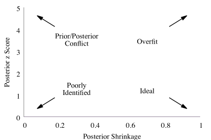
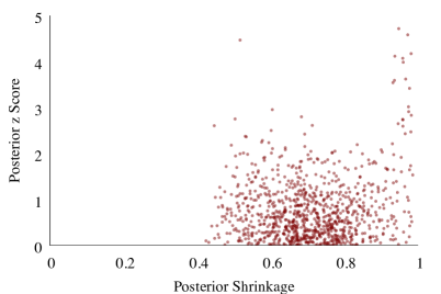
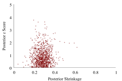
Figure 6: (a) The distribution of posterior $z$-scores and posterior shrinkages with respect to the Bayesian joint distribution identifies well-known pathologies of Bayesian inference. The sensitivity of the posterior to the observations within the scope of a given model can be summarized by sampling from the Bayesian joint distribution, constructing posteriors, and then plotting the corresponding posterior $z$-scores and shrinkages. (b) This model demonstrates good behavior for most observations, with a small tail of outcomes that overfit to a few observations. (c) This model is weakly identified, with the information introduced by the data doing little to improve upon the information encoded in the prior distribution.

3.5 Limitations of Model-Based Calibration

The ultimate limitation of model-based calibration is its dependence on the model configuration space. Any model-based sensitivities or guarantees claimed by model-based calibrations rely on the model configuration space being rich enough to capture the true data generating process, or at least contain model configurations that approximate it sufficiently well.

Unfortunately it is difficult to quantify how these guarantees might change as the as the model configurations become worse approximations to the true data generating process. Consequently it is up to the user to verify the sufficiency of the assumed model configuration space with, for example, predictive validations such as residual analysis for frequentist point estimators or posterior predictive checks for Bayesian analyses.

Another point of fragility of model-based sensitivity and calibrations is that they apply only for the exact models and decisions being considered. If those models or decisions are tweaked then the guarantees no longer need apply. The only way to ensure valid calibrations is to recompute them every time the experiment is modified. An consequence of this fragility is that any sensitivity or calibration is suspect whenever the construction of the model itself depends on the observed data! The only rigorous way to maintain the validity of these results is to consider a larger model that incorporates this implicit dependence of the model configuration space on the observed data.

Because observations are often used to critique and ultimately tune the model, this vulnerability is almost impossible to avoid in practice. Consequently model-based calibration is perhaps best considered as a tool for identifying poorly inferential behaviors in a model rather than making absolute guarantees about its performance.

4 Calibrating Discovery Claims

One of the most common decisions made in the applied sciences is whether or not to claim that a phenomenon in the system being studied exists or doesn’t exist. Whether such discovery claims are good scientific practice is debatable, but given their prevalence it is important to be able to calibrate these decisions regardless.

Many decision making processes have been developed within in both statistics and applied fields, and many of these methods have come under recent scrutiny given their failure to replicate in subsequent experiments. The underlying issue in these failed replications is often poor calibration of the original discovery claim.

In this section I review how discovery claims can be constructed from a statistical model both in the frequentist and Bayesian paradigms and discuss some of the practical issues with their calibration.

4.1 Partitioning the Model Configuration Space

In order to decide on the presence of a phenomenon we need to partition the model configuration space into those model configurations that are influenced by the phenomenon and those that are not. For example we might partition the model configuration space into data generating processes containing only background sources and those containing both signal and background sources. Alternatively we might consider a partition into model configurations where two phenomena manifest distinct behaviors and those where they behave identically. Discovery claims are then informed by which of the two partitions is more consistent with the observed data.

Let the phenomenon of interest be characterized with a subset of parameters, $\vartheta=\varpi(\theta)$, where $\varpi$ projects the total parameter space onto the phenomenological parameters of interest. Additionally assume that the parameters are structured such that $\vartheta=0$ identifies those data generating processes not influenced by the phenomenon being considered. In this case the model configuration space partitions into an absence model

$$\Theta_{1}=\left\{\theta\in\Theta\mid\varpi(\theta)=0\right\},$$

and a complementary presence model,

$$\Theta_{2}=\left\{\theta\in\Theta\mid\varpi(\theta)\neq 0\right\}$$

(Figure 7). This includes the case where $\vartheta$ is constrained to be positive, in which case the presence model reduces to $\theta>0$, or the more general case where $\vartheta$ is unconstrained and the presence model includes all positive and negative, but non-zero, parameters.

Figure 7: When claiming a discovery we first identify the phenomenological parameters, $\vartheta$, which quantify the behavior of a phenomena of interest. The remaining nuisance parameters quantify the behavior of the environment in which the phenomenon interacts and the the measurement process itself. When $\vartheta=0$ identifies a vanishing phenomenon we can partition the full model configuration space into an absence model of those model configurations satisfying $\vartheta=0$ and a presence model of those model configurations satisfying $\vartheta\neq 0$. Discovery is claimed when the presence model is strongly preferred over the absence model by an observation, for various definitions of “preferred”.

For example, consider a model where our observations are generated from overlapping signal and background sources, $\mu_{s}$ and $\mu_{b}$ respectively, with Gaussian measurement variability $\sigma$. This yields the model configuration space

$$\pi(y\mid\mu_{s},\mu_{b},\sigma)=\mathcal{N}(y\mid\mu_{s}+\mu_{b},\sigma).$$

If we are interested in understanding the signal then we would consider the projection

$$\mu_{s}=\vartheta=\varpi(\mu_{s},\mu_{b},\sigma),$$

with the absence model defined as $\mu_{s}=0$, regardless of the value of the nuisance parameters $\mu_{b}$ and $\sigma$, and the presence model as the complement with $\mu_{s}\neq 0$.

Because we don’t know which of the two partitions contains the true data generating process we have to calibrate our decisions with respect to both. In particular we have to consider the probability of claiming a discovery when the true data generating process is in the presence model and when it is in the absence model. We can fully characterize the four possible outcomes with two probabilities: the false discovery rate, $\mathrm{FDR}$ and the true discovery rate, $\mathrm{TDR}$ (Table 1). In classical statistics the false discovery rate is also known as the Type I error while one minus the true discovery rate is also known as the Type II error.

Truth	Decision
	Claim $\theta^{*}\in\Theta_{1}$	Claim $\theta^{*}\in\Theta_{2}$
$\theta^{*}\in\Theta_{1}$ (No Phenomenon)	$\mathrm{FDR}$	$1-\mathrm{FDR}$
$\theta^{*}\in\Theta_{2}$ (Phenomenon)	$1-\mathrm{TDR}$	$\mathrm{TDR}$

Table 1: When preparing to claim a discovery we have to consider the range of inferential outcomes both for when the true data generating process, $\theta^{*}$, is an element of the absence model, $\theta^{*}\in\Theta_{1}$, and when it is an element of the presence model, $\theta^{*}\in\Theta_{2}$. Given the false discovery rate, $\mathrm{FDR}$, and true discovery rate, $\mathrm{TDR}$, we can compute any expected loss with respect to the claiming a discovery or not.

Given these probabilities we can compute the expected loss once we have assigned losses to the possible decision outcomes. For example, let $L_{1}$ be the loss associated with claiming a discovery when the true data generating process is in the absence model and $L_{2}$ the possibly negative loss associated with claiming a discovery when the true data generating process is in the presence model. The expected loss for claiming a discovery is then given by

$$L_{\text{claim discovery}}=(1-\mathrm{FDR})\,L_{1}+\mathrm{TDR}\,L_{2}.$$

In practice we need not limit ourselves to dichotomous decisions. We could also consider a decision process that claims the phenomenon exists, claims the phenomenon doesn’t exist, or makes no claim at all. This process would be characterized by six probabilities, four of which are independent (Table 2). Importantly the expected loss of a discovery claim can be miscalculated if we ignore the possibility that an analysis may not be reported for some observations and the two additional degrees of freedom needed to quantify the expected loss in this more general circumstance.

Truth	Decision
	Claim $\theta^{*}\in\Theta_{1}$	Claim $\theta^{*}\in\Theta_{2}$	Claim Nothing
$\theta^{*}\in\Theta_{1}$ (No Phenomenon)	$p_{1}$	$p_{2}$	$p_{3}$
$\theta^{*}\in\Theta_{2}$ (Phenomenon)	$p^{\prime}_{1}$	$p^{\prime}_{2}$	$p^{\prime}_{3}$

Table 2: A decision process where we can avoid making any claim about the phenomenon of interest by not publishing our analysis is characterized by six probabilities, four of which are independent because of the normalization constraints, $\sum_{n=1}^{3}p_{n}=1$ and $\sum_{n=1}^{3}p^{\prime}_{n}=1$.

4.2 Frequentist Null Hypothesis Significance Testing

The conventional approach to claiming discoveries in a frequentist framework is the null hypothesis significance testing framework. Here the null hypothesis that the true data generating process falls into the absence model is treated as something of a strawman set up to be rejected by observation. In order to reject the null hypothesis we consider how extreme an observation is with respect to the model configurations in the absence model. The more extreme our rejection threshold the smaller the false discovery rate should be.

Naively, if the null hypothesis is rejected then we are left with only the alternative hypothesis that the true data generating process falls into the presence model. That said, we can’t simply reject the null hypothesis in isolation — a poor fit to the null hypothesis does not imply that the alternative hypothesis is any more consistent with the observation! At the very least we have to consider also how likely we are to reject the null hypothesis when the alternative hypothesis is true.

Exactly how the null hypothesis significance testing framework is implemented depends on the structure of the null and alternative hypotheses. The procedure is straightforward for simple hypotheses but quickly becomes difficult to implement in practice as the hypotheses become more complex.

4.2.1 Point Hypotheses

The simplest case of null hypothesis significance testing is when both the null hypothesis and alternative hypothesis are point hypotheses consisting of a single model configuration each. In this case we’ll denote the lone data generating processes in the absence model $\pi_{N}(y)$ and the lone data generating process in the precence model $\pi_{A}(y)$.

For a point null hypothesis we can quantify the extremity of an observation, $\tilde{y}$, with a tail probability or $p$-value,

$$p(\tilde{y})=\int_{\tilde{y}}^{\infty}\mathrm{d}y\,\pi_{N}(y).$$

The integral might be computed analytically or with numerical methods such as quadrature for low-dimensional measurement spaces and Monte Carlo for high-dimensional measurement spaces.

If we reject the null hypothesis when

$$p(\tilde{y})<1-\alpha$$

for some significance, $\alpha$, then by construction the false discovery rate of our claim will be

$$\mathrm{FDR} =\int_{Y}\mathrm{d}y\,\pi_{N}(y)\,\mathbb{I}\left[\,p(y)<1-\alpha\right]$$

$$=\int_{0}^{1}\mathrm{d}\tilde{p}\;\mathbb{I}\left[\,\tilde{p}<1-\alpha\right]$$

$$=1-\alpha.$$

By tuning the significance of the null hypothesis test we can immediately achieve whatever false discovery rate is desired in a given application.

The true discovery rate, also known as the power of the null hypothesis test, is the average null $p$-value with respect to the alternative data generating process,

$$\mathrm{TDR}=\beta=1-\int_{Y}\mathrm{d}y\,\pi_{A}(y)\,p(y).$$

Provided that the power is sufficiently high, observations for which the null hypothesis is rejected will be more consistent with the alternative hypothesis in expectation. There is no guarantee, however, that the alternative will actually be more consistent for every observation.

Unlike the false discovery rate, the true discovery rate is a consequence of the assumed model and cannot be tuned once a significance has been set. Consequently unsatisfactorily low true discovery rates can be remedied only by modifying the experimental circumstances, for example by increasing the number of observations included in each measurement.

4.2.2 Point Null Hypotheses and Complex Alternative Hypotheses

Null hypothesis significance testing becomes more complicated when the model configuration space no longer consists of just two data generating processes and both hypotheses cannot be point hypotheses. Consider next the situation where the null hypothesis is still given by a single data generating process, $\theta=0$, and the alternative hypothesis contains the remaining model configurations $\theta\neq 0$. This might arise, for example, when our model contains only one phenomenological parameter and $\theta=0$ uniquely defines the circumstance where the phenomenon is absent.

As before we can define the $p$-value,

$$p(\tilde{y})=\int_{\tilde{y}}^{\infty}\mathrm{d}y\,\pi(y\mid\theta=0),$$

and then reject the null hypothesis when

$$p(\tilde{y})<1-\alpha$$

to ensure a given false discovery rate.

Unfortunately there is no longer a unique way of defining a power that gives the true discovery rate because the true discovery rate will, in general, be different for each of the model configuration in the alternative hypothesis,

$$\beta_{\theta}=1-\int_{Y}\mathrm{d}y\,\pi(y\mid\theta)\,p(y),\,\theta\neq 0.$$

If $\Theta$ is one-dimensional then we can visualize the sensitivity of the $p$-values as a function of $\theta$ (Figure 8). When $\Theta$ is two-dimensional we can no longer visualize the full variation of the sensitivity distribution, but we can visualize the variation of a summary statistic such as the power (Figure 9). Visualizations allow us to identify regions in the alternative model configuration space of high power, but they do not define a unique power or true discovery rate for the test.

Figure 8: When the model configuration space is one-dimensional we can visualize the sensitivity of the null $p$-values for each of the model configurations in the alternative hypothesis, $\theta\neq 0$. This allows us to quickly communicate the distribution of (a) the null $p$-values, $p(y)$ or the equivalent (b) standard scores $z(y)=\Phi^{-1}(1-p(y))$. Here the distributions are summarized with their medians in dark red and with the quartiles in light red. In particular we can identify which $\theta$ in the alternative hypothesis achieve a given true discovery rate, here $0.999$, by seeing where the central value of the distributions surpass a dashed line.

Figure 9: When the model configuration space is two-dimensional we can visualize how the power, $\beta_{\theta}$, varies with the model configurations in the alternative hypothesis, here $(\theta_{1},\theta_{2})\neq(0,1)$. As in the one-dimensional case we can vary the decoration to identify those model configurations achieving a given true discovery rate, here $0.999$, shown in red.

One immediate strategy is to define an overall power is to consider the minimum power over all of the model configurations in the alternative hypothesis,

$$\beta\equiv\min_{\theta\neq 0}\beta_{\theta}.$$

Provided that we could accurately compute the minimum, this definition would ensure that the overall power lower bounds the true discovery rate for all model configurations in the alternative hypothesis. Unfortunately, when the null hypothesis is nested within the alternative hypothesis the power can become arbitrarily small for the alternative model configurations in the neighborhood around the lone null model configuration. Consequently in practice we will generally be able to claim calibrated discoveries only for a subset of the data generating processes in the alternative hypothesis.

In order to visualize how the power varies with the phenomenological parameters, $\vartheta$, we might also consider defining conditional powers. If the parameters partition into $(\vartheta,\sigma)$, with $\vartheta\in\varpi(\Theta)$ and $\sigma\in\varpi(\Theta)^{C}$, then we could define the conditional power as

$$\beta_{\vartheta}=1-\max_{\sigma\in\varpi(\Theta)^{C}}\int_{Y}\mathrm{d}y\,\pi(y\mid\vartheta,\sigma)\,p(y).$$

Because the optimization of the nuisance parameters, $\sigma$, may be infeasible, profile likelihood methods are often utilized to approximate the conditional powers for visualization. As with any application of asymptotics, the validity of this approximations must be carefully verified for the visualization to be useful.

Finally we might acknowledge the conceptual advantage of having dual point hypotheses and consider not one null hypothesis test but rather an infinite number of tests, where each tests is defined with respect to the point null hypothesis $\theta=0$, and one of the alternative model configurations, $\theta^{\prime}\neq 0$. When we reject the null hypothesis we reject it for any of the alternatives. The preponderance of alternative hypotheses, however, significantly increases the false discovery rate unless we apply a multiple comparison correction to the significance threshold. This increase in the false discovery rate by separating the alternative hypothesis into many point hypothesis is also known as the “look elsewhere effect” in particle physics.

4.2.3 Complex Hypotheses

Unsurprisingly, implementing null hypothesis significance testing becomes all the more difficult when neither the null hypothesis nor the alternative hypothesis are point hypotheses. Given the influence of systematic and environmental factors present in any experiment we rarely if ever enjoy point hypotheses when using realistic models.

When there are multiple model configurations in the null hypothesis we have to consider them all. For example we might define the $p$-value to be the smallest tail probability across all of the null model configurations,

$$p(\tilde{y})=\min_{\theta\in\Theta_{1}}\int_{\tilde{y}}^{\infty}\mathrm{d}y\,\pi(y\mid\theta).$$

If we then reject the null when this minimal $p$-value is less than $1-\alpha$ then the false discovery rate will be at least $\alpha$ for every data generating process in the null hypothesis.

Power and true discover rate calculations proceed as above, with all of the potential complications.

In this general case the computation of the optima needed to bound the false and true discovery rates becomes a particularly significant computational burden that must be addressed with a careful combination of principled assumptions and approximations.

4.2.4 The Likelihood Ratio Test

One of the difficulties with the null hypothesis significance testing framework presented so far is the need to compute tail probabilities over the measurement space. When the measurement space is more than a few dimensions these tail probabilities are difficult to accurately approximate even with substantial computational resources available. A better strategy is to construct a lower-dimensional summary of the measurement space that captures the differences between the null and alternative hypotheses while admitting tests that are easier to implement.

Perhaps the most ubiquitous summary for testing is the likelihood ratio

$$\lambda(\tilde{y})=\frac{\max_{\theta\in\Theta_{1}}\pi(\tilde{y}\mid\theta)}{\max_{\theta\in\Theta}\,\,\pi(\tilde{y}\mid\theta)},$$

which admits the likelihood ratio test where we reject the null hypothesis if $\lambda(\tilde{y})<\lambda_{0}$ for some $0<\lambda_{0}<1$.

The false and true discovery rates of the likelihood ratio test intimately depend on the threshold, $\lambda_{0}$, and the particular structure of the model configuration space. Consequently without further assumptions the likelihood ratio test has to be explicitly calibrated for every application.

The assumption of asymptotics, however, admits an analytic calibration of the likelihood ratio test. Wilk’s Theorem demonstrates that, under the typical asymptotic conditions, the distribution of the logarithm of the likelihood ratio with respect to the model configurations in the null hypothesis asymptotically approaches a $\chi^{2}$ distribution,

$$-2\log\lambda\sim\chi^{2}_{K},$$

with degrees of freedom,

$$K=\mathrm{dim}(\Theta)-\mathrm{dim}(\Theta_{1}).$$

Consequently the false discovery rate for a given threshold, $-2\log\lambda_{0}$, can be calculated by looking up the corresponding $\chi^{2}_{K}$ tail probability.

Indeed theoretical analysis shows that the likelihood ratio test is the optimal test in this asymptotic regime. Many popular tests that have been developed in applied fields, such as the Feldman-Cousins test (Feldman and Cousins, 1998), are actually instances of the likelihood ratio test for specific classes of models.

4.3 Bayesian Model Comparison

Bayesian model comparison is an immediate consequence of extending a probabilistic treatment to the absence and presence partitions of the model configuration space. Given that it’s not conceptually more difficult, however, let’s consider the more general case where we are interested in selecting between one of $N$ models, $\left\{\mathcal{M}_{1},\ldots,\mathcal{M}_{n}\right\}$.

Each model configuration space can have different dimensions, but integrating the parameters out of the corresponding Bayesian joint distribution gives a marginal likelihood over the common measurement space,

$$\pi(y\mid\mathcal{M}_{n}) =\int_{\Theta}\mathrm{d}\theta\,\pi(y,\theta\mid\mathcal{M}_{n})$$

$$=\int_{\Theta}\mathrm{d}\theta\,\pi(y\mid\theta,\mathcal{M}_{n})\,\pi(\theta\mid\mathcal{M}_{n})$$

$$=\mathbb{E}_{\pi(\theta\mid\mathcal{M}_{n})}[\pi(y\mid\theta,\mathcal{M}_{n})].$$

The marginal likelihood is also often known as the Bayes factor or evidence in some fields.

Given the marginal likelihoods we can construct a joint distribution over the measurement and model spaces,

$$\pi(y,\mathcal{M}_{n})=\pi(y\mid\mathcal{M}_{n})\,\pi(\mathcal{M}_{n}),$$

from which Bayes’ Theorem gives the model posteriors,

$$\pi(\mathcal{M}_{n}\mid\tilde{y})=\frac{\pi(\tilde{y},\mathcal{M}_{n})}{\pi(\tilde{y})}=\frac{\pi(\tilde{y}\mid\mathcal{M}_{n})\,\pi(\mathcal{M}_{n})}{\sum_{n^{\prime}=1}^{N}\pi(\tilde{y}\mid\mathcal{M}_{n}^{\prime})\,\pi(\mathcal{M}_{n}^{\prime})}.$$

In particular, given only two models, $\mathcal{M}_{1}$ and $\mathcal{M}_{2}$, we are immediately guided to select the first when it exhibits a higher model posterior density,

$$\pi(\mathcal{M}_{1}\mid\tilde{y}) >\pi(\mathcal{M}_{2}\mid\tilde{y})$$

$$\frac{\pi(\tilde{y}\mid\mathcal{M}_{1})\,\pi(\mathcal{M}_{1})}{\sum_{n^{\prime}=1}^{N}\pi(\tilde{y}\mid\mathcal{M}_{n}^{\prime})\,\pi(\mathcal{M}_{n}^{\prime})} >\frac{\pi(\tilde{y}\mid\mathcal{M}_{2})\,\pi(\mathcal{M}_{2})}{\sum_{n^{\prime}=1}^{N}\pi(\tilde{y}\mid\mathcal{M}_{n}^{\prime})\,\pi(\mathcal{M}_{n}^{\prime})}$$

$$\pi(\tilde{y}\mid\mathcal{M}_{1})\,\pi(\mathcal{M}_{1}) >\pi(\tilde{y}\mid\mathcal{M}_{2})\,\pi(\mathcal{M}_{2})$$

$$\frac{\pi(\tilde{y}\mid\mathcal{M}_{1})}{\pi(\tilde{y}\mid\mathcal{M}_{2})} >\frac{\pi(\mathcal{M}_{2})}{\pi(\mathcal{M}_{1})}.$$

In words, we select $\mathcal{M}_{1}$ when the odds ratio, $\pi(\tilde{y}\mid\mathcal{M}_{1})\,/\,\pi(\tilde{y}\mid\mathcal{M}_{2})$, surpasses a threshold defined by the the relative prior probabilities of the two models, $\pi(\mathcal{M}_{2})/\pi(\mathcal{M}_{1})$. Interestingly this procedure resembles the likelihood ratio test where we use marginal likelihoods instead of maximum likelihoods and the testing threshold is constructed from our prior distributions.

Calibration of this Bayesian model selection then proceeds as with the calibration of any Bayesian inference or decision making processs.

1. We first sample a true model from the model prior,

   $$\mathcal{M}_{\tilde{n}}\sim\pi(\mathcal{M}_{n}).$$

2. Then we sample a true model configuration from the subsequent prior distribution,

   $$\tilde{\theta}\sim\pi(\theta\mid\mathcal{M}_{\tilde{n}}).$$

3. Next we sample an observation from that model configuration,

   $$\tilde{y}\sim\pi(y\mid\tilde{\theta},\mathcal{M}_{\tilde{n}}),$$

4. Finally we calculate the marginal likelihoods to inform model selection,

   $$\pi(\tilde{y}\mid\mathcal{M}_{n}),$$

   and estimate the corresponding discovery rates for each model,

   $$R_{\mathcal{M}_{n}\mid\mathcal{M}_{n^{\prime}}}\approx\frac{\sharp[\text{ Select }{\mathcal{M}_{n}}\text{ given observation from }\mathcal{M}_{n^{\prime}}]}{\sharp[\text{ Observations from }\mathcal{M}_{n^{\prime}}]}.$$

In particular, if we define $\mathcal{M}_{A}$ as the absence model and $\mathcal{M}_{P}$ as the presence model then the false discovery rate is estimated as

$$\mathrm{FDR}\approx\frac{\sharp[\text{ Select }{\mathcal{M}_{P}}\text{ given observation from }\mathcal{M}_{A}]}{\sharp[\text{ Observations from }\mathcal{M}_{A}]}.$$

with the true discovery rate estimated as

$$\mathrm{TDR}\approx\frac{\sharp[\text{ Select }{\mathcal{M}_{P}}\text{ given observation from }\mathcal{M}_{P}]}{\sharp[\text{ Observations from }\mathcal{M}_{P}]}.$$

In cases like this where there are only a few models being considered it may also be easier to condition on each model and compute the corresponding discovery rates one at a time instead of sampling a model at each iteration.

Marginal likelihoods and Bayesian model selection arise immediately once we consider probabilities over the set of models. Unfortunately the theoretical elegance of this approach does not always translate into practical utility.

First and foremost the marginal likelihood is extremely challenging to estimate, even in relatively simple problems. The structure of the integral frustrates typical computational tools like Markov chain Monte Carlo and necessitates more complex, and less well established, tools like nested sampling and simulated tempering. Unfortunately these methods are poorly understood relative to the more established tools and consequently their implementations are still limited by our modest understanding. In particular, quantification of the accuracy of these methods is typically limited to only heuristics.

Beyond the computational issues, however, is a more subtle conceptual issue. The marginal likelihood evaluates a model by comparing a given observation to all of the model configurations in the model configuration space, each weighted by only the prior distribution. Consequently even the smallest details of the prior distribution can significantly affect the marginal likelihood.

This is in stark contrast to the effect of the prior distribution on the posterior distribution. Here the likelihood reduces the influence of model configurations inconsistent with an observation, obscuring much of the structure of the prior distribution. Even seemingly irrelevant details of the prior distribution will still strongly affect the marginal likelihoods, and the practice of constructing prior distributions to ensure only well-behaved posteriors is grossly insufficient for ensuring meaningful marginal likelihoods (Gelman, Simpson and Betancourt, 2017).

In practice the sensitivity of the marginal likelihoods, and hence Bayesian model selection, to the intricate details of the prior distribution manifests in strong dependencies on the observation and a fragility in the corresponding model selection. Small changes in the observation can cause significant changes in the marginal likelihoods, with the decision making process rapidly vacillating amongst the possible models. Fortunately this behavior will manifest in sensitivity analyses and poor false discovery rates and true discovery rates and so it can be quantified provided that the test is calibrated!

4.4 Posterior Probability of The Region of Practical Equivalence

One of the implicit difficulties in informing discovery claims as presented so far is that the absence model is singular with respect to the full model configuration space – the absence model configuration space and the presence model configuration spaces are of different dimensionality. Because of this the posterior probability for all of the model configurations in the absence will always be zero for a prior that is continuous across the full model configuration space. The only way to admit non-zero posterior probabilities over both models is to assign infinitely more prior probability to those model configurations in the absence model relative to those in the presence model.

Bayesian model comparison avoids this issue by comparing only marginal likelihoods and avoiding the individual model posteriors altogether. We can inform a discovery claim using only the posterior over the full model configuration space, however, if we absorb some of the presence model into the absence model. In particular, those model configurations in the presence model close to those in the absence model will generate nearly identical observations and hence indistinguishable inferences; an infinitesimally weak phenomenon will be impossible to differentiate from no phenomenon without an impractical amount of data.

This suggests that we redefine our absence model as

$$\Theta_{1}=\left\{\theta\in\Theta\mid\left|\vartheta(\theta)\right|\leq\vartheta_{0}\right\},$$

with the presence model becoming

$$\Theta_{2}=\left\{\theta\in\Theta\mid\left|\vartheta(\theta)\right|>\vartheta_{0}\right\},$$

for some threshold $\vartheta_{0}$. The neighborhood around the absence model configurations, $\left|\vartheta(\theta)\right|\leq\vartheta_{0}$, is known as the region of practical equivalence (Kruschke, 2014). Notice that separating model configurations close to $\vartheta=0$ from the presence model is not entirely dissimilar in what we had to do when considering the power of a complex alternative model in null hypothesis significance testing.

With this modification of the absence model we can then claim a discovery when the posterior probability in the region of practical equivalence is below a given threshold,

$$\int_{-\vartheta_{0}}^{\vartheta_{0}}\mathrm{d}\theta\,\pi(\vartheta\mid\tilde{y})<1-\alpha,$$

where $\pi(\vartheta\mid\tilde{y})$ is the marginal posterior over the phenomenological parameters.

I have defined the formal decision making process here to superficially resemble that used in null hypothesis significance testing, but we could just as easily use the complementary situation where the posterior probability outside the region of practical equivalence is above the given threshold,

$$\int_{-\infty}^{-\vartheta_{0}}\mathrm{d}\theta\,\pi(\vartheta\mid\tilde{y})+\int_{\vartheta_{0}}^{\infty}\mathrm{d}\theta\,\pi(\vartheta\mid\tilde{y})>1-\alpha.$$

Calibration of this method, in particular the estimation of the false discovery rate and true discovery rate, immediately follows from the Bayesian calibration paradigm.

1. We first sample a true model configuration from the prior distribution over the model configuration space,

   $$\tilde{\theta}\sim\pi(\theta).$$

2. Next we sample an observation from that model configuration,

   $$\tilde{y}\sim\pi(y\mid\tilde{\theta}),$$

3. Finally we reconstruct the posterior probability of the absence model,

   $$P=\int_{-\vartheta_{0}}^{\vartheta_{0}}\mathrm{d}\vartheta\,\pi(\vartheta\mid\tilde{y}).$$

   The false discovery rate follows as

   $$\mathrm{FDR}\approx\frac{\sharp[P\leq 1-\alpha\text{ and }|\varpi(\tilde{\theta})|<\vartheta_{0}]}{\sharp[|\varpi(\tilde{\theta})|<\vartheta_{0}]},$$

   with the true discovery rate,

   $$\mathrm{TDR}\approx\frac{\sharp[P\leq 1-\alpha\text{ and }|\varpi(\tilde{\theta})|>\vartheta_{0}}{\sharp[|\varpi(\tilde{\theta})|>\vartheta_{0}]}.$$

By sampling from various conditional priors we can also quantify how the false and true discovery rates, or even the distribution of $P$ itself, varies with respect to various parameters. This allows us to visualize the sensitivity of the experiment similar to Figure 8, only for arbitrarily complicated models (Figure 10).

Figure 10: By sampling from a conditional joint distribution, $\pi(\sigma\mid\vartheta)$, we can visualize the sensitivity of the distribution of absence model posterior probabilities with respect to a phenomenological parameter, $\vartheta$. The average of this distribution, shown here in dark red, gives the conditional false discovery rate. Given a desired false discovery rate, here $10^{-3}$, we can then identify for which phenomenological parameters we expect a discovery on average, shown here in grey.

4.5 Predictive Scores

Lastly we can select a model and claim discovery or no discovery by comparing the predictive performance of the possible hypotheses. Here we use our inferences to construct a predictive distribution for new data and then select the model whose predictive distribution is closest to the true data generating process.

Predictive distributions arise naturally in many forms of inference. For example, the model configuration identified by a frequentist point estimator defines the predictive distribution

$$\pi_{P}=\pi(y\mid\hat{\theta}(\tilde{y})).$$

Bayesian inference immediately yields two predictive distributions: the prior predictive distribution,

$$\pi_{P}=\pi(y)=\int_{\Theta}\mathrm{d}\theta\,\pi(y\mid\theta)\,\pi(\theta),$$

and the posterior predictive distribuiton,

$$\pi_{P}=\pi(y\mid\tilde{y})=\int_{\Theta}\mathrm{d}\theta\,\pi(y\mid\theta)\,\pi(\theta\mid\tilde{y}).$$

Regardless of how a predictive distribution is constructed, it’s similarity to the true data generating process, $\pi^{*}$, is defined by the Kullback-Leibler divergence,

$$\mathrm{KL}(\pi_{P}\mid\mid\pi^{*}) =\int_{Y}\mathrm{d}y\,\pi^{*}(y)\log\frac{\pi^{*}(y)}{\pi_{P}(y)}$$

$$=\int_{Y}\mathrm{d}y\,\pi^{*}(y)\log\pi^{*}(y)-\int_{Y}\mathrm{d}y\,\pi^{*}(y)\log\pi_{P}(y).$$

Because the first term is the same for all models, the relative predictive performance between models is quantified by the predictive score,

$$S=-\int_{Y}\mathrm{d}y\,\pi^{*}(y)\log\pi_{P}(y).$$

This expectation with respect to the true data generating process cannot be calculated without already knowing the true data generating process, but predictive scores can be approximated using observations which, by construction, are drawn from that distribution. Different approximation methods combined with various predictive distributions yield a host of predictive model comparison techniques, ranging from cross validation to the Akaike Information Criterion, to the Bayesian Information Criterion, to Bayesian cross validation, the Widely Applicable Information Criterion, and the Deviance Information Criterion (Betancourt, 2015).

Error in these approximations, however, can be quite large and difficult to quantify in practice, leading to poorly calibrated selection between the absence model and the presence model. Consequently it is critically important to estimate their expected false discovery rate and true discovery rate using the assumed model. In the frequentist settings these rates can be quantified as the minimal performance across the model configurations in the absence and presence models, where as in the Bayesian setting these rates can be quantified by their expected performance over the Bayesian joint distribution.

5 Applications to Limit Setting

Limit setting is a complement to claiming discovery when the experiment is not expected to be sufficiently sensitive to the relevant phenomenon. Instead of claiming a discovery we consider how strongly we can constrain the magnitude of that phenomenon and calibrate the corresponding constraint with respect to the absence model. Because limit setting is derived from standard inference methods, its implementation is significantly more straightforward than the implementation of discovery claims.

5.1 Frequentist Limit Setting with Anchored Confidence Intervals

In the frequentist setting we can constrain the magnitude of a phenomenon by constructing confidence intervals than span from a vanishing phenomenon to some upper limit. More formally, if the magnitude of the phenomenon is positive, so that the absence model is defined by $\vartheta=0$ and the absence model is defined by $\vartheta>0$, then we construct an anchored confidence interval of the form $\big{[}0,\hat{\vartheta}(y)\big{)}$ that has a given coverage, $\alpha$, with respect to the full model.

Given an observation, $\tilde{y}$, we then claim that $\vartheta<\hat{\vartheta}(\tilde{y})$ with confidence $\alpha$. The sensitivity of this claim is defined with respect to the possible distribution of $\hat{\vartheta}(y)$ with respect to the data generating process in the absence model. For one and two-dimensional absence models the sensitivity can be visualized using the same techniques in Section 4.2.2.

5.2 Bayesian Limit Setting with Posterior Quantiles

The frequentist approach to limit setting has an immediate Bayesian analogue where we use posterior quantiles to bound the magnitude of the phenomenon.

For a given credibility, $\alpha$, we define the upper limit, $\vartheta_{\alpha}$ as

$$\vartheta_{\alpha}(\tilde{y})=\big{\{}\vartheta\mid\int_{0}^{\vartheta}\mathrm{d}\vartheta\,\pi(\vartheta\mid\tilde{y})=1-\alpha\big{\}}.$$

By defining the limit in terms of the marginal posterior for the phenomenological parameters, $\vartheta$, we automatically incorporate the uncertainty in any nuisance parameters into the bound.

The corresponding sensitivity follows by considering the distribution $\vartheta_{\alpha}$ with respect to the Bayesian joint distribution for the absence model.

1. We first sample a true model configuration from the absence model by sampling the nuisance parameters from the conditional prior distribution,

   $$\tilde{\sigma} \sim\pi(\sigma\mid\vartheta=0)$$

   $$\tilde{\theta} =\left(0,\tilde{\sigma}\right).$$

2. Next we sample an observation from that model configuration,

   $$\tilde{y}\sim\pi(y\mid\tilde{\theta}),$$

3. Finally we compute the inferred upper bound,

   $$\vartheta_{\alpha}(\tilde{y})=\big{\{}\vartheta\mid\int_{0}^{\vartheta}\mathrm{d}\vartheta\,\pi(\vartheta\mid\tilde{y})=1-\alpha\big{\}}.$$

6 Conclusions and Future Directions

Both the frequentist and Bayesian perspectives admit procedures for analyzing sensitivities and calibrating decision making processes. Implementing these calibrations in practice, however, is far from trivial.

Frequentist calibration requires bounding the expectation of a given loss function over all of the data generating processes in a given model, or partitions thereof. The derivation of analytic bounds from assumptions about the structure of the model configuration space and the loss function, especially those derived from asymptotic analyses, is greatly facilitated with the presumption of simple model configuration spaces. Numerical methods for computing the bounds are also aided by simple models. The probabilistic computations required of Bayesian calibration are often more straightforward to approximate but sufficiently complex models will eventually frustrate even the most advanced Bayesian computational methods. In practice these computational challenges result in a dangerous tension between models that are simple enough to admit accurate calibrations and models that are complex enough for their resulting calibrations to be relevant to the experiment being analyzed.

The continued improvement in computational resources and algorithms has gradually reduced, and promises to continue to reduce, this tension. Monte Carlo and Markov chain Monte Carlo methods, for example, have revolutionized our ability to compute expected losses and Bayesian posterior expectations over high-dimensional measurement and model configuration spaces. Unfortunately the applicability of this method critically depends on the desired calibration. In particular, the square root convergence of Monte Carlo estimators is often too slow to ensure accurate calibration of rare observations. This frustrates the calculation, for example, of the $\mathcal{O}(1-10^{-7})$ significance thresholds presumed in contemporary particle physics. Computational limitations restrain not only the complexity of our models but also the complexity of the loss function we consider.

Statistics is a constant battle between computational feasibility and compatibility with analysis goals. Ultimately it is up to the practitioner to exploit their domain expertise to identify compromises that facilitate high-performance decision making.

Finally there is the issue of experimental design where we tune the design of an experiment to achieve a given performance. As difficult as it is to compute this performance, “inverting” the calibration to identify the optimal experiment is even harder. For complex models that don’t admit analytic results, contemporary best practice often reduces to exploring the experiment design space heuristically, guided by computed calibrations and domain expertise.

An interesting future direction is the use of automatic differentiation methods to automatically estimate not only the expected losses but also their gradients with respect to the experimental design. Although an imposing implementation challenge, these gradients have the potential to drastically improve the exploration and optimization of experimental designs.

7 Acknowledgements

I thank Lindley Winslow, Charles Margossian, Joe Formaggio, and Dan Simpsons for helpful comments and discussions.

References

- Bernardo and Smith (2009) {bbook}[author] \bauthor\bsnmBernardo, \bfnmJose-M.\binitsJ.-M. and \bauthor\bsnmSmith, \bfnmAdrian F. M.\binitsA. F. M. (\byear2009). \btitleBayesian Theory. \bseriesWiley Series in Probability and Mathematical Statistics: Probability and Mathematical Statistics. \bpublisherJohn Wiley & Sons, Ltd., Chichester. \endbibitem
- Betancourt (2015) {barticle}[author] \bauthor\bsnmBetancourt, \bfnmMichael\binitsM. (\byear2015). \btitleA Unified Treatment of Predictive Model Comparison. \endbibitem
- Betancourt (2017) {barticle}[author] \bauthor\bsnmBetancourt, \bfnmMichael\binitsM. (\byear2017). \btitleA Conceptual Introduction to Hamiltonian Monte Carlo. \endbibitem
- Brooks et al. (2011) {bbook}[author] \beditor\bsnmBrooks, \bfnmSteve\binitsS., \beditor\bsnmGelman, \bfnmAndrew\binitsA., \beditor\bsnmJones, \bfnmGalin L.\binitsG. L. and \beditor\bsnmMeng, \bfnmXiao-Li\binitsX.-L., eds. (\byear2011). \btitleHandbook of Markov Chain Monte Carlo. \bpublisherCRC Press, \baddressNew York. \endbibitem
- Casella and Berger (2002) {bbook}[author] \bauthor\bsnmCasella, \bfnmGeorge\binitsG. and \bauthor\bsnmBerger, \bfnmRoger L\binitsR. L. (\byear2002). \btitleStatistical inference, \beditionSecond ed. \bpublisherDuxbury Thomson Learning. \endbibitem
- Cook, Gelman and Rubin (2006) {barticle}[author] \bauthor\bsnmCook, \bfnmSamantha R\binitsS. R., \bauthor\bsnmGelman, \bfnmAndrew\binitsA. and \bauthor\bsnmRubin, \bfnmDonald B\binitsD. B. (\byear2006). \btitleValidation of software for Bayesian models using posterior quantiles. \bjournalJournal of Computational and Graphical Statistics \bvolume15 \bpages675–692. \endbibitem
- Feldman and Cousins (1998) {barticle}[author] \bauthor\bsnmFeldman, \bfnmGary J\binitsG. J. and \bauthor\bsnmCousins, \bfnmRobert D\binitsR. D. (\byear1998). \btitleUnified approach to the classical statistical analysis of small signals. \bjournalPhysical Review D \bvolume57 \bpages3873. \endbibitem
- Gelman, Simpson and Betancourt (2017) {barticle}[author] \bauthor\bsnmGelman, \bfnmAndrew\binitsA., \bauthor\bsnmSimpson, \bfnmDaniel\binitsD. and \bauthor\bsnmBetancourt, \bfnmMichael\binitsM. (\byear2017). \btitleThe prior can often only be understood in the context of the likelihood. \bjournalEntropy \bvolume19 \bpages555. \endbibitem
- Gelman et al. (2014) {bbook}[author] \bauthor\bsnmGelman, \bfnmAndrew\binitsA., \bauthor\bsnmCarlin, \bfnmJohn B.\binitsJ. B., \bauthor\bsnmStern, \bfnmHal S.\binitsH. S., \bauthor\bsnmDunson, \bfnmDavid B.\binitsD. B., \bauthor\bsnmVehtari, \bfnmAki\binitsA. and \bauthor\bsnmRubin, \bfnmDonald B.\binitsD. B. (\byear2014). \btitleBayesian Data Analysis, \beditionthird ed. \bseriesTexts in Statistical Science Series. \bpublisherCRC Press, Boca Raton, FL. \endbibitem
- Keener (2011) {bbook}[author] \bauthor\bsnmKeener, \bfnmRobert W\binitsR. W. (\byear2011). \btitleTheoretical statistics: Topics for a core course. \bpublisherSpringer. \endbibitem
- Kruschke (2014) {bbook}[author] \bauthor\bsnmKruschke, \bfnmJohn\binitsJ. (\byear2014). \btitleDoing Bayesian data analysis: A tutorial with R, JAGS, and Stan. \bpublisherAcademic Press. \endbibitem
- Lehmann and Casella (2006) {bbook}[author] \bauthor\bsnmLehmann, \bfnmErich L\binitsE. L. and \bauthor\bsnmCasella, \bfnmGeorge\binitsG. (\byear2006). \btitleTheory of point estimation. \bpublisherSpringer Science & Business Media. \endbibitem
- Robert and Casella (1999) {bbook}[author] \bauthor\bsnmRobert, \bfnmChristian P\binitsC. P. and \bauthor\bsnmCasella, \bfnmGeorge\binitsG. (\byear1999). \btitleMonte Carlo Statistical Methods. \bpublisherSpringer New York. \endbibitem
- Yao et al. (2018) {barticle}[author] \bauthor\bsnmYao, \bfnmYuling\binitsY., \bauthor\bsnmVehtari, \bfnmAki\binitsA., \bauthor\bsnmSimpson, \bfnmDaniel\binitsD. and \bauthor\bsnmGelman, \bfnmAndrew\binitsA. (\byear2018). \btitleYes, but Did It Work?: Evaluating Variational Inference. \endbibitem