Large large-trader activity weakens the long memory of limit order markets

Abstract

Using more than 6.7 billions of trades, we explore how the tick-by-tick dynamics of limit order books depends on the aggregate actions of large investment funds on a much larger (quarterly) timescale. In particular, we find that the well-established long memory of market order signs is markedly weaker when large investment funds trade either in a directional way and even weaker when their aggregate participation ratio is large. Conversely, we investigate to what respect a weaker memory of market order signs predicts that an asset is being actively traded by large funds. Theoretical arguments suggest two simple mechanisms that contribute to the observed effect: a larger number of active meta-orders and a modification of the distribution of size of meta-orders. Empirical evidence suggests that the number of active meta-orders is the most important contributor to the loss of market order sign memory.

1 Introduction

Financial market dynamics is complex in part because of the very large variety of timescales at play. Both traders and volatility feedback loops are known to have widely distributed timescales (Lynch and Zumbach, 2003; Lillo, 2007; Zhou et al., 2011; Tumminello et al., 2012; Challet et al., 2016). Accordingly, investigating how timescales interact reveals some of the fundamental dynamical ingredients of price dynamics. For example, the asymmetric relationship between historical and realized volatility shows that price dynamics is not symmetric with respect to time reversal (Lynch and Zumbach, 2003; Zumbach, 2009), which imposes a strong constraint on realistic stochastic volatility models (Blanc et al., 2017).

The long memory of the signs of market orders is a well-established stylized fact of limit order books (Bouchaud et al., 2004; Lillo and Farmer, 2004) that passes the most stringent statistical tests. Lillo et al. (2005) propose a mathematical framework that links the long memory of these signs to the way very large orders are split into a series of smaller market orders (thereby creating a meta-order) and is able to reproduce the empirical auto-correlation function if the distribution of the meta-order size has a Pareto-like tail. In other words, the shape of the sign auto-correlation function reflects that of the distribution of the size of meta-orders.

Here, we use two large databases of almost maximally different timescales, namely quarterly filings by large investment funds and a comprehensive tick-by-tick database, which allow us to investigate the influence of large funds on the memory properties of the limit order book. We first show that the memory length of market order signs (buy/sell) of a given asset is markedly weaker when a large fraction of its capitalization is exchanged by large funds over a quarter. Reciprocally, we test if assets with the weakest market order sign memory are likely to being much traded by large funds. Finally, we use the theoretical framework of Lillo et al. (2005) to put forward a coherent picture of our findings.

2 The data

Our dataset consists of two databases: quarterly snapshots of large investment ownership, from the corresponding FactSet database in the 2007-2013 period (32 reports), which contains data 10845 funds with more than USD 100 millions under management. We filter out funds with less than USD 100’000 invested into securities. The remaining funds are invested in 12531 securities. We focus on the 2480 assets continuously recorded in FactSet database after their first quarter of appearance and with at least one full year of record. Using automated methods, we link assets found in both FactSet and the Thomson Reuters Tick History databases. The latter provides an event-by-event history of limit order books. For each asset traded on the NASDAQ and each day, we extracted all the trade prices together with the best bid and ask prices just before the trades. Finally, we keep assets traded for at least 200 days and with more than 200 trades per day on average. This leaves 846 stocks and more than 6.7 billion trades.

3 Methods

In order to link trade-by-trade data with quarterly fund filings, we define suitable quantities in each dataset and investigate how they are related. For each asset $\alpha$, we compute the mid-price just before the $n$-th trade, denoted by $m_{\alpha,n}$ as the average between the best bid and ask prices. Then we define the sign of the $n$-th market order of asset $\alpha$ as

$$\epsilon_{\alpha,n}=\text{sign}(p_{\alpha,n}-m_{\alpha,n}).$$

We drop trades that occur exactly at the previous mid-price. As suggested by the above notation, we define the time as the number of market orders since the beginning of the time-series.

3.1 Microstructure: memory length of market order sign auto-correlation

We define several simple ways to characterize the memory of market order signs. Unless specified otherwise, all market microstructure quantities are measured over a full trading week. The first one consists in measuring the probability of the occurrence of $\kappa$ consecutive trades of a given sign in a random contiguous subset of $\{s_{n}\}$. Mathematically, for a generic $\kappa$, this amounts to measuring the conditional event frequency

$$\pi_{\alpha}^{(s\kappa)}=P(s_{n}=s_{n+1}=\cdots=s_{n+\kappa}=s)$$ (1)

for both $s\in\{-1,1\}$.

Another way to characterize the memory of order signs is the market order sign autocorrelation at lag $\tau$ (in unit of market orders), denoted by $C_{\alpha}(\tau)$. Process $\epsilon_{n}^{\alpha}$ has a long memory if the integral of its autocorrelation function $C_{\alpha}$ diverges. Many references find that $C_{\alpha}(\tau)\propto a\tau^{-b}$ where $b<1$, in which case the integral of $C_{\alpha}(\tau)$ is infinite (see e.g. Lillo et al. (2005); Toth et al. (2015)) (we omit the $\alpha$ index for $a$ and $b$ in order to avoid too heavy notations). This is indeed a good approximation for very long time series. For finite time series of length $N$, one can define the effective memory length as the lag $\tau_{\alpha}^{*}$ after which $C_{\alpha}$ reaches for the first time the noise level of autocorrelation functions $2/\sqrt{N}$, i.e., $\tau_{\alpha}^{*}$ is such that $C_{\alpha}(\tau)>2/\sqrt{N}\,\,\,\forall\tau\leq\tau_{\alpha}^{*}$ . We will also consider the scaled maximum lag $\tau_{\alpha}^{*}/N$.

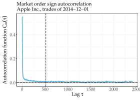
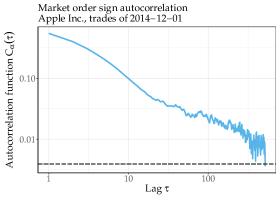
Figure 1: Example of market order sign autocorrelation functions with linear axis scales (left plot) and log-log axis scales (right plot). The black dashed horizontal line is the noise level $2/\sqrt{N}$ where $N$ is the length of the market order sign time series. The black dashed vertical line corresponds to the maximum lag $\tau^{*}$. Apple Inc., trades of 2014-12-01.

3.2 Macro-dynamics: directional fund activity ratio

First, we introduce a quantity that measures, for a given asset $\alpha$, the rescaled global directional change of ownership averaged over all the funds between the quarter ends $q-1$ and $q$. We will call it the directional fund activity ratio and define it as

$$r_{\alpha}(q)=\frac{\sum_{i}[W_{i\alpha}(q)-W_{i\alpha}(q-1)]}{V_{\alpha}(q)},$$ (2)

where $W_{i\alpha}(q)$ is the position in dollars of fund $i$ on security $\alpha$ at the end of quarter $q$, and $V_{\alpha}$ the total volume-dollar of security $\alpha$ exchanged between $q-1$ and $q$. If $r_{\alpha}(t)>0$ (resp. $r_{\alpha}(t)<0$) then the security $\alpha$ is more bought (resp. sold) than sold (resp. bought) by the large funds in our database. We will focus on $R_{\alpha}(q)=|r_{\alpha}(q)|$.

3.3 Macro-dynamics: absolute fund activity ratio

Another important measure of aggregate fund behaviour consists in quantifying how much the investment has changed in absolute terms. We thus define $S_{\alpha}(q)$ as the rescaled absolute difference of invested amounts between quarter ends $q-1$ and $q$, i.e.,

$$S_{\alpha}(q)=\frac{\sum_{i}|W_{i\alpha}(q)-W_{i\alpha}(q-1)|}{V_{\alpha}(q)}.$$ (3)

This quantity cannot account for round trips of funds over a quarter, which are fortunately very unlikely for the largest values of $S$ , i.e., the values relevant to the present work. In addition, when the relative influence on $S$ of large fund round-trips is negligible, $S$ is a good approximation of large fund participation ratio.

4 Results

4.1 From large fund behaviour to microstructure dynamics

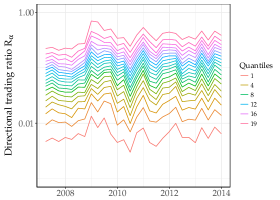
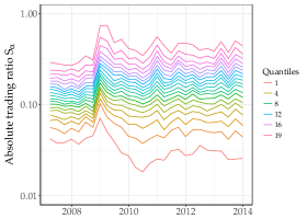
Figure 2: Time evolution of the quantiles of the directional fund activity ratio $R_{\alpha}\left(q\right)$ (left plot) and of the absolute fund activity ratio $S_{\alpha}\left(q\right)$ (right plot).

The premise of this paper is that relating tick-by-tick order book properties to the fund ownership database is easiest when the aggregate behaviour of large investment funds is the most extreme, which corresponds to large values of either $R_{\alpha}$ or $S_{\alpha}$. Thus for each quarter $q$, we divide the assets into 20 groups of $R_{\alpha}(q)$ by computing the quantiles $k_{R}\in\{1,\cdots,19\}$; we do the same for $S_{\alpha}(q)$, yielding $k_{S}\in\{1,\cdots,19\}$. We first compare the microstructural dynamics of the top and bottom groups of both quantities. By convention, the bottom groups $g_{X}=1$ correspond to small values of $X\in\{R,S\}$, i.e., to securities that are bought and sold equally ($R$) or not much traded by large funds ($S$). Figure 2 shows the time evolution of the quantiles of the ratios $R_{\alpha}(q)$ and $S_{\alpha}(q)$. The large-$R$ quantile are clearly correlated with the large-$S$ quantiles. This should be expected, as a large $R_{\alpha}$ implies a large $S_{\alpha}$.

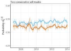
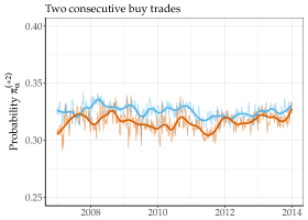
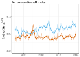
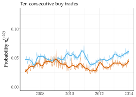
Figure 3: Time evolution of $\pi_{\alpha}^{(\kappa)}$, the probability of observing $\kappa$ consecutive negative trade signs (left plots) and $\kappa$ consecutive positive trade signs (right plots) for the top and bottom quantiles of $R_{\alpha}(q)$ (orange and blue lines, respectively).

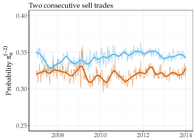
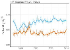
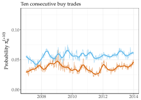
Figure 4: Time evolution of $\pi_{\alpha}^{(\kappa)}$, the probability of observing $\kappa$ consecutive negative trade signs (left plots) and $\kappa$ consecutive positive trade signs (right plots) for the top and bottom quantiles of $S_{\alpha}(q)$ (orange and blue lines, respectively).

Focusing on the assets belonging to the top and bottom groups determined by the quantiles of $R$ and $S$, one now assess the influence of trading by large funds on the market order sign memory length measures. Starting with the two extreme groups determined by the quantiles of $R$, Fig. 3 reports that the frequency of $\kappa$ consecutive trades of the same sign $\pi_{\alpha}^{(s\kappa)}$ for $\kappa=2$, once averaged over all assets belonging to a given group, is consistently different between the two groups of assets as time goes on; one also sees that the difference is larger for $\kappa=10$ than for $\kappa=2$; in fact, it is an increasing function of $\kappa$, at least for $2\leq\kappa\leq 10$. The difference is larger when the assets are grouped according to the quantiles of $S$, as illustrated in Fig.4. In short, being actively traded by large funds decreases the probability of occurrence of consecutive market orders of the same kind, which thus is a sign of weakening of market order sign memory.

The other measures of memory length lead to the same conclusion. For example, fitting the trade sign autocorrelation $C_{\alpha}(\tau)$ with $a\tau^{-b}$ for $\alpha$ in the top and bottom groups of assets consistently yields smaller values of the prefactor $a$ for the quantiles of either $R$ or $S$ (top plots of Fig. 5), except in 2008-2009 with respect to the quantiles of $R$: during this period, $a$ was roughly the same in both groups. The similar behaviour of $\pi_{\alpha}^{(s\kappa)}$ and $a$ is to be expected: $C_{\alpha}(\tau)$ being a function of $\{\pi_{\alpha}^{(s\kappa)}\}_{\kappa}$, the prefactor $a$ is mostly related to small-$\kappa$ probabilities $\pi_{\alpha}^{(s\kappa)}$. The case of the exponent $b$ is more nuanced and revealingly so (bottom-left plot of Fig. 5): large directional trading by large funds has no clear influence on $b$, except in times of crisis, as e.g. in 2008-2009 when assets with large $R$ a smaller $b$ than the assets in the small-$R$ group. The 2011 crisis also lead to a significant and similar influence of $R$ on $b$; while the typical value of $a$ of assets with a large $R$ plunged, it did not reach that of assets with small $R$, contrarily to what happened during the 2008-2009 period. The absolute activity ratio $S$ has always been discriminant for $a$. Regarding $b$, assets with a large $S$ also had a smaller $b$ (but a large $a$) in 2008-2009, while in the 2012-2014 period, the reverse is true. Thus these fitting parameters provide a more dynamic picture on the influence of the activity of large funds.

The overall picture is nevertheless the same: for a given number of trades, on average, the difference of $a$ and $b$ between the top and bottom quantiles of $R$ and $S$ contribute to shorten the length of the memory as inferred by $C_{\alpha}(\tau)$ because the noise level is reached at smaller lags for assets in the top quantiles. This is indeed confirmed by Fig. 6 which shows the time evolution of the $\tau_{\alpha}^{*}$ averaged over the top and bottom quantiles of $R$ and $S$. One notes that $\tau_{\alpha}^{*}$ of the top and bottom groups are clearly separated, while this ceases to be the case for and $\tau_{\alpha}^{*}/N$ since 2012. The effect of $R$ or $S$ is opposite on $\tau_{\alpha}^{*}$ and $\tau_{\alpha}^{*}/N$, which is due to the fact that the number of transactions $N$ of assets with large $R$ or $S$ is typically smaller.

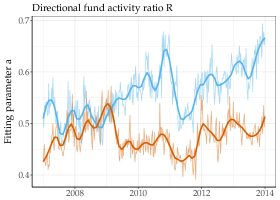
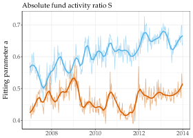
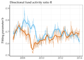
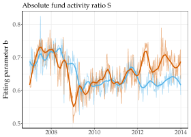
Figure 5: Time evolution of the fitting parameters characterizing the long memory of the market order sign autocorrelation $C_{\alpha}(\tau)=a\tau^{b}$. Top plots: evolution of $a$ averaged over all the members of the bottom and top quantile of $R_{\alpha}(q)$ (left plot) and $S_{\alpha}\left(q\right)$ (right plot). Bottom plots: evolution of $b$ averaged over all the members of the bottom and top quantiles (orange and blue lines, respectively) of $R_{\alpha}(q)$ (left plot) and $S_{\alpha}(q)$ (right plot).

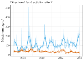
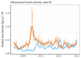
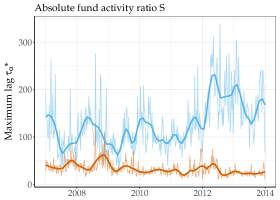
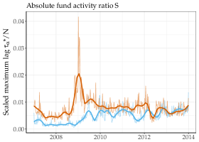
Figure 6: Time evolution of $\tau_{\alpha}^{*}$, the scaled maximum lag before the autocorrelation function of the trade signs reaches the noise level, averaged over the top and bottom quantiles (orange and blue lines, respectively) of $R_{\alpha}(q)$ (upper plots) and $S_{\alpha}(q)$ (bottom plots).

4.2 Large fund directional and absolute trading detection

A more relevant question in practice is whether one can detect trading by large investment funds from quantities measured from tick-by-tick data. In the context of this paper, the question may be rephrased as how to guess in which quantile of $R$ or $S$ a given asset may be from the knowledge of $a$, $b$, $\tau^{*}$ or $\tau^{*}/N$. Since the later quantities are measured of a week, we compute with their averages over a given quarter.

Here, we focus on the following simple classification problem: for each quarter, we split the 20 groups into two categories according to quantile $k_{\text{cut}}$: assets belonging to the quantiles $k\leq k_{\text{cut}}$ form the first category and the remaining ones the other one. Choosing a memory length measure as the variable according to which one classifies the assets during a given quarter, it is then straightforward to compute the parametric Receiver Operating Characteristic (ROC) curve and its associated area under curve (AUC) for a given quarter. Figure 7 reports the AUC associated with $\pi^{(s10)}$, $a$, $b$, $\tau^{*}$ and $\tau^{*}/N$ for the quantiles of both $R$ and $S$, averaged over the 32 quarters. One sees that $\pi^{(s10)}$ and $a$ are roughly equivalent and are the best variables to discriminate the large values of $R$ and $S$. Even more, their detection power with respect to the quantiles of $S$ does not depend much on $k_{\text{cut}}$.

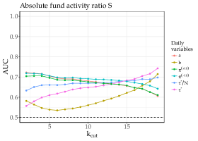
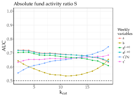
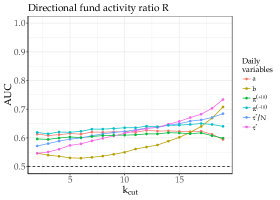
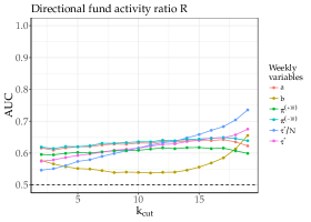
Figure 7: Average quarterly Area Under Curve (AUC) corresponding to the classification of funds belonging to quantile $k\geq k_{\text{cut}}$ for each market order sign memory length measures. Left plot: averages of daily microstructural quantities; right plot: averages of weekly microstructural quantities. AUC averaged over the whole history.

5 A theoretical insight

Lillo et al. (2005) establish the link between the size of meta-orders and the order sign auto-correlation. In particular, they find that if the distribution of the size $L$ of meta-orders, denoted by $P(L)$, has a power-law tail $P(L)\propto L^{-(\beta+1)}$, then, assuming that the sign order of each meta-order is equiprobably $-1$ or $+1$ and that there are exactly $M$ active meta-orders at any time for a given asset, the auto-correlation function is given by $C(\tau)\simeq a\tau^{-b}=\frac{M^{\beta-2}}{\beta}\tau^{-(\beta-1)}$ for large $\tau$. This simple relationship gives two insights relevant to our results.

First, the pre-factor $a$ is a decreasing function of $M$ when $\beta<2$, which is generally the case as $\beta\simeq 1.5$ on average for example in the London Stock Exchange (Lillo et al., 2005). Identifying $\beta-1$ with $b$ here shows that in our case $b<1$, hence that $\beta<2$. This implies that the pre-factor $a$ is a proxy for the number of meta-orders present in the market, ceteribus paribus, which should then be strongly related to $S$. This is why the pre-factor $a$ (and thus $\pi^{(10)}$) are among the best predictors of the quantile range of $S$ (Fig.  5).

Second, $b$ being a proxy for an effective $\beta$, it allows to gain some insight on the tail of $P(L)$. Since the measured $b$ decreases, the probability of very large meta-orders increases, which is coherent with directional trading from large funds after large price changes. Another explanation for the change of $b$ resides in the the way meta-orders are split: there must be feedback loops between the exponent $\beta$ and the available liquidity which in turns most probably depends on the current order flow, determined in part by meta-orders.

6 Concluding remarks

This work has brought to light the fact that the influence of the trading of large funds on the memory of market order signs is far from negligible: large funds do not suppress long memory, but may weaken it. When one knows ex postfacto how large funds have traded, there is a clear difference between limit order book dynamics in which large fund took a substantial part and those barely touched by them (relatively speaking). Reversely, even when averaging the market order sign memory length measures over a quarter allows to some extend to predict if large funds have been much involved in the trading of a given asset.

The main limitation of the present work is the use of quarterly data to characterise fund behaviour. Using labelled trades would open the way to relate the properties of order book day by day and and to improve our understanding of the link between the composition of meta-orders and the memory length of market order signs.

References

- Blanc et al. [2017] Pierre Blanc, Jonathan Donier, and J-P Bouchaud. Quadratic hawkes processes for financial prices. Quantitative Finance, 17(2):171–188, 2017.
- Bouchaud et al. [2004] Jean-Philippe Bouchaud, Yuval Gefen, Marc Potters, and Matthieu Wyart. Fluctuations and response in financial markets: the subtle nature of ’random’ price changes. Quantitative finance, 4(2):176–190, 2004.
- Challet et al. [2016] Damien Challet, Rémy Chicheportiche, Mehdi Lallouache, and Serge Kassibrakis. Trader lead-lag networks and order flow prediction. 2016.
- Lillo [2007] Fabrizio Lillo. Limit order placement as an utility maximization problem and the origin of power law distribution of limit order prices. The European Physical Journal B, 55(4):453–459, 2007.
- Lillo and Farmer [2004] Fabrizio Lillo and J Doyne Farmer. The long memory of the efficient market. Studies in nonlinear dynamics & econometrics, 8(3), 2004.
- Lillo et al. [2005] Fabrizio Lillo, Szabolcs Mike, and J Doyne Farmer. Theory for long memory in supply and demand. Physical review e, 71(6):066122, 2005.
- Lynch and Zumbach [2003] Paul Lynch and Gilles Zumbach. Market heterogeneities and the causal structure of the volatility. Quantitative Finance, 3:320–331, 2003.
- Toth et al. [2015] Bence Toth, Imon Palit, Fabrizio Lillo, and J Doyne Farmer. Why is equity order flow so persistent? Journal of Economic Dynamics and Control, 51:218–239, 2015.
- Tumminello et al. [2012] M. Tumminello, F. Lillo, J. Piilo, and R.N. Mantegna. Identification of clusters of investors from their real trading activity in a financial market. New Journal of Physics, 14:013041, 2012.
- Zhou et al. [2011] Wei-Xing Zhou, Guo-Hua Mu, Wei Chen, and Didier Sornette. Investment strategies used as spectroscopy of financial markets reveal new stylized facts. PloS one, 6(9):e24391, 2011.
- Zumbach [2009] Gilles Zumbach. Time reversal invariance in finance. Quantitative Finance, 9(5):505–515, 2009.