Abstract

Low-complexity non-smooth convex regularizers are routinely used to impose some structure (such as sparsity or low-rank) on the coefficients for linear predictors in supervised learning. Model consistency consists then in selecting the correct structure (for instance support or rank) by regularized empirical risk minimization. It is known that model consistency holds under appropriate non-degeneracy conditions. However such conditions typically fail for highly correlated designs and it is observed that regularization methods tend to select larger models. In this work, we provide the theoretical underpinning of this behavior using the notion of mirror-stratifiable regularizers. This class of regularizers encompasses the most well-known in the literature, including the $\ell_{1}$ or trace norms. It brings into play a pair of primal-dual models, which in turn allows one to locate the structure of the solution using a specific dual certificate. We also show how this analysis is applicable to optimal solutions of the learning problem, and also to the iterates computed by a certain class of stochastic proximal-gradient algorithms.

1 Introduction

Regularized empirical risk minimization.

We consider a general set-up for supervised learning where, given an input/output space $\mathcal{X}\times\mathcal{Y}$ endowed with a probability measure $\rho$, one wants to learn an estimator $f:\mathcal{X}\rightarrow\mathcal{Y}$ satisfying $f(x)\approx y$ for $\rho$-a.e. pair of data $(x,y)\in\mathcal{X}\times\mathcal{Y}$. We restrict ourselves to the case where $\mathcal{X}\times\mathcal{Y}=\mathbb{R}^{p}\times\mathbb{R}$, with $p$ being the dimension of the feature space, and we search for an estimator that is linear in $\mathcal{X}$, meaning that $f$ can be written $f_{w_{0}}(x)=\langle x,\,w_{0}\rangle$ for some coefficient vector $w_{0}\in\mathbb{R}^{p}$. A standard modeling assumption is that, among the minimizers of a quadratic expected risk, $w_{0}$ possesses some form of simplicity or low-complexity (e.g. sparsity or low-rank). In other words, $w_{0}$ is assumed to be the unique solution of

$$\min_{w\in\mathbb{R}^{p}}\!\left\{\!R(w)\!\!\;:\;\!\!w\in\underset{w^{\prime}\in\mathbb{R}^{p}}{\operatorname{Argmin}}\;\mathbb{E}_{\rho}\!\left[(\langle w^{\prime},\,\mathrm{\bf x}\rangle-\mathrm{\bf y})^{2}\right]\!\right\} \text{P}_{0}$$ ()

where $R:\mathbb{R}^{p}\rightarrow\mathbb{R}\cup\{+\infty\}$ is a proper lower semi-continuous (l.s.c.) convex regularizer, and $\mathbb{E}_{\rho}\left[{\cdot}\right]$ is the expectation of the random variable $(\mathrm{\bf x},\mathrm{\bf y})$ w.r.t. the probability measure $\rho$.

In practice ($\text{P}_{0}$) cannot be solved directly because one does not have access to $\rho$; only a sequence of $n$ independent and identically distributed (i.i.d.) pairs $(x_{i},y_{i})_{i=1}^{n}$ sampled from $\rho$ is available. The conventional approach is then to consider a solution $\widehat{w}_{\lambda,n}$ of a penalized empirical risk minimization (ERM) of the form

$$\min_{w\in\mathbb{R}^{p}}\lambda R(w)+\!\frac{1}{2n}\sum_{i=1}^{n}\left(\langle x_{i},\,w\rangle-y_{i}\right)^{2}\!. \text{P}_{\lambda,n}$$ ()

The regularization parameter $\lambda>0$ is tuned as a (decreasing) function of $n$, balancing appropriately between fitting the data and inducing some desirable property promoted by the regularizer $R$.

Tracking the structure of the solution.

A theoretical question in statistical learning is to understand how close a solution $\widehat{w}_{\lambda,n}$ of ($\text{P}_{\lambda,n}$) comes to $w_{0}$. If $\widehat{w}_{\lambda_{n},n}\rightarrow w_{0}$ (convergence being usually considered in probability) as $n\rightarrow+\infty$ with $\lambda_{n}\rightarrow 0$, then the estimator is said to be consistent. One is also generally interested in stating estimation rates, and a linear estimation rate corresponds to $|\!|\widehat{w}_{\lambda_{n},n}-w_{0}|\!|\sim n^{-\frac{1}{2}}$ (to be understood in probability). Note that we are here discussing guarantees on the estimation risk and not on the prediction risk (i.e. on $w$ and not on $f_{w}(x)=\langle w,\,x\rangle$), which is more challenging. In this paper, we investigate model consistency, that is, whether $w_{\lambda_{n},n}$ and $w_{0}$ share the same structure for appropriately chosen $\lambda_{n}$ and $n$ large enough. Existing results on the subject heavily rely on a non-degeneracy condition at $w_{0}$, which is often referred as an “irrepresentable condition” (see more details and references in Remark 1). In this case, one can show that for $n$ large enough and $\lambda_{n}\sim n^{-1/2}$, model consistency holds; see for $\ell_{1}$ (Zhao and Yu,, 2006), $\ell_{1}$-$\ell_{2}$ (Bach, 2008a, ), nuclear norm (Bach, 2008b, ) and more generally for the class of partly-smooth functions (Vaiter et al.,, 2014). The first goal of this paper is to go one step further by formally analyzing the general and challenging case where the non-degeneracy assumption cannot be guaranteed.

Tracking the structure of proximal algorithms.

Similar consistency questions arise for the approximations of solutions computed by stochastic proximal algorithms used to solve ($\text{P}_{\lambda,n}$). Many non-smooth low-complexity structure-promoting regularizers are such that their proximal operator is easy to compute either explicitly (as for the $\ell_{1}$ norm or the trace norm) or approximately to good precision (as for the total variation in one-dimension). Proximal-gradient algorithms are then the methods of choice for solving the structured optimization problem ($\text{P}_{\lambda,n}$). For large-scale machine learning problems, one would typically prefer stochastic versions of these algorithms, which need only one observation to proceed with the iterate; see e.g. (A. Defazio and Lacoste-Julien,, 2014; Xiao and Zhang,, 2014). The second goal is then to understand if these iterates and $w_{0}$ share the same structure induced by $R$. This complements the existing convergence analysis of these algorithms; pointers to relevant literature are given in Section 3.

Paper organization.

As explained above, this paper has two goals about general model consistency for (i) regularized learning models and (ii) stochastic algorithms for solving them. The low-complexity induced by popular regularizers reveals primal-dual partitions which allow us to localize optimal solutions and track iterates. Section 2 recalls the notion of mirror-stratifiable regularizers which provides this structural complexity partition. Then Section 3 states our model recovery results and discusses their originality with respect to the existing literature. The rationale and the milestones of the proofs are sketched in Section 4; details and technical results are established in the supplementary material. Finally Section 5 provides numerical illustrations of our results, giving theoretical justification of typical observed behaviors of stochastic algorithms.

2 Low-complexity models

Low-complexity and stratification.

In this paper, we study model consistency for a large class of regularizers, and under few structural assumptions. Our results strongly rely on duality arguments, and on a structure induced by $\partial R$ (where $\partial R$ is the subdifferential of $R$). To track the structure of solutions, we introduce an appropriate stratification $\mathcal{M}=\{M_{i}\}_{i\in I}$ of $\operatorname{dom}(\partial R)\subset\mathbb{R}^{p}$ (where $\operatorname{dom}(\partial R):=\left\{w\in\mathbb{R}^{p}\;:\;\partial R(w)\neq\emptyset\right\}$), which is a finite partition such that for any strata $M$ and $M^{\prime}$

$$~{}M\cap\operatorname{cl}(M^{\prime})\neq\emptyset~{}\Rightarrow M\subset\operatorname{cl}(M^{\prime})$$

(where $\operatorname{cl}$ stands for the topological closure of the set). Because this is a partition, any element $w\in\operatorname{dom}(\partial R)$ belongs to a unique stratum, which we denote $M_{w}$. A stratification also induces a partial ordering $\leqslant$ as follows

$$M\!\leqslant\!M^{\prime}\Longleftrightarrow M\!\subset\!\operatorname{cl}(M^{\prime})\Longleftrightarrow M\!\cap\!\operatorname{cl}(M^{\prime})\!\neq\!\emptyset.$$ (1)

With such ordering, it is natural to see some strata as being “smaller” than others, and, by extension, to say that the elements of such small strata have a low-complexity.

Example 1.

Most regularizers $R$ used in machine learning naturally come up with a stratification, in the sense that they promote solutions belonging to small (for the relation $\leqslant$) strata $M$.

• Lasso (Tibshirani,, 1996): the simplest example is the $\ell_{1}$ norm where $R(w)=\sum_{i}|w_{i}|$, where the strata are the sets of vectors $M_{I}=\left\{w\in\mathbb{R}^{p}\;:\;\operatorname{supp}(w)=I\right\}$, where $I\subset\{1,\cdots,p\}$.

• Nuclear (a.k.a. trace) norm (Fazel,, 2002): this is another popular example where $R(w)$ is the $\ell_{1}$ norm of the singular values of $w$, and where the strata are the manifolds of fixed-rank matrices: $M_{r}=\left\{w\in\mathbb{R}^{p_{1}\times p_{2}}\;:\;\operatorname{rank}(w)=r\right\}$, where $r\in\{0,\cdots,\min(p_{1},p_{2})\}$.

• Many other examples fall within this class of regularizers. For instance the $\ell_{1}$-$\ell_{2}$-norm to promote group-sparsity (Yuan and Lin,, 2005), or the fused Lasso (Tibshirani et al.,, 2005). Yet another example is the total variation semi-norm $R(w)=|\!|Dw|\!|_{1}$ where $D$ is a discrete approximation to the “gradient” operator (on a regular grid or on a graph); in this case, the strata are defined by piecewise constant vectors sharing the same jump set (edges in signals or images).

Mirror-Stratifiable Regularizers.

All the classical regularizers mentioned in Example 1 have moreover a strong relation between their primal and dual stratifications. These primal-dual relations are defined through the following correspondence operator $\mathcal{J}_{R}$ between subsets $S\subset\mathbb{R}^{p}$,

$$\mathcal{J}_{R}(S):=\bigcup_{x\in S}\operatorname{ri}(\partial R(x)),$$

where $\operatorname{ri}$ denotes the relative interior of a convex set. Following Fadili et al., (2017), we define mirror-stratifiabilty as follows.

Definition 1.

Let $R$ be a proper lsc and convex function and $R^{*}$ its Legendre-Fenchel conjugate. $R$ is mirror-stratifiable with respect to a (primal) stratification $\mathcal{M}=\{M_{i}\}_{i\in I}$ of $\operatorname{dom}(\partial R)$ and a (dual) stratification $\mathcal{M}^{*}=\{M^{*}_{i}\}_{i\in I}$ of $\operatorname{dom}(\partial R^{*})$ if $\mathcal{J}_{R}:\mathcal{M}\to\mathcal{M}^{*}$ is invertible with inverse $\mathcal{J}_{R^{*}}$ and $\mathcal{J}_{R}$ is decreasing for the relation $\leqslant$ defined by (1).

This structure finds its roots in (Daniilidis et al.,, 2014), which introduces the tools to show that polyhedral functions, as well as spectral lifting of polyhedral functions, are mirror-stratifiable. In particular, all popular regularizers mentioned above ($\ell_{1}$ norm, $\ell_{1}$-$\ell_{2}$ mixed norms, nuclear norm, total variation semi-norm) are mirror-stratifiable; see (Fadili et al.,, 2017).

Example 2.

Let us illustrate this notion in the case $R=\|\cdot\|_{1}$. As mentioned in Example 1, the strata $M_{I}$ of $\operatorname{dom}(\partial R)=\mathbb{R}^{p}$ are sets of sparse vectors, with prescribed support. In the dual, $\operatorname{dom}(\partial R)^{*}$ is the unit $\ell_{\infty}$-ball, which can be naturally stratified by sets of vectors in $[-1,1]^{p}$ with a prescribed active set. More precisely, if we define

$$\operatorname{active}(\eta):=\left\{i\in\{1,\cdots,p\}\;:\;|\eta_{i}|=1\right\},$$

then these strata are of the form $M^{*}_{I}=\left\{\eta\in[-1,1]^{p}\;:\;\operatorname{active}(\eta)=I\right\}$. It is then an easy exercise to verify that the following correspondence operators $\mathcal{J}_{R}$ and $\mathcal{J}_{R^{*}}$ induce a decreasing bijection between the dual strata $M^{*}_{I}$ and the primal strata $M_{I}$, meaning that:

$$(\forall I,J\subset\{1,\cdots,p\})\quad \mathcal{J}_{R}(M_{I})=M^{*}_{I},\ \mathcal{J}_{R^{*}}(M^{*}_{I})=M_{I}$$

and $$I\subset J\Leftrightarrow M_{I}\leqslant M_{J}\Leftrightarrow M_{I}^{*}\geqslant M_{J}^{*}.$$

All the regularizers in Example 1 work in the same way. For instance, for the nuclear norm, the strata $M_{r}$ made of rank-$r$ matrices are in correspondence with strata $M^{*}_{r}$ made of matrices having exactly $r$ singular values equal to $1$, and the others being of smaller amplitude.

3 Main results

We study model consistency by bypassing unrealistic assumptions (e.g., irrepresentable-type condition) and thus obtain flexible theoretical results. Throughout this paper, we only assume the following hypotheses:

$$\begin{cases}\text{$R$ is mirror-stratifiable},\\ \text{$R$ is bounded from below},\\ \text{$w_{0}$ is the unique solution of~{}\eqref{Eq:primal expected problem}}.\\ \end{cases} \text{H}_{\text{M}}$$ ()

Under ($\text{H}_{\text{M}}$), we establish general model consistency results of optimal solutions of the regularized ERM problem ($\text{P}_{\lambda,n}$) (in Section 3.1), and of iterates of stochastic proximal algorithms to solve it (in Section 3.2). We also discuss how these results encompass the existing model consistency results (in Section 3.3).

Our analysis leverages the strong primal-dual structure of mirror-stratifiable regularizers, which is our key tool to localize the active strata at the solution of ($\text{P}_{\lambda,n}$), even in the case where the irrepresentable condition is violated. We show that an enlarged model consistency holds, where the identified structure lies between the ideal one (the structure of $w_{0}$) and a worst-case one controlled by a particular dual element (the so-called dual vector/certificate)

$$\eta_{0}\in\partial R(w_{0}),$$

defined as the optimal solution

$$\eta_{0}=\operatorname{Argmin}\left\{\langle C^{\dagger}\eta,\,\eta\rangle\!\!\;:\;\!\!\eta\in\partial R(w_{0})\cap\operatorname{Im}C\right\} \text{D}_{\text{0}}$$ ()

where $C:=\mathbb{E}_{\rho}\left[\mathrm{\bf x}\mathrm{\bf x}^{\top}\right]\in\mathbb{R}^{p\times p}$ is the expected (non-centered) covariance matrix, and $C^{\dagger}$ denotes its Moore-Penrose pseudo-inverse. The role of $\eta_{0}$ in sensitivity analysis of regularized ERM problems is well-known, but has been always done under a non-degeneracy assumption (see forthcoming discussions in Remark 1 and Section 3.3).

3.1 Model consistency for regularized ERM

Our first contribution, Theorem 1 below, states that for an appropriate regime of $(\lambda_{n},n)$, one can precisely localize with probability $1$ the active stratum at $\widehat{w}_{\lambda_{n},n}$ between a minimal active set associated to $w_{0}$ and a maximal one controlled by the dual vector $\eta_{0}$. In the special case of $\ell_{1}$ minimization, this means that, almost surely, the support of $\widehat{w}_{\lambda_{n},n}$ can be larger than that of $w_{0}$ but cannot be larger than the extended support characterized by $\operatorname{active}(\eta_{0})$. This holds provided that $\lambda_{n}$ decreases to $0$ with $n$, but not too fast to account for errors stemming from the finite sampling.

Theorem 1.

Assume that ($\text{H}_{\text{M}}$) holds, and suppose that $\mathbb{E}_{\rho}\left[\|\mathrm{\bf x}\|^{4}\right]<+\infty$ and $\mathbb{E}_{\rho}\left[|\mathrm{\bf y}|^{4}\right]<+\infty$. Let $(\lambda_{n})_{n\in\mathbb{N}}\subset]0,+\infty[$ be such that

$$\lambda_{n}\to 0\text{\quad with\quad$\lambda_{n}\sqrt{n/(\log\log n)}\to+\infty$}.$$

Then, for $n$ large enough, the following holds with probability $1$:

$$M_{w_{0}}\leqslant M_{\widehat{w}_{\lambda_{n},n}}\leqslant\mathcal{J}_{R^{*}}(M_{\eta_{0}}^{*}).$$ (2)

Example 3.

Using the notations of Example 1 and 2, the enlarged consistency (2) specializes to

$$\operatorname{supp}(w_{0})\subset\operatorname{supp}(\widehat{w}_{\lambda_{n},n})\subset\operatorname{active}(\eta_{0}),$$

$$\operatorname{rank}(w_{0})\leqslant\operatorname{rank}(\widehat{w}_{\lambda_{n},n})\leqslant\#\left\{s\in\sigma(\eta_{0})\;:\;|s|=1\right\},$$

for the $\ell_{1}$ norm and the nuclear norm, respectively. $\sigma(\eta_{0})$ denotes the vector of singular values of $\eta_{0}$.

The theorem guarantees that we have an enlarged model consistency, as soon as enough data is sampled. The first interest of this result is the finite identification, compared to the existing asymptotic results (even if the level of generality does not allow us to provide a bound on $n$); we discuss this in Section 3.3. The second and main advantage of our result is that it does not require any unrealistic non-degeneracy assumption. We explain this point in the next two remarks, by looking at the usual assumption and how it often fails to hold in high dimension.

Remark 1 (Irrepresentable condition and exact model consistency).

If it is furthermore assumed that

$$\eta_{0}\in\operatorname{ri}(\partial R(w_{0})),$$ (IC)

then it follows from Definition 1 that $M_{w_{0}}=\mathcal{J}_{R^{*}}(M_{\eta_{0}}^{*})$. In that setting, the consistency (2) just gives exact model consistency

$$M_{w_{0}}=M_{\widehat{w}_{\lambda_{n},n}}.$$

This relative interiority assumption (IC) corresponds exactly to the “irrepresentable condition” which is classical in the learning literature (Zhao and Yu,, 2006),(Bach, 2008a, ),(Bach, 2008b, ). Without this non-degeneracy hypothesis, we cannot expect to have exact model consistency (this is for instance illustrated in Section 5). The above theorem shows that there is still an approximate optimal model consistency, with two extreme strata fully characterized by the primal-dual pair $(w_{0},\eta_{0})$. Our result is thus able to explain what is going on in the intricate situation where (IC) is violated.

Remark 2 (When the irrepresentable condition fails).

The originality and interest of our model consistency result is that condition (IC) is not required to hold, since it is usually not valid in the context of large-scale learning. Let us give some insights on this condition in the specific case of $\ell_{1}$-regularized problems. For instance, if the $x_{i}$’s are drawn from a standard Gaussian i.i.d. distribution, the compressed sensing literature provides sample thresholds depending on the dimension $p$ and the sparsity level $s=\|w_{0}\|_{0}$. In this scenario, it is known that uniqueness in ($\text{H}_{\text{M}}$) holds for $n>2s\log(p/s)$ (Amelunxen et al.,, 2014), while the irrepresentable condition holds only for $n>2s\log(p)$ (Candes and Recht,, 2013): the gap between these thresholds corresponds to the case where (IC) fails. Observe nevertheless that these results rely on the assumption that the features are incoherent (here Gaussian i.i.d.), which is not likely to be verified in a learning scenario, where they are typically highly correlated. A setting with a coherent operator $C$ is that of deconvolution, where $C$ is a (discerete) convolution operator associated to a smooth kernel, which is widely studied in the signal/image processing literature (in particular for the super-resolution). In this case, one can exactly determine the largest manifold $\mathcal{J}_{R^{*}}(M^{*})$ involved in (2), see (Duval and Peyré,, 2017).

3.2 Model consistency for stochastic proximal-gradient algorithms

Our second main result describes model consistency for the iterates generated by a stochastic algorithm. In our situation, the general (relaxed) stochastic proximal gradient algorithm for solving ($\text{P}_{\lambda,n}$) reads, starting from any initialization $\widehat{w}^{0}$, at iteration $k$:

$$\begin{cases}\widehat{d}^{k}=(\langle\widehat{w}^{k},x_{i(k)}\rangle-y_{i(k)})x_{i(k)}+\widehat{\varepsilon}^{k},\\ \widehat{z}^{k}=\operatorname{prox}_{\gamma_{k}\lambda R}(\widehat{w}^{k}-\gamma_{k}\widehat{d}^{k}),\\ \widehat{w}^{k+1}=(1-\alpha_{k})\widehat{w}^{k}+\alpha_{k}\widehat{z}^{k},\end{cases}$$ (RSPG)

where $(x_{i(k)},y_{i(k)})$ are independent random variables drawn among $(x_{i},y_{i})_{i=1}^{n}$, $\gamma_{k}\in]0,+\infty[$ and $\alpha_{k}\in]0,1]$ are respectively deterministic stepsize and relaxation parameters. As it is, the iteration is written in an abstract way, since we do not specify how to define the random $\mathbb{R}^{p}$-valued variables $\widehat{\varepsilon}^{k}$. But as we explain below, several known stochastic methods can be written under the form of (RSPG) when $\alpha_{k}\equiv 1$.

Example 4.

If one takes $\widehat{\varepsilon}^{k}\equiv 0$, then (RSPG) becomes simply the proximal stochastic gradient method (Prox-SGD). Variance-reduced methods, like the SAGA algorithm (A. Defazio and Lacoste-Julien,, 2014), or the Prox-SVRG algorithm (with option I) (Xiao and Zhang,, 2014), also fall into this scheme. For these algorithms the idea is to take $\widehat{\varepsilon}^{k}$ as a combination of previously computed estimates of the gradient, in order to reduce the variance of $\widehat{d}^{k}$. For instance, SAGA corresponds to the choice:

$$\widehat{\varepsilon}^{k}=\frac{1}{n}\sum\limits_{i=1}^{n}g_{k,i}-g_{k,i(k)}$$

where the stored gradients are updated as

$$g_{i,k}:=\begin{cases}(\langle\widehat{w}^{k},x_{i(k)}\rangle-y_{i(k)})x_{i(k)}&\text{if }i=i(k)\\ g_{k-1,i}&\text{else.}\end{cases}$$

We show in Theorem 2 that for $n$ large enough and $\lambda_{n}$ appropiately chosen, we can identify after a finite number of iterations of (RSPG) an active stratum, which is again localized between two strata controlled by $w_{0}$ and $\eta_{0}$, respectively. For this result to hold, we have to make some reasonable assumptions on algorithm (RSPG). We need first to make hypotheses on the parameters $\alpha_{k}$, $\gamma_{k}$, $\widehat{\varepsilon}^{k}$, to ensure that the iterates of (RSPG) converge to a solution of ($\text{P}_{\lambda,n}$). Such hypotheses have been investigated in (Combettes and Pesquet,, 2016; Rosasco et al.,, 2016; Atchadé et al.,, 2017) to establish useful convergence results. Beyond convergence, we study structure identification of these algorithms. It is known that convergence is not enough for model consistency of iterates. For instance, the classical proximal stochastic gradient method (corresponding to the case $\widehat{\varepsilon}^{k}\equiv 0$) is known to fail at generating sparse iterates for the case $R=\|\cdot\|_{1}$; see below Example 5 for discussions and references. To ensure the identification of low-dimensional strata, we require some control on the variance of the descent direction, by acting either on the parameters $\gamma_{k}$ and $\alpha_{k}$, or by wisely controlling $\widehat{\varepsilon}^{k}$. Before stating formally this set of hypotheses, we introduce $L_{n}:=(1/n)\|\sum_{i=1}^{n}x_{i}x_{i}^{*}\|$ and the $\sigma$-algebra $\mathcal{F}_{k}:=\sigma(\widehat{w}^{1},\dots,\widehat{w}^{k})$ generated by the first $k$ iterates.

$$\begin{cases}\sigma_{k}\in[0,+\infty[,\ \alpha_{k}\in]0,1],\ \gamma_{k}\in]0,2/L_{n}[\\[3.44444pt] \mathbb{E}\left[\widehat{\varepsilon}^{k}|\mathcal{F}_{k}\right]=0,\ \operatorname{Var}\left[\widehat{d}^{k}|\mathcal{F}_{k}\right]\leqslant\sigma_{k}^{2}\\ \ \widehat{d}^{k}-\mathbb{E}\left[\widehat{d}^{k}|\mathcal{F}_{k}\right]\text{ converges a.s. to }0\\[0.86108pt] \sum_{k=1}^{\infty}\alpha_{k}\gamma_{k}^{2}\sigma_{k}^{2}<+\infty\\[4.30554pt] |\!|\widehat{w}^{k+1}-\widehat{w}^{k}|\!|=o(\alpha_{k}\gamma_{k})\ \text{a.s.}\end{cases} \text{H}_{\text{A}}$$ ()

Let us briefly discuss these hypotheses. The second line in ($\text{H}_{\text{A}}$) imposes some control on the variance of $\widehat{d}^{k}$. The fourth line asks for a fine balance between the parameters $\alpha_{k}$, $\gamma_{k}$ and $\sigma_{k}$. For instance, one could take $\alpha_{k}$ and $\gamma_{k}$ to be constant, and work essentially on $\widehat{\varepsilon}^{k}$ to ensure that $\sigma_{k}\in\ell^{2}(\mathbb{N})$ and $\widehat{w}^{k}$ is a.s. asymptotically regular. Instead, one could consider an algorithm where $\sigma_{k}$ does not vanish, but with appropriately decreasing step-sizes: $\gamma_{k}$ and $\alpha_{k}$ should be carefully chosen to guarantee that the fourth row of ($\text{H}_{\text{A}}$) holds.

Theorem 2.

Assume that ($\text{H}_{\text{M}}$) holds, and suppose that $\mathbb{E}\left[\|\mathrm{\bf x}\|^{4}\right]<+\infty$ and $\mathbb{E}\left[|\mathrm{\bf y}|^{4}\right]<+\infty$. Let $(\lambda_{n})_{n\in\mathbb{N}}\subset]0,+\infty[$ be such that

$$\lambda_{n}\to 0\quad\text{with $\lambda_{n}\sqrt{n/(\log\log n)}\to+\infty$}.$$

Then, for $n$ large enough, if $(\widehat{w}^{k})_{k\in\mathbb{N}}$ is generated by (RSPG) under assumption ($\text{H}_{\text{A}}$), then for $k$ large enough:

$$M_{w_{0}}\leqslant M_{\widehat{z}^{k}}\leqslant\mathcal{J}_{R^{*}}(M_{\eta_{0}}^{*})\quad\text{ holds almost surely}.$$

Example 5.

Let us look at two instances of (RSPG).

• The SAGA (resp. Prox-SVRG) algorithm is shown to verify ($\text{H}_{\text{A}}$) in (Poon et al.,, 2018), provided that $\alpha_{k}\equiv 1$ and $\gamma_{k}\equiv\gamma=1/(3L_{n})$ (resp. $\gamma_{k}\equiv\gamma$ taken small enough).

• The proximal stochastic gradient method (Prox-SGD) is a specialization of (RSPG) with $\alpha_{k}\equiv 1$, $(\gamma_{k})_{k\in\mathbb{N}}\in\ell^{2}(\mathbb{N})\setminus\ell^{1}(\mathbb{N})$ and $\widehat{\varepsilon}^{k}\equiv 0$. If the iterates are bounded, the second line of ($\text{H}_{\text{A}}$) automatically holds by the (strong) law of large numbers. Nevertheless, this algorithm does not satisfy the conclusions of Theorem 2: this was observed in (Xiao,, 2010; Lee and Wright,, 2012; Poon et al.,, 2018), and is illustrated in Section 5. A simple explanation is that for this algorithm, $\sigma_{k}$ does not converge to 0, which is why we need to impose that the stepsize $\gamma_{k}$ tends to zero. Even if it can be shown that $|\!|\widehat{w}^{k+1}-\widehat{w}^{k}|\!|/\gamma_{k}$ is bounded, it cannot be ensured that it is $o(1)$, which breaks the last hypothesis in ($\text{H}_{\text{A}}$). Thus Theorem 2 does not apply in agreement with the observed behaviour of the SGD algorithm.

3.3 Relation to previous results.

Model consistency of the regularized ERM has already been investigated for special cases ($\ell_{1}$ (Zhao and Yu,, 2006), $\ell_{1}$-$\ell_{2}$ (Bach, 2008a, ), or nuclear norm (Bach, 2008b, )) and for the class of partly-smooth functions (Vaiter et al.,, 2014). The existing results hold asymptotically in probability, e.g. of the form

$$\lim\limits_{n\to+\infty}\mathbb{P}\left(M_{w_{0}}=M_{\widehat{w}_{\lambda_{n},n}}\right)=1,$$ (3)

while we show that the consistency (2) holds almost surely, as soon as enough data is sampled. Nevertheless, our result lacks a quantitative estimation of how large $n$ should be for the identification to hold. As a comparison, (Vaiter et al.,, 2014) shows that the probability in (3) converges as $1-n^{-1/2}$, but the result heavily relies on the assumption that (IC) holds (which prevents the solution from “jumping” between the strata $M_{w_{0}}$ and $\mathcal{J}_{R^{*}}(M^{*}_{\eta_{0}})$). Such qualitative estimates cannot be derived in our more general results without stronger assumptions and/or structure, which we want to avoid.

Compared to previous works, a chief advantage of our model consistency results is thus to avoid making an assumption which often fails to hold in high dimension. Indeed, as explained in Remark 2 and Section 5, the above-mentioned existing results hold under the irrepresentable condition (IC); and many of these also assume that the expected covariance matrix $C=\mathbb{E}_{\rho}\!\left[\mathrm{\bf x}\mathrm{\bf x}^{\top}\right]$ is invertible. The first work to deal with model consistency for a large class of functions without the irrepresentable condition assumption is (Fadili et al.,, 2017), which introduces of the notion of mirror-stratifiable functions, from which the authors derive identification properties of a deterministic penalized problem. Our Theorem 1 comes with a similar flavor, but extended to a supervised learning scenario and random sampling, which brought technical challenges as detailed in Section 4.

Finite activity identification for stochastic algorithms has been a topic of interest in the past years. (Xiao,, 2010) made the observation that Prox-SGD has not the identification property for the $\ell_{1}$ case. Instead, finite activity identification was proved by Lee and Wright, (2012), for the regularized dual averaging (RDA) method, and by Poon et al., (2018), for the SAGA and Prox-SVRG algorithms. For these two papers, the regularizer $R$ is assumed to be partly-smooth, and a non-degeneracy assumption is made. Again, Theorem 2 does not need such an assumption. We also propose a general set of hypotheses ($\text{H}_{\text{A}}$) encompassing all these algorithms and beyond: this allows an explanation for why Prox-SGD fails (see Example 5), and could be used to analyze other algorithms than SAGA or Prox-SVRG.

4 Sketch of proofs

Our model consistency results follow from a sequence of results controlling the behaviour of optimal solutions and of iterates of algorithms. In this section, we sketch the rationale and the milestones of the proof; the proof of the two intermediate technical results are given in the supplementary material.

The core of the proofs rely on (Fadili et al.,, 2017, Theorem 1) about sensivity analysis of mirror-stratifiable functions. We state this result here in a modified form that is adapted to our analysis.

Proposition 1.

Let $R$ be mirror-stratifiable. Then, there exists $\delta>0$ such that for any pair $\eta\in\partial R(w)$,

$$\max\{|\!|w-w_{0}|\!|,|\!|\eta-\eta_{0}|\!|\}\leqslant\delta\Rightarrow M_{w_{0}}\leqslant M_{w}\leqslant\mathcal{J}_{R^{*}}(M_{\eta_{0}}^{*}).$$

Proof.

Suppose for contradiction that no such $\delta$ exists. Let $(\delta_{k})_{k\in\mathbb{N}}\subset]0,+\infty[$ and $(w^{k},\eta^{k})_{k\in\mathbb{N}}\subset\operatorname{gph}(\partial R)$ be such that $\delta_{k}\downarrow 0$, $\max(|\!|w^{k}-w_{0}|\!|,|\!|\eta^{k}-\eta_{0}|\!|)\leqslant\delta_{k}$, but where $M_{w^{k}}$ does not satisfy the claimed inequalities. Then $(w^{k},\eta^{k})\to(w_{0},\eta_{0})$ as $k\to\infty$, and $(w_{0},\eta_{0})\in\operatorname{gph}(\partial R)$ by definition in ($\text{D}_{\text{0}}$). Upon applying (Fadili et al.,, 2017, Theorem 1), we have that $M_{w_{0}}\leqslant M_{w^{k}}\leqslant\mathcal{J}_{R^{*}}(M_{\eta_{0}}^{*})$ for $k$ sufficiently large. This is a contradiction with the choice of $w^{k}$. ∎

Concerning Theorem 1, we introduce the notations

$$\widehat{C}_{n} :=\frac{1}{n}\sum_{i}x_{i}x_{i}^{\top}\in\mathbb{R}^{p\times p},$$

$$\widehat{u}_{n} :=\frac{1}{n}\sum_{i}y_{i}x_{i}\in\mathbb{R}^{p},\quad u:=\mathbb{E}_{\rho}\left[\mathrm{\bf y}\mathrm{\bf x}\right],$$

which allows us to rewrite problems ($\text{P}_{0}$) and ($\text{P}_{\lambda,n}$) in a compact form:

$$\{w_{0}\} =\underset{w\in\mathbb{R}^{p},Cw=u}{\operatorname{Argmin}}\;R(w),$$

$$\widehat{w}_{\lambda,n} \in\underset{w\in\mathbb{R}^{p}}{\operatorname{Argmin}}\;\lambda R(w)+\frac{1}{2}\langle\widehat{C}_{n}w,w\rangle-\langle\widehat{u}_{n},w\rangle.$$

The optimality conditions for ($\text{P}_{\lambda,n}$) allow to derive:

$$\widehat{\eta}_{\lambda_{n},n}\in\partial R(\widehat{w}_{\lambda_{n},n}),\quad\widehat{\eta}_{\lambda_{n},n}:=\frac{\widehat{u}_{n}-\widehat{C}_{n}\widehat{w}_{\lambda_{n},n}}{\lambda_{n}}.$$ (4)

In view of Proposition 1, establishing Theorem 1 essentially boils down to showing the following proposition. The proof of this proposition requires technical lemmas to control the interlaced effects of convergence and sampling; see the supplementary material for details.

Proposition 2.

Under the assumptions of Theorem 1, $(\widehat{w}_{\lambda_{n},n},\widehat{\eta}_{\lambda_{n},n}){\underset{n\to+\infty}{\longrightarrow}}$ $(w_{0},\eta_{0})$ almost surely.

From Proposition 2, we deduce that there exists $N\in\mathbb{N}$ such that for all $n\geqslant N$:

$$\max\{|\!|\widehat{w}_{\lambda_{n},n}-w_{0}|\!|,|\!|\widehat{\eta}_{\lambda_{n},n}-\eta_{0}|\!|\}\leqslant\delta/2\quad a.s.$$ (5)

Using Proposition 1, we deduce that (2) holds a.s. for all $n\geqslant N$. To prove Theorem 2, we keep $n\geqslant N$ fixed, and consider $(\widehat{w}^{k})_{k\in\mathbb{N}}$ to be generated by the (RSPG) algorithm. Using the definition of $\widehat{w}^{k+1}$, we can write

$$\widehat{z}^{k} =\widehat{w}^{k}+\frac{\widehat{w}^{k+1}-\widehat{w}^{k}}{\alpha_{k}},$$ (6)

$$\widehat{w}^{k}-\gamma_{k}\widehat{d}^{k} \in\widehat{z}^{k}+\gamma_{k}\lambda_{n}\partial R(\widehat{z}^{k}).$$ (7)

Let us introduce

$$h_{n}(w) :=(1/2n)\sum_{i=1}^{n}(\langle w,x_{i}\rangle-y_{i})^{2}$$

$$\widehat{\xi}^{k} :=\widehat{\varepsilon}^{k}-\nabla h_{n}(\widehat{w}^{k})+(\langle w,x_{i(k)}\rangle-y_{i(k)})x_{i(k)},$$

so that (6) and (7) can be rewritten as

$$\widehat{v}^{k}:=\frac{\widehat{w}^{k}-\widehat{w}^{k+1}}{\alpha_{k}\gamma_{k}}-\xi_{k}-\nabla{h_{n}}(\widehat{w}^{k})\in\lambda_{n}\partial R(\widehat{z}^{k}).$$ (8)

The missing block to conclude the proof of Theorem 2 is then the next proposition whose proof is in the supplementary material.

Proposition 3.

Let $n\in\mathbb{N}$, $\lambda_{n}\in]0,+\infty[$, and let $(\widehat{w}^{k})_{k\in\mathbb{N}}$ be generated by the (RSPG) algorithm under assumption ($\text{H}_{\text{A}}$). Then $(\widehat{z}^{k},\widehat{v}^{k})$ converges almost surely to $(\widehat{w}_{\lambda_{n},n},\widehat{\eta}_{\lambda_{n},n})$, as $k\to+\infty$.

We can now complete the proof of Theorem 2 as follows. In light of Proposition 3, we deduce that there exists $K\in\mathbb{N}$ such that for all $k\geqslant K$,

$$\max\{|\!|\widehat{w}_{\lambda_{n},n}-\widehat{z}^{k}|\!|,|\!|\widehat{\eta}_{\lambda_{n},n}-\widehat{v}^{k}|\!|\}\leqslant\delta/2\quad a.s.$$

Without loss of generality, we can assume that the limit of the algorithm is the $\widehat{w}_{\lambda_{n},n}$ appearing in (5). The above inequality, combined with (5), allows us to use Proposition 1, and this proves Theorem 2.

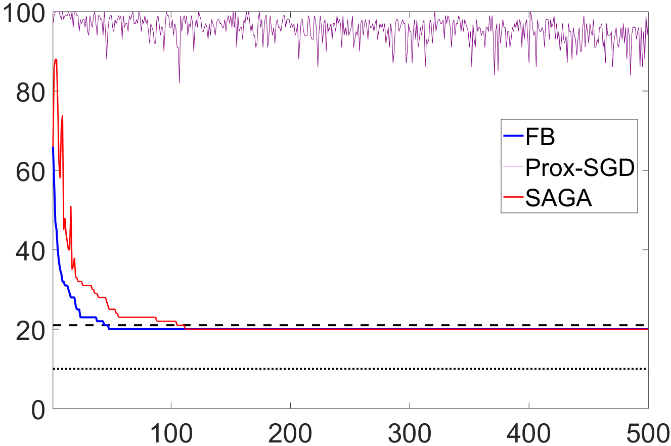
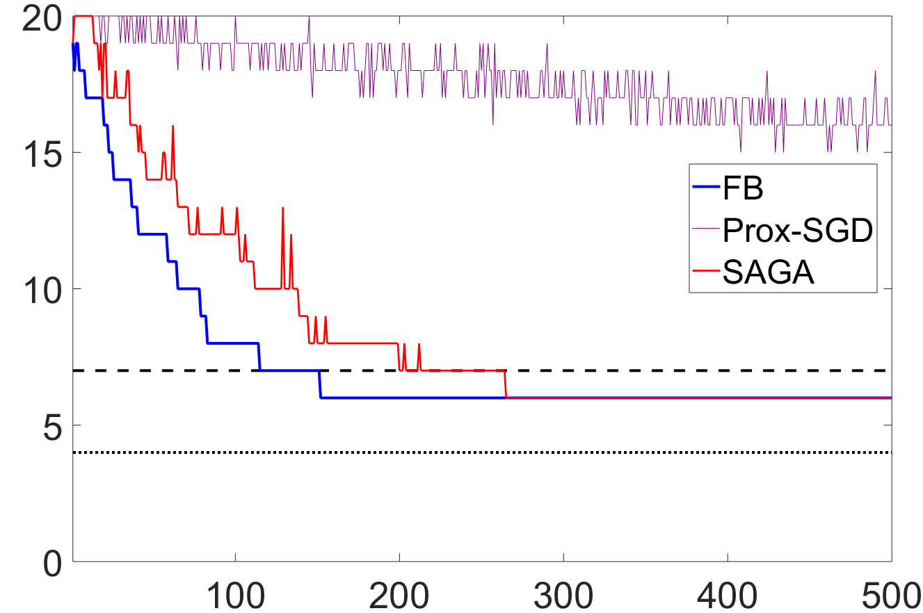
$R=|\!|\cdot|\!|_{1}$	$R=|\!|\cdot|\!|_{*}$

Figure 1: Evolution of $R_{0}(M_{\widehat{w}^{k}})$ along the batches of the FB (blue), Prox-SGD (purple) and SAGA (red) algorithms, applied to solve ($\text{P}_{\lambda,n}$). The black dotted line (resp. black dashed line) indicates the value $R_{0}(M_{w_{0}})$ (resp. the value of $R_{0}(\mathcal{J}_{R^{*}}(M^{*}_{\eta_{0}}))$ ); these are the dimensions of the two extreme strata.

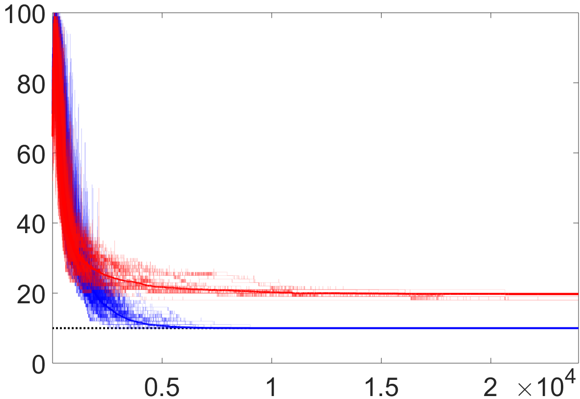
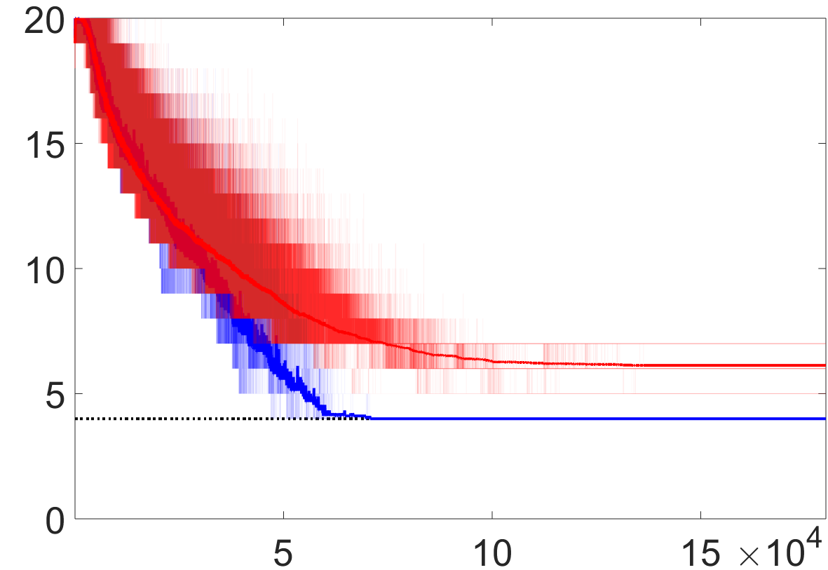
$R=|\!|\cdot|\!|_{1}$	$R=|\!|\cdot|\!|_{*}$

Figure 2: Evolution of $R_{0}(M_{\widehat{w}^{k}})$ along the iterations of SAGA, for problems where $R_{0}(\mathcal{J}_{R^{*}}(M^{*}_{\eta_{0}}))=R_{0}(M_{w_{0}})+\delta$. Blue trajectories correspond to problems for which $\delta=0$, and for red trajectories $\delta=10$ (left) or $3$ (right). The thick lines correspond to averaged trajectories. The black dotted line indicates the value $R_{0}(M_{w_{0}})$.

5 Numerical illustrations for sparse/low-rank regularization

We give some numerical illustrations of our model consistency results for two popular regularizers: the $\ell_{1}$-norm and the nuclear norm. We generate random problem instances and control the low-complexity of the primal-dual pair of strata $(M_{w_{0}},\mathcal{J}_{R^{*}}(M^{*}_{\eta_{0}}))$. The low-complexity of a strata $M_{w}$ (i.e., the level of low-complexity of $w$) is measured by

$$R_{0}(M_{w}) :=|\!|w|\!|_{0}\quad\text{for $R=|\!|\cdot|\!|_{1}$},$$

$$R_{0}(M_{w}) :=\operatorname{rank}(w)\quad\text{for $R=|\!|\cdot|\!|_{*}$}.$$

Observe that $R_{0}$ is well defined, since it does not depend of the choice of $w$ in the strata (see Example 1).

Setup.

The instances are randomly generated as follows. For $R=|\!|\cdot|\!|_{1}$, $w_{0}$ is drawn randomly among sparse vectors with sparsity level $R_{0}(M_{w_{0}})=|\!|w_{0}|\!|_{0}=s$, and we take $(p,n,s,\lambda)=(100,50,10,0.2)$. For $R=|\!|\cdot|\!|_{*}$, $w_{0}$ is drawn randomly among low-rank matrices with rank $R_{0}(M_{w_{0}})=\operatorname{rank}(w_{0})=s$, and we take $(p,n,s,\lambda)=(20\times 20,300,4,0.03)$. The features $(x_{i})_{i=1}^{n}$ are drawn at random in $\mathbb{R}^{p}$ with i.i.d. entries from a zero-mean standard Gaussian distribution. We take $y_{i}$ as $\langle w_{0},x_{i}\rangle$, to which we add a zero-mean white Gaussian noise with standard deviation $10^{-2}$. We compute $\eta_{0}$ with an interior point solver, from which we deduce the upper-bound $R_{0}(\mathcal{J}_{R^{*}}(M^{*}_{\eta_{0}}))$.

FB vs. Prox-SGD vs. SAGA.

First, we compare the deterministic Forward-Backward (FB) algorithm, the Prox-SGD method and SAGA on a simple instance of ($\text{P}_{\lambda,n}$). All algorithms are run with $\alpha_{k}\equiv 1$, and we take $\gamma_{k}\equiv 1.8/L_{n}$ for the FB algorithm, $\gamma_{k}=10/(k+3\times 10^{4})$, and $\gamma_{k}\equiv 1/(3L_{n}^{\prime})$ for SAGA, where $L_{n}$ is defined in ($\text{H}_{\text{A}}$) and $L_{n}^{\prime}:=\max_{i}|\!|x_{i}|\!|^{2}$. Figure 1 depicts the evolution of $R_{0}(M_{\widehat{w}^{k}})$ while running these three algorithms on ($\text{P}_{\lambda,n}$). At each iteration, FB visits all the data at once, while Prox-SGD and SAGA need only one data. To fairly compare these three algorithms, we plot only the iterates at every batch (i.e. all iterates for FB, and one every $n$ iterates for the stochastic algorithms).

As expected, the two stochastic algorithms exhibit an oscillating behaviour. But for SAGA, these oscillations are damped quickly, and the support of $\widehat{w}^{k}$ stabilizes after a finite number of iterations. On the contrary, Prox-SGD suffers from constant variations of the support, and is unable to generate iterates with a sparse support. Another observation is that FB and SAGA identify a support which is larger than the one of $w_{0}$ but below the extended one governed by $\eta_{0}$, which is in agreement with Theorem 2. A natural question is then: if we replace $w_{0}$ by another low-complexity vector, and consider other data, what can be said about the complexity of the obtained solution? This is discussed next.

Randomized experiments for SAGA.

We now focus on SAGA, and look at the strata that its iterates can identify. For the $\ell_{1}$ norm (resp. nuclear norm), we draw 1000 (resp. 200) realizations of $(w_{0},(x_{i},y_{i})_{i=1}^{n})$ exactly as before. For each realization, we compute $\eta_{0}$ with high precision by using a solver. We then select among the realizations those for which $R_{0}(\mathcal{J}_{R^{*}}(M^{*}_{\eta_{0}}))$ belongs exactly to $\{10,20\}$ for the $\ell_{1}$ norm (resp. to $\{4,7\}$ for the nuclear norm), and we apply the SAGA algorithm to these. The evolution of $R_{0}(M_{\widehat{w}^{k}})$ in these cases are plotted in Figure 2.

We see that for the realizations for which $R_{0}(\mathcal{J}_{R^{*}}(M^{*}_{\eta_{0}}))=R_{0}(M_{w_{0}})$ (the blue curves), the algorithm indeed identifies in finite time the stratum where $w_{0}$ belongs. Otherwise, we see that the algorithm often identifies a stratum of the same dimension as that of $R_{0}(\mathcal{J}_{R^{*}}(M^{*}_{\eta_{0}}))$, or sometimes smaller, but which is always larger than $M_{w_{0}}$. These observations are consistent with the predictions of Theorem 2.

6 Conclusion

In this paper, we provided a fine and unified analysis for studying model stability/consistency, when considering empirical risk minimization with a mirror-stratifiable regularizer, and solving it with a stochastic algorithm. We showed that, even in the absence of the irrepresentable condition, the low-complexity of an approximate empirical solution remains controlled by a dual certificate. Moreover, we proposed a general algorithmic framework in which stochastic algorithms inherit almost surely finite activity identification.

Appendix A Supplementary material

This is the supplementary material for the paper Model Consistency for Learning with Mirror-Stratifiable Regularizers. It contains the detailed proofs of the propositions 2 and 3 of which are, as explained in Section 4, the building blocks of our two main results (Theorems 1 and 2). The supplementary is structured in three sections: Section A.1 gathers key technical lemmas; Section A.2 presents the proof of Proposition 2; Section A.3 presents the one of Proposition 3.

We use the same notations here as introduced at the beginning of Section 4. We also introduce what can viewed as the limit of ($\text{P}_{\lambda,n}$) as $n\rightarrow+\infty$:

$$w_{\lambda}\in\underset{w\in\mathbb{R}^{p}}{\operatorname{Argmin}}\;\lambda R(w)+\frac{1}{2}\langle Cw,\,w\rangle-\langle u,\,w\rangle.$$ (9)

For any positive semi-definite matrix $A$, we also note the seminorm $|\!|\cdot|\!|_{A}=\sqrt{\langle A\cdot,\,\cdot\rangle}$.

A.1 Useful technical lemmas

Here we present a few technical lemmas. The first gives us some control on how $\widehat{C}_{n}$ converges to $C$ (resp. $\widehat{u}_{n}$ converges to $u$) when the amount of data $n$ tends to $+\infty$, and the second provides us with some essential compactness on these sequences. The third provides us an important variational characterization of the set to which belongs $\eta_{0}$. Finally, the last Lemma gives a useful estimate between $\widehat{w}_{\lambda,n}$ and $w_{\lambda}$.

Lemma 1.

If $\lambda_{n}\sqrt{n/\log\log n}\to+\infty$ and $\mathbb{E}\left[|\mathrm{\bf y}|^{4}\right]+\mathbb{E}\left[|\!|\mathrm{\bf x}|\!|^{4}\right]<+\infty$, then the following holds almost surely:

1. $\max\{\|\widehat{u}_{n}-u\|,\|\widehat{C}_{n}-C\|\}=o(\lambda_{n})$,

2. for $n$ large enough, $\operatorname{Im}\widehat{C}_{n}=\operatorname{Im}C$,

3. $\widehat{C}_{n}^{\dagger}\rightarrow C^{\dagger}$ as $n\to+\infty$.

Proof.

It can be seen (use the Young inequality) that

$$\mathbb{E}\left[|\!|\mathbb{xy}|\!|^{2}\right] = \mathbb{E}\left[|\mathrm{\bf y}|^{2}|\!|\mathrm{\bf x}|\!|^{2}\right]$$

$$\leqslant \frac{1}{2}\mathbb{E}\left[|\mathrm{\bf y}|^{4}\right]+\frac{1}{2}\mathbb{E}\left[|\!|\mathrm{\bf x}|\!|^{4}\right]<+\infty$$

$$\text{ and }\mathbb{E}\left[|\!|\mathbb{xx}^{\top}|\!|^{2}\right] = \mathbb{E}\left[|\!|\mathbb{x}|\!|^{4}\right]<+\infty.$$

We are then in a position to invoke the law of iterated logarithm (Van der Vaart,, 1998, Proposition 2.26) to obtain that, with probability 1,

$$r_{n}:=\max\{\|\widehat{u}_{n}-u\|,\|\widehat{C}_{n}-C\|\}=O\left(n^{-1/2}\sqrt{{\log\log n}}\right).$$

Our assumption that $\lambda_{n}\sqrt{n/\log\log n}\to+\infty$ then entails item (i).

We now turn to item (ii). Consider $w\in\operatorname{Ker}C$; it verifies by definition $\mathbb{E}_{\rho}[\mathrm{\bf x}\langle\mathrm{\bf x},w\rangle]=0$. By taking the scalar product of this equality with $w$, we see that $(\forall x{~{}\sim~{}}\rho)$,   $\mathbb{P}(\langle x,w\rangle=0)=1.$ Let ($w_{1},...,w_{d}$) be a basis of $\operatorname{Ker}C$, where $d=\dim(\ker C)$. Then we deduce that $(\forall x{~{}\sim~{}}\rho)$,   $\mathbb{P}((\forall i\in\{1,\ldots,d\})\ \langle x,w_{i}\rangle=0)=1$. In other words, $x\in(\operatorname{Ker}C)^{\perp}$ a.s., or, equivalently:

$$(\forall x\underset{i.i.d.}{\sim}\rho)\quad\mathbb{P}(x\in\operatorname{Im}C)=1.$$ (10)

Now, observe that $\operatorname{Im}\widehat{C}_{n}=\operatorname{Im}\left(\{x_{i}\}_{i=1}^{n}\right)$, so the following implication holds:

$$\left[(\forall i\in\{1,\ldots,n\})\ x_{i}\in\operatorname{Im}C\right]\Rightarrow\operatorname{Im}\widehat{C}_{n}\subset\operatorname{Im}C.$$ (11)

Since the $x_{i}$ are drawn i.i.d. from $\rho$, and are in finite number, we can combine (10) and (11) to obtain that

$$\mathbb{P}(\operatorname{Im}\widehat{C}_{n}\subset\operatorname{Im}C) \geqslant \mathbb{P}((\forall i\in\{1,\ldots,n\})\ x_{i}\in\operatorname{Im}C)$$

$$= \prod_{i=1}^{n}\mathbb{P}(x_{i}\in\operatorname{Im}C)=1.$$

We deduce then that $\operatorname{Im}\widehat{C}_{n}\subset\operatorname{Im}C$ a.s., from which we get that $\operatorname{rank}\widehat{C}_{k}\leqslant\operatorname{rank}C$ a.s. This, together with lower semi-continuity of the rank, yields that with probability 1,

$$\operatorname{rank}(C)\leqslant\liminf\limits_{k\to+\infty}\operatorname{rank}(\widehat{C}_{k}) \leqslant \limsup\limits_{k\to+\infty}\operatorname{rank}(\widehat{C}_{k})$$

$$\leqslant \operatorname{rank}C\ \,$$

meaning that $\operatorname{rank}(\widehat{C}_{k})\to\operatorname{rank}(C)$ a.s. Because the rank takes only discrete values, this means that $\operatorname{rank}\widehat{C}_{k}=\operatorname{rank}C$ a.s. for all $k$ large enough. We can then trivially deduce from the inclusion $\operatorname{Im}\widehat{C}_{k}\subset\operatorname{Im}C$ a.s., that the equality $\operatorname{Im}\widehat{C}_{k}=\operatorname{Im}C$ holds a.s. for $k$ large enough.

Assertion (iii) follows from (ii) and (Stewart,, 1977, Theorem 3.3). ∎

Lemma 2.

Assume that ($\text{H}_{\text{M}}$) holds, and

• $\operatorname{Im}\widehat{C}_{n}=\operatorname{Im}C$ for $n$ large enough,

• $\sup_{n\in\mathbb{N}}\widehat{C}_{n}^{\dagger}<+\infty$.

Then, the sequences $(\widehat{w}_{\lambda_{n},n})_{n\in\mathbb{N}}$ and $(w_{\lambda_{n}})_{n\in\mathbb{N}}$ are bounded.

Proof.

Introduce $f_{\lambda}(w):=R(w)+(1/2\lambda)|\!|Cw-u|\!|^{2}_{C^{\dagger}}$ and $f_{\lambda,n}(w):=R(w)+(1/2\lambda)|\!|\widehat{C}_{n}w-\widehat{u}_{n}|\!|^{2}_{\widehat{C}_{n}^{\dagger}}$ which, by definition, verify

$$w_{\lambda_{n}}\in\operatorname{Argmin}f_{\lambda_{n}}\text{ and }\widehat{w}_{\lambda_{n},n}\in\operatorname{Argmin}f_{\lambda_{n},n}.$$

Define $\overline{\lambda}:=\sup_{n}\lambda_{n}>0$, and use the optimality of $\widehat{w}_{\lambda_{n},n}$ to derive

$$f_{\overline{\lambda},n}(\widehat{w}_{\lambda_{n},n})\leqslant f_{\lambda_{n},n}(\widehat{w}_{\lambda_{n},n})\leqslant f_{n}(w_{0})$$

By making use of Lemma 1.(iii) and Lemma 1.(i), we have the bound

$$f_{n}(w_{0}) \leqslant R(w_{0})+\frac{|\!|\widehat{C}_{n}^{\dagger}|\!|}{2\lambda_{n}}|\!|\widehat{C}_{n}w_{0}-\widehat{u}_{n}|\!|^{2},$$

$$\leqslant R(w_{0})+O\left(\frac{|\!|\widehat{C}_{n}-C|\!|+|\!|u-\widehat{u}_{n}|\!|}{\lambda_{n}}\right)^{2},$$

$$\leqslant R(w_{0})+o(1).$$

We can make a similar reasoning on the sequence $(w_{\lambda_{n}})_{n\in\mathbb{N}}$, and deduce that

$$f_{\overline{\lambda}}(w_{\lambda_{n}})\leqslant R(w_{0})+o(1),$$ (12)

$$\text{ and }f_{\overline{\lambda},n}(\widehat{w}_{\lambda_{n},n})\leqslant R(w_{0})+o(1).$$ (13)

To prove the boundedness of $(\widehat{w}_{\lambda_{n},n})_{n\in\mathbb{N}}$ and $(w_{\lambda_{n}})_{n\in\mathbb{N}}$, we will use arguments relying on the notion of asymptotic or recession function; see (Bauschke and Combettes,, 2011, Definition 10.32) for a definition. Define $f_{0}(w):=R(w)+\iota_{\{u\}}(Cw)$, where $\iota_{\{u\}}$ is the indicator function of the singleton $\{u\}$. The hypothesis ($\text{H}_{\text{M}}$) indicates that $\operatorname{argmin}f_{0}=\{w_{0}\}$, so in particular $\operatorname{argmin}f_{0}$ is compact. We can then invoke (Auslender and Teboulle,, 2003, Proposition 3.1.2 and 3.1.3) to deduce that $f_{0}^{\infty}(w)>0$ for all $w\in\mathbb{R}^{p}\setminus\{0\}$, where $f_{0}^{\infty}$ is the recession function of $f_{0}$. From the sum rule (Auslender and Teboulle,, 2003, Proposition 2.6.1), we deduce that $f_{0}^{\infty}=R^{\infty}+(\iota_{\{u\}}\circ C)^{\infty}$. Moreover, we know from ($\text{H}_{\text{M}}$) that $u\in\operatorname{Im}C$, so we can use (Auslender and Teboulle,, 2003, Proposition 2.6.1) to get $(\iota_{\{u\}}\circ C)^{\infty}=\iota_{\{0\}}\circ C=\iota_{\operatorname{Ker}C}$. We deduce from all this that $R^{\infty}(w)>0$ for all $w\in\operatorname{Ker}C\setminus\{0\}$, which can be equivalently reformulated as

$$\operatorname{Ker}R^{\infty}\cap\operatorname{Ker}C=\{0\}.$$ (14)

Let us start with the boundedness of $(w_{\lambda_{n}})_{n\in\mathbb{N}}$. Combining (Auslender and Teboulle,, 2003, Proposition 2.6.1), (Auslender and Teboulle,, 2003, Example 2.5.1) and the fact that $u\in\operatorname{Im}C$, the recession function of $f_{\overline{\lambda}}$ reads $f_{\overline{\lambda}}^{\infty}(w)=R^{\infty}(w)$ if $w\in\ker C$ and $+\infty$ otherwise. Thus, (14) is equivalent to $f_{\overline{\lambda}}^{\infty}(w)>0$ for all $w\neq 0$. This is equivalent to saying that $f_{\overline{\lambda}}$ is level-bounded (see (Auslender and Teboulle,, 2003, Proposition 3.1.3)), from which we deduce boundedness of $(w_{\lambda_{n}})_{n\in\mathbb{N}}$ via (12) and (13).

We now turn on $(\widehat{w}_{\lambda_{n},n})_{n\in\mathbb{N}}$. We write $\widehat{u}_{n}=C\widehat{p}_{n}$ since $\widehat{u}_{n}\in\operatorname{Im}\widehat{C}_{n}\subset\operatorname{Im}C$. We first observe that (12) and (13) can be rewritten as:

$$\frac{1}{2\overline{\lambda}}|\!|\widehat{C}_{n}(\widehat{w}_{\lambda_{n},n}-\widehat{p}_{n})|\!|^{2}_{\widehat{C}_{n}^{\dagger}}+R(\widehat{w}_{\lambda_{n},n})\leqslant R(w_{0})+o(1).$$

Let $V_{n}\operatorname{diag}(s_{n,i})V_{n}^{\top}$ be a (reduced) eigendecomposition of $\widehat{C}_{n}$. By our assumptions, we have $\underline{s}:=\inf_{n,1\leqslant i\leqslant r}s_{n,i}=\big{(}\sup_{n}|\!|\widehat{C}_{n}|\!|\big{)}^{-1}>0$. In addition, the columns of $V_{n}$ form an orthonormal basis of $\operatorname{Im}C$ for $n$ large enough. Thus, for all such $n$, we have

$$\underline{s}|\!|\operatorname{proj}_{\operatorname{Im}C}(\widehat{w}_{\lambda_{n},n}-\widehat{p}_{n})|\!|^{2}$$

$$= \underline{s}|\!|V_{n}^{\top}(\widehat{w}_{\lambda_{n},n}-\widehat{p}_{n})|\!|^{2}$$

$$\leqslant \sum_{i=1}^{r}s_{n,i}|\langle v_{n,i},\,\widehat{w}_{\lambda_{n},n}-\widehat{p}_{n}\rangle|^{2}$$

$$= \langle\widehat{C}_{n}(\widehat{w}_{\lambda_{n},n}-\widehat{p}_{n}),\,\widehat{w}_{\lambda_{n},n}-\widehat{p}_{n}\rangle$$

$$= |\!|\widehat{C}_{n}(\widehat{w}_{\lambda_{n},n}-\widehat{p}_{n})|\!|^{2}_{\widehat{C}_{n}^{\dagger}}.$$

Altogether, we get the bound

$$\frac{\underline{s}}{2\overline{\lambda}}|\!|\operatorname{proj}_{\operatorname{Im}C}(\widehat{w}_{\lambda_{n},n}-\widehat{p}_{n})|\!|^{2}+R(\widehat{w}_{\lambda_{n},n})\leqslant R(w_{0})+o(1)$$

for $n$ sufficiently large. Arguing as above, the recession function of $g:=\frac{\underline{s}}{2\overline{\lambda}}|\!|\cdot-\widehat{p}_{n}|\!|^{2}\circ\operatorname{proj}_{\operatorname{Im}C}+R$ is again $g^{\infty}(w)=R^{\infty}(w)$ if $w\in\ker C$ and $+\infty$ otherwise, independently of $\widehat{p}_{n}$. Our assumption plugged into (Auslender and Teboulle,, 2003, Proposition 3.1.3) entails that $g$ is level-bounded and thus boundedness for $(\widehat{w}_{\lambda_{n},n})_{n\in\mathbb{N}}$. ∎

Lemma 3.

Assume that ($\text{H}_{\text{M}}$) holds. Then

$$\underset{\eta\in\operatorname{Im}C}{\operatorname{Argmin}}\;R^{*}(\eta)-\langle C^{\dagger}u,\,\eta\rangle=\partial R(w_{0})\cap\operatorname{Im}C.$$

Proof.

Using (Bauschke and Combettes,, 2011, Proposition 13.23 & Theorem 15.27), one can check that problem

$$\underset{\eta\in\operatorname{Im}C}{\min}\;R^{*}(\eta)-\langle C^{\dagger}u,\,\eta\rangle$$

is the Fenchel dual of ($\text{P}_{0}$). Moreover, $(w^{\star},\eta^{\star})$ is a primal-dual (Kuhn-Tucker) optimal pair if and only if

$$\begin{pmatrix}w^{\star}\\ \eta^{\star}\end{pmatrix}\in\begin{pmatrix}C^{\dagger}u+\ker C\\ \partial R(w^{\star})\cap\operatorname{Im}C\end{pmatrix}.$$

As we assumed in ($\text{H}_{\text{M}}$) that $w_{0}$ is the unique minimizer of ($\text{P}_{0}$), the claimed identity follows. ∎

Lemma 4.

Let $n\in\mathbb{N}$ and assume that $\operatorname{Im}\widehat{C}_{n}\subset\operatorname{Im}C$. Denote $r_{n}:=\max\{|\!|\widehat{u}_{n}-u|\!|,|\!|\widehat{C}_{n}-C|\!|\}$. Then,

$$|\!|C(\widehat{w}_{\lambda,n}-w_{\lambda})|\!|\leqslant(|\!|C|\!||\!|C^{\dagger}|\!|)^{1/2}(1+|\!|\widehat{w}_{\lambda,n}|\!|)r_{n}.$$

Proof.

The first-order optimality conditions for both $\widehat{w}_{\lambda,n}$ and $w_{\lambda}$ yield

$$\left\{\begin{array}[]{rl}0&\in\lambda\partial R(\widehat{w}_{\lambda,n})+\widehat{C}_{n}\widehat{w}_{\lambda,n}-\widehat{u}_{n}\\ 0&\in\lambda\partial R(w_{\lambda})+Cw_{\lambda}-u.\end{array}\right.$$

In view of monotonicity of $\partial R$, we deduce that

$$0\leqslant\langle\widehat{u}_{n}-u+Cw_{\lambda}-\widehat{C}_{n}\widehat{w}_{\lambda,n},\,\widehat{w}_{\lambda,n}-w_{\lambda}\rangle.$$

Rearranging the terms, we get

$$\langle C(\widehat{w}_{\lambda,n}-w_{\lambda}),\,\widehat{w}_{\lambda,n}-w_{\lambda}\rangle$$

$$\leqslant \langle\widehat{u}_{n}-u+(C-\widehat{C}_{n})\widehat{w}_{\lambda,n},\,\widehat{w}_{\lambda,n}-w_{\lambda}\rangle.$$

By virtue of standard properties of the Moore-Penrose pseudo-inverse and the fact that $\widehat{u}_{n}-u$ and $C-\widehat{C}_{n}$ both live in $\operatorname{Im}C\supset\operatorname{Im}\widehat{C}_{n}$, we obtain

$$\langle C^{\dagger}(C\widehat{w}_{\lambda,n}-Cw_{\lambda}),\,C\widehat{w}_{\lambda,n}-Cw_{\lambda}\rangle$$

$$\leqslant \langle C^{\dagger}(\widehat{u}_{n}-u+(C-\widehat{C}_{n})\widehat{w}_{\lambda,n}),\,C\widehat{w}_{\lambda,n}-Cw_{\lambda}\rangle.$$

Applying the Cauchy-Schwarz and triangle inequalities, we arrive at

$$|\!|C\widehat{w}_{\lambda,n}-Cw_{\lambda}|\!|_{C^{\dagger}}$$

$$\leqslant |\!|\widehat{u}_{n}-u|\!|_{C^{\dagger}}+|\!|(C-\widehat{C}_{n})\widehat{w}_{\lambda,n}|\!|_{C^{\dagger}}$$

$$\leqslant |\!|C^{\dagger}|\!|^{1/2}\left(|\!|\widehat{u}_{n}-u|\!|+|\!|C-\widehat{C}_{n}|\!||\!|\widehat{w}_{\lambda,n}|\!|\right)$$

$$\leqslant |\!|C^{\dagger}|\!|^{1/2}(1+|\!|\widehat{w}_{\lambda,n}|\!|)r_{n}.$$

On the left side of this inequality, we exploit the fact that $|\!|C|\!|^{-1}$ is the smallest nonzero eigenvalue of $C^{\dagger}$ on $\operatorname{Im}(C)$ to conclude

$$|\!|C\widehat{w}_{\lambda,n}-Cw_{\lambda}|\!|_{C^{\dagger}} \leqslant |\!|C|\!|^{1/2}|\!|C\widehat{w}_{\lambda,n}-Cw_{\lambda}|\!|_{C^{\dagger}}$$

$$\leqslant (|\!|C|\!||\!|C^{\dagger}|\!|)^{1/2}(1+|\!|\widehat{w}_{\lambda,n}|\!|)r_{n}.$$

∎

A.2 Proof of Proposition 2

Convergence of the primal variable.

To lighten notations, we will write $\widehat{w}_{n}:=\widehat{w}_{\lambda_{n},n}$. From Lemma 2 we know that $(\widehat{w}_{n})_{n\in\mathbb{N}}$ is bounded a.s., so it admits a cluster point, say $w^{\star}$. Let $\widehat{w}_{n}$ be a subsequence (we do not relabel for simplicity) converging a.s. to $w^{\star}$. Now, let $\varepsilon_{n}:=\widehat{u}_{n}-\widehat{C}_{n}w_{0}$, for which we know that both $\varepsilon_{n}$ and $\varepsilon_{n}/\lambda_{n}$ are $o(1)$, thanks to Lemma 1(i) and the fact that $u=Cw_{0}$. From the optimality of $\widehat{w}_{n}$, we obtain

$$\lambda_{n}R(\widehat{w}_{n})+\frac{1}{2}\langle\widehat{C}_{n}\widehat{w}_{n},\widehat{w}_{n}\rangle-\langle\widehat{u}_{n},\widehat{w}_{n}\rangle$$

$$\leqslant \lambda_{n}R(w_{0})+\frac{1}{2}\langle\widehat{C}_{n}w_{0},w_{0}\rangle-\langle\widehat{u}_{n},w_{0}\rangle,$$

which can be equivalently rewritten as

$$\frac{1}{2}\langle\widehat{C}_{n}(\widehat{w}_{n}-w_{0}),\widehat{w}_{n}-w_{0}\rangle-\langle\widehat{w}_{n}-w_{0},\varepsilon_{n}\rangle\hskip 28.45274pt$$

$$\leqslant \lambda_{n}(R(w_{0})-R(\widehat{w}_{n})).$$

Passing to the limit in (A.2) and using the fact that $R$ is bounded from below, we obtain

$$\langle C(w^{\star}-w_{0}),\,w^{\star}-w_{0}\rangle=0\text{ a.s. },$$

or equivalently, that $Cw^{\star}=Cw_{0}=u$ a.s. since $C$ is positive semi-definite. In addition, as $\widehat{C}_{n}$ is also positive semi-definite, so we can rewrite (A.2) as

$$R(\widehat{w}_{n})\leqslant R(w_{0})+\langle\widehat{w}_{n}-w_{0},\,\frac{\varepsilon_{n}}{\lambda_{n}}\rangle.$$ (17)

Passing to the limit in (17), using lower-semicontinuity of $R$ and that $\varepsilon_{n}/\lambda_{n}=o(1)$ a.s., we arrive at

$$R(w^{\star})\leqslant\liminf_{n}R(\widehat{w}_{n})\leqslant\limsup_{n}R(\widehat{w}_{n})\leqslant R(w_{0})\quad a.s.$$

Clearly $R(w^{\star})\leqslant R(w_{0})$ and $w^{\star}$ obeys the constraint $Cw^{\star}=u$, which implies that $w^{\star}$ is a solution of ($\text{P}_{0}$) a.s. But since this problem has a unique solution, $w_{0}$, by assumption ($\text{H}_{\text{M}}$), we conclude that $w^{\star}=w_{0}$ a.s. This being true for any a.s. cluster point means that $\widehat{w}_{n}\to w_{0}$ as $n\to+\infty$ a.s.

Convergence of the dual variable.

Here we omit systematically mentioning that the bounds and convergence we obtain hold almost surely.

It can be verified, using for instance (Bauschke and Combettes,, 2011, Proposition 13.23 & Theorem 15.27), that the Fenchel dual problem of ($\text{P}_{\lambda,n}$) is

$$\{\widehat{\eta}_{\lambda,n}\}:=\underset{\eta\in\operatorname{Im}\widehat{C}_{n}}{\operatorname{Argmin}}\;R^{*}(\eta)+\frac{\lambda}{2}\langle\widehat{C}_{n}^{\dagger}\eta,\eta\rangle-\langle\widehat{C}_{n}^{\dagger}\widehat{u}_{n},\eta\rangle.$$ (18)

For any fixed $\lambda>0$, we also introduce its limit problem, as $n\to+\infty$ (which is the dual of (9)):

$$\{\eta_{\lambda}\}:=\underset{\eta\in\operatorname{Im}C}{\operatorname{Argmin}}\;R^{*}(\eta)+\frac{\lambda}{2}\langle C^{\dagger}\eta,\eta\rangle-\langle C^{\dagger}u,\eta\rangle.$$ (19)

Both problems are strongly convex thanks to positive semi-definiteness of $\widehat{C}_{n}$ and $C$, hence uniqueness of the corresponding dual solutions $\widehat{\eta}_{\lambda,n}$ and $\eta_{\lambda}$. Moreover, from the primal-dual extremality relationships, see (Bauschke and Combettes,, 2011, Proposition 26.1.iv.b), $\widehat{\eta}_{\lambda,n}$ and $\eta_{\lambda}$ can be recovered from the corresponding primal solutions as

$$\widehat{\eta}_{\lambda,n}:=\frac{\widehat{u}_{n}-\widehat{C}_{n}\widehat{w}_{\lambda,n}}{\lambda}\quad\text{and}\quad\eta_{\lambda}:=\frac{u-Cw_{\lambda}}{\lambda}.$$ (20)

In what follows, we prove that $\widehat{\eta}_{n}$ converges to $\eta_{0}$ when $n\to+\infty$. To lighten notation, we will denote $r_{n}:=\max\{\|\widehat{u}_{n}-u\|,\|\widehat{C}_{n}-C\|\}$, and note $\widehat{\eta}_{n}=\widehat{\eta}_{\lambda_{n},n}$. We have

$$|\!|\widehat{\eta}_{n}-\eta_{0}|\!|\leqslant|\!|\widehat{\eta}_{n}-\eta_{\lambda_{n}}|\!|+|\!|\eta_{\lambda_{n}}-\eta_{0}|\!|.$$ (21)

By using (20) and the definition of $r_{n}$, we write

$$|\!|\widehat{\eta}_{n}-\eta_{\lambda_{n}}|\!| = \Big{|}\!\Big{|}\frac{\widehat{u}_{n}-u}{\lambda_{n}}+\frac{Cw_{\lambda_{n}}-\widehat{C}_{n}\widehat{w}_{n}}{\lambda_{n}}\Big{|}\!\Big{|}$$

$$\leqslant O\left(\frac{r_{n}}{\lambda_{n}}\right)+\Big{|}\!\Big{|}\frac{Cw_{\lambda_{n}}-\widehat{C}_{n}\widehat{w}_{n}}{\lambda_{n}}\Big{|}\!\Big{|}.$$

The second term on the right hand side can also be bounded as

$$\Big{|}\!\Big{|}\frac{Cw_{\lambda_{n}}-\widehat{C}_{n}\widehat{w}_{n}}{\lambda_{n}}\Big{|}\!\Big{|} = \Big{|}\!\Big{|}\frac{C(w_{\lambda_{n}}-\widehat{w}_{n})}{\lambda_{n}}+\frac{C\widehat{w}_{n}-\widehat{C}_{n}\widehat{w}_{n}}{\lambda_{n}}\Big{|}\!\Big{|}$$

$$\leqslant \Big{|}\!\Big{|}\frac{C(w_{\lambda_{n}}-\widehat{w}_{n})}{\lambda_{n}}\Big{|}\!\Big{|}+|\!|\widehat{w}_{n}|\!|\frac{r_{n}}{\lambda_{n}}$$

$$= O\left(\frac{r_{n}}{\lambda_{n}}\right),$$

where we used Lemma 4, and Lemma 2 with Lemma 1 in the last inequality. Combining the above inequalities with the fact that $r_{n}=o(\lambda_{n})$ by Lemma 1.(i), we obtain

$$|\!|\widehat{\eta}_{n}-\eta_{\lambda_{n}}|\!|=O\left(\frac{r_{n}}{\lambda_{n}}\right)\overset{n\to+\infty}{\longrightarrow}0.$$ (22)

It remains now to prove that $\eta_{\lambda}$ converges to $\eta_{0}$ when $\lambda\to 0$. To do so, we start by using optimality of $\eta_{\lambda}$ and $\eta_{0}$ for problems (19) and ($\text{D}_{\text{0}}$), together with Lemma 3, to write

$$R^{*}(\eta_{\lambda})+\frac{\lambda}{2}\langle C^{\dagger}\eta_{\lambda},\eta_{\lambda}\rangle-\langle C^{\dagger}u,\eta_{\lambda}\rangle$$

$$\leqslant R^{*}(\eta_{0})+\frac{\lambda}{2}\langle C^{\dagger}\eta_{0},\eta_{0}\rangle-\langle C^{\dagger}u,\eta_{0}\rangle$$

$$\leqslant R^{*}(\eta_{\lambda})+\frac{\lambda}{2}\langle C^{\dagger}\eta_{0},\eta_{0}\rangle-\langle C^{\dagger}u,\eta_{\lambda}\rangle,$$

from which we deduce that

$$\langle C^{\dagger}\eta_{\lambda},\eta_{\lambda}\rangle\leqslant\langle C^{\dagger}\eta_{0},\eta_{0}\rangle.$$ (24)

Since $\eta_{\lambda}\in\operatorname{Im}C=(\ker C^{\dagger})^{\perp}$ (see (19)), we can infer from (24) that $(\eta_{\lambda})_{\lambda>0}$ is bounded. Let $\eta^{\star}$ be any cluster point of this net, and let us verify that $\eta^{\star}$ must be equal to $\eta_{0}$. First, passing to the limit in (24) shows that

$$\langle C^{\dagger}\eta^{\star},\eta^{\star}\rangle\leqslant\langle C^{\dagger}\eta_{0},\eta_{0}\rangle.$$ (25)

Second, taking the limit in (A.2) and using lower semi-continuity of $R^{*}$, we get

$$R^{*}(\eta^{\star})-\langle C^{\dagger}u,\eta^{\star}\rangle$$

$$\leqslant \liminf_{\lambda\to 0}R^{*}(\eta_{\lambda})+\frac{\lambda}{2}\langle C^{\dagger}\eta_{\lambda},\eta_{\lambda}\rangle-\langle C^{\dagger}u,\eta_{\lambda}\rangle\hskip 28.45274pt$$

$$\leqslant \lim_{\lambda\to 0}R^{*}(\eta_{0})+\frac{\lambda}{2}\langle C^{\dagger}\eta_{0},\eta_{0}\rangle-\langle C^{\dagger}u,\eta_{0}\rangle$$

$$= R^{*}(\eta_{0})-\langle C^{\dagger}u,\eta_{0}\rangle.$$

From $\eta_{\lambda}\in\operatorname{Im}C$ we know that $\eta^{\star}\in\operatorname{Im}C$ as well, so we can then deduce from (A.2) and Lemma 3 that

$$\eta^{\star}\in\partial R(w_{0})\cap\operatorname{Im}C.$$ (27)

Putting together (25) and (27) shows that $\eta^{\star}$ is a solution of ($\text{D}_{\text{0}}$), hence $\eta^{\star}=\eta_{0}$ by uniqueness of $\eta_{0}$. This being true for any cluster point shows convergence of $\eta_{\lambda}$ to $\eta_{0}$.

A.3 Proof of Proposition 3

We use here the notations $h_{n}$ and $\widehat{\xi}^{k}$ introduced in Section 4, and we read directly from hypothesis ($\text{H}_{\text{A}}$) that $\widehat{d}^{k}=\nabla h_{n}(\widehat{w}^{k})+\widehat{\xi}^{k}$, $\mathbb{E}\left[\widehat{\xi}^{k}|\mathcal{F}_{k}\right]=0,\ \mathbb{E}\left[\|\widehat{\xi}^{k}\|^{2}|\mathcal{F}_{k}\right]\leqslant\sigma_{k}^{2}\text{ and }\widehat{\xi}^{k}\text{ converges a.s. to }0.$

Let us start by showing that $\widehat{w}^{k}$ converges to $\widehat{w}_{\lambda_{n},n}$. For this, let $w$ be any solution of ($\text{P}_{\lambda,n}$). We can write, using standard identities (e.g. (Bauschke and Combettes,, 2011, Corollary 2.14)), that

$$|\!|\widehat{w}^{k+1}-w|\!|^{2}$$

$$= |\!|(1-\alpha_{k})(\widehat{w}^{k}-w)+\alpha_{k}(\widehat{z}^{k}-w)|\!|^{2}$$

$$= (1-\alpha_{k})|\!|\widehat{w}^{k}-w|\!|^{2}+\alpha_{k}|\!|\widehat{z}^{k}-w|\!|^{2}$$

$$-\alpha_{k}(1-\alpha_{k})|\!|\widehat{z}^{k}-\widehat{w}^{k}|\!|^{2}.$$

Since $w$ is a solution of ($\text{P}_{\lambda,n}$), it is a fixed point for the operator $\operatorname{prox}_{\lambda_{n}\gamma_{k}R}\circ(\mathrm{Id}-\gamma_{k}\nabla h_{n})$ for any $k\in\mathbb{N}$. Use then the definition of $\widehat{z}^{k}$ together with the nonexpansiveness of the proximal mapping to obtain

$$|\!|\widehat{z}^{k}-w|\!|^{2} \leqslant|\!|\widehat{w}^{k}-w+\gamma_{k}(\nabla h_{n}(w)-\nabla h_{n}(\widehat{w}^{k})-\xi_{k})|\!|^{2}$$

$$\leqslant|\!|\widehat{w}^{k}-w\|^{2}+\gamma_{k}^{2}\|\nabla h_{n}(w)-\nabla h_{n}(\widehat{w}^{k})-\xi_{k}|\!|^{2}$$

$$\hskip 8.5359pt+2\gamma_{k}\langle\widehat{w}^{k}-w,\,\nabla h_{n}(w)-\nabla h_{n}(\widehat{w}^{k})-\xi_{k}\rangle.$$

Taking the conditional expectation w.r.t. $\mathcal{F}_{k}$ in the above inequality, and using the assumptions $\mathbb{E}(\xi_{k}|\mathcal{F}_{k})=0$ and $\mathbb{E}(\|\xi_{k}\|^{2}|\mathcal{F}_{k})\leqslant\sigma_{k}^{2}$, leads to

$$\mathbb{E}(|\!|\widehat{z}^{k}-w|\!|^{2}|\mathcal{F}_{k})$$

$$\leqslant |\!|\widehat{w}^{k}-w|\!|^{2}+\gamma_{k}^{2}|\!|\nabla h_{n}(w)-\nabla h_{n}(\widehat{w}^{k})|\!|^{2}+\gamma_{k}^{2}\sigma_{k}^{2}$$

$$+2\gamma_{k}\langle\widehat{w}^{k}-w,\,\nabla h_{n}(w)-\nabla h_{n}(\widehat{w}^{k})\rangle.$$

Since $\nabla h_{n}$ is $1/L$-cocoercive, we obtain

$$\begin{array}[]{lll}&&\mathbb{E}(|\!|\widehat{z}^{k}-w|\!|^{2}|\mathcal{F}_{k})\\ &\leqslant&|\!|\widehat{w}^{k}-w|\!|^{2}+\gamma_{k}^{2}\sigma_{k}^{2}\\ &&-\gamma_{k}(2/L-\gamma_{k})|\!|\nabla h_{n}(w)-\nabla h_{n}(\widehat{w}^{k})|\!|^{2}\end{array}$$

After taking the conditional expectation in (A.3) and combining with the last inequality, we obtain

$$\mathbb{E}(|\!|\widehat{w}^{k+1}-w|\!|^{2}|\mathcal{F}_{k})$$

$$\leqslant |\!|\widehat{w}^{k}-w|\!|^{2}+\alpha_{k}\gamma_{k}^{2}\sigma_{k}^{2}$$

$$-\gamma_{k}(2/L-\gamma_{k})|\!|\nabla h_{n}(w)-\nabla h_{n}(\widehat{w}^{k})|\!|^{2}$$

$$-\alpha_{k}(1-\alpha_{k})\mathbb{E}(|\!|\widehat{z}^{k}-\widehat{w}^{k}|\!|^{2}|\mathcal{F}_{k}).$$

The inequality above means that $(\widehat{w}^{k})_{k\in\mathbb{N}}$ is a stochastic quasi-Féjer sequence, and hypothesis ($\text{H}_{\text{A}}$) allows us to use invoke (Combettes and Pesquet,, 2015, Proposition 2.3), from which we deduce that $(\widehat{w}^{k})_{k\in\mathbb{N}}$ is bounded a.s. Thus $\widehat{w}^{k}$ has a cluster point. Let $\bar{w}$ be a sequential cluster point of $(\widehat{w}^{k})_{k\in\mathbb{N}}$, and $\widehat{w}^{k}$ be a subsequence (that we do not relabel for simplicity) that converges a.s. to $\bar{w}$. Recalling (8) and (7), and in view of assumption ($\text{H}_{\text{A}}$) and continuity of the gradient, we deduce that

$$\widehat{v}^{k}\to-\nabla h_{n}(\bar{w})\quad\text{and}\quad\widehat{z}^{k}\to\bar{w}\quad a.s.$$

Since $(\widehat{z}^{k},\widehat{v}^{k})\in\operatorname{gph}(\lambda_{n}\partial R)$ and $\lambda_{n}\partial R$ is maximally monotone, we conclude that $0\in\nabla h_{n}(\bar{w})+\lambda_{n}\partial R(\bar{w})$, i.e., $\bar{w}$ is minimizer of ($\text{P}_{\lambda,n}$). Since this is true for any cluster point, we invoke (Combettes and Pesquet,, 2015, Proposition 2.3(iv)) which yields that $\widehat{w}^{k}$ converges a.s. to a minimizer of ($\text{P}_{\lambda,n}$). Using again (7), we see that $\widehat{z}^{k}$ converges a.s. to this same minimizer.

References

• A. Defazio and Lacoste-Julien, (2014) A. Defazio, F. B. and Lacoste-Julien, S. (2014). Saga: A fast incremental gradient method with support for non-strongly convex composite objectives. In NIPS.
• Amelunxen et al., (2014) Amelunxen, D., Lotz, M., McCoy, M. B., and Tropp, J. A. (2014). Living on the edge: Phase transitions in convex programs with random data. Information and Inference: A Journal of the IMA, 3(3):224–294.
• Atchadé et al., (2017) Atchadé, Y. F., Fort, G., and Moulines, E. (2017). On perturbed proximal gradient algorithms. J. Mach. Learn. Res, 18(1):310–342.
• Auslender and Teboulle, (2003) Auslender, A. and Teboulle, M. (2003). Asymptotic Cones and Functions in Optimization and Variational Inequalities. Springer.
• (5) Bach, F. (2008a). Consistency of the group Lasso and multiple kernel learning. The Journal of Machine Learning Research, 9(Jun):1179–1225.
• (6) Bach, F. (2008b). Consistency of trace norm minimization. The Journal of Machine Learning Research, 9(Jun):1019–1048.
• Bauschke and Combettes, (2011) Bauschke, H. H. and Combettes, P. L. (2011). Convex analysis and monotone operator theory in Hilbert spaces. Springer.
• Candes and Recht, (2013) Candes, E. and Recht, B. (2013). Simple bounds for recovering low-complexity models. Mathematical Programming, 141(1-2):577–589.
• Combettes and Pesquet, (2015) Combettes, P. L. and Pesquet, J.-C. (2015). Stochastic quasi-fejér block-coordinate fixed point iterations with random sweeping. SIAM Journal on Optimization, 25(2):1221–1248.
• Combettes and Pesquet, (2016) Combettes, P. L. and Pesquet, J.-C. (2016). Stochastic approximations and perturbations in forward-backward splitting for monotone operators. Pure and Applied Functional Analysis, 1(1):13–37.
• Daniilidis et al., (2014) Daniilidis, A., Drusvyatskiy, D., and Lewis, A. S. (2014). Orthogonal invariance and identifiability. SIAM Journal on Matrix Analysis and Applications, 35(2):580–598.
• Duval and Peyré, (2017) Duval, V. and Peyré, G. (2017). Sparse regularization on thin grids i: the lasso. Inverse Problems, 33(5):055008.
• Fadili et al., (2017) Fadili, J., Malick, J., and Peyré, G. (2017). Sensitivity analysis for mirror-stratifiable convex functions. arXiv preprint arXiv:1707.03194.
• Fazel, (2002) Fazel, M. (2002). Matrix Rank Minimization with Applications. PhD thesis, Stanford University.
• Lee and Wright, (2012) Lee, S. and Wright, S. (2012). Manifold identification in dual averaging for regularized stochastic online learning. Journal of Machine Learning Research, 13:1705–1744.
• Poon et al., (2018) Poon, C., Liang, J., and Schönlieb, C.-B. (2018). Local convergence properties of saga/prox-svrg and acceleration. arXiv:1802.02554.
• Rosasco et al., (2016) Rosasco, L., Villa, S., and Vũ, B. C. (2016). A stochastic inertial forward–backward splitting algorithm for multivariate monotone inclusions. Optimization, 65(6):1293–1314.
• Stewart, (1977) Stewart, G. (1977). On the perturbation of pseudo-inverses, projections and linear least squares problems. SIAM review, 19(4):634–662.
• Tibshirani, (1996) Tibshirani, R. (1996). Regression shrinkage and selection via the Lasso. Journal of the Royal Statistical Society. Series B. Methodological, 58(1):267–288.
• Tibshirani et al., (2005) Tibshirani, R., Saunders, M., Rosset, S., Zhu, J., and Knight, K. (2005). Sparsity and smoothness via the fused lasso. Journal of the Royal Statistical Society: Series B (Statistical Methodology), 67(1):91–108.
• Vaiter et al., (2014) Vaiter, S., Peyré, G., and Fadili, J. (2014). Model consistency of partly smooth regularizers. Preprint 00987293, HAL. to appear in IEEE Trans. Inf. Theory.
• Van der Vaart, (1998) Van der Vaart, A. W. (1998). Asymptotic statistics, volume 3. Cambridge university press.
• Xiao, (2010) Xiao, L. (2010). Dual averaging methods for regularized stochastic learning and online optimization. Journal of Machine Learning Research, 11:2543–2596.
• Xiao and Zhang, (2014) Xiao, L. and Zhang, T. (2014). A proximal stochastic gradient method with progressive variance reduction. SIAM Journal on Optimization, 24(4):2057–2075.
• Yuan and Lin, (2005) Yuan, M. and Lin, Y. (2005). Model selection and estimation in regression with grouped variables. Journal of the Royal Statistical Society: Series B, 68(1):49–67.
• Zhao and Yu, (2006) Zhao, P. and Yu, B. (2006). On model selection consistency of Lasso. The Journal of Machine Learning Research, 7:2541–2563.