Nonlocal hydrodynamic phonon transport in two-dimensional materials

Abstract

We study hydrodynamic phonon heat transport in two-dimensional (2D) materials. Starting from the Peierls-Boltzmann equation with the Callaway model, we derive a 2D Guyer-Krumhansl-like equation describing non-local hydrodynamic phonon transport, taking into account the quadratic dispersion of flexural phonons. In addition to Poiseuille flow, second sound propagation, the equation predicts heat current vortices and negative nonlocal thermal conductance in 2D materials, which is common in classical fluid but has not yet been considered in phonon transport. Our results also illustrate the universal transport behavior of hydrodynamics, independent of the type of quasi-particles and their microscopic interactions.

I Introduction

Macroscopic collective behavior emerges from microscopic many-body interactions between individual degrees of freedom comprising the system. Hydrodynamics is one of such macroscopic phenomena. It could originate from different kinds of microscopic interactions in different materials, ranging from classical gases and liquids, to crystal solidsGurzhi (1968); Beck et al. (1974); de Jong and Molenkamp (1995); Bandurin et al. (2016); Crossno et al. (2016); Moll et al. (2016); de Tomas et al. (2014); Sellitto et al. (2015); Guo and Wang (2015); Cepellotti et al. (2015); Lee et al. (2015); Levitov and Falkovich (2016), and to cold atomic gasesCao et al. (2011) or hot nuclear matterJacak and Müller (2012). Although the microscopic inter-particle interactions are of different nature, the hydrodynamic behaviors are universal. They can be described by similar hydrodynamic equations. These equations can normally be derived from the microscopic equations of motion by considering physical quantities that are conserved during the inter-particle collisions, i.e., (crystal) momentum, energy or particle number.

Although hydrodynamic flow in classical gases and liquids is a common process that can be observed in everyday life, to observe hydrodynamic transport of (quasi-)particles in crystalline solids is much more difficult. Conservation of crystal momentum is required during the inter-particle collisions. This needs high quality samples to reduce extrinsic scatterings with impurities. It also requires that the intrinsic scattering between quasi-particles to be normal (N-process), which conserves the crystal momentum, instead of Umklapp (U-process), which does not. Furthermore, the hydrodynamic feature is prominent in spatial confined samples like one-dimensional (1D) or two-dimensional (2D) materialsGu et al. (2018); Li et al. (2012); Wang et al. (2008), which raises further challenges in their fabrication and characterization.

Due to these limitations, studies on the hydrodynamic transport of quasi-particles in solid state system are scarce. Recently, experimental and numerical signatures of hydrodynamic electron Bandurin et al. (2016); Moll et al. (2016); Crossno et al. (2016); Gooth et al. (2017); Levitov and Falkovich (2016); Guo et al. (2017); Falkovich and Levitov (2017); Alekseev (2016); Pellegrino et al. (2016); Briskot et al. (2015); Narozhny et al. (2015); Lucas and Fong (2018) and phononCepellotti et al. (2015); Lee et al. (2015); Cepellotti and Marzari (2016, 2017); Lee and Lindsay (2017); Ding et al. (2018); Sellitto et al. (2015); Guo and Wang (2017) transport in 2D materials have been reported. For electron transport, negative nonlocal resistanceBandurin et al. (2016), violation of Wiedemann-Franz lawCrossno et al. (2016) and large negative magnetoresistanceGooth et al. (2017) have been experimentally observed and theoretically explainedLevitov and Falkovich (2016); Pellegrino et al. (2016); Briskot et al. (2015); Alekseev (2016); Guo et al. (2017).

Considering the universal behaviour of hydrodynamics, we expect similar transport behaviour may exist for other quasi-particles in solid. We focus on phonons here. Poiseuille flow and the propagation of second sound have been studied in graphene and similar 2D materials by numerically solving the semi-classical Boltzmann equation with inputs from density functional theory calculationLee et al. (2015); Cepellotti et al. (2015). It is suggested that, contrary to three-dimensional materialsBeck et al. (1974); Ackerman et al. (1966); Narayanamurti and Dynes (1972); Jackson et al. (1970); Martelli et al. (2018); Machida et al. (2018); Markov et al. (2018), hydrodynamic phonon transport in 2D materials persists over a much larger temperature range($50\sim 150$ K) in micrometer scale samples. The quadratic dispersion of graphene ZA acoustic phonon mode is argued to play an important role in widening the temperature rangeLee et al. (2015).

However, unlike electrons, experimental evidence of phonon hydrodynamic transport in 2D materials has not been observed, despite recent progress in 3D materialsMartelli et al. (2018); Machida et al. (2018). Theoretical analysis based on simplified models may help to identify possible experimental signatures of phonon hydrodynamics. Considering its universal behavior, it is interesting to ask whether similar effects observed for electrons can be expected for phonons. Here, we answer this question from the analysis of a Guyer-Krumhansl (G-K) equation for 2D materials, which we derive from the Peierls-Boltzmann equation with the Callaway model. Importantly, we consider both linear and quadratic acoustic phonon dispersion, which is critical to 2D materials. We extend the multiscale expansion technique Guo and Wang (2015) to include both linear and quadratic phonon modes in 2D materials. This has not been considered before. We show that the G-K equation takes a familiar form, but the transport coefficients differ from normal Debye model, which assumes linear dispersion of acoustic phonon modes. The viscosity coefficients, the second sound velocity become temperature dependent, contrary to the Debye model. Our results will be useful for further theoretical and experimental study of phonon hydrodynamics in 2D materials.

The paper is organized as follows. The Sec. II we introduce our model and sketch the derivation of the 2D G-K equation. The technique details are presented in Appendix A. As limiting cases, in Sec. III, we show that our result predicts second sound propagating and Poiseuille flow, which have been studied previously by numerical calculationsLee et al. (2015); Cepellotti et al. (2015). In Sec. IV, as our new prediction, we show that negative nonlocal heat conductance and heat current cortices may appear in ribbons of 2D materials with local heat current injection. Our conclusions are given in Sec. V.

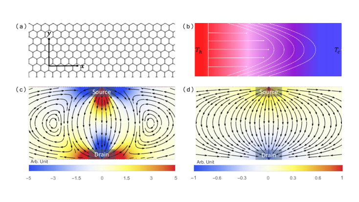
Figure 1: (a) A graphene nano-ribbon as a prototype 2D materials showing hydrodynamics phonon transport. (b) Schematic of Poiseuille flow generated by the temperature difference along the nano-ribbon. The heat flux has a parabolic distribution across the ribbon. (c) Heat current loops (lines) and temperature distribution (color) due to the viscosity of the phonon gas as signature of hydrodynamic heat transport. We set $\epsilon=1$. (d) The same as (c), but in the diffusive Fourier transport regime with $\epsilon=300$.

II The 2D G-K equation

We consider a prototype 2D material. It has one out-of-plane acoustic mode with a quadratic dispersion $\omega_{k}=ak^{2}$ (ZA mode), and two degenerate linear acoustic modes $\omega_{k}=v_{g}k$ (longitudinal and transverse). The magnitude of the linear group velocity is $v_{g}$, and the magnitude of the wave vector is $k=|\vec{k}|$. Here, in the spirit of Debye model, we ignore the possible anisotropic property and the difference between longitudinal and transverse branches. We will focus on the effect of ZA mode’s quadratic dispersion on the hydrodynamic behavior.

We first sketch the derivation of the 2D G-K equationGuyer and Krumhansl (1966a, b). Our starting point is the Peierls-Boltzmann equation under Callaway approximationCallaway (1959); Allen (2013)

$$\frac{\partial{f_{s\vec{k}}}}{\partial{t}}+\vec{v}_{s\vec{k}}\cdot\nabla{f}_{s\vec{k}}=-\frac{f_{s\vec{k}}-f_{R,s\vec{k}}^{eq}}{\tau_{R}}-\frac{f_{s\vec{k}}-f_{N,s\vec{k}}^{eq}}{\tau_{N}}.$$ (1)

Here, $s$ is the phonon index, $\tau_{N}$ is the constant relaxation time for the N-process, while $\tau_{R}$ is that for the resistive scattering process (R-process). It includes all scattering mechanisms that do not conserve crystal momentum, i. e., impurity scattering, phonon-scattering and other U-processes. We take the same $\tau_{R}$ and $\tau_{N}$ for all phonon branches, i.e., taking the wave vector and branch averaged values. This is the so-called gray approximation.

The N-process drives the system towards a displaced distribution function

$$f_{N,s\vec{k}}^{eq}=\left[e^{\beta_{B}(\hbar\omega_{s\vec{k}}-\hbar\vec{k}\cdot\vec{u})}-1\right]^{-1},$$ (2)

with $\beta_{B}=(k_{B}T)^{-1}$, and $\vec{u}$ is the drift velocity. But the R-process drives the system to an equilibrium Bose-Einstein distribution

$$f_{R,s\vec{k}}^{eq}=\left(e^{\beta_{B}\hbar\omega_{s\vec{k}}}-1\right)^{-1}.$$ (3)

It has been shown numerically that, within some moderate temperature range ($\sim 100$ K for graphene), the N-process is orders of magnitude faster than the R-process, meaning $\tau_{R}\gg\tau_{N}$Lee et al. (2015); Cepellotti et al. (2015). When the system size is much larger than the normal-scattering mean free path $l\approx v_{g}\tau_{N}$. The relaxation from local to global equilibrium or steady state is governed by hydrodynamic equations describing the conserved quantities during the $N$-process, including energy and crystal momentum.

As we know, conservation laws play central roles in the derivation of hydrodynamic equations. We consider energy and crystal momentum conservation here. Both normal (N) and resistive (R) scattering processes conserve total energy, giving

$$\sum_{s}\int\frac{d\vec{k}}{(2\pi)^{2}}\hbar\omega_{s\vec{k}}f_{s\vec{k}} =\sum_{s}\int\frac{d\vec{k}}{(2\pi)^{2}}\hbar\omega_{s\vec{k}}f_{N,s\vec{k}}^{eq},$$ (4)

$$\sum_{s}\int\frac{d\vec{k}}{(2\pi)^{2}}\hbar\omega_{s\vec{k}}f_{s\vec{k}} =\sum_{s}\int\frac{d\vec{k}}{(2\pi)^{2}}\hbar\omega_{s\vec{k}}f_{R,s\vec{k}}^{eq},$$ (5)

while only the N-process obeys crystal momentum conservation, giving

$$\sum_{s}\int\frac{d\vec{k}}{(2\pi)^{2}}\hbar\vec{k}f_{s\vec{k}}=\sum_{s}\int\frac{d\vec{k}}{(2\pi)^{2}}\hbar\vec{k}f_{N,s\vec{k}}^{eq}.$$ (6)

To get the equation governing the dynamics of the conserved quantity, we multiply by $\hbar\omega_{s\vec{k}}$, integrate over $\vec{k}$ and sum over the phonon index on both sides of Eq. (1). We then arrive at an equation describing energy conservation

$$\frac{\partial{E}}{\partial{t}}+\nabla\cdot\vec{q}=0,$$ (7)

where

$$E=\sum_{s}\int\frac{d\vec{k}}{(2\pi)^{2}}\hbar\omega_{s\vec{k}}f_{s\vec{k}}$$ (8)

is the total energy density, and

$$\vec{q}=\sum_{s}\int\frac{d\vec{k}}{(2\pi)^{2}}\hbar\omega_{s\vec{k}}\vec{v}_{s\vec{k}}f_{s\vec{k}}$$ (9)

is the heat current density. The right hand side of Eq. (7) is zero because the scattering processes conserve energy.

In principle, we can write down similar equation for the crystal momentum density $\vec{p}$ and its flux from its conservation law during $N$-processes. The G-K equation can be derived from the resulting momentum balance equation. This works well for the Debye model with linear phonon dispersion. But for graphene-like 2D system, the presence of quadratic dispersion leads to a divergent momentum flux, making further derivation difficultCepellotti (2016). To avoid this, we consider the heat flux directly, i.e., multiplying $\hbar\omega\vec{v}$ to each term in Eq. (1) and summing over all wave vectors and phonon indices. This leads to

$$\frac{\partial{\vec{q}}}{\partial{t}}+\frac{\vec{\kappa}}{\tau_{R}}\cdot\nabla T=-\frac{\vec{q}}{\tau_{R}}-\frac{\vec{q}_{1}}{\tau_{N}}.$$ (10)

Here, $\vec{q}_{1}$ is the 1st order term of heat flux, which will be explained below. We have also defined a thermal conductivity tensor as

$$\vec{\kappa}=\tau_{R}\sum_{s}\int\frac{d\vec{k}}{(2\pi)^{2}}\hbar\omega_{s\vec{k}}\vec{v}_{s\vec{k}}\vec{v}_{s\vec{k}}\frac{\partial f_{s\vec{k}}}{\partial T}.$$ (11)

To obtain the hydrodynamic equation, we rely on a multi-scale expansion technique developed recentlyGuo and Wang (2015). The expansion is over both space and time as follows:

$$\frac{\partial{}}{\partial{t}}= \varepsilon\frac{\partial}{\partial{t_{1}}}+\varepsilon^{2}\frac{\partial}{\partial{t_{2}}},$$ (12)

$$\frac{\partial{}}{\partial{x_{i}}}= \varepsilon\frac{\partial}{\partial{x_{1i}}}.$$ (13)

It is a perturbation expansion over a natural small parameter

$$\varepsilon=\frac{\tau_{N}}{\tau_{R}}.$$ (14)

That is to say, we consider the situation where the scattering rates of N-process is much larger than that of R-process. We expand the phonon distribution function as follows

$$f=f_{0}+\varepsilon f_{1}+\varepsilon^{2}f_{2}+\cdots,$$ (15)

with $f_{0}$, $f_{1}$, $f_{2}$ the 0th, 1st and 2nd order terms of phonon distribution function. The macroscopic variables can be expressed by the sum of approximate components

$$E=E_{0}+\varepsilon E_{1}+\varepsilon^{2}E_{2}+\cdots,$$

$$E_{n}=\sum_{s}\int\hbar\omega_{s\vec{k}}f_{n,s\vec{k}}\frac{d\vec{k}}{(2\pi)^{2}}.$$

$$\vec{q}=\vec{q}_{0}+\varepsilon\vec{q}_{1}+\varepsilon^{2}\vec{q}_{2}+\cdots,$$

$$\vec{q}_{n}=\sum_{s}\int\vec{v}_{s\vec{k}}\hbar\omega_{s\vec{k}}f_{n,s\vec{k}}\frac{d\vec{k}}{(2\pi)^{2}}.$$

$$\vec{\kappa}=\vec{\kappa}_{0}+\varepsilon\vec{\kappa}_{1}+\varepsilon^{2}\vec{\kappa}_{2}+\cdots,$$

$$\vec{\kappa}_{n}=\tau_{R}\sum_{s}\int\hbar\omega_{s\vec{k}}\vec{v}_{s\vec{k}}\vec{v}_{s\vec{k}}\frac{\partial f_{n,s\vec{k}}}{\partial T}\frac{d\vec{k}}{(2\pi)^{2}}.$$

We include the 0th and 1st order terms with $\vec{q}\approx\vec{q}_{0}+\varepsilon\vec{q}_{1}$, $\vec{\kappa}\approx\vec{\kappa}_{0}+\varepsilon\vec{\kappa}_{1}$. According to energy conservation (Eq. (4)), we know that $E=E_{0}$, since $E_{n}=0$ for $n>0$. All these are calculated from the distribution function $f\approx f_{0}+\varepsilon f_{1}$, with $f_{0}=f_{N}^{eq}$, $f_{1}=f_{R}^{eq}-f_{N}^{eq}-\tau_{N}\left(\partial_{t_{1}}f_{N}^{eq}+v_{i}\partial_{x_{1i}}{f_{N}^{eq}}\right)$. When $\vec{u}$ is small, we can approximate $f_{N}^{eq}$ as

$$f_{N}^{eq}\approx f_{R}^{eq}+\hbar\beta_{B}f_{R}^{eq}(f_{R}^{eq}+1)\vec{k}\cdot\vec{u}.$$ (16)

Numerical calculation shows that this is indeed a good approximationLee et al. (2015). Taking into account only the 0th order term $f_{0}$, we can get

$$E =\frac{2}{\pi}\frac{(k_{B}T)^{3}}{(\hbar v_{g})^{2}}Zeta(3)+\frac{\pi}{24}\frac{(k_{B}T)^{2}}{\hbar a}\equiv E_{L}+E_{N},$$ (17)

$$\vec{q}_{0} =\frac{3}{\pi}\frac{(k_{B}T)^{3}}{(\hbar v_{g})^{2}}Zeta(3)\vec{u}+\frac{\pi}{12}\frac{(k_{B}T)^{2}}{\hbar a}\vec{u}\equiv\vec{q}_{0L}+\vec{q}_{0N},$$ (18)

$$\vec{\kappa}_{0} =\frac{6Zeta(3)}{\pi}\frac{k_{B}^{3}T^{2}}{\hbar^{2}}\tau_{R}\vec{I}=C_{L}v_{g}^{2}\tau_{R}\vec{I}.$$ (19)

Here,$E_{L}$, $E_{N}$ are the equilibrium energy density of the linear and quadratic phonon modes, respectively. $\vec{q}_{0L}$, $\vec{q}_{0N}$ are the 0th order contribution of the linear and quadratic modes to the heat flux. They are both proportional to the drift velocity $\vec{u}$. $C_{L}=\left(\partial E_{L}/\partial T\right)=\frac{6Zeta(3)}{\pi}\frac{k_{B}^{3}}{(\hbar v_{g})^{2}}T^{2}$ is the specific heat capacity of the linear modes, $C_{N}$ is defined similarly, and $C=C_{L}+C_{N}$.

The first-order result of macroscopic variables are

$$E_{1} =0,$$ (20)

$$\vec{q}_{1} =0,$$ (21)

$$\vec{\kappa}_{1} =\tau_{R}\frac{\partial\vec{Q}}{\partial T}=\tau_{R}\left(\nabla\cdot\vec{Q}\right)\frac{1}{\nabla T}.$$ (22)

The expression of $\vec{Q}$ and calculation details can be found in the Appendix. We arrive at the G-K equation of 2D materials

$$\frac{\partial{\vec{q}}}{\partial{t}}+\frac{\kappa_{0}}{\tau_{R}}\nabla T+\frac{1}{\tau_{R}}\vec{q}=\eta\big{[}\nabla^{2}\vec{q}+2\nabla(\nabla\cdot\vec{q})\big{]}-\zeta\nabla(\nabla\cdot\vec{q}).$$ (23)

We have defined the 0th order thermal conductivity as $\kappa_{0}=\alpha C_{L}v_{g}^{2}\tau_{R}$, the first and second viscosity coefficients as $\eta=\beta v_{g}^{2}\tau_{N}$, $\zeta=\gamma v_{g}^{2}\tau_{N}$, with $\alpha=1$, $\beta=\frac{9E_{L}}{4(3E_{L}+4E_{N})}$, $\gamma=C_{L}/C$, respectively. Equation (23) with the above defined coefficients is the central results of this work. We can see that, although the form of the G-K equation is the same as the 3D case, the inclusion of quadratic phonon mode changes its coefficients. Notably, $\eta$ and $\gamma$ become temperature dependent, while for Debye model with three degenerate linear acoustic phonons modes, the coefficients are constant, with $\alpha=1/3$, $\beta=1/5$, $\gamma=1/3$ for 3D and $\alpha=1/2$, $\beta=1/4$, $\gamma=1/2$ for 2D case, respectively. In the following, we will analyze the consequences of this equation.

III Second sound and Poiseuille flow

We now analyze the consequence of Eq. (23). In this section, we show that, the numerical results in previous studiesLee et al. (2015); Cepellotti et al. (2015) can be obtained from Eq. (23) as special cases.

III.1 Second sound

The right side (RHS) of the G-K equation represents the effect of viscosity on the heat transport behavior. They come from the first order term in the expansion over $\varepsilon$. Before looking into these terms, we show here that the propagation of second sound can be analyzed without these terms. Replacing the RHS with zero, combining with Eq. (7), we arrive at

$$\frac{\partial^{2}T}{\partial t^{2}}+\frac{1}{\tau_{R}}\frac{\partial T}{\partial t}-v^{2}_{ss}\nabla^{2}T=0,$$ (24)

where we have defined the second sound velocity

$$v^{2}_{ss}=\frac{\kappa_{0}}{C\tau_{R}}=\alpha\gamma v_{g}^{2}.$$ (25)

This is the wave equation describing propagation of second sound with velocity $v_{ss}$ and damping coefficient $\tau_{R}^{-1}$. For 3D materials with the Debye model, the second sound velocity $v_{ss}=v_{g}/\sqrt{3}$, similar model for 2D material gives $v_{ss}=v_{g}/\sqrt{2}$. Here, the presence of quadratic dispersion makes $v_{ss}$ temperature dependent, inherited from the different temperature dependence of $C_{L}$ and $C_{N}$.

III.2 Poiseuille flow

We now include the RHS of the G-K equation, and consider a nano-ribbon with length $L$ ($0\leq x\leq L$) and width $w$ ($0\leq y\leq w$) [Fig. 1 (a)]. A temperature difference is applied along the ribbon ($x$ direction) [Fig. 1 (b)]. At steady state, ignoring $\vec{q}/\tau_{R}$, Eq. (23) reduces to a one-dimension form $\frac{\partial^{2}q}{\partial y^{2}}=A$. This gives rise to a parabolic heat flux distribution perpendicular to the flow $q(y)=\frac{A}{2}y(y-w)$, with $A=(\partial T/\partial x)\kappa_{0}/\tau_{R}\eta$, if we assume a non-slip boundary condition $q(0)=q(w)=0$. By integration over $y$, the heat current is obtained

$$I=\int_{0}^{w}q(y)dy=-\frac{1}{12}Aw^{3}.$$ (26)

The negative sign means heat flows opposite to the temperature gradient. The heat current scaling as $w^{3}$ is a signature of the Poiseuille flow. For diffusive phonon transport, the heat current scales linearly with the ribbon width $I\propto w$, while for ballistic transport, the heat current can not go higher than linear scaling with the width. Thus, the cubic (super-linear) dependence of $I$ on $w$ can in principle be used as a signature of the Poiseuille flow. The Poiseuille flow in graphene ribbons has been studied numerically by solving the Boltzmann equation directly in Refs. Lee et al., 2015; Cepellotti et al., 2015. Similar behavior is also predicted for electronic transport in graphene nano-ribbonsLevitov and Falkovich (2016). Length and width dependent thermal conductivity in suspended single layer graphene has been reported experimentallyBae et al. (2013); Xu et al. (2014). Thus, experimental confirmation of Poiseuille flow in graphene is already within reach.

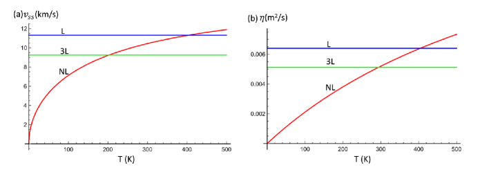
Figure 2: (a) The second sound velocity $v_{ss}$ as a function of temperature (T) for three different situations. (b) The dependence of the first viscosity coefficient $\eta$ on temperature (T). Here, we take the $\tau_{N}=10^{-10}$ s. NL stands for the 2D material with one quadratic ZA mode and two degenerate linear acoustic modes (longitudinal and transverse). L represents the 2D material with three degenerate linear acoustic phonons modes (2D Debye model). 3L means 3D material with three linear degenerate acoustic phonon modes (3D Debye model).

IV Heat current vortices and negative nonlocal conductance

One important consequence of Eq. (23) is nonlocal heat transport and formation of heat current vortices when there is a heat current source injecting into the 2D materials. As far as we know, this has not been considered before. To show this, we consider steady state transport in a setup sketched in Fig. 1 (c). Heat current source and drain are attached to a graphene nano-ribbon. The pattern of current flow at steady state can be obtained from the solution of simplified version of Eq. (23). At steady state, according to Eq. (7), we have $\partial\vec{q}/\partial t=\partial E/\partial t=0$. The resulting equation has the form

$$\eta\nabla^{2}\vec{q}-\tau_{R}^{-1}\vec{q}=C_{L}v_{g}^{2}\nabla T.$$ (27)

It shares the same form as the electronic case in Ref. Levitov and Falkovich, 2016. The 1st term on the left hand side (LHS) is the hydrodynamic term due to viscosity. It is the origin of the nonlocal transport behavior. When $\tau_{R}^{-1}$ is negligible, we get pure hydrodynamic viscous flow. One the other hand, when $\eta$ is negligible, we recover the normal diffusive heat transport governed by Fourier law. Thus, equation 27 applies to steady state diffusive and hydrodynamic transport. Actually, it is suggestive to define a dimensionless parameter

$$\epsilon=\frac{w^{2}}{\eta\tau_{R}}=\frac{w^{2}}{\beta v_{g}^{2}\tau_{N}\tau_{R}}$$ (28)

to characterize the relative contribution of diffusive and hydrodynamic transport.

As an example, we have plotted typical heat current flow patterns (lines) and the resulting temperature distribution (color) with $\epsilon=1$ and $300$ in Fig. 1 (c) and (d), respectively. Here, a flow of heat current from a point source $I(x)=I\delta(x)$ is injected into the ribbon and collected at the opposite side. The non-slip boundary condition is used to solve Eq. (27). The heat current flow within the ribbon can be obtained by solving Eq. (27) with the help of the streaming function. In Fig. 1 (c), hydrodynamic transport is dominant. The formation of vortices besides both sides of the direct source-to-drain flow is a characteristic feature of the viscous flow. Another prominent feature is the ‘separation’ of temperature gradient and heat flow. Even negative thermal resistance can be observed, where the heat current flows from the low to the high temperature regime. In Fig. 1 (d), the diffusive Fourier transport becomes dominant. Heat current vortices and negative resistance are absent. Thus, we can study the transition from hydrodynamic to Fourier transport by changing the magnitude of $\epsilon$.

We now give an order-of-magnitude analysis using parameters of graphene. We obtain the phonon dispersion relation of graphene using density function theory based calculations . Fitting the dispersion relation results in $v_{g}=1.6\times 10^{4}$ m/s for the linear modes, $a=5.5\times 10^{-7}$ m²/s for the quadratic mode. The specific heat capacity of them is given by $C_{L}=\frac{6Zeta(3)}{\pi}\frac{k_{B}^{3}T^{2}}{(\hbar v_{g})^{2}}\approx 2.14\times 10^{-9}T^{2}$ Jm^-2K^-1 and $C_{N}=\frac{\pi}{12}\frac{k_{B}^{2}T}{\hbar a}\approx 8.63\times 10^{-7}T$ Jm^-2K^-1, respectively. To estimate the transport coefficients and the dimensionless factor $\epsilon$, we use $\tau_{N}=10^{-10}$ s, $\tau_{R}=10^{-7}$ s Lee et al. (2015). We get $\beta\approx 0.08$ at $T=100$ K, smaller than value obtained from the 2D Debye model $\beta=1/4$. The different temperature dependence of $C_{L}$, $C_{N}$ and $E_{L}$, $E_{N}$ gives rise to temperature dependent $v_{ss}$ and $\eta$. This is contrast to 2D or 3D Debye model. The comparison of different situations is shown in Fig. 2 (a) and (b) for $v_{ss}$ and $\eta$, respectively. We find that, the presence of quadratic ZA mode reduces $v_{ss}$ and $\eta$ in the relevant temperature $\sim 100$ K. Still, we get $\eta\approx 0.002$ m²/s at $T=100$ K, which is orders of magnitude larger than that of water. We also get the dimensionless parameter $\epsilon\approx 5\times 10^{9}w^{2}$ m^-2. Thus, phonon hydrodynamic transport can be realized in high quality graphene nano-ribbons of micrometer scale. The plot in Fig. 1 (c) with $\epsilon=1$ corresponds to sample length of $\sim 15$ $\mu$m.

V Conclusions

In summary, we have derived a 2D version of the G-K equation describing hydrodynamic phonon heat transport. We take into account the out of plane quadratic phonon dispersion of the ZA mode, normally present in 2D materials. Its effect on the hydrodynamic transport is analyzed. The derived equation serves as a starting point for investigating nonlocal hydrodynamic phonon transport behavior in 2D materials. It shares similar form as the Navier-Stokes equation that has been used to study electron hydrodynamic transport in graphene. Many interesting transport behaviors, including nonlocal negative resistance, higher-than-ballistic transport, predicted for electrons can be studied for phonons. Moreover, a large overlap of the parameter regime between electron and phonon hydrodynamic transport in graphene makes it promising to study the effect of their mutual interaction on the thermal transport behavior of the two kinds of fluids.

During the submission of present work, several new studies came outZhang et al. (2019); Guo and Wang (2018); Li and Lee (2018), which are all based on numerical calculations and complementary to present analytical study.

Appendix A Derivation of the 2D G-K equation

Here, we give the derivation of Eq. (23) in the main text. We use the recent developed multiscale expansion techniqueGuo and Wang (2015). The expansion is over both space and time as follows:

$$\frac{\partial{}}{\partial{t}}= \varepsilon\frac{\partial}{\partial{t_{1}}}+\varepsilon^{2}\frac{\partial}{\partial{t_{2}}},$$ (29)

$$\frac{\partial{}}{\partial{x_{i}}}= \varepsilon\frac{\partial}{\partial{x_{1i}}},$$ (30)

where $\varepsilon$ is a small parameter, defined as

$$\varepsilon=\frac{\tau_{N}}{\tau_{R}}.$$ (31)

That is to say, we consider the situation where the scattering rates of N-process is much larger than that of R-process, preferential for hydrodynamic phonon transport. We expand the phonon distribution function as follows

$$f=f_{0}+\varepsilon f_{1}+\varepsilon^{2}f_{2}+\cdots,$$ (32)

with $f_{0}$, $f_{1}$, $f_{2}$ the 0th, 1st and 2nd order terms of phonon distribution function. The macroscopic variables can be expressed by the sum of approximate components

$$E =E_{0}+\varepsilon E_{1}+\varepsilon^{2}E_{2}+\cdots,\quad E_{n}=\sum_{s}\int\hbar\omega_{s\vec{k}}f_{n,s\vec{k}}\frac{d\vec{k}}{(2\pi)^{2}},$$ (33)

$$\vec{q} =\vec{q}_{0}+\varepsilon\vec{q}_{1}+\varepsilon^{2}\vec{q}_{2}+\cdots,\quad\vec{q}_{n}=\sum_{s}\int\vec{v}_{s\vec{k}}\hbar\omega_{s\vec{k}}f_{n,s\vec{k}}\frac{d\vec{k}}{(2\pi)^{2}},$$ (34)

$$\vec{\kappa} =\vec{\kappa}_{0}+\varepsilon\vec{\kappa}_{1}+\varepsilon^{2}\vec{\kappa}_{2}+\cdots,\quad\vec{\kappa}_{n}=\tau_{R}\sum_{s}\int\hbar\omega_{s\vec{k}}\vec{v}_{s\vec{k}}\vec{v}_{s\vec{k}}\frac{\partial f_{n,s\vec{k}}}{\partial T}\frac{d\vec{k}}{(2\pi)^{2}}.$$ (35)

Substituting all of the equations above into the Peierls-Boltzmann equation, we obtain the 0th and 1st order terms of phonon distribution function:

$$f_{0} =f_{N}^{eq},$$ (36)

$$f_{1} =f_{R}^{eq}-f_{N}^{eq}-\tau_{N}\left(\frac{\partial{f_{N}^{eq}}}{\partial t_{1}}+v_{i}\frac{\partial{f_{N}^{eq}}}{\partial x_{1i}}\right),$$ (37)

and different order of approximations for the balance equations

$$\frac{\partial{E}}{\partial{t_{1}}} +\frac{\partial{}}{\partial{x_{1i}}}q_{0i}=0,$$ (38)

$$\frac{\partial{E}}{\partial{t_{2}}} +\frac{\partial{}}{\partial{x_{1i}}}q_{1i}=0,$$ (39)

$$\frac{\partial{q_{0i}}}{\partial{t_{1}}} +\kappa_{0ij}\frac{\partial{T}}{\partial{x_{1j}}}=-\frac{1}{\tau_{N}}q_{0i}-\frac{1}{\tau_{N}}q_{1i},$$ (40)

$$\frac{\partial{q_{0i}}}{\partial{t_{2}}} +\frac{\partial{q_{1i}}}{\partial{t_{1}}}+\kappa_{1ij}\frac{\partial{T}}{\partial{x_{1j}}}=-\frac{1}{\tau_{N}}q_{1i}-\frac{1}{\tau_{N}}q_{2i}.$$ (41)

A.1 The zeroth-order result

We calculate the macroscopic variables including the energy density, the heat flux and the thermal conductivity, taking into account the 0th order term $f_{0}$. We make the following approximation

$$f_{0}=f_{N}^{eq}=f_{R}^{eq}+f_{N1}^{eq}\approx f_{R}^{eq}+\beta_{B}f_{R}^{eq}(f_{R}^{eq}+1)\hbar\vec{k}\cdot\vec{u},$$ (42)

whose validity has been checked numericallyLee et al. (2015).

A.1.1 Energy density

We consider the phonon energy density first. According to energy conservation (4), we know that $E=E_{0}$,

$$E=\sum_{s}\int\hbar\omega_{s\vec{k}}f_{N,s\vec{k}}^{eq}\frac{d\vec{k}}{(2\pi)^{2}}=\sum_{s}\int\hbar\omega_{s\vec{k}}f_{R,s\vec{k}}^{eq}\frac{d\vec{k}}{(2\pi)^{2}}+\sum_{s}\int\hbar\omega_{s\vec{k}}f_{R,s\vec{k}}^{eq}\left(1+f_{R,s\vec{k}}^{eq}\right)\frac{\hbar\vec{k}\cdot\vec{u}}{k_{B}T}\frac{d\vec{k}}{(2\pi)^{2}}.$$ (43)

The second term in the above equation vanishes because it’s an odd function of $\vec{k}$. Thus we arrive at:

$$E=\sum_{s}\int\hbar\omega_{s\vec{k}}f_{R,s\vec{k}}^{eq}\frac{d\vec{k}}{(2\pi)^{2}}=\frac{2}{\pi}\frac{(k_{B}T)^{3}}{(\hbar v_{g})^{2}}Zeta(3)+\frac{\pi}{24}\frac{(k_{B}T)^{2}}{\hbar a}\equiv E_{L}+E_{N}.$$ (44)

Here, $E_{L}$ and $E_{N}$ are the energy density of linear and quadratic phonon modes, respectively. Note that we have included the factor 2 to account the degeneracy of the linear phonon modes.

A.1.2 Heat flux

The 0th order heat flux is calculated as

$$\vec{q}_{0}=\sum_{s}\int\vec{v}_{s\vec{k}}\hbar\omega_{s\vec{k}}f_{N,s\vec{k}}^{eq}\frac{d\vec{k}}{(2\pi)^{2}}=\sum_{s}\int\vec{v}_{s\vec{k}}\hbar\omega_{s\vec{k}}f_{R,s\vec{k}}^{eq}\frac{d\vec{k}}{(2\pi)^{2}}+\sum_{s}\int\vec{v}_{s\vec{k}}\hbar\omega_{s\vec{k}}f_{N1,s\vec{k}}^{eq}\frac{d\vec{k}}{(2\pi)^{2}}.$$ (45)

Since at thermal equilibrium, the heat flux is zero. Only the second term contributes

$$\vec{q}_{0}=\sum_{s}\int\vec{v}_{s\vec{k}}\hbar\omega_{s\vec{k}}f_{N1,s\vec{k}}^{eq}\frac{d\vec{k}}{(2\pi)^{2}}=\frac{3}{\pi}\frac{(k_{B}T)^{3}}{(\hbar v_{g})^{2}}Zeta(3)\vec{u}+\frac{\pi}{12}\frac{(k_{B}T)^{2}}{\hbar a}\vec{u}\equiv\vec{q}_{0L}+\vec{q}_{0N}.$$ (46)

Here, $\vec{q}_{0L}$, $\vec{q}_{0N}$ are the 0th order contribution of the linear and quadratic modes to the heat flux.

A.1.3 Thermal conductivity tensor

The thermal conductivity tensor is

$$\vec{\kappa}_{0} =\tau_{R}\sum_{s}\int\hbar\omega_{s\vec{k}}\vec{v}_{s\vec{k}}\vec{v}_{s\vec{k}}\frac{\partial f_{N,s\vec{k}}^{eq}}{\partial T}\frac{d\vec{k}}{(2\pi)^{2}}=\tau_{R}\sum_{s}\int\hbar\omega_{s\vec{k}}\vec{v}_{s\vec{k}}\vec{v}_{s\vec{k}}\frac{\partial f_{R,s\vec{k}}^{eq}}{\partial T}\frac{d\vec{k}}{(2\pi)^{2}}+\tau_{R}\sum_{s}\int\hbar\omega_{s\vec{k}}\vec{v}_{s\vec{k}}\vec{v}_{s\vec{k}}\frac{\partial f_{N1,s\vec{k}}^{eq}}{\partial T}\frac{d\vec{k}}{(2\pi)^{2}}.$$ (47)

Likewise, the second term in the above equation is an odd function of $\vec{k}$ and thus is zero. We then have

$$\vec{\kappa}_{0} =\tau_{R}\sum_{s}\int\hbar\omega_{s\vec{k}}\vec{v}_{s\vec{k}}\vec{v}_{s\vec{k}}\frac{\partial f_{R,s\vec{k}}^{eq}}{\partial T}\frac{d\vec{k}}{(2\pi)^{2}}=\tau_{R}\sum_{s}\int\hbar\omega_{s\vec{k}}\vec{v}_{s\vec{k}}\vec{v}_{s\vec{k}}f_{R,s\vec{k}}^{eq}\left(f_{R,s\vec{k}}^{eq}+1\right)\frac{\hbar\omega_{s\vec{k}}}{k_{B}T^{2}}\frac{d\vec{k}}{(2\pi)^{2}}$$

$$=\frac{3}{\pi}\frac{k_{B}^{3}T^{2}}{\hbar^{2}}Zeta(3)\tau_{R}\vec{I}+\frac{3}{\pi}\frac{k_{B}^{3}T^{2}}{\hbar^{2}}Zeta(3)\tau_{R}\vec{I}\equiv\vec{\kappa}_{0L}+\vec{\kappa}_{0N}.$$ (48)

We get the 0th order thermal conductivity contributed from the linear $\vec{\kappa}_{0L}$ and quadratic modes $\vec{\kappa}_{0N}$. It is noted that, given a constant $\tau_{R}$, the thermal conductivity contributed from a quadratic mode is two times larger than that contributed from a linear mode. Both of them are independent of the details of the dispersion. So we can rewrite $\kappa_{0}$ in terms of the energy density of the linear phonon modes,

$$\vec{\kappa}_{0}=\frac{6Zeta(3)}{\pi}\frac{k_{B}^{3}T^{2}}{\hbar^{2}}\tau_{R}\vec{I}=C_{L}v_{g}^{2}\tau_{R}\vec{I},$$ (49)

where the specific heat capacity of the linear modes is:

$$C_{L}=\frac{\partial E_{L}}{\partial T}=\frac{6Zeta(3)}{\pi}\frac{k_{B}^{3}}{(\hbar v_{g})^{2}}T^{2}.$$

A.2 The first-order result

Now, we calculate the 1st order terms in the expansion

$$f_{1} =f_{R}^{eq}-f_{N}^{eq}-\tau_{N}\left(\frac{\partial{f_{N}^{eq}}}{\partial t_{1}}+v_{i}\frac{\partial{f_{N}^{eq}}}{\partial x_{1i}}\right).$$ (50)

Based on the chain rule

$$\frac{\partial{f_{N}^{eq}}}{\partial{t_{1}}} =\frac{\partial{f_{N}^{eq}}}{\partial{u_{j}}}\frac{\partial{u_{j}}}{\partial{t_{1}}}+\frac{\partial{f_{N}^{eq}}}{\partial{T}}\frac{\partial{T}}{\partial{t_{1}}},$$ (51)

$$\frac{\partial{f_{N}^{eq}}}{\partial{x_{1i}}} =\frac{\partial{f_{N}^{eq}}}{\partial{u_{j}}}\frac{\partial{u_{j}}}{\partial{x_{1i}}}+\frac{\partial{f_{N}^{eq}}}{\partial{T}}\frac{\partial{T}}{\partial{x_{1i}}},$$ (52)

and the approximation for $f_{N}^{eq}$, combined with Eqs. (38),(39), we arrive at a lengthy expression for $f_{1}$ :

$$f_{1}=-\frac{\hbar\vec{k}\vec{u}}{k_{B}T}f_{R}^{eq}\left(f_{R}^{eq}+1\right)-\tau_{N}f_{R}^{eq}\left(f_{R}^{eq}+1\right)\left\{\frac{\hbar k_{i}}{k_{B}T}\left(-\frac{2C_{L}v_{g}^{2}}{3E_{L}+4E_{N}}\frac{\partial T}{\partial x_{1i}}+\frac{u_{i}}{3E_{L}+4E_{N}}\frac{3C_{L}+4C_{N}}{C}\frac{\partial q_{0j}}{\partial x_{1j}}-\right.\right.\\ \left.\left.\frac{2}{3E_{L}+4E_{N}}\frac{q_{0i}}{\tau_{N}}\right)+\left(\frac{v}{k}k_{i}\frac{\partial T}{\partial{x_{1i}}}-\frac{1}{C}\frac{\partial q_{0j}}{\partial x_{1j}}\right)\left[\frac{\hbar\omega}{k_{B}T^{2}}+\frac{\hbar\omega}{k_{B}T^{2}}\left(2f_{R}^{eq}+1\right)\frac{\hbar\vec{k}\vec{u}}{k_{B}T}-\frac{\hbar\vec{k}\vec{u}}{k_{B}T^{2}}\right]+\frac{v}{k}\frac{\hbar k_{i}k_{j}}{k_{B}T}\frac{\partial}{\partial{x_{1i}}}\left(\frac{2q_{0j}}{3E_{L}+4E_{N}}\right)\right\}.$$ (53)

We notice from eqs. (38-41) that, $f_{1}$ depends on $\vec{q}_{1}$, while to obtain $\vec{q}_{1}$ we need $f_{1}$. In principle, we need to self-consistent calculations of them. Here, to arrive at analytical result, we made the truncation and set $\vec{q}_{1}=0$ in eqs. (38-41).

A.2.1 Phonon energy density

According to the foregoing discussion, we can get :

$$E =E_{0}.$$ (54)

The higher order terms of distribution function do not contribute to the energy density.

A.2.2 Heat flux

Using the truncation we made for $f_{1}$, we can check that $\vec{q}_{1}=0$ if we plug Eq. (53) into Eq. (34)

$$\vec{q}_{1} =\sum_{s}\int\hbar\omega_{s\vec{k}}\vec{v}_{s\vec{k}}f_{1,s\vec{k}}\frac{d\vec{k}}{(2\pi)^{2}}=\vec{q}_{1L}+\vec{q}_{1N}=0,$$ (55)

as required by our truncation scheme.

A.2.3 Thermal conductivity tensor

Finally, we consider the thermal conductivity tensor. We consider the linear and quadratic modes separately

$$\vec{\kappa}_{1} =\tau_{R}\frac{\partial}{\partial T}\left(\vec{Q}_{L}+\vec{Q}_{N}\right),$$ (56)

with $\vec{Q}_{L}$, $\vec{Q}_{N}$ corresponding to the contribution from linear and quadratic modes, respectively. Again, the odd parts do not contribute to the integral. Collecting the even parts, we divide $\vec{Q}_{L}$ into three parts:

$$\vec{Q}_{L}= \vec{Q}_{L,I}+\vec{Q}_{L,II}+\vec{Q}_{L,III},$$ (57)

with each part written as

$$(Q_{L,I})_{mn} =\frac{1}{2}\tau_{N}v_{g}^{2}\frac{C_{L}}{C}\frac{\partial q_{0j}}{\partial x_{1j}}\delta_{mn},$$ (58)

$$(Q_{L,II})_{mn} =-\frac{3}{4}v_{g}^{2}E_{L}\tau_{N}\left[\frac{\partial}{\partial x_{1i}}\left(\frac{q_{0i}}{3E_{L}+4E_{N}}\right)\delta_{mn}+\frac{\partial}{\partial x_{1m}}\left(\frac{q_{0n}}{3E_{L}+4E_{N}}\right)+\frac{\partial}{\partial x_{1n}}\left(\frac{q_{0m}}{3E_{L}+4E_{N}}\right)\right],$$ (59)

$$(Q_{L,III})_{mn} =-\frac{3}{4}\frac{v_{g}^{2}\tau_{N}}{T}\left[\left(q_{0L}\right)_{i}\frac{\partial T}{\partial x_{1i}}\delta_{mn}+\left(q_{0L}\right)_{n}\frac{\partial T}{\partial x_{1m}}+\left(q_{0L}\right)_{m}\frac{\partial T}{\partial x_{1n}}\right].$$ (60)

Similarly,

$$\vec{Q}_{N}= \vec{Q}_{N,I}+\vec{Q}_{N,II}+\vec{Q}_{N,III},$$ (61)

with

$$(Q_{N,I})_{mn} =\frac{1}{2}\tau_{N}v_{g}^{2}\frac{C_{L}}{C}\frac{\partial q_{0j}}{\partial x_{1j}}\delta_{mn},$$ (62)

$$(Q_{N,II})_{mn} =-\frac{3}{2}v_{g}^{2}E_{L}\tau_{N}\left[\frac{\partial}{\partial x_{1i}}\left(\frac{q_{0i}}{3E_{L}+4E_{N}}\right)\delta_{mn}+\frac{\partial}{\partial x_{1m}}\left(\frac{q_{0n}}{3E_{L}+4E_{N}}\right)+\frac{\partial}{\partial x_{1n}}\left(\frac{q_{0m}}{3E_{L}+4E_{N}}\right)\right],$$ (63)

$$(Q_{N,III})_{mn} =-\frac{3}{2}\frac{v_{g}^{2}\tau_{N}}{T}\left[\left(q_{0L}\right)_{i}\frac{\partial T}{\partial x_{1i}}\delta_{mn}+\left(q_{0L}\right)_{n}\frac{\partial T}{\partial x_{1m}}+\left(q_{0L}\right)_{m}\frac{\partial T}{\partial x_{1n}}\right].$$ (64)

Summing up the linear and nonlinear results gives

$$(Q_{I})_{mn} =\tau_{N}v_{g}^{2}\frac{C_{L}}{C}\frac{\partial q_{0j}}{\partial x_{1j}}\delta_{mn},$$ (65)

$$(Q_{II})_{mn} =-\frac{9}{4}v_{g}^{2}E_{L}\tau_{N}\left[\frac{\partial}{\partial x_{1i}}\left(\frac{q_{0i}}{3E_{L}+4E_{N}}\right)\delta_{mn}+\frac{\partial}{\partial x_{1m}}\left(\frac{q_{0n}}{3E_{L}+4E_{N}}\right)+\frac{\partial}{\partial x_{1n}}\left(\frac{q_{0m}}{3E_{L}+4E_{N}}\right)\right],$$ (66)

$$(Q_{III})_{mn} =-\frac{9}{4}\frac{v_{g}^{2}\tau_{N}}{T}\left[\left(q_{0L}\right)_{i}\frac{\partial T}{\partial x_{1i}}\delta_{mn}+\left(q_{0L}\right)_{n}\frac{\partial T}{\partial x_{1m}}+\left(q_{0L}\right)_{m}\frac{\partial T}{\partial x_{1n}}\right],$$ (67)

and $\kappa_{1}$ is obtained from

$$\vec{\kappa}_{1}=\tau_{R}\frac{\partial\vec{Q}}{\partial T}=\tau_{R}\left(\nabla\cdot\vec{Q}\right)\frac{1}{\nabla T}.$$ (68)

A.3 The G-K equation

Substituting the calculated 0th and 1st order results into Eq. (10), neglecting the nonlinear effects resulting from the product of heat flux and temperature gradient in $\kappa_{1}$, we get the G-K equation

$$\frac{\partial{\vec{q}}}{\partial{t}}+\frac{\kappa_{0}}{\tau_{R}}\nabla T+\frac{1}{\tau_{R}}\vec{q}=\eta\big{[}\nabla^{2}\vec{q}+2\nabla(\nabla\cdot\vec{q})\big{]}-\zeta\nabla(\nabla\cdot\vec{q}).$$ (69)

The transport coefficients are $\kappa_{0}=\alpha C_{L}v_{g}^{2}\tau_{R}$, $\eta=\beta v_{g}^{2}\tau_{N}$, $\xi=\gamma v_{g}^{2}\tau_{N}$, with $\alpha=1$, $\beta=\frac{9}{4}\frac{E_{L}}{3E_{L}+4E_{N}}$, $\gamma=\frac{C_{L}}{C}$, respectively. For comparison, we also consider the 2D Debye model with three degenerate acoustic phonon modes. The resulting equation is the same, but with the coefficients $\alpha=\frac{1}{2}$, $\beta=\frac{1}{4}$, $\gamma=\frac{1}{2}$. These results can be compared with the 3D Debye model, resulting in $\alpha=\frac{1}{3}$, $\beta=\frac{1}{5}$, $\gamma=\frac{1}{3}$.

References

- Gurzhi (1968) R. N. Gurzhi, Sov. Phys. Usp. 11, 255 (1968).
- Beck et al. (1974) H. Beck, P. F. Meier, and A. Thellung, Phys. Stat. Sol. (a) 24, 11 (1974).
- de Jong and Molenkamp (1995) M. J. M. de Jong and L. W. Molenkamp, Phys. Rev. B 51, 13389 (1995).
- Bandurin et al. (2016) D. A. Bandurin, I. Torre, R. K. Kumar, M. B. Shalom, A. Tomadin, A. Principi, G. H. Auton, E. Khestanova, K. S. Novoselov, I. V. Grigorieva, L. A. Ponomarenko, A. K. Geim, and M. Polini, Science 351, 1055 (2016).
- Crossno et al. (2016) J. Crossno, J. K. Shi, K. Wang, X. Liu, A. Harzheim, A. Lucas, S. Sachdev, P. Kim, T. Taniguchi, K. Watanabe, T. A. Ohki, and K. C. Fong, Science 351, 1058 (2016).
- Moll et al. (2016) P. J. W. Moll, P. Kushwaha, N. Nandi, B. Schmidt, and A. P. Mackenzie, Science 351, 1061 (2016).
- de Tomas et al. (2014) C. de Tomas, A. Cantarero, A. F. Lopeandia, and F. X. Alvarez, J. Appl. Phys. 115, 164314 (2014).
- Sellitto et al. (2015) A. Sellitto, I. Carlomagno, and D. Jou, Proc. R. Soc. A 471, 20150376 (2015).
- Guo and Wang (2015) Y. Guo and M. Wang, Phys. Rep. 595, 1 (2015).
- Cepellotti et al. (2015) A. Cepellotti, G. Fugallo, L. Paulatto, M. Lazzeri, F. Mauri, and N. Marzari, Nat. Commun. 6, 6400 (2015).
- Lee et al. (2015) S. Lee, D. Broido, K. Esfarjani, and G. Chen, Nat. Commun. 6, 6290 (2015).
- Levitov and Falkovich (2016) L. Levitov and G. Falkovich, Nat. Phys. 12, 672 (2016).
- Cao et al. (2011) C. Cao, E. Elliott, J. Joseph, H. Wu, J. Petricka, T. Schäfer, and J. E. Thomas, Science 331, 58 (2011).
- Jacak and Müller (2012) B. V. Jacak and B. Müller, Science 337, 310 (2012).
- Gu et al. (2018) X. Gu, Y. Wei, X. Yin, B. Li, and R. Yang, Rev. Mod. Phys. 90, 041002 (2018).
- Li et al. (2012) N. Li, J. Ren, L. Wang, G. Zhang, P. Hänggi, and B. Li, Rev. Mod. Phys. 84, 1045 (2012).
- Wang et al. (2008) J.-S. Wang, J. Wang, and J.-T. Lü, Eur. Phys. J. B 62, 381 (2008).
- Gooth et al. (2017) J. Gooth, F. Menges, C. Shekhar, V. Süß, N. Kumar, Y. Sun, U. Drechsler, R. Zierold, C. Felser, and B. Gotsmann, arXiv:1706.05925 (2017).
- Guo et al. (2017) H. Guo, E. Ilseven, G. Falkovich, and L. Levitov, PNAS 114, 3068 (2017).
- Falkovich and Levitov (2017) G. Falkovich and L. Levitov, Phys. Rev. Lett. 119, 066601 (2017).
- Alekseev (2016) P. Alekseev, Phys. Rev. Lett. 117, 166601 (2016).
- Pellegrino et al. (2016) F. M. D. Pellegrino, I. Torre, A. K. Geim, and M. Polini, Phys. Rev. B 94, 155414 (2016).
- Briskot et al. (2015) U. Briskot, M. Schütt, I. V. Gornyi, M. Titov, B. N. Narozhny, and A. D. Mirlin, Phys. Rev. B 92, 115426 (2015).
- Narozhny et al. (2015) B. N. Narozhny, I. V. Gornyi, M. Titov, M. Schütt, and A. D. Mirlin, Phys. Rev. B 91, 035414 (2015).
- Lucas and Fong (2018) A. Lucas and K. C. Fong, J. Phys.: Condens. Matter 30, 053001 (2018).
- Cepellotti and Marzari (2016) A. Cepellotti and N. Marzari, Phys. Rev. X 6, 041013 (2016).
- Cepellotti and Marzari (2017) A. Cepellotti and N. Marzari, Phys. Rev. Materials 1, 045406 (2017).
- Lee and Lindsay (2017) S. Lee and L. Lindsay, Phys. Rev. B 95, 184304 (2017).
- Ding et al. (2018) Z. Ding, J. Zhou, B. Song, V. Chiloyan, M. Li, T.-H. Liu, and G. Chen, Nano Lett. 18, 638 (2018).
- Guo and Wang (2017) Y. Guo and M. Wang, Phys. Rev. B 96, 134312 (2017).
- Ackerman et al. (1966) C. C. Ackerman, B. Bertman, H. A. Fairbank, and R. A. Guyer, Phys. Rev. Lett. 16, 789 (1966).
- Narayanamurti and Dynes (1972) V. Narayanamurti and R. C. Dynes, Phys. Rev. Lett. 28, 1461 (1972).
- Jackson et al. (1970) H. E. Jackson, C. T. Walker, and T. F. McNelly, Phys. Rev. Lett. 25, 26 (1970).
- Martelli et al. (2018) V. Martelli, J. L. Jiménez, M. Continentino, E. Baggio-Saitovitch, and K. Behnia, Phys. Rev. Lett. 120, 125901 (2018).
- Machida et al. (2018) Y. Machida, A. Subedi, K. Akiba, A. Miyake, M. Tokunaga, Y. Akahama, K. Izawa, and K. Behnia, Sci Adv 4, eaat3374 (2018).
- Markov et al. (2018) M. Markov, J. Sjakste, G. Barbarino, G. Fugallo, L. Paulatto, M. Lazzeri, F. Mauri, and N. Vast, Phys. Rev. Lett. 120, 075901 (2018).
- Guyer and Krumhansl (1966a) R. A. Guyer and J. A. Krumhansl, Phys. Rev. 148, 766 (1966a).
- Guyer and Krumhansl (1966b) R. A. Guyer and J. A. Krumhansl, Phys. Rev. 148, 778 (1966b).
- Callaway (1959) J. Callaway, Phys. Rev. 113, 1046 (1959).
- Allen (2013) P. B. Allen, Phys. Rev. B 88, 144302 (2013).
- Cepellotti (2016) A. Cepellotti, Thermal transport in low dimensions, Ph.D. thesis, EPFL (2016).
- Bae et al. (2013) M.-H. Bae, Z. Li, Z. Aksamija, P. N. Martin, F. Xiong, Z.-Y. Ong, I. Knezevic, and E. Pop, Nat. Commun. 4, 1734 (2013).
- Xu et al. (2014) X. Xu, L. F. C. Pereira, Y. Wang, J. Wu, K. Zhang, X. Zhao, S. Bae, C. Tinh Bui, R. Xie, J. T. L. Thong, B. H. Hong, K. P. Loh, D. Donadio, B. Li, and B. Özyilmaz, Nat. Commun. 5, 3689 (2014).
- Note (1) For the density functional theory calculation, we use the Vienna Ab-initio Simulation Package and the generalized gradient approximation for the exchange-correlation functional. The parameters are the same as Ref. \rev@citealpnumGe2016.
- Zhang et al. (2019) C. Zhang, Z. Guo, and S. Chen, International Journal of Heat and Mass Transfer 130, 1366 (2019).
- Guo and Wang (2018) Y. Guo and M. Wang, Phys. Rev. B 97, 035421 (2018).
- Li and Lee (2018) X. Li and S. Lee, Phys. Rev. B 97, 094309 (2018).
- Ge et al. (2016) X.-J. Ge, K.-L. Yao, and J.-T. Lü, Phys. Rev. B 94, 165433 (2016).