On the stability of persistent entropy and new summary functions for Topological Data Analysis
On the stability of persistent entropy and new summary functions for Topological Data Analysis
Abstract
Persistent homology and persistent entropy have recently become useful tools for patter recognition. In this paper, we find requirements under which persistent entropy is stable to small perturbations in the input data and scale invariant. In addition, we describe two new stable summary functions combining persistent entropy and the Betti curve. Finally, we use the previously defined summary functions in a material classification task to show their usefulness in machine learning and pattern recognition.
Department of Applied Mathematics I, University of Seville
{natienza, rogodi, msoriano4}@us.es
1 Introduction
Topological data analysis (TDA) uses computational topology tools to study datasets. Intuitively, topological features like homology can be seen as qualitative geometric properties related to the notions of proximity and continuity and, therefore, can be useful tools for pattern recognition [1]. TDA has become a large field of research, with persistent homology (and its precursor known as size functions [2]) as its key tool. It has been applied successfully in many areas (see, for example, [3]). Its standard workflow is the following (see also Figure 1):
-
1.
Start with a dataset, for example, a point cloud, endowed with some notion of proximity (usually a metric).
-
2.
Depending on the kind of information we want to obtain, build a simplicial complex and a filter function on it. Compute a nested sequence of increasing subcomplexes (which encapsulate features from data) using the filter function.
-
3.
Compute the homology of each subcomplex (intuitively, homology captures the “holes” of the underlying space) and study how it evolves in the sequence, leading to the key concept of persistent homology.
Persistent homology can be compactly represented using persistence barcodes [4], diagrams [5] and, more recently, landscapes [6]. There exist stability results showing that these representations are robust under small perturbations of the given data (see, for example, [7]). In addition, there are numerous software packages to calculate persistent homology and its representations. A nice study of the performance of available software packages is made in [8].
Although persistence barcodes, diagrams, and landscapes are metric spaces
used to compare persistent homology of datasets, persistence barcodes and diagrams do not work properly for statistical analysis. For example, they fail to have unique mean (see [9]). Persistence landscapes perform better [6], but they are limited to the context of probability in Banach spaces.
It is more useful sometimes to summarize the information contained in persistent homology using only a number.
It becomes especially appropriate when only small samples are available since univariate non-parametric tests are required in these cases.
Persistent entropy seems to be a perfect candidate to summarize persistent homology using only a number. Specifically, persistent entropy is the Shannon entropy [10] of a probability distribution obtained from persistent homology.
It was defined in its current form in [11] but a precursor of this definition appears in [12]. Some successful applications of persistent entropy have been developed for pattern recognition of signals [13, 14], complex systems [15], biological images [16] and clustering [17]. A more theoretical approach allows persistent entropy to be used to distinguish topological features from noise [18].
With regards to implementation, persistent entropy has already been implemented as a method in Gudhi library111
https://github.com/GUDHI/gudhi-devel/blob/master/src/python/gudhi/
representations/vector_methods.py , scikit-TDA library222https://github.com/scikit-tda/persim and
Giotto library333https://github.com/giotto-ai/giotto-learn/blob/master/giotto/diagrams/features.py.
Some partial results about stability of persistent entropy have been given in [14, 18] but, as far as we know, no formal study of persistent entropy has been done.
The main objective of this paper is to provide a general stability result for persistent entropy and to study under which conditions persistent entropy is scale-invariant.
When it is not necessary to find significant differences in data but a classification task is needed, the usual approach is to replace statistical tests with machine learning methods. In this case, summarizing persistent homology in a number may be too restrictive, since we are projecting an infinite-dimensional space (persistence barcodes) to only one dimension (persistent entropy). One solution might be to use summary functions instead. Common approaches to summarizing persistence barcodes include kernel functions such as persistence multi-scale kernel [19], persistence weighted Gaussian kernel [20] and sliced Wasserstein kernel [21], as well as persistence-diagram vectorizations such as the already mentioned persistence landscape, persistence silhouettes [22], persistence images [23], Euler characteristic curves [24], topological intensity maps [25] and Betti curves [26, 27]. In this paper, we will define two new stable summary functions based on persistent entropy that can be used as a complementary function to the previous ones to describe persistence barcodes.
The paper is organized as follows. After recalling the theory of persistent homology in Section 2, stability and scale-invariance of persistent entropy is introduced in Section 3. In Section 4, we define two new summary functions derived from the concept of persistent entropy and study also their stability. Examples showing the applicability of these functions are also given. The usefulness of the summary functions defined in this paper is showed in Section 5. The paper ends with a section devoted to conclusions and future work.
2 Background
In this section, we give a quick overview of how algebraic topology is applied to data analysis. An instructive book showing the main algebraic topology tools for data analysis is [7].
As explained in the introduction, in order to apply algebraic topology tools to data analysis, we first must summarize the information provided by the data in a combinatorial structure, the simplicial complex structure being the most commonly used. Recall that an -simplex is the convex hull of affinely independent points. A -simplex is a point, a -simplex is a segment, a -simplex is a triangle, a -simplex is a tetrahedron and so on. A simplicial complex is a set of simplices glued in a specific way. An abstract simplicial complex can be seen as a way of storing the combinatorial structure of a simplicial complex.
Definition 2.1 (abstract simplicial complex).
Let be a finite set. A family of subsets of is an abstract simplicial complex if for every subsets and , we have that implies (in other words, non-empty intersections of simplices in are also simplices of ). A subset in of elements of is called an -simplex.
When the finite set represents data, the geometrical structure of its associated simplicial complex can provide information about how the data is related. Usually, these relations are not equally significant so it is common to define an order in its simplices to represent their importance. This can be done implicitly using a filter function.
Definition 2.2 (filtration).
A filter function on a simplicial complex is a monotonic function satisfying that implies . A filtration on , obtained from , is the sequence of subcomplexes where .
Notice that, because of the monotonicity of , the set is a simplicial complex for all , and implies that . To help intuition, the parameter will be referred as time although its physical meaning may be completely different. The following definition is an example of filtration and requires to be a metric space.
Definition 2.3 (Vietoris-Rips filtration).
Let be a finite set of points endowed with a distance . The Vietoris-Rips filtration of is the sequence obtained from the filter function
where, for each , the simplices of the Vietoris-Rips simplicial complex are defined as:
Homology groups of simplicial complexes provide a formal interpretation of what an -dimensional “hole” is. Intuitively, a -dimensional hole is a connected component, a -dimensional hole is a loop, a -dimensional hole is a cavity, and so on. Given a simplicial complex , an -chain is a formal sum of -simplices of . That is, where, for , is an -simplex of and is a coefficient in an unital ring . To relate the -chains of a given simplicial complex with its -dimensional holes, we need the boundary operator : If is an -simplex of then,
We can extend this definition to any -chain by linearity. Notice that or, in other words, the boundary of a boundary is null. The -dimensional holes of are detected from -chains whose boundary is zero without being “boundaries” themselves. More concretely, the -dimensional homology group of is defined as the quotient group
and its -dimensional Betti number as . Intuitively, counts the number of independent connected components of , the number of independent loops, and so on.
When computed over a field, the homology groups is actually a vector space. This fact allow us tu use persistent homology to study filtrations.
Definition 2.4 (persistent homology).
Let be a filtration. Suppose the ground ring is a field and, therefore, for each and , the -dimensional homology group is a vector space. For every and , consider the linear maps induced by the inclusion . The -th persistent homology groups are the images of the linear maps , denoted by . The set is called the -th persistent homology of the filtration and is denoted by .
We assume that the rank of is finite for all and . In this case, persistent homology can be compactly represented via persistence barcodes (or diagrams).

|
|
|---|---|
 |
 |
Definition 2.5 (persistence barcodes).
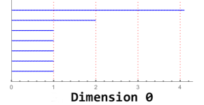
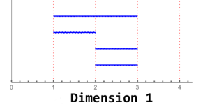
Let be the -th persistent homology of a filtration . For and , define that can be interpreted as the number of -dimensional homology classes which are “born” at time and “die” at time . Then, can be represented by the multiset444A multiset is a set whose elements can be repeated of intervals , called the -th persistence barcode or diagram of , where each interval appears times.
In this paper, we assume barcodes have a finite number of elements, find an example in Figure 2. We introduce now the notation used along the paper.
Notation 2.6.
Let denote the set of persistence barcodes. Given a persistence barcode , its intervals will be denoted by for . Besides, the length of will be denoted by , that is, . Finally, will denote the sum . Moreover, given two persistence barcodes and , denote by and by .
Let us define the following subsets of .
Definition 2.7.
The set of finite persistence barcodes is defined as:
The set of persistence barcodes whose intervals all start at is denoted as , that is:
And, finally, the set of normalized persistence barcodes is defined as:
In the sequel, we will assume that for all to avoid degenerate cases. There is a correspondence between persistence barcodes in and persistence barcodes in .
Definition 2.8.
Let be the projection defined as the composition: where and are defined as follows (see Figure 3):
The following metrics can be defined on .
Definition 2.9 (Wasserstein and bottleneck distances).
Let and . Define the -th Wasserstein distance as
where is any bijection between the multisets
and (including, if necessary, intervals of zero length) and is the cardinality555Since is a bijection, cardinality of refers to the number of elements of the domain of which coincides with the number of elements of the image of . of .
The limit case is called the bottleneck distance and is defined by
Observe that . Besides, in case or is then is set to . In case both and are then is set to . Notice also that we have replaced the and terms of the original definition of Wasserstein and bottleneck distance [7, p. 180-183] by and terms because, in this paper, persistence barcodes have always a finite number of intervals.
We finish this section with some well-known persistent homology stability results, supporting the idea that an algorithm designed using persistent homology tools will produce “similar” outputs for “similar” inputs.
Theorem 2.10 ([28]).
Let be two tame666The function is tame if there is a finite number of different elements in the set and such set consists of homology groups whose ranks are finite. Lipschitz functions on a metric space whose triangulations grow polynomially with constant exponent . Then, there are constants and such that the -th Wasserstein distance between their corresponding persistence barcodes, denoted by and , satisfies:
When , the constant is no longer necessary, obtaining the following most commonly used simplified version.
Corollary 2.11 ([7, p. 183]).
Let be a simplicial complex and be two monotonic functions. If and denote the corresponding persistence barcodes obtained from and , then
Finally, as a consequence of Theorem 2.10, we can assert the following.
Theorem 2.12 ([29]).
Consider two finite metric spaces , . Let be the two persistence barcodes obtained, respectively, from and . Then,
where denotes the Gromov-Hausdorff (GH) distance777The Gromov-Hausdorff distance between and is where is the Hausdorff distance between and and range over all the isometric embeddings of into some same metric space . .
Looking at these results, we can conclude that stability results are simpler when using the bottleneck distance than when using the Wasserstein distance.
3 Stability of persistent entropy
This section aims to show under which conditions persistent entropy is stable, which means that it is uniformly continuous or, more informally, there is a bound that “controls” the perturbation produced by noise in the input data. In the first subsection, we recall the definition of persistent entropy. Later, we provide several lemmas that will be needed to prove the stability of persistent entropy for finite persistence barcodes. Lastly, we will see how we can project persistence barcodes with infinite length intervals to finite persistence barcodes in a stable way. These projections will allow to provide general stability results for persistent entropy.
3.1 Persistent entropy
So far, we have seen how persistent homology can be represented using persistence barcodes in a stable way. Nevertheless, sometimes, we might prefer to use only a number to summarize persistent homology (such as persistent entropy), even if we are losing information by doing so.
Definition 3.1 (persistent entropy [12, 11]).
The persistent entropy of a persistence barcode in is defined as:
For simplicity of notation, will refer to the -base-2 function. Observe that, to compute persistent entropy, we only have to consider the length of each interval . The following immediate result holds.
Remark 3.2.
If then .
Let us see now a naive example of application of persistent entropy.
Example 3.3.
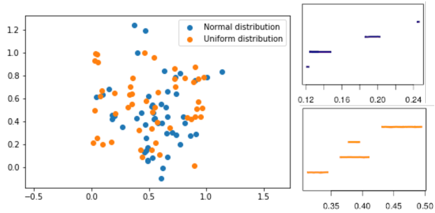
Suppose we have 20 point clouds: 10 point clouds following a normal distribution and 10 point clouds following a uniform distribution (see Figure 4). Note that since the sample is small, we should not perform a multivariate statistical test, so the idea is to perform univariate statistical tests using persistent entropy. Let us compute the -st persistent homology using the Vietoris-Rips filtration. Observe that the computed persistence barcodes will never have infinite length intervals since Vietoris-Rips complexes are always contractible from a (large enough) value. Now, let us compute the persistent entropy of each persistence barcode to obtain a number for each of the point clouds. Let us set and perform the Mann–Whitney U test888See [30] for a simple introduction to statistical tests.. We obtain a -value of for this experiment so and we can conclude that there are significant differences between the point clouds.
Note that, in the definition of persistent entropy, we assume that there are no infinite length intervals in the persistence barcode. We will study in Subsection 3.4 how to proceed when infinite length intervals appear.
3.2 Preliminary lemmas
In this subsection, we will provide several results useful to prove the main results in this paper that will be given in Subsection 3.3.
Let us recall a well-known result regarding -norms.
Remark 3.4.
Let and . Let and . If then .
The following result extends Remark 3.4 to the Wasserstein distance.
Lemma 3.5.
Let be the -th Wasserstein distance for persistence barcodes. If and then
Proof.
The result below states that when we translate the intervals of given persistence barcodes and to the origin by projection , the distance between them can be doubled.
Lemma 3.6.
If then
Proof.
Let be a bijection where is reached. Let denote the cardinality of . Since and then we have:
∎
To establish what we consider “big” or “small” error, we need to normalize the distances between persistence barcodes in some way.
Definition 3.7 (relative error).
Let and The relative error is defined as:
Observe that, according to Lemma 3.6, it is satisfied that
The next lemma is a technical result that we will use later.
Lemma 3.8.
Let be a bijection between the multisets . Let be the cardinality of . Then for all , , we have:
Proof.
Without loss of generality, suppose . Since
| (2) |
we consider two cases: and . In the first case:
For the second case (i.e., when ), use that to obtain:
∎
Let us now see how the projection affects the relationship between the relative error and the distance .
Lemma 3.9.
If and then
Proof.
Recall that if and then we have:
Let be a bijection where is reached, that is:
where is the cardinality of . Notice that or might be for some if intervals of zero length were needed for creating bijection . We can assume without loss of generality that . Now by Lemma 3.8 we have:
Applying Lemma 3.6 we have that
.
By Lemma 3.5, we get that
.
Finally, since we assumed that then
.
∎
3.3 Stability results for
Two important results about the stability of persistent homology were recalled in Section 2 (Theorem 2.10 and Theorem 2.12). These results guarantee that if two filter functions (or two metric spaces) are “similar”, then their corresponding persistence barcodes will be “similar” as well. Besides, there also exist stability results for Shannon entropy defined on probability distributions. To combine these results to prove stability of persistent entropy we need to adapt the last ones to the metric space of persistence barcodes.
First of all, recall that the continuity of persistent entropy with respect to the bottleneck distance is proven in [18]. The following proposition generalizes that result to the Wasserstein distance.
Proposition 3.10.
Let and let be the -th Wasserstein distance with . If we fix a maximum number of intervals and a minimum sum of the lengths of the intervals in a persistence barcode, then the persistent entropy is continuous on :
The stability of Shannon entropy has been previously studied by Lesche in [31] for the -norm due to its importance in physics. That bound can be slightly improved as shown in [32].
Theorem 3.11 ([32, p. 664]).
Let and be two finite probability distributions (seen as vectors in ), and let and be, respectively, their Shannon entropy. If then
Notice that the restriction is reasonable because is at most .
Now, let us introduce one of the main result of this paper. We can observe that since the space can be interpreted as finite probability distributions, we can first project the persistence barcodes of onto and then apply the previous theorem to obtain the desired stability result.
Theorem 3.12 (stability of persistent entropy).
Let . Let us assume that . Then:
Proof.
First, by Remark 3.2, we have that
| (3) |
Now, let be a bijection where is reached, that is,
where is the cardinality of . Let be the vector and the vector . Then, and by Lemma 3.9,
Now, since then . By Theorem 3.11 we have that
| (4) |
Now, since is increasing as long as and , since by assumption999See the comment after Notation 2.6., then
| (5) |
Finally,
since . ∎
Although the bound of can tend to for an arbitrary large for , the relative value is bounded when tends to since . In other words,
Table 1 shows some numerical examples regarding such relative value.
| 10 | 0.339794 | 0.2 | 0.115051 | 0.0539794 |
|---|---|---|---|---|
| 510 | 0.251631 | 0.136933 | 0.0740258 | 0.0325498 |
| 1010 | 0.246531 | 0.133285 | 0.0716526 | 0.0313102 |
| 1510 | 0.243975 | 0.131457 | 0.070463 | 0.0306888 |
| 2010 | 0.242321 | 0.130274 | 0.0696935 | 0.0302868 |
| 2510 | 0.24112 | 0.129415 | 0.0691346 | 0.0299949 |
| 3010 | 0.240187 | 0.128747 | 0.0687007 | 0.0297682 |
| 3510 | 0.239431 | 0.128206 | 0.0683486 | 0.0295843 |
| 4010 | 0.238798 | 0.127754 | 0.0680541 | 0.0294305 |
| 4510 | 0.238256 | 0.127366 | 0.067802 | 0.0292988 |
| 5010 | 0.237784 | 0.127028 | 0.0675823 | 0.029184 |
3.4 Persistence barcodes with infinite length intervals
In order to extend the definition of persistent entropy to persistence barcodes with infinite length intervals, it is common to define a projection from to that transforms infinite length intervals into finite length intervals. There are many ways to do this and depending on choice, persistent entropy may no longer be stable or scale-invariant. In this section, we explain some projections and their properties.
We start with a simple example. To avoid calculations involving the infinite value when computing persistent homology, usually, an upper bound is fixed and considered to be the infinite value. Then, if we want to compute persistent entropy, the first idea could be just to assign this upper bound to each of the infinite values that appear in the infinite length intervals.
Definition 3.13 (projection ).
Let . Define the projection such that for ,
The following result confirms that the projection is stable.
Proposition 3.14.
Let . Then, projection satisfies that
Proof.
Let and . Let be a bijection where is reached. Let denote the cardinality of . Observe that if and then . Nevertheless, if and (resp. and ) then . Finally, if then . We conclude:
∎
Despite being stable, is not scale-invariant. By definition, a projection is scale-invariant if , being the scalar multiplication of each of the intervals (notice that ). We now define the following stable and scale-invariant projections from to .
Definition 3.15 (projections , , ).
Let and . Let . Then:
-
•
where if and otherwise; being the maximum finite value for .
-
•
where if and otherwise; being where and .
-
•
where if and otherwise; being the maximum finite value for .
Notice that and both are equivalent to remove the infinite length intervals.
Proposition 3.16 (stability of projections , , ).
Given two persistence barcodes with the same number of infinite length intervals, we have that:
If the length of the longest finite interval in and are both greater than , then
Proof.
Sort the intervals of and such that their first intervals are the infinite length intervals and for , consider a bijection where is reached. Let denote the cardinality of . Let refer to , or . We have:
If then, for all , , we have:
Assume, without loss of generality, that . Then, the interval with length paired to an interval with length by bijection satisfies, by definition, that and then
obtaining
and
If then, for all , , we have:
By the reverse triangle inequality:
being the cardinal of a bijection where is reached. By Lemma 3.6,
and finally,
If then
We only have to prove that . By reduction to the absurd, suppose that . Without loss of generality, assume . Take one interval in with endpoint and another one in with endpoint . Since, by hypothesis, the length of both intervals is greater than then we can assume that they are not paired with the diagonal when computing the bottleneck distance. Let be the interval in paired with . Then
leading to a contradiction. Therefore,
∎
Of course, these projections are just a few of the many possible that can be defined. In the past, since persistent entropy only takes into account the length of the intervals, infinite length intervals were usually replaced by intervals of a fixed finite length. For example, in [14], was used plus a constant. With respect to this case, notice that adding a constant in the definition of any of the projections above will produce stable but not scale-invariant projections. In [16], infinite length intervals were ignored using the stable and scale-invariant projection obtaining a topological based variable for analyzing cell arrangement.
3.5 Stability results for
Let us now introduce the following results on the stability of persistent entropy for the general case. For simplicity, we have removed infinite length intervals using for these statements, but we could use any other stable projection to remove such intervals. This way, the formulas that appear in the statements below would change according to the inequalities of Proposition 3.16.
Theorem 3.17.
Let be a simplicial complex and let be two monotonic functions. Let be their corresponding persistence barcodes. If then
where , being (resp. ) the number of intervals of (resp. ).
Proof.
Theorem 3.18.
Let be the persistence barcodes obtained respectively from and , being and two finite metric spaces. If then,
where , being (resp. ) the number of intervals of (resp. ).
Proof.
It seems appropriate now to recapitulate the results of this section before moving on. As shown in the following diagram, at the beginning of the section we wanted to prove implication (A). In order to do it, we separated the problem into three parts ((1), (2) and (3)):
4 Entropy-based summary functions
As we have already mentioned, numbers summarizing persistence barcodes (such as persistent entropy) are very useful to perform statistical tests. Nevertheless, if we want to perform a classification task, their discriminatory power might not be enough. One of the possible solutions is to summarize persistence barcodes using functions. Summary functions (such as he already mentioned persistence silhouettes, Euler characteristic curves, topological intensity maps or persistence landscapes) have been used in the past to obtain statistical information from persistence barcodes. For example, a simple but effective way of summarizing a persistence barcode is the Betti curve defined as follows: If then
That is, is the number of intervals in which are “alive” at time .
In this section, we will define a new summary piece-wise constant function (also known as step function). It is similar to the Betti curve but uses persistent entropy instead of Betti numbers. We will prove its stability and show examples where such function measures different features of the persistence barcode than the Betti curve. Besides, and contrary to what happened with persistent entropy, we will see that the normalization of this function is also stable.
4.1 Entropy summary function (ES-function)
We now define a new function that pairs a persistence barcode with a real-valued piece-wise constant function. This new function summarizes information about the number of intervals of a given persistence barcode and their homogeneity and, as we will prove at the end of this subsection, is stable with respect to the bottleneck distance.
Definition 4.1 (ES-function).
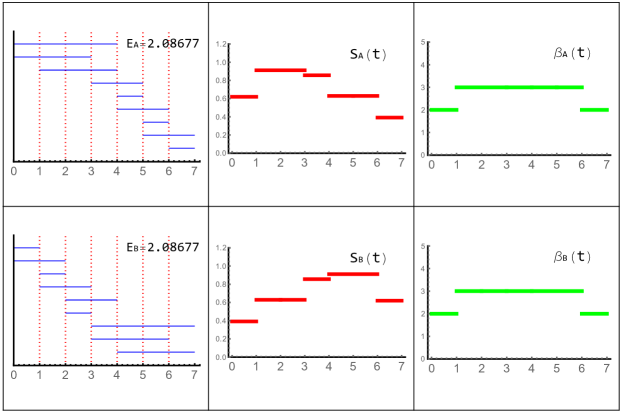
The entropy summary function (ES-function) of a persistence barcode in is the real-valued piecewise linear function:
where if and otherwise.
In other words, the ES-function pairs a persistence barcode and an instant with the partial sum of corresponding to the intervals of that are “alive” at that moment , that is, . See Figure 5. Notice that and , being the space of real-valued piece-wise constant functions.
The following result states that the ES-function is stable with respect to the bottleneck distance.
Theorem 4.2 (stability of the ES-function).
Let be the ES-function, the bottleneck distance and two persistence barcodes in . Let be the cardinality of a bijection, denoted as , where is reached. If then:
 |
 |
Proof.
Denote the expression by . Then,
Let us now compute a bound for . Without loss of generality, assume that . Since represents the length of the intersection of non-null paired intervals, we have that
| (6) |
Let us compute a bound for . Denote the expression by . By Lemma 3.8 and Lemma 3.9, we have that
| (7) |
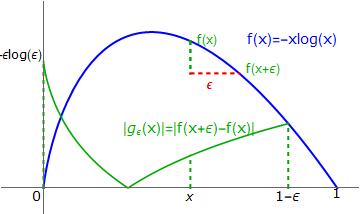
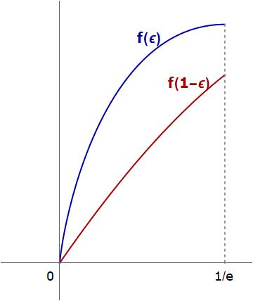
By hypothesis, we have that , so . Then, . Now, recall that is continuous and concave in with and consider the function defined for any . As is concave and differentiable in , is decreasing, is negative and so is decreasing monotone. Therefore the maximum of its absolute value is attained at one of the extreme points of the interval . Observe that since , this maximum is reached at (see Figure 6):
| (10) |
Now, using (10), we obtain that:
| (11) |
Due to (4.1) and being increasing in , we obtain from (11) that:
| (12) |
Finally, by (6) and (12), we have:
| (13) |
Now, let us compute a bound for
Consider the function . Its integral gives the “period of time” in which the -th interval of , , is “alive” and the -th interval of , , is not. This might happen in both the initial and the end of the intervals. Therefore, if then:
We also have that, in the case where , the period of time where the -th interval of is alive and the one of is not, is null. Therefore
and vice-versa. Using both previous statements and that we can deduce:
From this last equation and (13), we obtain the desired result. ∎
Notice that the ES-function is based on persistent entropy whereas the Betti curve consists of counting the number of “alive” intervals. Both functions (the ES-function and the Betti curve) are continuous with respect to the bottleneck distance if the maximum number of intervals is fixed. Nevertheless, the ES-function is expected to perform better than the Betti curve in a noisy context since persistent entropy is stable while counting the number of intervals is not, even if it is continuous.
4.2 Normalized entropy summary function (NES-function)
One of the main aims of persistent homology is to represent the shape of the input data. In some applications, like image analysis or material science (see [33] for a review), it may be important to detect some repetitive pattern independently of the size of the input dataset. A possible tool to do this is a normalized version of the summary function, in order to try to capture the shape of the space and not the size.
Definition 4.3 (NES-function).
The normalized entropy summary function (NES-function) of a persistence barcode in is defined as:
Like the ES-function, this function is also stable.
Theorem 4.4 (Stability of the NES-function).
Under the same hypothesis as in Theorem 4.2, we have that:
Proof.
5 Experimentation
Our summary functions have been recently applied to real-world data in [34] and [35]. The authors of these papers explicitly mentioned the stability of these functions, presented here and in the arXiv version [36], to guarantee the robustness of their methods. In [34] an algorithm is developed for segmenting and classifying different types of skin lesions in a given skin image. The database used is the International Skin Imaging Collaboration (ISIC) dataset101010https://www.isic-archive.com consisting of 10015 skin lesson images. In the classification part, the authors first computed the persistence diagram for each channel of the image in different color space. Then, topological features including our ES-function (referred as “persistent entropy curves”) and Betti curves were calculated from persistence diagrams obtained previously. Finally, the authors used multi-class support vector machine with a “one-against-one” strategy. The best 3 scores they had on the validation set was 65.6%, 66%, and 67.2% depending on the color space used. Besides, in [35], the authors developed a general framework called “persistence curves” for vectorizing persistence diagrams inspired in our ES-function, referred in [35] as “life entropy”, denoted by , and used for texture classification on four different texture datasets. They showed that a combination of different flavors of persistence curves (including our ES-function) produces the best result, showing that they are complementary to each other.
This section is devoted to experiments. In Subsection 5.1 we study how the NES-function and similar vectorizations such as the Betti curves and the persistence silhouettes may benefits from each other in machine learning tasks. The dataset considered in our experiment consists of miscellaneous real-world images taken from the USC-SIPI Image Database111111http://sipi.usc.edu/database/database.php?volume=misc. The machine learning method used in our experiment is the random forest technique [37]. Later, in Subsection 5.2, we will also add persistence images to our experiment to see how different vectorization methods perform depending on the nature of the data sets. In particular, we will consider the Flickr Material Database (FMD)121212https://people.csail.mit.edu/celiu/CVPR2010/FMD/. The whole experiment has been developed in Python and R. Scripts and notebooks can be downloaded from here131313https://github.com/Cimagroup/New-Summary-Function-For-TDA. Libraries used are scikit-TDA141414https://scikit-tda.org/ (in particular Persim151515https://persim.scikit-tda.org/ and Ripser161616https://ripser.scikit-tda.org/), scikit-image171717https://scikit-image.org/, scikit-learn181818https://scikit-learn.org/ and R-TDA-package191919https://cran.r-project.org/web/packages/TDA/index.html.
5.1 USC-SIPI dataset experiment
| Betti curve | NES-function | Silhouette | Silouette | |
|---|---|---|---|---|
| Gauss | 0.198 | 0.114 | 0.039 | 0.024 |
| Poisson | 0.245 | 0.200 | 0.156 | 0.086 |
| S&P | 0.140 | 0.296 | 0.424 | 0.459 |
| Betti curve | NES-function | Silhouette | Silhouette |
|---|---|---|---|
| 0.913 | 0.672 | 0.500 | 0.354 |
We have followed this procedure:
-
Step 1.Transform the images to gray scale.
Step 2. Add Gaussian, Poisson and salt-and-pepper noise to the data.
Step 3. Compute persistence diagrams using lower-start filtration.
Step 4. Summarize the diagrams using some vectorization method: the Betti curve, the NES-function or the persistence silhouettes.
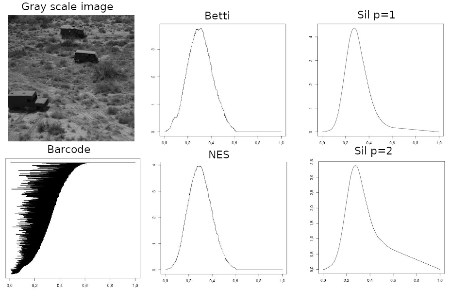
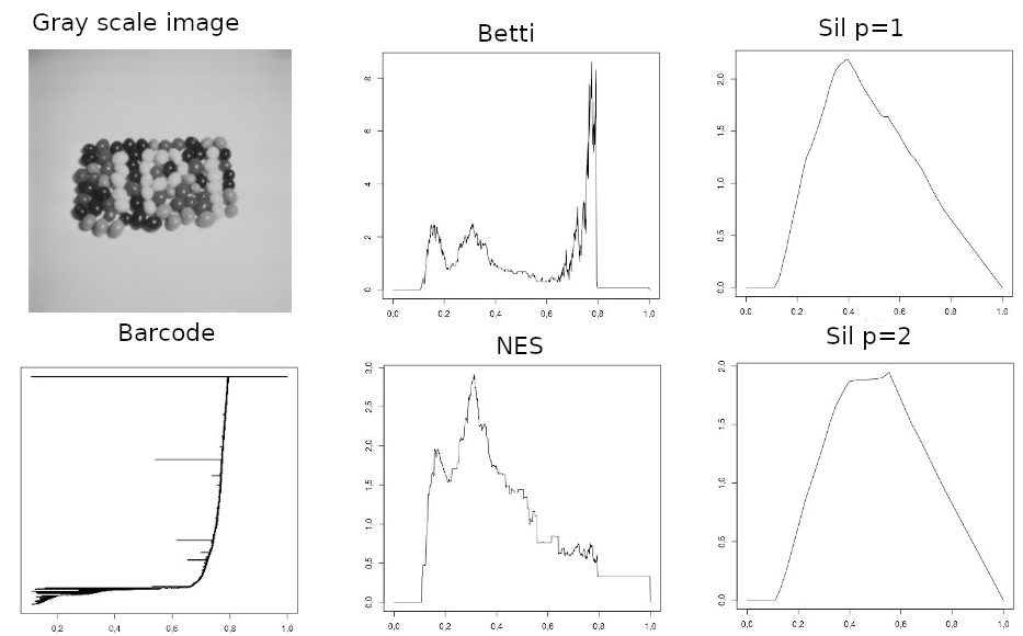
Let us compare the results obtained. First, the computational time was very similar to obtain all of them so we have omitted it from the analysis. A first conclusion is that for some images like the one in Figure 7, the outputs have extremely similar shapes while in others, like the one in Figure 8, the outputs have completely different shapes, showing that these functions may provide complementary information regarding different aspects of the same image. Robustness results have been obtained computing the -distance of each summary function on clean and noisy images, see Table 2. Observe that the results obtained for the NES-function is always between those obtained for the Betti curve and the persistence silhouettes. The Betti curve only performs better for salt-and-pepper noise. This fact is expected since persistence diagrams together with the bottleneck distance are unstable to salt-and-pepper noise when they are calculated using the lower-star filtration. It tells us that the NES-function and the persistence silhouettes are more robust to stastistical noise than the Betti curve. However, the Betti curve is more robust to impulsive noise.
We have also pairwise compared all the clean images for each summary function using the -distance and, as expected, since all images in the database are different in nature, this value is high, see Table 3.
We can conclude that the NES-function is usually more discriminative than the persistence silhouettes but less than the Betti curve. Nevertheless, these functions may provide information regarding different aspects of the same image and therefore may complement each other as it is shown in the next subsection.
5.2 FMD dataset experiment
First, we have transformed the given color images to gray scale images and computed their lower-start filtration. In a first part of this experiment, we have computed the Betti curve, the NES-function and the persistence silhouette for . Materials in the FMD database are classified in ten categories: 0-foliage, 1-glass, 2-leather, 3-metal, 4-paper, 5-plastic, 6-stone, 7-water, 8-wood and 9-fabric. Then, we have applied the random forest technique to classify the images using the output of the summary functions. Results are shown in Table 4. Note that the one that performs best is the combination of the Betti curve and the NES function. Besides, the persistence silhouettes also improve their performance when combined with the NES-function.
| Betti | Silhouette | Nes | B + S | B + N | S + N | B + S + N |
|---|---|---|---|---|---|---|
| 0.285 | 0.185 | 0.24 | 0.285 | 0.29 | 0.25 | 0.265 |
In a second part of this experiment, we want to illustrate that, depending on the data, some methods may perform better than others. This is the reason why this time we do not combine functions. The idea is to try to distinguish categories in the database when compared pairwise. We have performed 45 tests, one for each pair of materials. We have added another popular vectorization method: persistence images (with pixels). Results are shown in Table 5 where best marks have been highlighted.
| 0vs1 | 0vs2 | 0vs3 | 0vs4 | 0vs5 | 0vs6 | 0vs7 | 0vs8 | 0vs9 | |
|---|---|---|---|---|---|---|---|---|---|
| B | 0.6 | 0.675 | 0.7 | 0.6 | 0.575 | 0.725 | 0.675 | 0.8 | 0.775 |
| S | 0.625 | 0.525 | 0.55 | 0.45 | 0.55 | 0.75 | 0.575 | 0.775 | 0.675 |
| N | 0.5 | 0.6 | 0.7 | 0.5 | 0.45 | 0.725 | 0.7 | 0.8 | 0.775 |
| PI | 0.55 | 0.725 | 0.8 | 0.675 | 0.6 | 0.775 | 0.875 | 0.85 | 0.825 |
| 1vs2 | 1vs3 | 1vs4 | 1vs5 | 1vs6 | 1vs7 | 1vs8 | 1vs9 | 2vs3 | |
| B | 0.8 | 0.55 | 0.75 | 0.75 | 0.725 | 0.575 | 0.65 | 0.575 | 0.475 |
| S | 0.825 | 0.65 | 0.8 | 0.6 | 0.75 | 0.475 | 0.775 | 0.6 | 0.45 |
| N | 0.85 | 0.6 | 0.775 | 0.75 | 0.775 | 0.625 | 0.675 | 0.675 | 0.5 |
| PI | 0.85 | 0.775 | 0.775 | 0.675 | 0.875 | 0.575 | 0.625 | 0.675 | 0.6 |
| 2vs4 | 2vs5 | 2vs6 | 2vs7 | 2vs8 | 2vs9 | 3vs4 | 3vs5 | 3vs6 | |
| B | 0.825 | 0.7 | 0.7 | 0.525 | 0.65 | 0.65 | 0.725 | 0.925 | 0.825 |
| S | 0.725 | 0.575 | 0.5 | 0.5 | 0.6 | 0.55 | 0.675 | 0.65 | 0.6 |
| N | 0.725 | 0.65 | 0.55 | 0.475 | 0.65 | 0.75 | 0.7 | 0.85 | 0.625 |
| PI | 0.8 | 0.8 | 0.625 | 0.625 | 0.575 | 0.7 | 0.65 | 0.775 | 0.775 |
| 3vs7 | 3vs8 | 3vs9 | 4vs5 | 4vs6 | 4vs7 | 4vs8 | 4vs9 | 5vs6 | |
| B | 0.7 | 0.625 | 0.725 | 0.55 | 0.825 | 0.725 | 0.625 | 0.55 | 0.65 |
| S | 0.625 | 0.6 | 0.675 | 0.625 | 0.7 | 0.65 | 0.45 | 0.6 | 0.6 |
| N | 0.7 | 0.65 | 0.725 | 0.55 | 0.75 | 0.725 | 0.6 | 0.65 | 0.725 |
| PI | 0.6 | 0.725 | 0.675 | 0.625 | 0.775 | 0.775 | 0.65 | 0.625 | 0.6 |
| 5vs7 | 5vs8 | 5vs9 | 6vs7 | 6vs8 | 6vs9 | 7vs8 | 7vs9 | 8vs9 | |
| B | 0.85 | 0.7 | 0.8 | 0.9 | 0.825 | 0.8 | 0.875 | 0.65 | 0.9 |
| S | 0.7 | 0.7 | 0.625 | 0.625 | 0.675 | 0.675 | 0.7 | 0.7 | 0.575 |
| N | 0.7 | 0.675 | 0.675 | 0.775 | 0.775 | 0.725 | 0.7 | 0.7 | 0.625 |
| PI | 0.825 | 0.725 | 0.55 | 0.7 | 0.775 | 0.675 | 0.725 | 0.725 | 0.625 |
6 Conclusions and future work
In this paper, the stability of persistent entropy is provided justifying its application as an useful statistic in topological data analysis. What is more, persistent entropy has been used to define an stable summary function, the ES-function, and its normalised version, the NES-function. We have shown that, in general, they perform better than the Betti curve in noisy context and that they can be useful for machine learning tasks.
Several types of persistence curves inspired in our persistent entropy summaries were also defined by Y.M Chung and A. Lawson in [35]. They also corroborate the idea that such persistence functions are somehow complementary and combined provide a classification performance comparable to the state of the art. Together with Y.M. Chung and A. Lawson we plan to apply our summary functions to other higher dimensional non-image dataset such as, for example, the TOSCA dataset of 3D meshes202020http://tosca.cs.technion.ac.il/book/resources_data.html. Besides, as a future work,
it would be interesting to
deeply
compare these and other summary functions with other topological vectorization methods
existing in the literature.
Acknowledgments: We would like to thank the reviewers for their very valuable comments and suggestions. The third author has been partially funded by VI-PPITUS (University of Seville).
References
- [1] M. Mrozek, M. Żelawski, A. Gryglewski, S. Han, and A. Krajniak, “Homological methods for extraction and analysis of linear features in multidimensional images,” Pattern Recognit., vol. 45, no. 1, pp. 285 – 298, 2012.
- [2] S. Biasotti, D. Giorgi, M. Spagnuolo, and B. Falcidieno, “Size functions for comparing 3d models,” Pattern Recognit., vol. 41, no. 9, pp. 2855 – 2873, 2008.
- [3] M. Ferri, “Persistent topology for natural data analysis — a survey,” Towards Integrative Machine Learning and Knowledge Extraction. Lecture Notes in Computer Science. Springer, vol. 10344, no. 2, pp. 127–139, 2017.
- [4] G. Carlson, A. Zomorodian, A. Collins, and L. Guibas, “Persistence barcodes for shapes,” Int. Journal of Shape Modeling, vol. 11, no. 02, pp. 149–187, 2005.
- [5] H. Edelsbrunner, D. Letscher, and A. Zomorodian, “Topological persistence and simplification,” Discrete Comput. Geom., vol. 28, no. 4, pp. 511–533, 2002.
- [6] P. Bubenik, “Statistical topology using persistence landscapes,” J. Mach. Learn. Res., vol. 16, pp. 77–102, 2015.
- [7] H. Edelsbrunner and J. Harer, Computational Topology: An Introduction. American Mathematical Society, 2010.
- [8] N. Otter, M. Porter, U. Tillmann, P. Grindrod, and H. Harrington, “A roadmap for the computation of persistent homology,” Entropy, vol. 17, no. 6, 2017.
- [9] Y. Mileyko, S. Mukherjee, and J. Harer, “Probability measures on the space of persistence diagrams,” Inverse Problems, vol. 27, no. 12, p. 124007, 2011.
- [10] C. Shannon, “A mathematical theory of communication,” Bell System Technical Journal, vol. 27, no. 3, pp. 379–423, 1948.
- [11] M. Rucco, F. Castiglione, E. Merelli, and M. Pettini, “Characterisation of the idiotypic immune network through persistent entropy,” in Proceedings of ECCS 2014, pp. 117–128, 2014.
- [12] H. Chintakunta, T. Gentimis, R. Gonzalez-Diaz, M. J. Jimenez, and H. Krim, “An entropy based persistence barcode,” Pattern Recognit., vol. 48, no. 2, pp. 391–401, 2015.
- [13] E. Merelli, M. Piangerelli, M. Rucco, and D. Toller, “A topological approach for multivariate time series characterization: the epileptic brain,” EAI Endorsed Transactions on Self-Adaptive Systems, vol. 16, no. 7, 2016.
- [14] M. Rucco, R. Gonzalez-Diaz, M. Jimenez, N. Atienza, and et al, “A new topological entropy-based approach for measuring similarities among piecewise linear functions,” Signal Process, vol. 134, pp. 130–138, 2017.
- [15] J. Binchi, E. Merelli, M. Rucco, G. Petri, and F. Vaccarino, “jholes: A tool for understanding biological complex networks via clique weight rank persistent homology,” Electron. Notes Theor. Comput. Sci., vol. 306, pp. 5–18, 2014.
- [16] N. Atienza, L. Escudero, M. Jimenez, and M. Soriano-Trigueros, “Persistent entropy: a scale-invariant topological statistic for analyzing cell arrangements,” Unpublished, vol. abs/1902.06467, 2019.
- [17] X. Wang, F. Sohel, M. Bennamoun, Y. Guo, and H. Lei, “Scale space clustering evolution for salient region detection on 3d deformable shapes,” Pattern Recognit., vol. 71, pp. 414 – 427, 2017.
- [18] N. Atienza, R. Gonzalez-Diaz, and M. Rucco, “Persistent entropy for separating topological features from noise in vietoris-rips complexes,” J. Intell. Inf. Syst., vol. 52, no. 3, pp. 637–655, 2019.
- [19] J. Reininghaus, S. Huber, U. Bauer, and R. Kwitt, “A stable multi-scale kernel for topological machine learning,” in 2015 IEEE Conference on Computer Vision and Pattern Recognition (CVPR), pp. 4741–4748, 2015.
- [20] G. Kusano, K. Fukumizu, and Y. Hiraoka, “Persistence weighted gaussian kernel for topological data analysis,” in Proc. of the 33rd Int. Conf. on Machine Learning, vol. 48, p. 2004–2013, 2016.
- [21] M. Carrière, M. Cuturi, and S. Oudot, “Sliced Wasserstein kernel for persistence diagrams,” in Proc. of the 34th Int. Conf. on Machine Learning (D. Precup and Y. W. Teh, eds.), vol. 70, pp. 664–673, 2017.
- [22] F. Chazal, B. Fasy, F. Lecci, A. Rinaldo, and L. Wasserman, “Stochastic convergence of persistence landscapes and silhouettes,” J. Comput. Geom., vol. 6, no. 2, p. 140–161, 2015.
- [23] H. Adams, T. Emerson, M. Kirby, R. Neville, and et al., “Persistence images: A stable vector representation of persistent homology,” J. Mach. Learn. Res., vol. 18, no. 8, pp. 1–35, 2017.
- [24] E. Richardson and M. Werman, “Efficient classification using the euler characteristic,” Pattern Recognit. Lett., vol. 49, pp. 99–106, 2014.
- [25] P. Pranav, H. Edelsbrunner, R. van de Weygaert, G. Vegter, and et al., “The topology of the cosmic web in terms of persistent betti numbers,” Mon. Not. R. Astron. Soc., vol. 465, no. 4, pp. 4281–4310, 2017.
- [26] B. Rieck, F. Sadlo, and H. Leitte, “Topological machine learning with persistence indicator functions,” in Topological Methods in Data Analysis and Visualization V, Springer International Publishing, to appear.
- [27] Y. Umeda, “Time series classification via topological data analysis,” Trans. Japan Soc. Artificial Intelligence, vol. 32, no. 3, pp. D–G72_1–12, 2017.
- [28] D. Cohen-Steiner, H. Edelsbrunner, J. Harer, and Y. Mileyko, “Lipschitz functions have -stable persistence,” Found. Comput. Math., vol. 10, no. 2, pp. 127–139, 2010.
- [29] F. Chazal, D. Cohen-Steiner, L. Guibas, F. Mémoli, and S. Oudot, “Gromov-hausdorff stable signatures for shapes using persistence,” Comput. Graphics Forum, vol. 28, no. 5, p. 1393–1403, 2009.
- [30] G. Dallal, The Little Handbook of Statistical Practice. Amazon Digital Services LLC, 2012.
- [31] B. Lesche, “Instabilities of rényi entropies,” J. Stat. Phys., vol. 27, no. 2, pp. 419–422, 1982.
- [32] T. Cover and J. Thomas, Elements of Information Theory. Wiley Series in Telecommunications and Signal Processing, 2nd ed., 2006.
- [33] M. Buchet, Y. Hiraoka, and I. Obayashi, “Persistent homology and materials informatics,” in Nanoinformatics, pp. 75–95, Springer, Singapore, 2018.
- [34] Y. Chung, C.-S. Hu, A. Lawson, and C. Smyth, “Topological approaches to skin disease image analysis,” in 2018 IEEE Int. Conf. on Big Data, 2018.
- [35] Y. Chung and A. Lawson, “Persistence curves: A canonical framework for summarizing persistence diagrams,” Unpublished, vol. abs/1904.07768, 2019.
- [36] N. Atienza, R. Gonzalez-Diaz, and M. Soriano-Trigueros, “On the stability of persistent entropy and new summary functions for TDA,” Unpublished, vol. abs/1803.08304, 2018.
- [37] L. Breiman, “Random forests,” Mach. Learn., vol. 45, p. 5–32, 2001.