Very fast stochastic gravitational wave background map-making using folded data
Abstract
A stochastic gravitational-wave background (SGWB) is expected from the superposition of a wide variety of independent and unresolved astrophysical and cosmological sources from different stages in the evolution of the Universe. Radiometric techniques are used to make sky maps of anisotropies in the SGWB by cross-correlating data from pairs of detectors. The conventional searches can be made hundreds of times faster through the folding mechanism introduced recently. Here we present a newly developed algorithm to perform the SGWB searches in a highly efficient way. Taking advantage of the compactness of the folded data we replaced the loops in the pipeline with matrix multiplications. We also incorporated well-known HEALPix pixelization tools for further standardization and optimization. Our Python-based implementation of the algorithm is available as an open source package PyStoch. Folding and PyStoch together has made the radiometer analysis a few thousand times faster; it is now possible to make all-sky maps of a stochastic background in just a few minutes on an ordinary laptop. Moreover, PyStoch generates a skymap at every frequency bin as an intermediate data product. These techniques have made SGWB searches very convenient and will make computationally challenging analyses like blind all-sky narrowband search feasible.
pacs:
04.80.Nn, 95.55.Ym, 98.70.VcI Introduction
A new era in astronomy began with the detection of gravitational waves (GW) Abbott et al. (2016a). As was anticipated, the first detected sources are all compact binary coalescence Abbott et al. (2016b, 2017a, 2017b, 2017c, 2017d). GW astronomy, however, promises much more excitement. A vigorous global effort is underway to observe GW signals in widely separated frequency bands. This includes ground-based interferometric detectors aLIGO, aVIRGO, GEO, TAMA, KAGRA Collaboration et al. (2015); Acernese et al. (2015); Affeldt et al. (2014); Ando and the TAMA collaboration (2002); Somiya (2012), pulsar timing arrays Hobbs et al. (2010), and the planned space-based detectors such as LISA, DECIGO, BBO Amaro-Seoane et al. (2013); Seiji Kawamura et al. (2011); Harry et al. (2006). Different kinds of sources Einstein (1918); Misner et al. (1973); Thorne (1987) are expected to be seen in the current and future generation network of detectors, the stochastic background being one of the most interesting ones. A stochastic background of gravitational waves (SGWB) Regimbau and Mandic (2008); Coward and Regimbau (2006) can be generated by the superposition of a wide variety of independent and unresolved astrophysical and cosmological sources from different stages in the evolution of the universe. The unresolved compact binary coalescence consisting of black holes and neutron stars, spinning neutron stars, supernovae, cosmic strings, inflationary models, phase transitions, and the pre-Big-Bang scenario are some of these sources which contribute towards this background Allen (1996); Grishchuk (2001); Turner (1997); Dhurandhar et al. (2011); Mazumder et al. (2014); Geller et al. (2018); Jenkins and Sakellariadou (2018). The background is likely to be anisotropic if it is dominated by the nearby universe Mazumder et al. (2014); Allen and Ottewill (1997). The detection of an anisotropic SGWB will offer novel opportunities to study the origin, distribution, and properties of various astrophysical objects, which are still not accessible to the current observational windows of astronomyAllen (1996, 1988); Sesana et al. (2008).
Various techniques have been developed to search for isotropic and anisotropic SGWB in data from detectors in different bands Romano and Cornish (2017). For GW detectors, since noise in geographically far away detectors are likely to be uncorrelated, data from pairs of detectors are cross-correlated to look for a stochastic signal Michelson (1987); Christensen (1992); Flanagan (1993); Allen and Ottewill (1997); Allen and Romano (1999); Cornish (2001). To probe anisotropies of the SGWB using ground-based detectors, the standard technique presently is the GW radiometer algorithm Lazzarini and Weiss (2004); Ballmer (2006); Mitra et al. (2008), which is analogous to aperture synthesis often used in radio astronomy Thompson et al. (2001); Ryle and Hewish (1960). The algorithm has been thoroughly studied and implemented in a pixel Ballmer (2006); Mitra et al. (2008) and spherical harmonic basis Thrane et al. (2009), where appropriate time-varying phase delays are applied to probe various spatial scales, and is routinely applied to LIGO data Aasi et al. (2014); Abbott et al. (2009, 2007a); Abadie et al. (2011); Abbott et al. (2007b). GW can also cause a considerable amount of perturbations in the time of arrival of pulses from millisecond pulsars. Efforts are on to measure these perturbations for some of the well modelled pulsars Mingarelli et al. (2013); Taylor and Gair (2013); Taylor et al. (2015) to constrain stochastic background in the nano-Hertz band, as well as, to probe the anisotropy of the background Gair et al. (2015).
In a recent work, the efficiency of the GW radiometer algorithm was dramatically improved through the mechanism of data folding Ain et al. (2015). A temporal symmetry in the GW radiometry algebra was utilized to fold the entire data into one sidereal day, thereby reducing the computational cost by a factor equal to the total number of days of observation. The enormous efficiency brought by folded data allows one to perform new kinds of analyses on long duration signals observed by ground based detectors using much lower computational resources, e. g., a blind all-sky narrowband search Thrane et al. (2015). A parallel pipeline developed to implement folding on LIGO data, and the advantages gained from that are well documented Ain et al. (2015).
However, folding does not exhaust the possibilities for computational improvement of the radiometer analysis. Here we present steps that can boost the efficiency of the algorithm by another factor of few tens. Moreover, the existing implementation of the stochastic pipeline is not equipped to take full advantage of folded data. Since the folded data volume is generally between 1-10 GB, the whole dataset can be loaded into a computer’s RAM, thereby dramatically reducing disk access and providing huge I/O advantage.
The scope for improvement is not limited to computational cost and associated conveniences. The current searches for an anisotropic SGWB in LIGO-Virgo data either use a spherical harmonic basis Abadie et al. (2011), which is appropriate for smooth and diffuse sources, but has limited sensitivity for localized sources like a galaxy cluster, or a pixel space radiometer search on a Cartesian grid. However, analysis of an equal area pixelization scheme is highly desirable for an all-sky map-making application like ours, primarily for better handling of noise in every pixel. Here we present the first implementation of radiometer search that is fully integrated with the Hierarchical Equal Area isoLatitude Pixelization of the sphere (HEALPix) scheme Gorski et al. (2005), which is perhaps the most widely-used pixelization scheme in astronomy at present for describing all-sky maps and has been rigorously tested by the cosmology community. Apart from the advantages of equal area pixels, HEALPix offers highly efficient tools for Fourier transforms on the sky, making it easy to transform a map from pixel to spherical harmonic bases and vice-versa, thus making the analysis suitable for both localised and diffused sources111However it is important to note that in practice, the final results (e.g., clean map, upper limit map, etc.) do depend on the chosen basis because of the different kinds of numerical errors associated with the inversion of the Fisher information matrices in different bases..
Finally, the existing LIGO-Virgo stochastic pipeline is suitable for broadband searches or targeted narrowband searches. The directional upper limits on GW intensity using data from the first Advanced LIGO observing run (O1) has been calculated Abbott et al. (2017e). With the fast tools in hand, we wanted to design the implementation in such a way that the intermediate results, the observed maps at every frequency bin, should be derivable in a straightforward way, which can then be combined to get the broadband result. This would also alleviate the need to perform separate searches for different spectral shapes of the modeled power spectral densities of the sources.
This paper is organized as follows. We briefly review the GW radiometer formalism as well as the folding method in Sec. II. Algorithms used in PyStoch and the narrowband map-making process are explained in Sec. III. Implementation of PyStoch and the results are presented in Sec. IV. We conclude the paper with a summary and discussion of algorithm performance in Sec.V along with results from simulated data, whose noise characteristics are statistically identical to that of O1 data.
II Mapping the Stochastic Gravitational Wave Background
II.1 Gravitational wave radiometer
Detectors which are geographically separated by vast distances are expected to have nearly statistically independent noise. Moreover, since a Gaussian stochastic background is characterized by its second moment, weighted cross-correlation of data from two independent detectors turns out to be the optimal statistic for detecting and mapping a SGWB Allen and Romano (1999); Mitra et al. (2008). The GW radiometer algorithm is based on this fundamental principle, which is commonly used to search for an isotropic or anisotropic SGWB in data from the ground-based interferometric detectors.
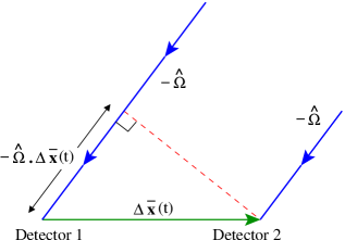
The GW radiometer algorithm considers the delay in the GW signal arrival at detectors which are at different locations. For a given direction in the sky, this delay changes as the baseline orientation changes due to the Earth’s rotation. If the time delayed data from two detectors are cross-correlated, the potential GW signals arriving from the given direction interfere constructively while the noises do not. When integrated over a long observational time, the signal cross-correlation grows faster than the noise variance, making the detection statistic more and more significant. The changes mentioned above in baseline orientation due to the Earth’s rotation allows one to construct an SGWB map by performing the synthesis for each direction in the sky, with an appropriate choice of the size of the pixel, even with only two detectors.
The working principle can be explained with the help of Fig 1. Consider two gravitational wave detectors denoted by and . The output data from the detectors can be written as,
| (1) | |||||
| (2) |
where and denote the gravitational wave strain in the two detectors due to the SGWB, and and denote the noises intrinsic to the first and second detectors respectively. Since the response of a detector (i.e., its antenna pattern with respect to the sky) changes with time, it is convenient to split the data taken from the detectors (time series data) into chunks of duration , such that is much greater than the light-travel time between the detectors, but small enough so that the detector response functions do not change considerably over that period. The typically acceptable chunk sizes are a few tens to a few hundreds of seconds. The Fourier transform of such a data segment, often called a short-term Fourier transforms (SFTs), is defined as,
| (3) |
where a tilde above a variable denotes its Fourier transform of a time series. As mentioned before, the noise in different geographically distant detectors can be assumed to be mutually uncorrelated and also uncorrelated with the signal. Thus we have,
| (4) | |||
| (5) |
The cross-power spectral density (CSD) of data, , from a baseline constituted by two detectors and and its noise component are given by,
| (6) | |||||
| (7) |
In the small signal limit, , the instantaneous cross-power noise variance becomes,
| (8) |
where are the one-sided power spectral density (PSD) of noise for a segment at time and is the duration of a segment.
The SGWB is characterized by the CSD of the signal. A search for anisotropic SGWB for a specific spectral distribution (assuming that the frequency spectral shape is the same in every direction of the sky) boils down to estimation of the SGWB skymap that is proportional to the flux coming from different directions on the sky Mitra et al. (2008). One can however perform the search in different set of basis on the two-sphere, in which the anisotropy map can be expanded as,
| (9) |
Then the expectation value of the CSD for a baseline can be written as Thrane et al. (2009)
| (10) |
where is is a geometric factor usually known as the overlap reduction function (ORF) defined as Christensen (1992); Finn et al. (2009),
| (11) |
where is the separation vector between the two detectors and denotes the antenna pattern functions of the detectors. Thus the observed CSD is a convolution of the SGWB skymap with the kernel , plus an additive noise term ,
| (12) |
Here , the kernel or the beam function is defined as,
| (13) |
The convolution equation has a standard maximum-likelihood (ML) solution which produces the estimates for the SGWB skymaps Mitra et al. (2008),
| (14) |
where , the dirty map, is given as,
| (15) |
and , the Fisher information matrix, as,
| (16) |
ML estimation of the convolution equation [Eq. (12)] takes the simple form given in Eq. (14) only when the inverse of the beam matrix exists. So directly inverting the beam matrix is non-trivial. Hence we prefer to solve the linear algebraic equation
| (17) |
to find , the ML estimate for the GWB sky map222Fisher information matrix in most cases is not easily invertible. And, due to the noise term in Eq. (12), the solution of Eq. (17) is noisy. A conjugate gradient or least square method is used to find the best ‘clean’ map ..
II.2 Folding
As we mentioned previously, gravitational wave radiometry relies on the basic principles of Earth rotation image synthesis. Characteristic properties of the SGWB and the algebra of analysis technique reveal that there exists a temporal symmetry. In the expressions for the dirty map in Eq. (15) and the Fisher information matrix in Eq. (16), the only two quantities needed for ML estimation of , the geometric part has a period of one sidereal day (i.e. 23 hr 56 min 4 sec). One can use this property to fold the entire detector data of several hundreds of days to only one sidereal day Ain et al. (2015). This can be done by splitting the time segment into multiples of sidereal day plus remainder within that sidereal day: and, correspondingly we can rearrange the sum over segments into a sum over sidereal time and a sum over days, , where is an integer representing the sidereal day number in which a given lies and is the duration of one sidereal day. Then one can rewrite (15) and (16) as,
| (18) | |||||
| (19) |
The summation over part of the above equations correspond to the folded data. It is evident that the folded objects are independent of the search basis indexed with . That is, once the data are folded the same data can be used for fast searches in any basis.
The algebra gets more involved in practice due to the application of overlapping window functions to reduce spectral leakage. Noise in the neighboring segments no longer remains statistically independent.
A window function is a mathematical function of time, , that is zero-valued outside of some chosen interval. In GW radiometry, usually a smooth window function is applied to the time series data. Such windows would lead to loss of detector data. In order to prevent that the windows are made to overlap. The usual practice is to use a Hanning window Abbott et al. (2017f) with 50% overlapping segments. Overlapping windows makes the noise in the neighboring segments partly correlated and the algebra gets more involved. After incorporating the correction in the algebra to account for the effect of overlapping windows, one can express the dirty map and the Fisher information matrix respectively as Ain et al. (2015),
| (20) | |||||
Here the folded data are given by three real frequency series,
| (22) |
and one complex folded time-frequency map
| (23) |
expressed in terms of the redefined CSD,
| (24) |
and its variance,
| (25) |
The quantity a usually a small fraction that depends on the window functions. For 50% overlapping Hanning windows, which is often the standard choice in the current analyses, . Here are windowed SFTs and a line over a quantity, e.g., , denotes average over time Lazzarini and Romano (2004).
Using the deconvolution technique discussed previously, we will then produce the clean map out of the dirty map with the help of Fisher matrix. The science is carried out by producing the clean skymaps. In Ain et al. (2015) we have discussed in detail about the advantages of the folding algorithm. The advantages include efficiency: computational resources reduces by a factor of few 100; portability: folded data size is GB for standard stochastic search; management: irrespective of the observation time computation time is fixed; modularity: one can do intensive folding part in a low-level language like C and complex algebra of filtering for different searches in MATLAB or Python; and convenience: possible to analyse in a portable computer. In this scenario, we are aiming towards developing a new pipeline, which is capable of using the folded data to produce the skymap in pixel basis with a significant improvements.
III Efficient Mapmaking Algorithm: PyStoch
A variety of data analysis techniques have been proposed and implemented in the past for the SGWB searches. In the recent times, the searches for anisotropic backgrounds are being performed either in spherical harmonic basis, by measuring the first few spherical harmonic multipoles of the sky, or in the pixel basis with an equispaced grid in latitude and longitude (i.e., the pixel are not of equal area). The PyStoch pipeline is an attempt to develop a new implementation incorporating the Hierarchical Equal Area isoLatitude Pixelization (HEALPix) scheme Gorski et al. (2005), which makes it possible to trivially obtain the spherical harmonic moments as well. PyStoch also generates maps at every frequency bin as intermediate results. PyStoch uses some existing PyCBC modules Dal Canton et al. (2014); Usman et al. (2016) and is designed to take full advantage of folded data, which, in addition to the speed-up resulted from folding, leading to nearly a factor of hundred boosts in the computational efficiency.
III.1 Narrowband maps
From Eq. (6), Eq. (8) and Eq. (15), it is evident that one can split the expression for dirty map into a frequency sum and a time dependent sum,
| (26) |
such that, the broadband map becomes a source spectrum weighted sum of narrowband maps ,
| (27) |
where the expression of the narrowband maps at each frequency is given by,
| (28) |
In the existing pipeline, the summation over time follows the summation over frequency because the length of data is arbitrary. This order is non-trivial to change once the pipeline is fully developed. PyStoch is designed to do the time summation first and hence the narrowband maps are automatically produced as an intermediate product. Computation of the Fisher information matrix for each frequency bin can also be split in this manner, indicating that it will be possible to deconvolve the narrowband maps or to produce upper limit maps at each frequency saving the extra computation power that was necessary for making these maps.
III.2 HEALPix
HEALPix is arguably the most popular equal area pixelization scheme in modern Astronomy. Equal area pixelization makes it easier to track pixel noise and its covariances. HEALPix has been primarily developed by the Cosmic Microwave Background community for two decadesGorski et al. (2005). In HEALPix, the 2-sphere is tessellated into pixels where is an integer power of which defines the number of divisions along the side of a base-resolution pixel that is needed to reach a desired high-resolution partition. By considering the optimal resolution required for the radiometer analysis for the two LIGO detectors in the US, we choose which corresponds to a pixel width of and 3072 pixels for the full sky. The advantage of using pixel basis is that one need not worry about the loss of information as compared with the analysis in spherical harmonics basis.
Figure 2 shows how a spherical harmonics basis suppresses pixels with extreme values. The top left image has more information than the spherical harmonic in the bottom right. This is obvious because the HEALPix map () has 3072 pixels with unique information in each pixel, but the spherical harmonics up to has only 256 components.
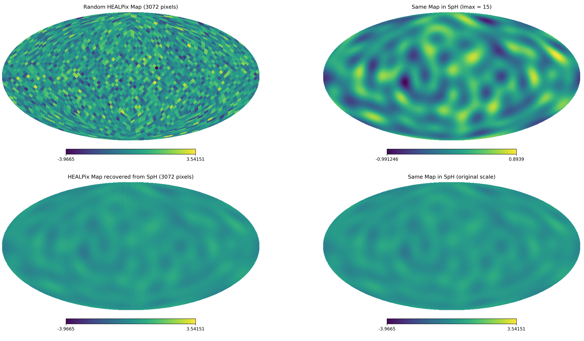
Furthermore, HEALPix offers ready-made tools to provide spherical harmonic transform of a pixel-space map and vice-versa, via Fast Fourier Transform (FFT) by taking advantage of isoLatitude pixelization. Hence a separate search for anisotropic SGWB in a spherical harmonic domain may become redundant. We have used here the healpy package, the Python implementation of HEALPix.
III.3 Posing mapmaking as a matrix multiplication
Taking advantage of the compression achieved by folding, PyStoch is explicitly calculating for all time segments and performing Eqs. (20,II.2) as a matrix multiplication for a fixed frequency . This provides much more efficiency compared to the usual practice of looping over time segments and computing each component in place. When using folded data for the sky map making, the segment times and data lengths are predictable. Every data-segment can have previously determined start times, as the segment division is now in sidereal times. This allows pre-calculation of the overlap reduction function. Hence it reduces computational time significantly compared to the usual method of calculating the overlap reduction function (ORF) on-the-go for all available segments. This approach makes it easy to perform the analysis for a network of detectors by calculating the dirty map and Fisher matrix () for all detector pairs in the network and adding them.
III.4 Efficient computation of overlap reduction function
Calculation and storage of ORF for a sidereal day with a segment duration of sec and a bin size of Hz requires almost GB of RAM for a resolution corresponding to . PyStoch alleviates this high RAM requirement issue by introducing seed matrices for the ORF, which can be used to compute the ORF in a fast manner, alleviating the demand for an unusually large amount of memory.
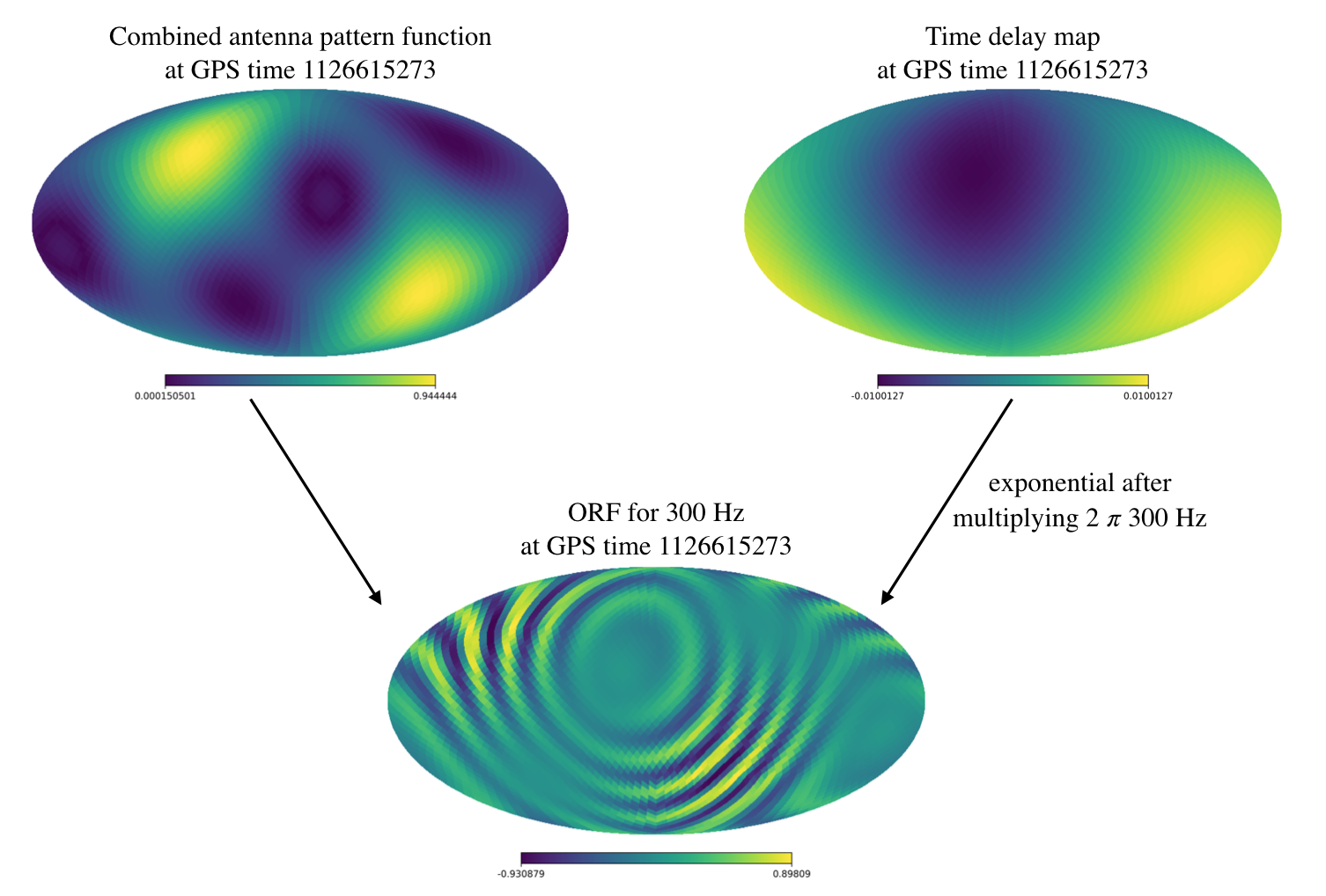
Let us consider the algebraic structure of ORF. It can be seen in Eq. (11) that the ORF depends on two components, the combined antenna pattern function, , and the time delay, , which have no frequency dependence and they are sky maps for a particular time segment. We call these two quantities the ORF seeds, which are easy to store in the RAM and can be used to calculate the ORF for each time segment and frequency bin. The combined antenna pattern function provides all possible combination of antenna pattern function corresponding to different detectors (in this demonstration we have used two), whereas from the phase factor expressed in the overlap reduction function one can find the time delay corresponding to each pixel. The quantity gives the time delay between two detectors in receiving a signal from a certain direction . The process is pictorially shown in Fig. 3.
III.5 Putting the pieces together
In this pipeline, our first step is to go through the folded data, produced by folding the entire data of LIGO’s observational run to a single sidereal day, and produce the combined antenna pattern function map for every time segment in the folded data. One can store this combined antenna pattern function maps as a matrix which has a dimension equal to the number of pixels times the number of time segments. Similarly, for the time delay maps one can calculate and store the delay between two detectors for different baselines as maps. This can be considered as calculating and storing the time delay for different time segments in a matrix having a dimension of the number of time segments times number of pixels. One can calculate and store these seed maps within no time as matrices using a small amount of RAM. This entire process of calculating and storing these quantities took only MB of RAM each. As a result, the pairs of seed maps corresponding to one sidereal day’s data with sec segment duration could be produced on a laptop in just seconds.
From these pairs of seed maps, by considering both the combined antenna pattern function map as well as the exponential of the time delay map, for each frequency one can calculate the overlap reduction function. This can also be stored as a matrix with dimension equal to the number of frequency segments times number of time segments.
Once we have the ORF, calculation of the dirty map is straightforward. The CSD and PSD are stored in two different channels in stochastic intermediate data (SID) or folded SID (FSID). The CSD and PSD are in the frequency domain, where the minimum and maximum frequencies and the frequency resolution of CSD and PSD determine how many frequency bins are there. We have to loop over all the frequency bins, and each iteration of the loop will produce one narrowband map for that frequency.
In each loop, the ORF is calculated from the ORF seeds for the particular frequency corresponding to that loop. Then the columns in CSD and PSD for that frequency are multiplied with the ORF. As per Eq. (28), the result is the narrowband map for that frequency. Looping over all the frequencies gives all the narrowband maps.
IV Implementation and Results
We have implemented the PyStoch code on LIGO’s first observational run (O1) data from the Hanford and Livingston detectors We have also used it for simulated data. Raw data from the detectors are down-sampled to 4 kHz and cross-correlated. Cross-correlation is done in the frequency domain for faster calculation. We then used the folding code to fold the data into one sidereal day. The folding code can take care of the overlap of the segments and data quality cuts, but the data we used already had it done during the cross-correlation. The output of folding is frames of sec segment duration which span a complete sidereal day.
PyStoch reads the parameters which are the same for all the frames (e.g., GPS start time, frequency cutoffs, segment durations, etc.) from the first frame. Then it reads the CSD and PSD from all other frames. We had our data in a spectrum where the lower and higher cutoff was 20 Hz and 1980 Hz respectively, and it had a resolution of 0.25 Hz. The HEALPix map resolution we choose corresponds to , which uses 3072 pixels for the entire sky (each pixel covers approximately 13 square degrees of the sky). The overlap reduction function had to be calculated for all the time segments. Each of the two sets of seed matrices was hence a matrix of dimension with each element a real number. The memory consumption of the seed matrices is 156MB. On a typical laptop (2.6 GHz processor, 4 CPU threads) it takes less than 20 seconds to calculate and save the seed matrices.
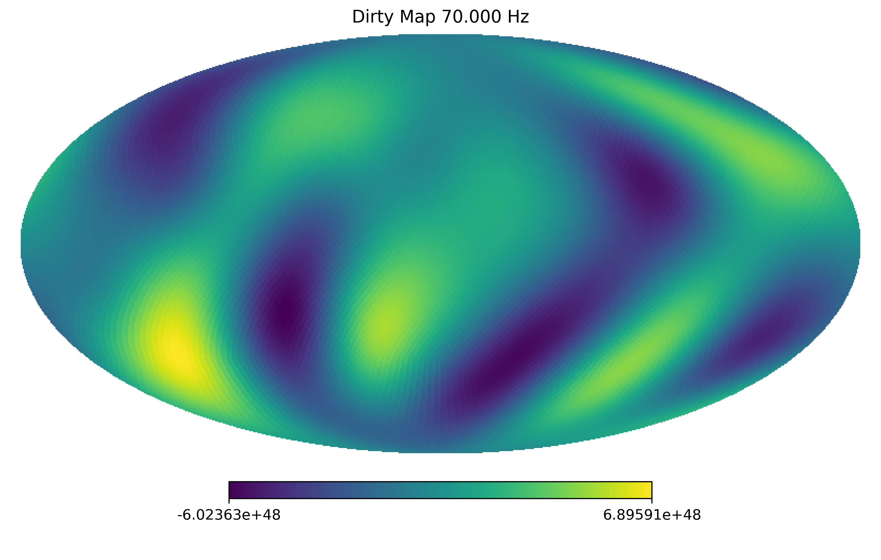
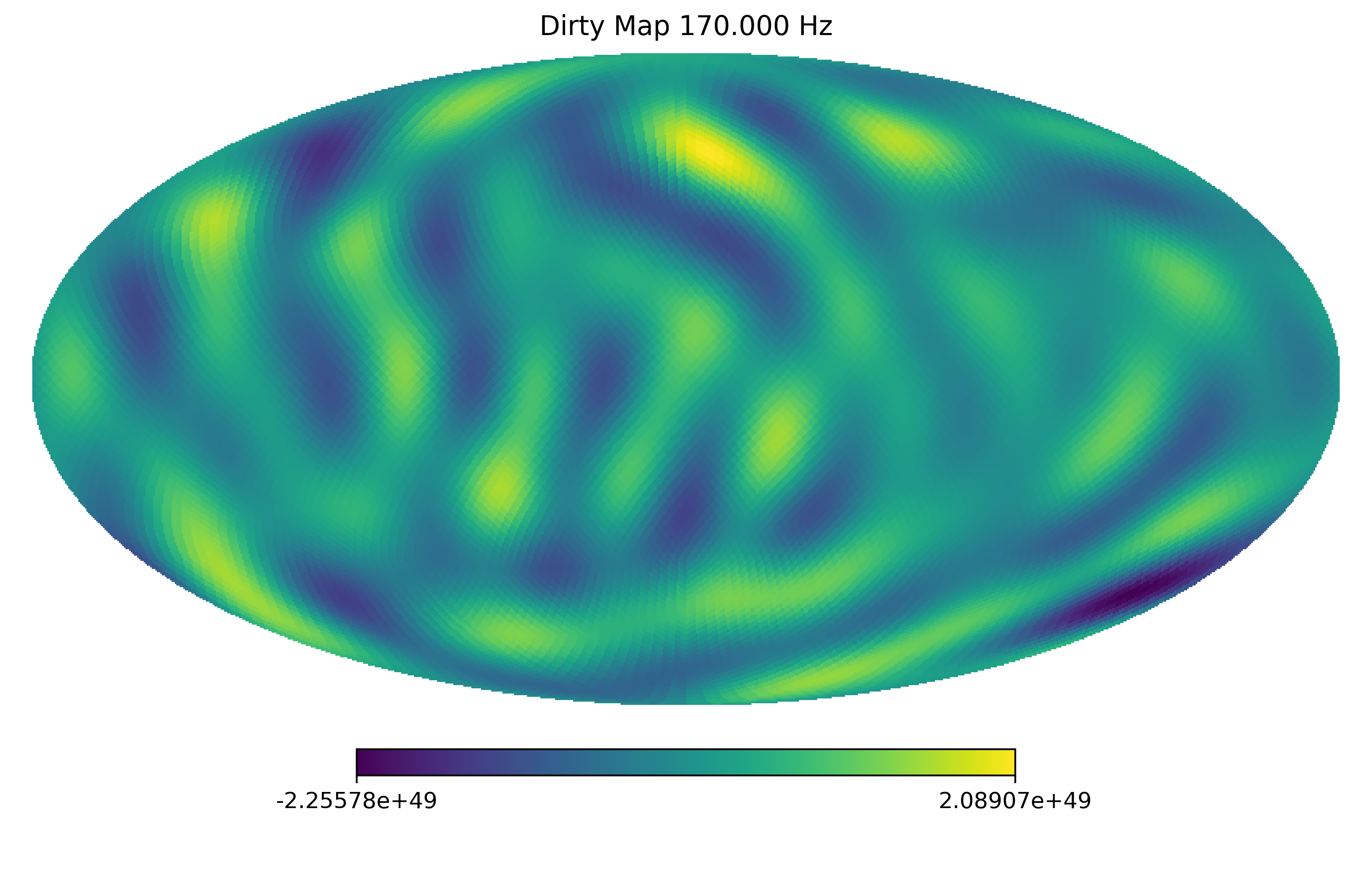
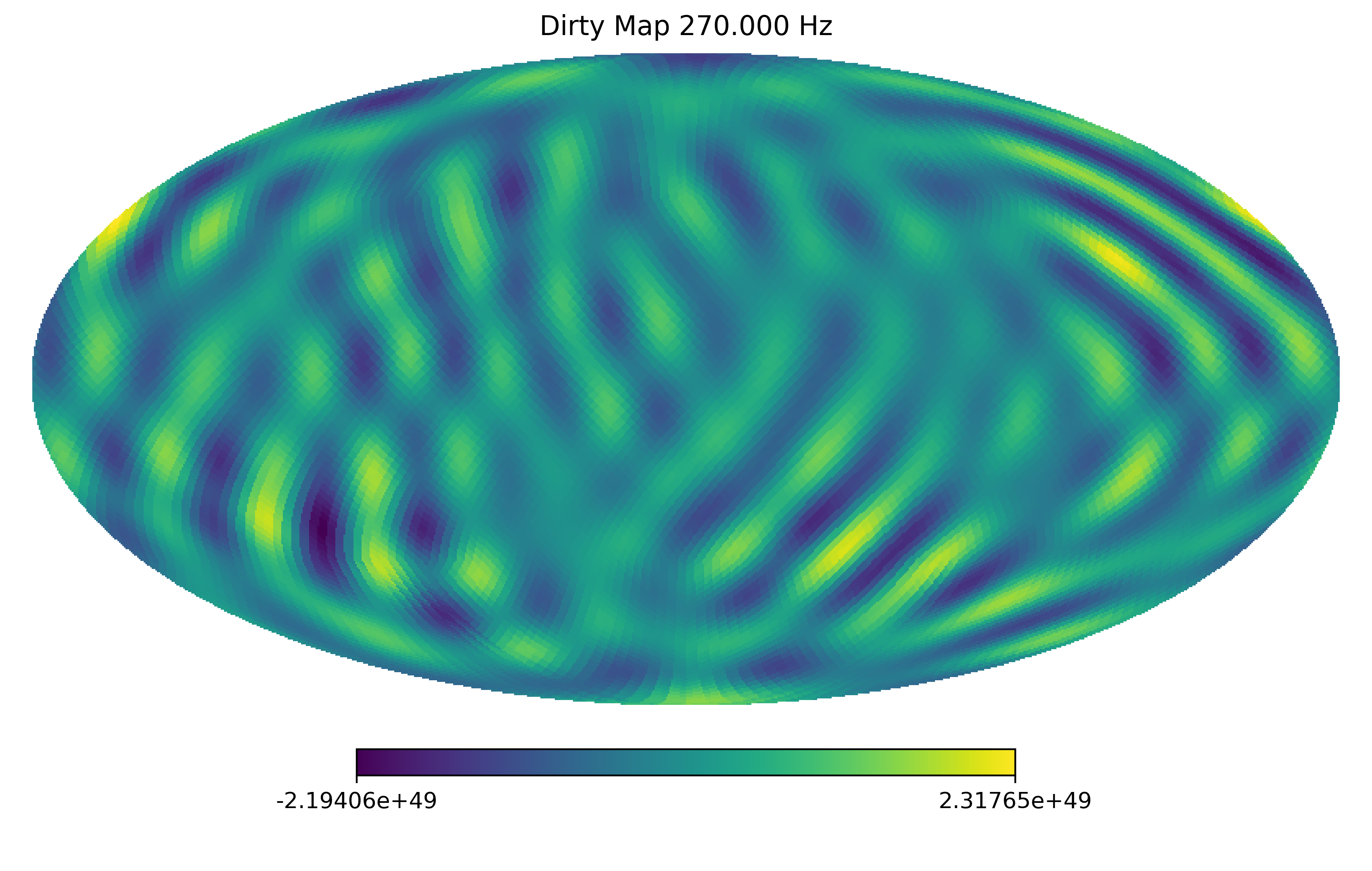
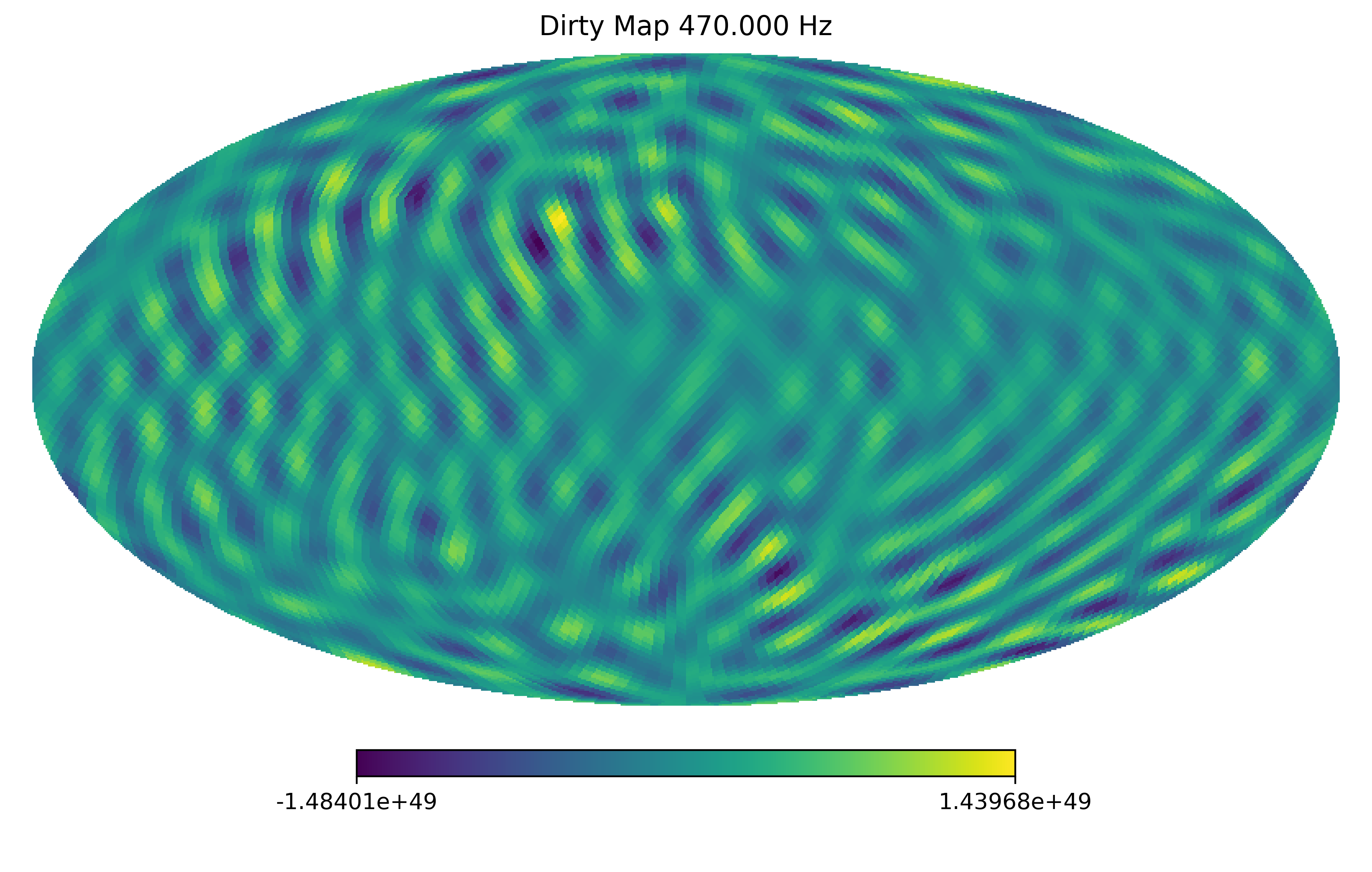
While calculating the narrowband maps, we restricted ourselves to an upper cutoff of 500 Hz, so we had 1920 frequency bins. Then we load the CSD () and PSD (). The appropriate frequency bins are taken for the calculations so the data (CSD and PSD) are matrices of . We now have to loop over frequencies. In each loop for a particular frequency, ORF is calculated using the ORF seed matrices. Then we take one column from the CSD and PSD matrices which is of the size . This corresponds to the data for that frequency and all time segments. When this data column is multiplied with the ORF, we get a matrix. This matrix is the narrowband map for that frequency. In Fig. 4, of the narrowband maps generated from simulated data are shown. This simulated data which we used is generated by adding a random phase factor to the O1 CSD for all frequency bins. This preserves the statistical properties of the data but renders the results unphysical.
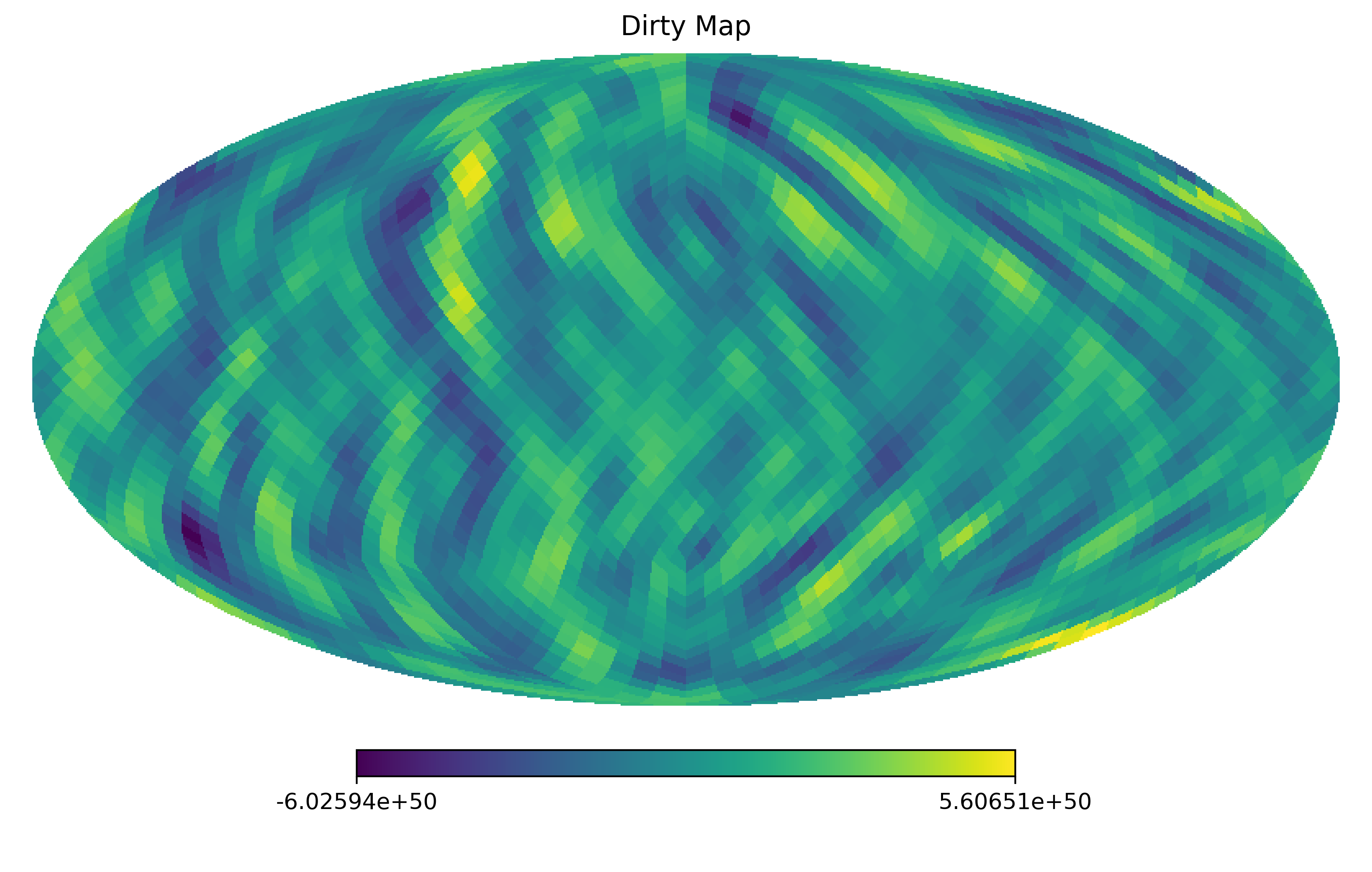
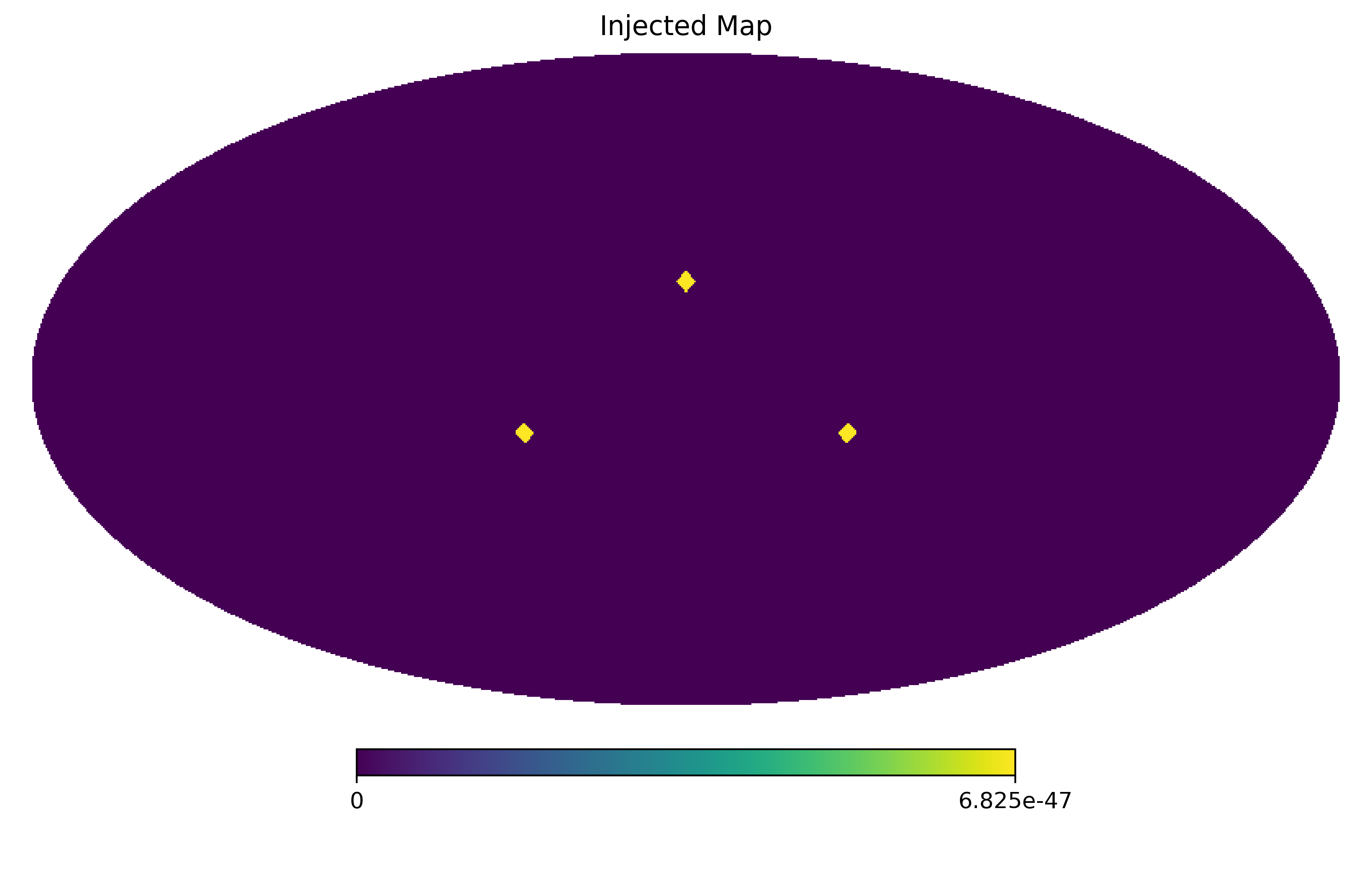
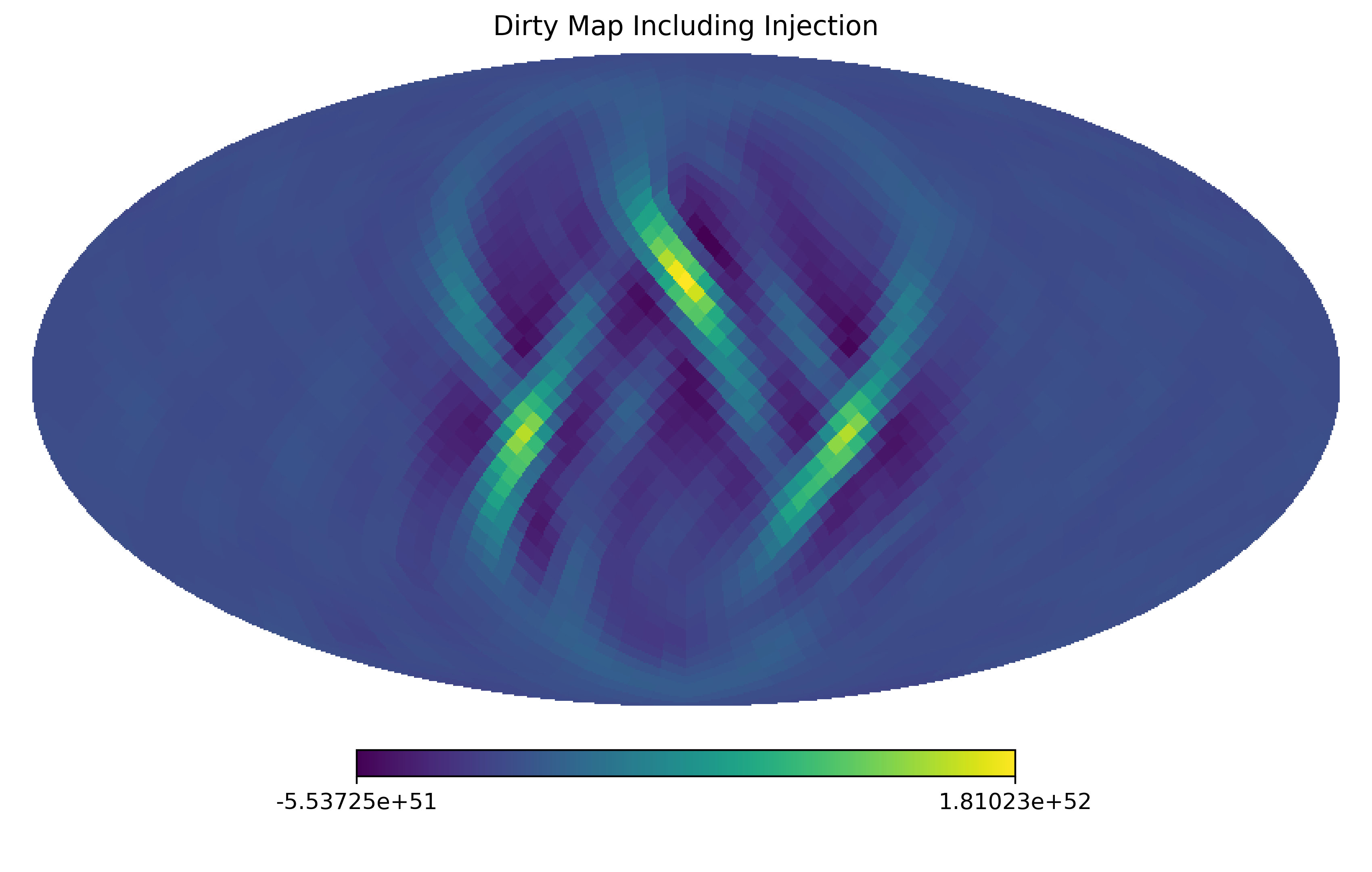
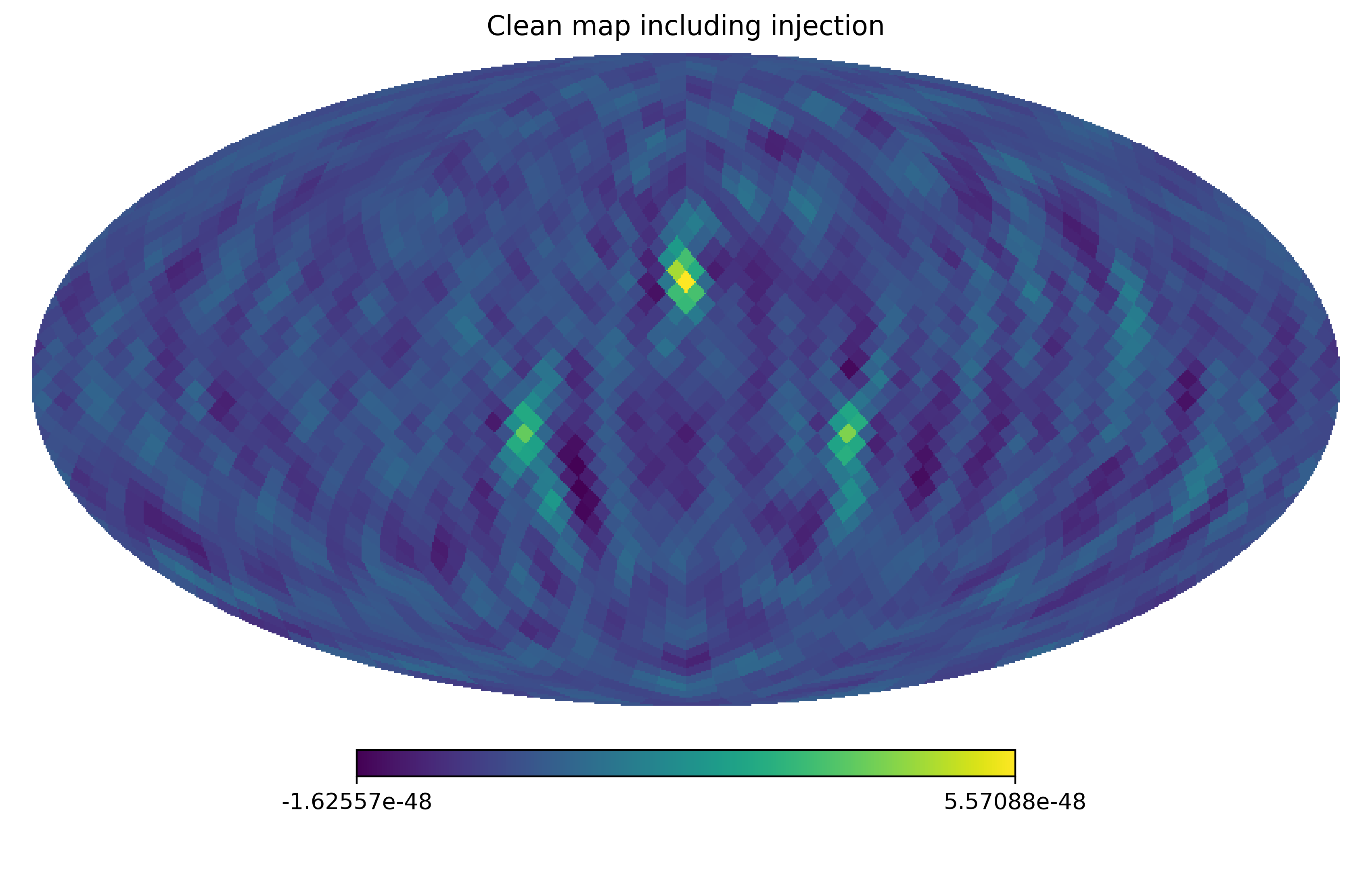
To further validate PyStoch, we tested the code with some injections. The injection sources we used were broadband point sources with a flat spectrum at three different points of the sky, the strengths were two orders higher than the noise PSD. We calculated the CSD for these injected sources and added them to the CSD data. After running the code, the injected sources were properly recovered. The results from applying this injection on simulated data are shown in Fig. 5. This figure also includes a map in the bottom right which is obtained by deconvolution of the dirty map with a Fisher matrix. This was a check to see if the source strength and location in the clean map match the injected map. In this case, the point sources in the clean map appears at the same location as the injected map, thus validating the deconvolution method. Moreover, the point sources in the clean map are more localized than in the dirty map.
V Conclusions
The primary advantage of PyStoch is the speed up and convenience. It makes the map calculation few hundred times faster333Tens of times faster on a single thread, hundred times faster when used with multi-threading.. Table 1 shows the scale of speed up by folding and PyStoch. It also gets rid of the requirement for storage to save intermediate results. With folding and PyStoch SGWB searches with LIGO data can be done on a laptop, in place of parallel computing on few hundred processors, which is very convenient.
| Conventional Pipeline | Folding Pipeline | Folding and PyStoch | |
|---|---|---|---|
| Intermediate Data | 450 GB | 1.5 GB | 1.5 GB |
| Processing Time | 10 CPU years | 10 CPU days | 40 CPU minutes |
| Intermediate Results | 800 TB | 2.5 TB | not required |
| Final Results | 500 MB | 500 MB | 500 MB |
Another advantage is that PyStoch produces results regarding narrowband maps. In the older pipeline one had to specify the expected SGWB spectrum before running the pipeline. But PyStoch does not require the spectrum. From Eq. (28), the set of narrowband maps, the spectrum-specific result can be produced using the following equation,
| (29) |
The above summation of narrowband maps can be done in one matrix multiplication. Also, PyStoch is a directed search for all directions in the sky, which means that if one wants to search a particular direction of the sky, e.g., Sco X-1 or Virgo cluster, it is straightforward. We only have to see which pixel(s) include the source and we can just add the pixels (since HEALPix pixels corresponds to the equal area in the sky one does not even have to worry about pixel weights). Similarly, PyStoch search results can be contracted into the result of isotropic search just by adding all the pixel values. All data quality cuts, removing bad frequencies (notch list) and correction for the windowing and the segment overlaps can be incorporated during or before running PyStoch.
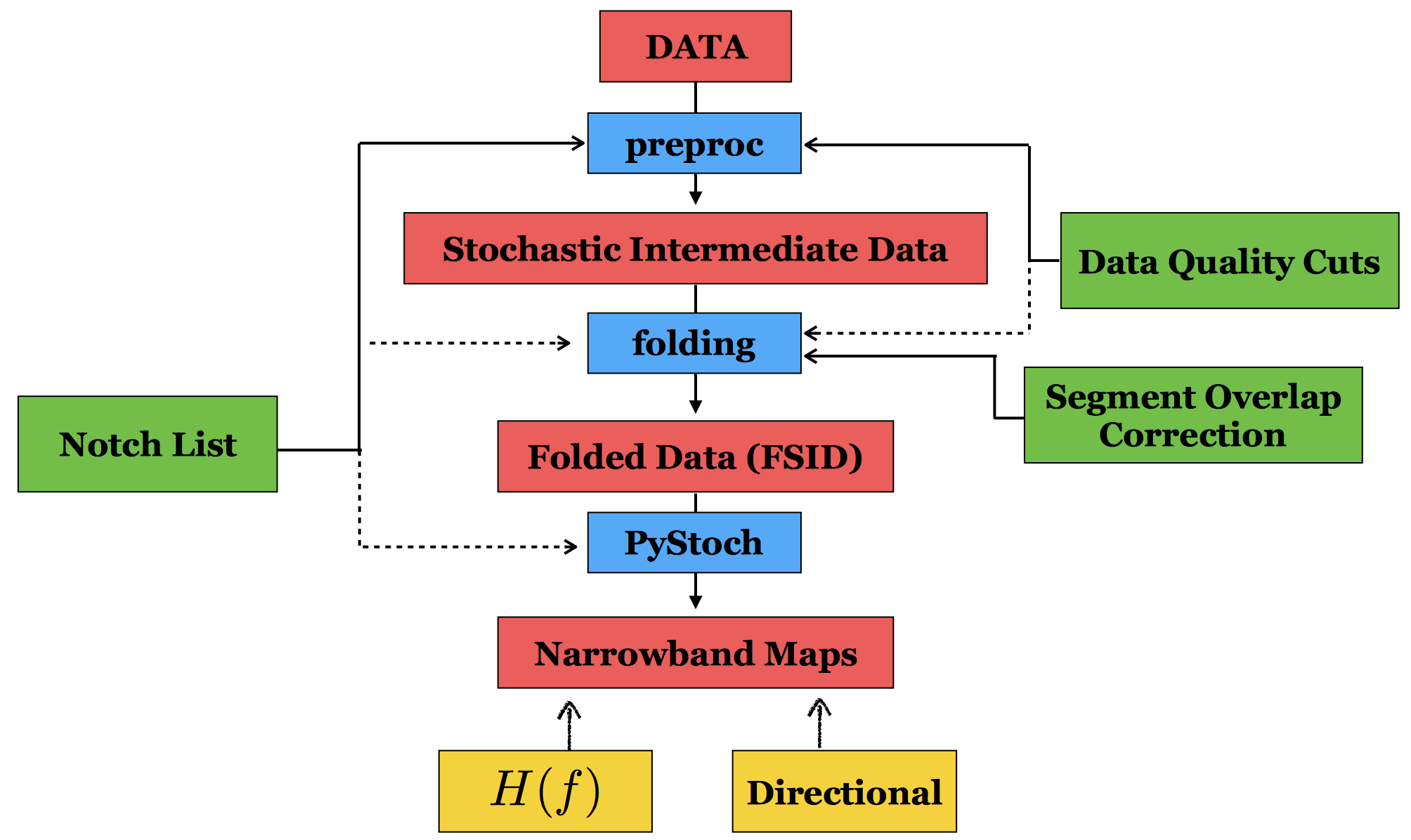
The enormous efficiency achieved by folding is further enormously amplified by PyStoch. Folding makes the analysis few hundred times faster, PyStoch also makes the analysis few ten times faster. So our new algorithm for stochastic analysis (Fig. 6) is about ten thousand times faster than the standard pipeline, and the results are more general and versatile. PyStoch automatically uses multi-threading when utilized by a multi-core CPU. This can make the SGWB search even faster. Also, this new pipeline eliminate the need for intermediate data storage. The results of PyStoch are more practical. In future, PyStoch will enable more in-depth searches and maps of SGWB.
PyStoch uses PyCBC routines to calculate the ORF. PyCBC has information about other detectors (aVIRGO, GEO600, KAGRA, etc. Acernese et al. (2015); Willke et al. (2002); Somiya (2012)) incorporated into it. This makes it very easy to tweak PyStoch for baselines other than the Livingston-Hanford baselines. We have tested it for many different baselines. As a toy model, let us consider the situation where VIRGO becomes as sensitive as AdvLIGO and when LIGO-India starts operating. In these scenarios, PyStoch can be easily used to map the SGWB using the global network of terrestrial detectors.
VI Acknowledgment
We thank the LIGO Scientific Collaboration for access to the data and gratefully acknowledge the support of the United States National Science Foundation (NSF) for the construction and operation of the LIGO Laboratory and Advanced LIGO as well as the Science and Technology Facilities Council (STFC) of the United Kingdom, and the Max-Planck-Society (MPS) for support of the construction of Advanced LIGO. Additional support for Advanced LIGO was provided by the Australian Research Council. We thank Dr. Andrew Matas and rest of the stochastic working group of LIGO for their help with the stochastic pipeline and their valuable comments. We acknowledge the use of IUCAA LDG cluster Sarathi for the computational/numerical work. This research benefited from a grant awarded to IUCAA by the Navajbai Ratan Tata Trust (NRTT). A. A. acknowledges the support of Council of Scientific and Industrial Research (CSIR), India. S. M. acknowledges support from the Department of Science & Technology (DST), India provided under the Swarna Jayanti Fellowships scheme.
References
- Abbott et al. (2016a) B. P. Abbott et al. (Virgo, LIGO Scientific), Phys. Rev. Lett. 116, 061102 (2016a), eprint 1602.03837.
- Abbott et al. (2016b) B. P. Abbott et al. (Virgo, LIGO Scientific), Phys. Rev. X6, 041015 (2016b), eprint 1606.04856.
- Abbott et al. (2017a) B. P. Abbott et al. (VIRGO, LIGO Scientific), Phys. Rev. Lett. 118, 221101 (2017a), eprint 1706.01812.
- Abbott et al. (2017b) B. P. Abbott et al. (Virgo, LIGO Scientific), Astrophys. J. 851, L35 (2017b), eprint 1711.05578.
- Abbott et al. (2017c) B. P. Abbott et al. (Virgo, LIGO Scientific), Phys. Rev. Lett. 119, 141101 (2017c), eprint 1709.09660.
- Abbott et al. (2017d) B. Abbott et al. (Virgo, LIGO Scientific), Phys. Rev. Lett. 119, 161101 (2017d), eprint 1710.05832.
- Collaboration et al. (2015) T. L. S. Collaboration, J. Aasi, B. P. Abbott, R. Abbott, T. Abbott, M. R. Abernathy, K. Ackley, C. Adams, T. Adams, P. Addesso, et al., Classical and Quantum Gravity 32, 074001 (2015).
- Acernese et al. (2015) F. Acernese et al. (VIRGO), Tech. Rep. 2 (2015), eprint 1408.3978.
- Affeldt et al. (2014) C. Affeldt et al., Class. Quant. Grav. 31, 224002 (2014).
- Ando and the TAMA collaboration (2002) M. Ando and the TAMA collaboration, Classical and Quantum Gravity 19, 1409 (2002).
- Somiya (2012) K. Somiya (KAGRA), Class. Quant. Grav. 29, 124007 (2012), eprint 1111.7185.
- Hobbs et al. (2010) G. Hobbs et al., Classical and Quantum Gravity 27, 084013 (2010), eprint 0911.5206.
- Amaro-Seoane et al. (2013) P. Amaro-Seoane, S. Aoudia, S. Babak, P. Binétruy, E. Berti, A. Bohé, C. Caprini, M. Colpi, N. J. Cornish, K. Danzmann, et al., GW Notes, Vol. 6, p. 4-110 6, 4 (2013), eprint 1201.3621.
- Seiji Kawamura et al. (2011) Seiji Kawamura et al., Classical and Quantum Gravity 28, 094011 (2011).
- Harry et al. (2006) G. M. Harry, P. Fritschel, D. A. Shaddock, W. Folkner, and E. S. Phinney, Classical and Quantum Gravity 23, 4887 (2006).
- Einstein (1918) A. Einstein, Sitzungsberichte der Königlich Preussischen Akademie der Wissenschaften p. 154 (1918).
- Misner et al. (1973) C. W. Misner, K. S. Thorne, and J. A. Wheeler, Gravitation (Freeman, New York, USA, 1973).
- Thorne (1987) K. S. Thorne, in 300 Years of Gravitation (Cambridge University Press, Cambridge, UK, 1987).
- Regimbau and Mandic (2008) T. Regimbau and V. Mandic, Classical and Quantum Gravity 25, 184018 (2008), eprint 0806.2794.
- Coward and Regimbau (2006) D. Coward and T. Regimbau, New Astron.Rev. 50, 461 (2006), eprint astro-ph/0607043.
- Allen (1996) B. Allen (1996), eprint gr-qc/9604033.
- Grishchuk (2001) L. P. Grishchuk, in Gyros, Clocks, Interferometers: Testing Relativistic Gravity in Space, edited by C. Lämmerzahl, C. W. F. Everitt, and F. W. Hehl (2001), vol. 562 of Lecture Notes in Physics, Berlin Springer Verlag, p. 167, eprint gr-qc/0002035.
- Turner (1997) M. S. Turner, Phys. Rev. D 55, 435 (1997), eprint astro-ph/9607066.
- Dhurandhar et al. (2011) S. Dhurandhar, H. Tagoshi, Y. Okada, N. Kanda, and H. Takahashi, Phys. Rev. D 84, 083007 (2011).
- Mazumder et al. (2014) N. Mazumder, S. Mitra, and S. Dhurandhar, Phys. Rev. D 89, 084076 (2014), eprint 1401.5898.
- Geller et al. (2018) M. Geller, A. Hook, R. Sundrum, and Y. Tsai, ArXiv e-prints (2018), eprint 1803.10780.
- Jenkins and Sakellariadou (2018) A. Jenkins and M. Sakellariadou, ArXiv e-prints (2018), eprint 1802.06046.
- Allen and Ottewill (1997) B. Allen and A. C. Ottewill, Phys. Rev. D 56, 545 (1997), eprint gr-qc/9607068.
- Allen (1988) B. Allen, Phys. Rev. D 37, 2078 (1988).
- Sesana et al. (2008) A. Sesana, A. Vecchio, and C. N. Colacino, Mon. Not. Roy. Astron. Soc. 390, 192 (2008), eprint 0804.4476.
- Romano and Cornish (2017) J. D. Romano and N. J. Cornish, Living Rev. Rel. 20, 2 (2017), eprint 1608.06889.
- Michelson (1987) P. F. Michelson, Mon. Not. Roy. Astron. Soc. 227, 933 (1987).
- Christensen (1992) N. Christensen, Phys. Rev. D46, 5250 (1992).
- Flanagan (1993) E. E. Flanagan, Phys. Rev. D48, 2389 (1993).
- Allen and Romano (1999) B. Allen and J. D. Romano, Phys. Rev. D59, 102001 (1999), eprint gr-qc/9710117.
- Cornish (2001) N. J. Cornish, Phys. Rev. D65, 022004 (2001), eprint gr-qc/0106058.
- Lazzarini and Weiss (2004) A. Lazzarini and R. Weiss, Internal working note LIGO-T040140-00-Z, Laser Interferometer Gravitational Wave Observatory (LIGO) (2004).
- Ballmer (2006) S. W. Ballmer, Class. Quant. Grav. 23, S179 (2006), eprint gr-qc/0510096.
- Mitra et al. (2008) S. Mitra, S. Dhurandhar, T. Souradeep, A. Lazzarini, V. Mandic, et al., Phys.Rev. D77, 042002 (2008), eprint 0708.2728.
- Thompson et al. (2001) A. R. Thompson, J. M. Moran, and G. W. Swenson, Jr., Interferometry and Synthesis in Radio Astronomy, 2nd Edition (Wiley-VCH, 2001).
- Ryle and Hewish (1960) M. Ryle and A. Hewish, Mon. Not. Roy. Astron. Soc. 120, 220 (1960).
- Thrane et al. (2009) E. Thrane, S. Ballmer, J. D. Romano, S. Mitra, D. Talukder, S. Bose, and V. Mandic, Phys. Rev. D80, 122002 (2009), eprint 0910.0858.
- Aasi et al. (2014) J. Aasi et al., Physical Review Letters 113, 231101 (2014), eprint 1406.4556.
- Abbott et al. (2009) B. P. Abbott et al., Nature 460, 990 (2009), eprint arXiv:0910.5772.
- Abbott et al. (2007a) B. Abbott et al., Phys. Rev. D 76, 082003 (2007a), eprint astro-ph/0703234.
- Abadie et al. (2011) J. Abadie et al., Phys. Rev. Lett. 107, 271102 (2011), eprint 1109.1809.
- Abbott et al. (2007b) B. Abbott et al., Phys. Rev. D 76, 022001 (2007b), eprint gr-qc/0703068.
- Mingarelli et al. (2013) C. M. F. Mingarelli, T. Sidery, I. Mandel, and A. Vecchio, Phys. Rev. D88, 062005 (2013), eprint 1306.5394.
- Taylor and Gair (2013) S. R. Taylor and J. R. Gair, Phys. Rev. D88, 084001 (2013), eprint 1306.5395.
- Taylor et al. (2015) S. Taylor, C. Mingarelli, J. Gair, A. Sesana, G. Theureau, S. Babak, C. Bassa, P. Brem, M. Burgay, R. Caballero, et al., Phys. Rev. Lett. 115, 041101 (2015), eprint 1506.08817.
- Gair et al. (2015) J. R. Gair, J. D. Romano, and S. R. Taylor, Phys. Rev. D92, 102003 (2015), eprint 1506.08668.
- Ain et al. (2015) A. Ain, P. Dalvi, and S. Mitra, Phys. Rev. D92, 022003 (2015), eprint 1504.01714.
- Thrane et al. (2015) E. Thrane, S. Mitra, N. Christensen, V. Mandic, and A. Ain, Phys. Rev. D 91, 124012 (2015).
- Gorski et al. (2005) K. M. Gorski, E. Hivon, A. J. Banday, B. D. Wandelt, F. K. Hansen, M. Reinecke, and M. Bartelman, Astrophys. J. 622, 759 (2005), eprint astro-ph/0409513.
- Abbott et al. (2017e) B. P. Abbott et al. (Virgo, LIGO Scientific), Phys. Rev. Lett. 118, 121102 (2017e), eprint 1612.02030.
- Finn et al. (2009) L. S. Finn, S. L. Larson, and J. D. Romano, Phys. Rev. D79, 062003 (2009), eprint 0811.3582.
- Abbott et al. (2017f) B. P. Abbott et al. (Virgo, LIGO Scientific), Phys. Rev. Lett. 118, 121101 (2017f), [Erratum: Phys. Rev. Lett.119,no.2,029901(2017)], eprint 1612.02029.
- Lazzarini and Romano (2004) A. Lazzarini and J. Romano, Internal working note LIGO-T040089-00-Z, Laser Interferometer Gravitational Wave Observatory (LIGO) (2004).
- Dal Canton et al. (2014) T. Dal Canton et al., Phys. Rev. D90, 082004 (2014), eprint 1405.6731.
- Usman et al. (2016) S. A. Usman et al., Class. Quant. Grav. 33, 215004 (2016), eprint 1508.02357.
- Willke et al. (2002) B. Willke et al., Class. Quant. Grav. 19, 1377 (2002).