Stochastic PDE Limit of the Six Vertex Model

Abstract.

We study the stochastic six vertex model and prove that under weak asymmetry scaling (i.e., when the parameter $\Delta\to 1^{+}$ so as to zoom into the ferroelectric/disordered phase critical point) its height function fluctuations converge to the solution to the Kardar–Parisi–Zhang (KPZ) equation. We also prove that the one-dimensional family of stochastic Gibbs states for the symmetric six vertex model converge under the same scaling to the stationary solution to the stochastic Burgers equation.

Our proofs rely upon the Markov (self) duality of our model. The starting point is an exact microscopic Hopf–Cole transform for the stochastic six vertex model which follows from the model’s known one-particle Markov self-duality. Given this transform, the crucial step is to establish self-averaging for specific quadratic function of the transformed height function. We use the model’s two-particle self-duality to produce explicit expressions (as Bethe ansatz contour integrals) for conditional expectations from which we extract time-decorrelation and hence self-averaging in time. The crux of our Markov duality method is that the entire convergence result reduces to precise estimates on the one-particle and two-particle transition probabilities. Previous to our work, Markov dualities had only been used to prove convergence of particle systems to linear Gaussian SPDEs (e.g. the stochastic heat equation with additive noise).

1. Introduction

The Six Vertex (6V) model and the KPZ equation are widely studied models in equilibrium and non-equilibrium statistical mechanics. In this paper we demonstrate how a certain scaling limit of the former model converges to the later equation. This limit comes from scaling into the critical point dividing the ferroelectric and disordered phases of the model. Our results apply for both the stochastic and symmetric 6V models (Theorems 1.1 and 1.6 respectively). The technical core of this paper is the Markov duality method: One-particle duality allows us to perform a microscopic Hopf–Cole transform of the model’s height function process into a discrete stochastic heat equation, and prove tightness of that resulting equation; and two-particle duality controls the quadratic variation of the martingale part and proves precise self-averaging in time.

The structure of this introduction is as follows: Section 1.1 introduces the stochastic 6V model and records our first main result, it convergence to the KPZ equation (Theorem 1.1). Section 1.2 introduces the symmetric 6V model and records our second main result, the convergence of the one-parameter family of stochastic Gibbs states to the stationary solution to the stochastic Burgers equation (Theorem 1.6). This section also describes the model with external fields and how the stochastic Gibbs states arise in the (conjectural) phase diagram for the model’s Gibbs states. Section 1.3 recalls how the KPZ equation arises as a scaling limit for ASEP (a well studied continuous time limit of the stochastic 6V model). The purpose of this is to highlight (in the simplest case possible) the key technical challenge in proving such results—self average of the quadratic variation. Section 1.4 briefly introduces our Markov duality method in the context of ASEP and provides some historical context for it. This approach is developed fully for the stochastic 6V model in the main body of the paper. Section 1.5 provides a brief review of related literature studying the symmetric and stochastic 6V models, KPZ equation, and Markov dualities.

1.1. KPZ equation as a limit of the stochastic six vertex model

The stochastic 6V model is a discrete time interacting particle system introduced in 1992 by Gwa and Spohn [GS92]. The model depends on two parameters $b_{1},b_{2}\in(0,1)$ which are used to define (positive) weights on six type of vertices—see the top row of Figure 1. Treating the solid lines entering a vertex from below or the left as inputs and those exits above or to the right as outputs, these vertex are conservative (i.e., the number of input lines equals the number of output lines) and stochastic (i.e., for fixed inputs, the sum of weights over outputs is always 1, and the individual weights are non-negative). Given a down-right path in $\mathbb{Z}^{2}$ and a specification of boundary condition inputs along the path, the stochastic 6V model is a measure on the vertices to the up and right of the path, or equivalently a measure on the collection of solid lines which leave the boundary inputs and continue in the up and right directions. The measure is defined recursively: starting with vertices with inputs given, the outputs are randomly chosen amongst all possible outputs with probabilities given by the associated vertex weights. The left-side of Figure 2 illustrates when the boundary condition inputs are specified on the coordinate axes for the first quadrant. See Section 2.1 for a more precise definition of the model (including a bi-infinite version) and Section 1.5.2 for a brief review of related literature.

Non-crossing paths
Stochastic weights	$1$	$1$	$b_{1}$	$b_{2}$	$1-b_{1}$	$1-b_{2}$
Symmetric weights	$a$	$a$	$b$	$b$	$c$	$c$
Asymmetric weights	$e^{-H-V}a$	$e^{H+V}a$	$e^{-H+V}b$	$e^{H-V}b$	$c$	$c$

Figure 1. Six vertices with their stochastic, symmetric and asymmetric weights.

If the boundary condition inputs are specified entirely on the horizontal axis, it is natural to think of vertical solid lines as particles evolving in time (as measured by the $y$-coordinate) via the following Markovian update. Start with left-most particle. With probability $b_{1}$ it stays put, and with $1-b_{1}$ it moves one to the right. The particle continues to move right with probability $b_{2}$ per step until it either stops, or it hits the next particle. When no collision happens, repeat these rules for the next particle to the right. If a collision occurs, the moving particle stops at that site and the next particle starts moving to the right with probability $1$, and continues to move with probability $b_{2}$ (as usual). See Section 1.5.2 for a discussion of some limit of the stochastic 6V model.

Figure 2. Left: Particle trajectories for the stochastic 6V model with boundary condition inputs along the coordinate axes. Right: Periodic boundary conditions.

Define the height function $N(t,x)$ for the stochastic 6V model to be equal to the net number of particles which have moved across the time-space line between $(0,0)$ and $(t,x)$ (i.e., summing $1$ for each left-to-right move and $-1$ for each right-to-left move—see Figure 3). For a precise definition as well as a construction of $N(t,x)$ for bi-infinite configurations, see Section 2.1. Given such $N(t,x)$, we first linearly interpolate in $x\in\mathbb{Z}$ and then linearly interpolate in $t\in\mathbb{Z}_{\geq 0}$ to make $N(t,x)\in C([0,\infty),C(\mathbb{R}))$. Hereafter, we endow the space $C(\mathbb{R})$ and $C([0,\infty),C(\mathbb{R}))$ the topology of uniform convergence over compact subsets, and write $\Rightarrow$ for the weak convergence of probability laws.

Figure 3. The stochastic 6V particle trajectories and associated height functions. Here we assume a left-most particle and label the first five particles $x_{1},\ldots,x_{5}$. The lines represent their temporal trajectories. The dark grey numbers represent the height function $N(t,y)$ for different regions. The height function changes value when crossing particle trajectories (increasing as one crosses from left to right).

Our main result for the stochastic 6V model states that, under weak asymmetry scaling where $b_{1}\in(0,1)$ is fixed and $\tau=b_{2}/b_{1}=e^{-\sqrt{\varepsilon}}\to 1$, an analog of (1.26) holds for $N(t,x)$. To setup notations, we fix any density $\rho\in(0,1)$ hereafter, and let

$$\lambda =\frac{1-b_{2}\tau^{-\rho}}{b_{1}-(b_{1}+b_{2}-1)\tau^{-\rho}}=\frac{1-b_{1}\tau^{1-\rho}}{b_{1}-(b_{1}+b_{1}\tau-1)\tau^{-\rho}},$$ (1.1)

$$\mu =\frac{\tau^{-\rho}(1-b_{1})(1-b_{2})}{(b_{1}-(b_{1}+b_{2}-1)\tau^{-\rho})(1-b_{2}\tau^{-\rho})}=\frac{\tau^{-\rho}(1-b_{1})(1-b_{1}\tau)}{(b_{1}-(b_{1}+b_{1}\tau-1)\tau^{-\rho})(1-b_{1}\tau^{1-\rho})}.$$ (1.2)

The reason of choosing these values of the parameters $\lambda,\mu$ will be clear in Section 4.1. Specifically, under the weak asymmetry scaling where $b_{1}\in(0,1)$ fixed and $\tau=\tau_{\varepsilon}=b_{2}/b_{1}:=e^{-\sqrt{\varepsilon}}$, we have $\lambda=\lambda_{\varepsilon}$ and $\mu=\mu_{\varepsilon}$, which, up to first order in $\sqrt{\varepsilon}$, read

$$\lambda_{\varepsilon} =1-\rho\sqrt{\varepsilon}+\mathcal{O}(\varepsilon),$$ (1.3)

$$\mu_{\varepsilon} =1+\tfrac{b_{1}-2b_{1}\rho}{b_{1}-1}\sqrt{\varepsilon}+\mathcal{O}(\varepsilon).$$ (1.4)

We adopt standard notation $\mathcal{O}(a)$ to denote a generic quantity such that $\sup_{0<a<1}|\mathcal{O}(a)|a^{-1}<\infty$. Recall the KPZ equation (see Section 4.2 for its definition; Sections 1.3 and 1.5.3 a literature review).

$$\partial_{t}\mathcal{H}(t,x)=\frac{\nu_{*}}{2}\partial_{x}^{2}\mathcal{H}(t,x)-\frac{\kappa_{*}}{2}\big{(}\partial_{x}\mathcal{H}(t,x)\big{)}^{2}+\sqrt{D_{*}}\xi(t,x),$$ (1.5)

with coefficients

$$\nu_{*}:=\frac{2b_{1}}{1-b_{1}},\quad\kappa_{*}:=\frac{2b_{1}}{1-b_{1}},\quad D_{*}:=\frac{2b_{1}\rho(1-\rho)}{1-b_{1}}.$$ (1.6)

Theorem 1.1.

Consider the stochastic 6V model, with parameter $b_{1}>b_{2}\in(0,1)$.

1. (Near stationary initial conditions) Fix a density $\rho\in(0,1)$. With $\varepsilon\downarrow 0$ denoting a scaling parameter, we start the stochastic 6V model from a sequence of initial conditions $\{N_{\varepsilon}(0,x)\}_{\varepsilon>0}$, and let $N_{\varepsilon}(t,x)$ denote the resulting height function. Assume that $\{N_{\varepsilon}(0,x)\}_{\varepsilon>0}$ is near stationary with density $\rho$ (Definition 4.4), and that for some $C(\mathbb{R})$-valued process $\mathcal{H}^{\text{ic}}(x)$,

   $$\sqrt{\varepsilon}\big{(}N_{\varepsilon}(0,\varepsilon^{-1}x)-\rho\varepsilon^{-1}x\big{)}\Longrightarrow\mathcal{H}^{\text{ic}}(x),\quad\text{ in }C(\mathbb{R}).$$ (1.7)

   Then, under the weak asymmetry scaling where $b_{1}\in(0,1)$ is fixed, $\tau=\tau_{\varepsilon}=b_{2}/b_{1}:=e^{-\sqrt{\varepsilon}}$, and $\lambda$ and $\mu$ depend on $\varepsilon$ as in (1.3) and (1.4), we have

   $$\sqrt{\varepsilon}\Big{(}N_{\varepsilon}\big{(}\varepsilon^{-2}t,\varepsilon^{-1}x+\mu_{\varepsilon}\varepsilon^{-2}t\big{)}-\rho(\varepsilon^{-1}x+\mu_{\varepsilon}\varepsilon^{-2}t)\Big{)}-\varepsilon^{-2}t\log\lambda_{\varepsilon}\Longrightarrow \mathcal{H}(t,x),$$ (1.8)

   $$\text{in }C([0,\infty),C(\mathbb{R})),$$

   where $\mathcal{H}(t,x)$ is the Hopf–Cole solution (defined in Section 4.2) of the KPZ equation (1.5) with initial condition $\mathcal{H}^{\text{ic}}(x)$.

2. (Step initial condition) Start the stochastic 6V model from the step initial condition $N(0,x)=(x)_{+}:=\max(0,x)$, and let $N_{\varepsilon}(t,x)$ denote the resulting height function. Fix $\rho\in(0,1)$. Under the weak asymmetry scaling where $b_{1}\in(0,1)$ is fixed, $\tau=\tau_{\varepsilon}=b_{2}/b_{1}:=e^{-\sqrt{\varepsilon}}$, and $\lambda$ and $\mu$ depend on $\varepsilon$ as in (1.3) and (1.4), we have

   $$\sqrt{\varepsilon}\Big{(}N_{\varepsilon}\big{(}\varepsilon^{-2}t,\varepsilon^{-1}x+\mu_{\varepsilon}\varepsilon^{-2}t\big{)}-\rho(\varepsilon^{-1}x+\mu_{\varepsilon}\varepsilon^{-2}t)\Big{)}-\varepsilon^{-2}t\log\lambda_{\varepsilon} -\log\tfrac{\rho(1-\rho)}{\sqrt{\varepsilon}}\Longrightarrow\mathcal{H}(t,x),$$

   $$\text{in }C((0,\infty),C(\mathbb{R})),$$

   where $\mathcal{H}(t,x)$ is the Hopf–Cole solution of the KPZ equation (1.5) with narrow wedge initial condition (see Section 4.2).

Remark 1.2.

It is worth remarking on the freedom to choose arbitrary $\rho\in(0,1)$ in the theorem. For the near stationary initial conditions, $\rho$ controls the density of particles (or vertical lines) as well as the characteristic velocity around which we focus. For step initial data, $\rho$ determines a velocity within the rarefaction fan (and gives the density around that velocity). Previous KPZ equation limit results for ASEP where limited to $\rho=1/2$ since the arguments become more complicated in a moving frame or with a disproportionate number of particles to holes.

Remark 1.3.

[CT17] proves KPZ equation convergence for a portion of the class of higher spin stochastic vertex models [CP16]. Those models fall into two types – those with spin $I,J\in\mathbb{Z}_{\geq 1}$ in which the number of particles or arrows per edge is bounded by $I$ or $J$ (depending on the edge’s orientation) and those with non-integer spin in which there may be an infinite number of particles or arrows per edge. [CT17] analyzed this second class, specifically under scaling in which the expected number of particles per site diverges with $\varepsilon$. This simplifies analysis quite dramatically since [CT17] is able to Taylor expand the quadratic martingale in the density yielding an analysis which completely avoids the key complexity which we encounter here. The stochastic 6V model comes from taking $I=J=1$ and hence the number of particles per site is either 0 or 1. Though we do not address the general $I,J\in\mathbb{Z}_{\geq 1}$ class herein, we expect our Markov duality method is applicable there.

Remark 1.4.

Plugging the expansions (1.3) and (1.4) for $\lambda_{\varepsilon}$ and $\mu_{\varepsilon}$ into (1.8), one can see that the two terms of vertical shifting of height function, namely $-\sqrt{\varepsilon}\rho(\mu_{\varepsilon}\varepsilon^{-2}t)$ and $-\varepsilon^{-2}t\log\lambda_{\varepsilon}$, are both of order $\mathcal{O}(\varepsilon^{-\frac{3}{2}})$; but their order $\mathcal{O}(\varepsilon^{-\frac{3}{2}})$ parts cancel out. Therefore (1.8) states that the rescaled and tilted height function subtracting $\mathcal{O}(\varepsilon^{-1})t$ converges to the solution to KPZ equation.

Proof sketch. Proposition 4.1 provides an exact microscopic Hopf–Cole transform through which the stochastic 6V model height process is relates to a microscopic Stochastic Heat Equation (SHE). This transformation is readily seen as a consequence of the (one-particle) Markov self-duality given in Corollary 3.4. Theorem 1.1* proves convergence of this microscopic SHE to the continuum SHE. When translated back into the stochastic 6V model height function, this implies Theorem 1.1.

The proof of Theorem 1.1* boils down to showing tightness and identifying the limiting linear and quadratic martingale problem. The first two items follow in a standard manner from moment bounds provided by Proposition 5.4. Controlling the quadratic variation is the hard part. Proposition 5.6 does this by proving a form of self-averaging for the quadratic variation (which itself is a quadratic in the solution to the microscopic SHE). The proof of the self-average relies upon the two-particle duality through Proposition 4.3. That duality reduces the calculation of conditional expectations to computations involving the transition probability for a two-particle version of the stochastic 6V model. Such transition formulas can be written explicitly using Bethe ansatz—see Proposition 3.5 or the formula in (4.22). Proposition 6.1 contains very precise estimates on the two-point transition probabilities which are proved via involved steepest descent analysis on the double-contour integral formulas encoding these probabilities.

In Sections 1.3 and 1.4 (and Appendix A) we explain how these ideas work in the simpler the context of ASEP. For ASEP, there are other methods which can be used to prove self-averaging. Presently, our Markov duality method is the only approach which works for the 6V model.

1.2. Stochastic Burgers equation as a limit of symmetric six vertex model

The symmetric 6V model is a foundational model in 2D equilibrium statistical mechanics. It is defined with respect to a pre-imposed a choice of boundary condition on a compact domain in $\mathbb{Z}^{2}$, e.g. periodic boundary condition on a rectangular domain as in Figure 2. Then, one chooses an assignment of vertices inside the domain which fit together (i.e. output lines match input lines from vertices to the right or above) with probability proportional to the product of vertex weights. These weights are specified by $a,b,c>0$ (in fact, by scaling only two of these matter) as in Figure 1 and the model is called symmetric since reflecting the vertices over the diagonal does not change their weight. To go from such a product of weights to a probability requires dividing by a normalizing constant (also called a partition function) which is the sum over all configurations of the product of weights. The need to normalize was not present in the case of stochastic weights as it equals 1 there.

1.2.1. Conjectural phase diagram for symmetric six vertex model Gibbs states

How does the symmetric 6V model behave as the mesh size goes to zero? Is there a limit shape? How does the height function fluctuate around it? How much do boundary conditions or external fields effect these limits? These questions are intertwined with understanding the extremal, translation invariant, ergodic infinite volume Gibbs states (or simply Gibbs states for short) and their associated free energies. These can be thought of as distributions on configurations of vertices on $\mathbb{Z}^{2}$ which satisfy the symmetric 6V Gibbs property—the marginal distribution restricted to any compact subdomain, given the state of the boundary vertices, is given by the above symmetric 6V model probability prescription (i.e., product over weights of vertices normalized to be a probability distribution).

While much has been conjectured about the symmetric 6V Gibbs states (e.g. their phase diagram, free energy, uniqueness, and fluctuations) very little has been proved—see Section 1.5.1 for some further discussion. The description we provide here (i.e. in this Section 1.2.1) can be found, for instance, in [Nol92, BS95, Res10] and is essentially conjectural. We include it here to motivate the importance of studying the “stochastic Gibbs states” in Section 1.2.2. The discussion in this Section 1.2.1 will not be used in any proofs.

The Gibbs states for the symmetric 6V model (with a given choice of $a,b,c$) are believed to arise as infinite volume limits of the periodic boundary condition asymmetric 6V model in which there are horizontal and vertical external fields of strength $H,V\in\mathbb{R}$ (see Figure 1). These fields reward the occurrence of horizontal or vertical lines by factors of $e^{H/2}$ and $e^{V/2}$ and penalize the absence of lines by $e^{-H/2}$ and $e^{-V/2}$. Consider any rectangle enclosed in the interior of the fundamental domain of the periodic model. Then, regardless of the choices of external fields, conditioned on the vertices on the boundary of the rectangle, the configuration inside is given by the symmetric, zero-field 6V model weights. This is because all possible vertex configurations inside the rectangle have the same number of vertical and horizontal lines. This is analogous to the fact that for a simple random walk with drift, the marginal distribution of the walk given a fixed starting and ending level is drift-independent.

(a)

(b)

Figure 4. 6V model with parameters $(a,b,c)\approx(.201,.1,.1)$ (or $u,\eta=.1$) and $\Delta\approx 1.005$. (a): Phase diagram mapping $(H,V)$ onto Gibbs states. (b): Average density of horizontal and vertical lines $(h,v)$ accessible as $(H,V)$ varies. The A1 phase maps to $(h,v)=(1,1)$, A2 to $(0,0)$, B2 to $(0,1)$, B1 to $(1,0)$. The disordered phase D2 maps to the grey area above the diagonal in the $(h,v)$ plot, and D1 to the reflected area. The disordered phase extends asymptotically vertically and horizontally so as to separate the A and B phases. The two conical points are where D2/D1, A1 and A2 touch. Each conical point maps to the entire boundary of the white lens around the $(h,v)$ diagonal. Inside the lens there are no (extremal) Gibbs states with those specified densities.

Gibbs states are believed to be uniquely indexed by their average density $(h,v)\in[0,1]^{2}$ of horizontal and vertical lines (respectively). It is not necessary that every $(h,v)$ will have a corresponding Gibbs state which realizes those densities. [Res10] describes the conjectural mapping (derived based on Bethe ansatz calculations) between $(H,V)$ and $(h,v)$. The nature of this mapping depends on the parameter

$$\Delta=\frac{a^{2}+b^{2}-c^{2}}{2ab}.$$ (1.9)

We will focus on the case when $\Delta>1$ and $a>b+c$ (the other possible case when $\Delta>1$ is $b>a+c$ and that can be recovered by a simple transformation of vertices) in which the conjectural phase diagram is given in Figure 4 – see the caption beneath the figure regarding how different phases in $(H,V)$ picture are mapped into regions in $(h,v)$ picture. There are four frozen phases A1,A2,B1,B2 which arise when $H$ and $V$ are sufficiently positive or negative. Between them are disordered phases D1,D2 which map onto values of $(h,v)$ in the grey region. [Nie84] (see more recently [KMSW17]) conjectured that the fluctuations in the disordered phase are log-correlated and related to the Gaussian free field (or central charge 1 CFT). Such a result has only been proved at the free-fermion ($\Delta=0$) point [Ken00, Ken01, Ken09].

In Figure 4(A) the disordered regions D1 and D2 terminate near the origin at conical points connected by a line between the A1 and A2 phases. In Figure 4(B) these conical points are mapped to the entire boundary between the grey disordered phase and the white excluded phase (i.e. the lens around the diagonal which do not have corresponding extremal Gibbs states). Different Gibbs states arise at a conical point, depending on the angle in the $(H,V)$-plane along which one approaches the conical point; these Gibbs states have different line densities $(h,v)$ as parametrized by the boundary of the lens in Figure 4(B). [BS95] argued that the one-parameter family of Gibbs states arising at the conical points coincides with the one-parameter family of so-called “stochastic Gibbs states”, which we now discuss in Section 1.2.2.

1.2.2. Stochastic Gibbs states and their scaling limits

Whereas even the existence of disordered Gibbs states is only conjectural for $\Delta\neq 0$, the one-parameter family of “stochastic Gibbs states” (which enjoy the symmetric $(a,b,c)$ Gibbs property) is readily constructed owing to their connection with the stochastic 6V model. Fix $(a,b,c)$ and consider the stochastic 6V model with parameters

$$b_{1}=\tfrac{b}{a}\big{(}\Delta+\sqrt{\Delta^{2}-1}\big{)},\quad\textrm{and}\quad b_{2}=\tfrac{b}{a}\big{(}\Delta-\sqrt{\Delta^{2}-1}\big{)}.$$ (1.10)

Choose $(h,v)\in[0,1]^{2}$ such that

$$\frac{v}{1-v}(1-b_{1})=\frac{h}{1-h}(1-b_{2}).$$ (1.11)

There is a one-parameter family of solutions $(h,v)$ to this relation. Consider boundary condition inputs for the stochastic 6V model on the first quadrant where with probability $h$ there are horizontal lines coming in from the $y$-axis, and with probability $v$ there are vertical lines coming in from the $x$-axis (all these occur independently). [Agg16] proves that this boundary condition is stationary so that if one shifts the coordinates of the origin into the third quadrant, the marginal distribution restricted to the first quadrant remain unchanged. Shifting the origin back to $(-\infty,-\infty)$ defines a Gibbs state referred to as stochastic Gibbs state with line densities $(h,v)$, which we denote by $\mathcal{SG}(b_{1},b_{2};h,v)$ (see Lemma 2.6 below for precise statement of this construction.) Figure 5 illustrates such a stochastic Gibbs state.

Figure 5. A sample of a stochastic Gibbs state on a finite box.

The densities $(h,v)$ in this one-parameter family of stochastic Gibbs states $\mathcal{SG}(b_{1},b_{2};h,v)$ coincide with the densities which are conjectured to arise from the conical point (i.e. the boundary of the white lens in Figure 4). Let us briefly make this matching to the formula for that lens boundary given in [RS18]. When $\Delta>1$ and $a>b+c$, Baxter introduced a convenient (projective) parameterization of $(a,b,c)$:

$$a=\sinh(u+\eta),\qquad b=\sinh(u),\qquad c=\sinh(\eta),$$ (1.12)

with $u,\eta>0$. Note in particular $\Delta=\cosh(\eta)$. In terms of this parameterization, the conjectural (see, for example, [RS18]) one-parameter family of Gibbs states arising from the conical points have horizontal and vertical line densities given by the relation

$$h=\frac{v\big{(}1\pm\tanh(u)\big{)}}{1\pm\tanh(u)(2v-1)}.$$ (1.13)

and the conical points arises from choosing $(H,V)=(\pm\eta/2,\mp\eta/2)$. [Agg16] proves that $\mathcal{SG}(b_{1},b_{2};h,v)$ does prescribe a translation-invariant Gibbs state for the symmetric six-vertex model with weights $(a,b,c)$, see Proposition 2.7 below.

Our main theorem on symmetric 6V model describes the large scale behaviors of the stochastic Gibbs state when $\Delta\downarrow 1$—that is, when we zoom into the ferroelectric-disorder interface.

A natural quantity describing large scale behavior of Gibbs states is the empirical distributions of vertical or horizontal lines. We will focus on vertical lines, and the analogous result on horizontal lines is obtained through exchanging $x$- and $y$-axes. Given a tiling on $\mathbb{Z}^{2}$ by the six vertices from Figure 1, for each point $(x,y)\in\mathbb{Z}^{2}$, we let $u(x,y)$ denote the indicator function for having an incoming (i.e., from below) vertical line. More explicitly,

$$u(x,y)=\mathbf{1}{\{(x,y)\text{ is tiled with }\raisebox{-4.0pt}{\includegraphics[width=20.0pt]{vertex1111}},\raisebox{-4.0pt}{\includegraphics[width=20.0pt]{vertex1010}},\text{ or }\raisebox{-4.0pt}{\includegraphics[width=20.0pt]{vertex1001}}\}}.$$ (1.14)

For a fixed $v\in(0,1)$ average density of vertical lines, we define the scaled empirical distribution $U_{\varepsilon}$, acting on $f\in C^{\infty}_{c}(\mathbb{R}^{2})$ ($C^{\infty}$ with compact support) as

$$\langle U_{\varepsilon},f\rangle:=\varepsilon^{\frac{5}{2}}\sum_{x,y\in\mathbb{Z}}\big{(}u(x,y)-v\big{)}f(\varepsilon^{-1}x-\mu_{\varepsilon}\varepsilon^{-2}y,\varepsilon^{-2}y).$$ (1.15)

Here $\mu_{\varepsilon}$ is the proper centering of the reference frame in order to observe KPZ-type fluctuations. In terms of Baxter’s projective parametrization (1.12), $\mu_{\varepsilon}$ is obtained by matching $b_{1},b_{2}$ into $u,\eta$ via (1.10)(1.12) in (1.2), and setting $u=u_{\varepsilon}=\zeta\sqrt{\varepsilon}$ for some fixed $\zeta\in(0,\infty)$, $\eta=\eta_{\varepsilon}=\frac{1}{2}\sqrt{\varepsilon}$ and $\rho=v$, $\tau=\tau_{\varepsilon}=e^{-\sqrt{\varepsilon}}$.

Informally speaking, the $\varepsilon\downarrow 0$ limit of the empirical distribution $U_{\varepsilon}$ is described by the stationary solution of the Stochastic Burgers Equation (SBE):

$$\partial_{t}\mathcal{U}=\frac{\nu_{*}}{2}\partial_{x}^{2}\mathcal{U}-\frac{\kappa_{*}}{2}\partial_{x}\big{(}\mathcal{U}^{2}\big{)}+\sqrt{D_{*}}\partial_{x}\xi.$$ (1.16)

To formulate our result precisely, first note that the solution $\mathcal{U}$ of the SBE (1.16) is a distribution (i.e., generalized function) valued process. In the following we will work with the space $C^{-1}(\mathbb{R}^{2})$ of distributions. For $f\in C^{\infty}_{c}(\mathbb{R}^{2})$, write $f_{\delta}(x,y):=f(\delta^{-1}x,y)$ for the corresponding scaled function. This scaling probes only the regularity in $x$. For linear functionals $U,U^{\prime}$ on $C^{\infty}_{c}(\mathbb{R}^{2})$, define

$$\|U\|_{C^{-1}(\mathbb{R}^{2}),[-\ell,\ell]^{2}} :=\sup\big{\{}|\langle U,f_{\delta}\rangle|\delta:\delta\in(0,1),f\in C^{\infty}_{c}(\mathbb{R}^{2}),$$

$$\hphantom{:=\sup\big{\{}|\langle U,f_{\delta}\rangle|\delta^{2}:}\text{supp}(f)\subset[-\ell,\ell]^{2},\ \|f\|_{\infty}+\|\partial_{x}f\|_{\infty}\leq 1\big{\}},$$ (1.17)

$$\text{d}_{C^{-1}(\mathbb{R}^{2})}(U,U^{\prime}) :=\sum_{\ell=1}^{\infty}\big{(}2^{-\ell}\wedge\|U-U^{\prime}\|_{C^{-1}(\mathbb{R}^{2}),[-\ell,\ell]^{2}}\big{)}.$$ (1.18)

The space $C^{-1}(\mathbb{R}^{2})$ consists of linear functional $U:C^{\infty}_{c}(\mathbb{R}^{2})\to\mathbb{R}$ satisfying $\text{d}_{C^{-1}(\mathbb{R}^{2})}(U,0)<\infty$, endowed with the metric $\text{d}_{C^{-1}(\mathbb{R}^{2})}({\raisebox{-2.15277pt}{\scalebox{1.8}{$\cdot$}}},{\raisebox{-2.15277pt}{\scalebox{1.8}{$\cdot$}}})$.

To define the stationary solution of the SBE (1.16), consider the Hopf–Cole solution $\mathcal{H}_{\text{stat}}(t,x)\in C([0,\infty),C(\mathbb{R}))$ of the KPZ equation (1.5), with initial condition

$$\mathcal{H}_{\text{stat}}(0,x)=\sqrt{\rho(1-\rho)}B(x),\quad\rho=v,$$ (1.19)

where $B(x)$ denote a two-sided standard Brownian motions. It is known [BG97, FQ15] that the Brownian motion (1.19) is quasi-stationary for the KPZ equation (1.5). That is, $\mathcal{H}_{\text{stat}}(t_{0},{\raisebox{-2.15277pt}{\scalebox{1.8}{$\cdot$}}})-\mathcal{H}_{\text{stat}}(t_{0},0)\stackrel{{\scriptstyle\text{law}}}{{=}}\sqrt{\rho(1-\rho)}B({\raisebox{-2.15277pt}{\scalebox{1.8}{$\cdot$}}})$, for any $t_{0}\in[0,\infty)$. This and the uniqueness of Hopf–Cole solutions implies that

$$\mathcal{H}_{\text{stat}}(t+t_{0},x)-\mathcal{H}_{\text{stat}}(t_{0},0)\stackrel{{\scriptstyle\text{law}}}{{=}}\mathcal{H}_{\text{stat}}(t,x),\quad\text{as }C([0,\infty),C(\mathbb{R}))\text{-valued processes}$$ (1.20)

for any $t_{0}>0$. Utilizing (1.20), we show in Section 5.3 that the centered height process $(\mathcal{H}_{\text{stat}}(t,x)-\mathcal{H}_{\text{stat}}(t,0))$ can in fact be extended to all values of $t>-\infty$.

Proposition 1.5.

There exits a $C(\mathbb{R},C(\mathbb{R}))$-valued process $\mathcal{K}(t,x)$ such that, for any fixed $t_{0}\in\mathbb{R}$,

$$\mathcal{K}(t-t_{0},x)\stackrel{{\scriptstyle\text{law}}}{{=}}\mathcal{H}_{\text{stat}}(t,x)-\mathcal{H}_{\text{stat}}(t,0),\quad\text{as }C([0,\infty),C(\mathbb{R}))\text{-valued processes in }(t,x).$$ (1.21)

Note that in the above proposition $\mathcal{K}(t,x)$ is a process with $t\in\mathbb{R}$. Given this, the solution of $\mathcal{U}$ of the SBE is defined as

$$\mathcal{U}:C^{\infty}_{c}(\mathbb{R}^{2})\to\mathbb{R},\quad\langle\mathcal{U},f\rangle:=-\int_{\mathbb{R}^{2}}\partial_{x}f(x,y)\mathcal{K}(y,x)dxdy.$$ (1.22)

Given that $\mathcal{H}_{\text{stat}}\in C(\mathbb{R}_{+}\times\mathbb{R})$, it is straightforward to check $\mathcal{U}\in C^{-1}(\mathbb{R}^{2})$.

The following is our main result on symmetric 6V model:

Theorem 1.6.

Consider the symmetric 6V model with vertex weights $(a,b,c)$ given by Baxter’s projective parameters $(u,\eta)$ as in (1.12). Let $\eta=\eta_{\varepsilon}=\frac{1}{2}\sqrt{\varepsilon}$ such that $\Delta=\cosh(\eta_{\varepsilon})\downarrow 1$. There exist parameters $u=u_{\varepsilon}=\frac{1}{2}\zeta\sqrt{\varepsilon}+o(\sqrt{\varepsilon})$ for some constant $\zeta\in(0,\infty)$ such that, for any densities $(h,v)\in(0,1)^{2}$ with $v$ fixed and $h=h_{\varepsilon}$ given by (1.13) (with the $\pm$ symbol fixed to be $-$), we have

$$U_{\varepsilon}\Longrightarrow\mathcal{U}\quad\text{ in }C^{-1}(\mathbb{R}^{2})\qquad\mbox{as }\varepsilon\to 0.$$

Here $U_{\varepsilon}$ is the the empirical distribution as in (1.15) of the stochastic Gibbs state $\mathcal{SG}(b_{1},b_{2};h_{\varepsilon},v)$, with $b_{1},b_{2}$ given in terms of $u_{\varepsilon},\eta_{\varepsilon}$ through (1.10)(1.12); and $\mathcal{U}$ is the solution to SBE given as in (1.22), with coefficients

$$\nu_{*}=2\zeta,\qquad\kappa_{*}=2\zeta,\qquad D_{*}:=2\zeta v(1-v).$$ (1.23)

Remark 1.7.

In order to see the SBE limit here it is necessary to look along the characteristic (in the sense of Burger’s equation) direction. In (1.15), this is reflected in the slope $\mu_{\varepsilon}$ which is given by the derivative of $h(v)$ evaluated at $v$ (as can be checked using (1.13)).

Proof sketch. This result is proved in Section 5.3. Since the stochastic Gibbs states come from a suitably chosen stochastic 6V model, we can apply Theorem 1.1 to prove convergence. The convergence is for positive times, but using the stationarity, we can extend it easily to all time.

1.3. KPZ equation as a limit of ASEP

Stochastic Partial Differential Equations describe the evolution of systems in the presence of random noise. The construction and approximation theory for non-linear SPDEs has attracted significant attention and enjoyed major breakthroughs in recent years (see, for instance, [BG97, Hai13, Hai14, GP17a, GJ14, GP17b]). Such equations are believed to describe the fluctuations of microscopic systems around their hydrodynamic limits.

The KPZ equation is a model for random growth processes, interacting particle systems, and directed polymers [Cor12, QS15]. Writing $\mathcal{H}(t,x)$ for the height at time $t\geq 0$ above $x\in\mathbb{R}$, the equation reads:

$$\partial_{t}\mathcal{H}(t,x)=\tfrac{\nu}{2}\partial_{x}^{2}\mathcal{H}(t,x)-\tfrac{\kappa}{2}\big{(}\partial_{x}\mathcal{H}(t,x)\big{)}^{2}+\sqrt{D}\xi(t,x),$$ (1.24)

where $\xi(t,x)$ denotes the Gaussian space-time white noise, and $\kappa\neq 0\in\mathbb{R}$ and $\nu,D>0$ are constants measuring the strength of each term in (1.24).

Making sense of (1.24) is confounded by the non-linearity—solutions are rough enough that this does not make classical sense. The simplest, though indirect, approach is through the Hopf–Cole transform—one simply defines $\mathcal{H}(t,x)=-\frac{\nu}{\kappa}\log\mathcal{Z}(t,x)$ where $\mathcal{Z}$ solves the SHE (with multiplicative noise):

$$\partial_{t}\mathcal{Z}(t,x)=\tfrac{\nu}{2}\partial_{x}^{2}\mathcal{Z}(t,x)+\tfrac{\kappa\sqrt{D}}{\nu}\xi(t,x)\mathcal{Z}(t,x).$$ (1.25)

There are two other definitions which have been introduced recently and yield equivalent solutions: energy solutions [GJ14, GP17a] and the regularity structures [Hai14]/paracontrolled distributions [GP17b] (these last notions are for periodic $x\in[0,1]$). See also renormalization group techniques in [Kup16].

How does the KPZ equation arise from microscopic systems? Fixing $(b,z)\in\mathbb{R}^{2}$ and letting (for the moment) $\mathcal{H}_{\varepsilon}(t,x):=\varepsilon^{b}\mathcal{H}(\varepsilon^{-z}t,\varepsilon^{-1}x)$ one sees that $\mathcal{H}_{\varepsilon}$ satisfies a version of (1.24) with scaled coefficients (see, for instance, [Qua11]). There are no choices for $(b,z)$ besides $(0,0)$ which leave the equation invariant. One may, however, simultaneously scale coefficients in (1.24) to compensate for the effects of the $(b,z)$-scaling. This is a proxy for understanding how discrete models may converge to (1.24) when one performs $(b,z)$-scaling while also scaling model parameters to effectively tune coefficients. This is called weak scaling, and significant efforts have sought to show weak KPZ universality, meaning that general classes of processes converge to (1.24) under such weak scaling.

Even though the focus of this work is on the 6V model, we focus for the moment on ASEP since it is a simpler process and allows us to cleanly identify the key challenge in proving the KPZ equation limit for the stochastic 6V model. The Asymmetric Simple Exclusion Process (ASEP) is a continuous-time particle system in which particles inhabit sites indexed by $\mathbb{Z}$ and jump left and right according to continuous time exponential clocks with rates $\ell\geq 0$ and $r\geq 0$ (fix $\ell\geq r$ and $\ell+r=1$) subject to exclusion (jumps to occupied sites are suppressed). The ASEP height function $N_{\textup{ASEP}}(t,x)$ is defined just as for the stochastic 6V model and has $1$/$0$ slopes entering occupied/vacant sites (see Figure 6). ASEP arises as a continuous time limit of the stochastic 6V model when $b_{1}=\varepsilon\ell$, $b_{2}=\varepsilon r$, time is scale to be $\varepsilon^{-1}t$ and particles are viewed in a moving frame with velocity $\varepsilon^{-1}$ (see [BCG16, Agg17]).

Figure 6. ASEP particle configuration with the associated height function above it. Left jumps correspond to adding a rhombus and right jumps do the opposite.

The ASEP was the first discrete space system proved to converge to the KPZ equation: [BG97] proved that for nearly stationary initial condition with density $\rho=\frac{1}{2}$ (Definition 4.4), under weak asymmetry scaling where $\ell-r=\sqrt{\varepsilon}$,

$$\sqrt{\varepsilon}\Big{(}N_{\textup{ASEP}}(\varepsilon^{-2}t,\varepsilon^{-1}x)-\tfrac{1}{2}\varepsilon^{-1}x-\tfrac{1}{4}\varepsilon^{-\frac{3}{2}}t\Big{)}\stackrel{{\scriptstyle\varepsilon\to 0}}{{\Longrightarrow}}\mathcal{H}(t,x),$$ (1.26)

as a space-time process. The starting point for this result was an observation in [Gar88] that ASEP admits a microscopic Hopf–Cole transform:

$$\textrm{Setting }\tau=r/\ell\textrm{, and }Q(t,x)=\tau^{N_{\textup{ASEP}}(t,x)},\qquad dQ(t,x)=L^{1}_{r,\ell}Q(t,x)+Q(t,x)dM(t,x).$$ (1.27)

Here $L^{1}_{r,\ell}$ is the generator of a simple continuous time random walk with left and right jump rates given by $r$ and $\ell$ (note the exchange in left and right rates), and $dM(t,x)$ is a martingale with explicit quadratic variation (see Appendix A).

The convergence in (1.26) is shown not at the level of the height function, but rather its exponential, by showing that the above microscopic SHE (1.27) converges under the scalings in (1.26) to its continuum version (1.25). Given tightness of the exponential process (which follows from detailed estimates on the random walk transition probability), the convergence to (1.25) is achieved via martingale problems (see Section 5.2). That is, the SHE is uniquely characterized by a linear and quadratic martingale problem which, respectively, identify the drift and the noise.

Convergence of the linear problem follows easily by approximating $L^{1}_{r,\ell}$ with the Laplacian. The convergence of the quadratic problem is rather involved and ultimately boils down to showing that

$$\nabla Q(t,x+1)\nabla Q(t,x)\text{ self-averages in }t.$$ (1.28)

Such expressions arise from the quadratic variation of the $dM(t,x)$. Here $(\nabla f)(x)=f(x+1)-f(x)$. In (1.28), “self-averaging” refers to a phenomena where the moments of the integral of the expression over a long time interval of length $\mathcal{O}(\varepsilon^{-2})$ will vanish as $\varepsilon\to 0$, see (A.4). For ASEP, this phenomena is explained more in Appendix A, in particular, see (A.10). In the case of stochastic six vertex model, the precise statement of “self-averaging” is given in Proposition 5.6. See Remark 5.8.

The statement (1.28) is natural from the perspective of hydrodynamic limit theory. Indeed, [Qua11] demonstrated how the replacement lemma (i.e., local equilibrium) can be used to prove (1.28). The proof in [BG97] proceeded through a different, iterative scheme. Roughly speaking, it seeks to close a sequences of inequalities starting from (1.27). Crucial to the closing of inequalities (and hence to this scheme as a whole) is a non-trivial summation identity for the random walk transition probability.

1.4. Markov duality method

The Markov duality method that we employ in this article provides a new way to obtain optimal control over the conditional expectation of the expression in (1.28) (and related terms). More importantly, the method also applies to the general class of discrete time stochastic vertex models introduced in [CP16]—in particular, to the stochastic 6V model. Presently, none of the other methods used for KPZ equation convergence results seem to be applicable to the stochastic 6V model. The quadratic variation for the stochastic 6V model takes a more complicated form (as in (4.20)–(4.21)) than that of ASEP. This being the case, the approach of [BG97] for closing inequalities does not appear to generalize.

Hydrodynamic theory methods like energy solutions [GJ14, GP17a] or the approach to self-averaging given in [Qua11] relies heavily upon continuous time Markov process methods. In fact, hydrodynamic theory for discrete-time processes is not particularly well-developed as many of the basic tools that work in continuous time fail to generalize. The model considered here is updated sequentially in discrete time (see Section 2.1), so, from the perspective of Markov chains, the update of each particle depends on configurations of infinitely many other particles. This intricate feature further impedes generalizing methods of continuous time Markov process and hydrodynamic limit theory.

Other methods like regularity structures [Hai14], paracontrolled distributions [GP17b] and renormalization group methods [Kup16] have not yet been sufficiently developed to deal with processes that are driven by a process-dependent noise (see, however, the recent work of [Mat18] for progress on this in the context of regularity structures). More precisely, this refers to the fact that the martingale in (1.27) have a $Q$-dependent quadratic variation. Additionally, those methods are presently restricted to periodic boundary conditions. The Markov duality method works for discrete time processes with general initial condition on the full line. Its shortcoming is that it requires the existence of (at least $k=1,2$) Markov dualities like below. See Section 1.5.3 for further discussion on literature related to KPZ equation convergence results.

The microscopic Hopf–Cole transform [Gar88] is the $k=1$ case of ASEP Markov duality [BCS14]:

$$\textrm{For }k\geq 1\textrm{ and }\vec{x}=(x_{1}<\cdots<x_{k})\in\mathbb{Z}^{k},\quad\frac{d}{dt}\mathbb{E}\Big{[}\prod_{i=1}^{k}Q(t,x_{i})\Big{]}=L^{k}_{r,\ell}\mathbb{E}\Big{[}\prod_{i=1}^{k}Q(t,x_{i})\Big{]}.$$ (1.29)

Here $\mathbb{E}$ is the expectation of the ASEP height process, and $L^{k}_{r,\ell}$ acts on $\vec{x}$ as the space-reversed generator of $k$-particle ASEP with locations $\vec{x}$. For $k=1$, removing expectations yields (1.27). Replacing $Q(t,x)$ by its discrete derivative $\widetilde{Q}(t,x):=Q(t,x)-Q(t,x-1)$ yields a similar duality due to [Sch97].

The Markov duality method uses the $Q$ and $\widetilde{Q}$ duality for $k=2$ to prove convergence of the discrete quadratic martingale problem to that of the SHE. For example, the key term in (1.28) can be rewritten as $\widetilde{Q}(t,x+1)\widetilde{Q}(t,x)$ and duality shows that for $x_{1}<x_{2}$ and $t>s$,

$$\mathbb{E}\big{[}\widetilde{Q}(t,x_{1})\widetilde{Q}(t,x_{2})\big{|}\mathscr{F}(s)\big{]}=\sum_{y_{1}<y_{2}}p_{t-s}(\vec{x}\to\vec{y})\widetilde{Q}(s,y_{1})\widetilde{Q}(s,y_{2})$$

where $p_{t-s}(\vec{x}\to\vec{y})$ is the two-particle space-reversed ASEP transition probability from $\vec{x}=(x_{1},x_{2})$ to $\vec{y}=(y_{1},y_{2})$ in time $t-s$. Once in this form, the discrete differentiation can be transferred to the transition probabilities and the proof of self-averaging reduces to fine estimates on such derivatives of the two-particle heat kernel. In essence, duality turns a hydrodynamic problem (involving the local equilibration in the collective behavior of many particles) into a diffusive problem (involving the fluctuations of a handful of particles).

The Bethe ansatz (for ASEP, see [TW08, TW11] or Appendix A) provides a means to extract very precise estimates for finite particle system transition probabilities. We also remark that whereas previous results on the KPZ equation limit for ASEP have assumed density near $1/2$, the duality method works just as well for any density and for any moving frame in the rarefaction fan.

The major downside of our Markov duality method is that such dualities like (1.29) do not hold for generic systems and their occurrence is often due to algebraic structures which are not very flexible to perturbations (see Section 1.5.4 for further discussion). However, it was shown in [CP16, Kua18] that the stochastic 6V model (in fact its higher spin generalizations too) enjoy the same sort of duality as in (1.29) (see Section 3). We see the main technical accomplishment of this paper to be the use of this duality method to control the quadratic martingale.

Let us attempt to put the Markov duality method into historical context. The first instance where Markov duality was used to prove an SPDE limit was in the work of [DMPS89] which focused on the very weakly asymmetric simple exclusion process (with weaker asymmetry than in [BG97]). Since the asymmetry in that work was sufficiently weak, the limiting SPDE was a linear (Gaussian) SPDE – the additive SHE. The approach of [DMPS89] relied on estimates for occupation variable correlation functions. For the symmetric (SSEP) model, these functions satisfy closed equations due to a Markov self-duality for SSEP. In the presence of asymmetry, [DMPS89] derived an infinite hierarchy of relations for correlation functions which, for very weak asymmetry, they could control in a perturbative manner using the SSEP duality (see [DP91, Rav92] for further discussion of this approach).

For stronger asymmetry (as considered in [BG97] and herein), the [DMPS89] perturbation method breaks down. Instead, we use the ASEP self-dualities (which are non-local and generalize the SSEP correlation functions in certain cases) which yield a closed hierarchy. Moreover, we only need to use the one and two particle duality, as opposed to the full hierarchy (i.e., arbitrarily many dual particles).

1.5. Further literature

1.5.1. Symmetric six vertex model

Introduced in 1935 by Pauling [Pau35] as a model for 2D ice and then in its general form in 1941 by Slater [Sla41] to model potassium dihydrogren phosphate, the symmetric 6V model has found many applications across physics and mathematics as well as prompted the discovery of new algebraic structures such as quantum groups and new symmetric functions. The 6V model was exactly solved in Lieb’s breakthrough work [Lie67] which was the first time the ideas of Bethe ansatz were applied to a statistical mechanics model. This work immediately (e.g. [Sut67, YY66]) opened up the field to many important developments including coordinate/algebraic Bethe ansatz, quantum groups, domain-wall boundary conditions, connections to symmetric functions—see the reviews/books [Bax89, Nol92, Fad96, KBI93, JM93, Res10, BL14, Gau14, Koz15, BP15a]). The results of this paper probe the behavior of the 6V model as $\Delta\searrow 1$. There are many other interesting phase transitions in the 6V model—for instance when $a=b$ (i.e., the Fierz, or F model—studied first in [Rys63]), as $c\to 2a$ (or equivalently $\Delta\to-1$) there is a remarkable infinite order phase transition in the free energy (see [LW72] for further information).

1.5.2. Stochastic six vertex model

Study of this special case of the asymmetric 6V model was initiated in 1992 by Gwa and Spohn [GS92]. However, the relation between the conical points and the stochastic 6V model was conjectured in 1995 by Bukman and Shore [BS95], though there was earlier discussion about the existence of these conical points in [JS84].

The study of the stochastic 6V model was recently reinitiated in [BCG16] wherein they proved the prediction from [GS92] that the stochastic 6V model was in the KPZ universality class. This was demonstrated at the level of convergence of the one-point distribution (to the GUE Tracy-Widom distribution) for a special boundary condition on the first quadrant with no lines coming from the $y$-axis and no anti-lines coming from the $x$-axis (i.e., step initial condition). This result did not involve any special weak scaling, hence convergence to the GUE Tracy-Widom distribution and not the one-point distribution for the KPZ equation. [AB16, Agg16] then extended the one-point convergence to other initial condition, including the stationary case (i.e., the stochastic Gibbs state).

In that case, [Agg16] computed an exact one-point formula and proved convergence to the stationary KPZ distribution (the Baik-Rains distribution) in the characteristic direction. In principle one could take the weakly asymmetric scaling limit of that formula and match it with the formula for the stationary KPZ equation proved in [BCFV15] (though that would only prove a one-point convergence result, as opposed to the process level result herein). In a similar spirit, [BO17] showed that under weakly asymmetric scaling, one point distribution of the stochastic 6V model converges to that of the KPZ equation (see also [BG16]). The scaling considered in [BO17] is different than here—essentially they also tune $b_{1},b_{2}\to 1$ (herein they converge to a value strictly less than 1). It is quite likely that our approach could apply under the scaling used in [BO17], though we do not pursue that here.

[BBCW18] recently studied a half-space version of the stochastic 6V model and demonstrated that its one-point asymptotics match the prediction from other models in the KPZ universality class. It may be possible to adapt methods from [CS16] (see also [Par18]) to connect the half-space stochastic 6V model to the KPZ equation under weakly asymmetric scaling, though we do not pursue that here.

The stochastic 6V model admits a higher spin analog wherein more than one line can move along each edge in $\mathbb{Z}^{2}$ (i.e., multiple particles can occupy the same site, or move together). These models have recently been studied in [CP16, BP16] and admit some similar asymptotics as the stochastic 6V model. The Markov duality method should also apply to these models (as they all enjoy the same duality as the stochastic 6V model).

There are other limits of the stochastic 6V model besides the KPZ equation and ASEP, e.g. Hall-Littlewood PushTASEP [BP15b, BCG16, BBW16, Gho17] and Brownian motions with oblique reflection [SS15]. Another limit considered in parallel to the present paper is in the work of [BG18]. They consider a different type of limit in which $b_{1}$ and $b_{2}$ both tend to $1$. [BG18] proves a law of large numbers and some Gaussian fluctuation results under this scaling. Moreover, they conjecture (and prove in a certain low density regime) convergence to the stochastic telegraph equation—a linear hyperbolic SPDE driven by additive space-time white noise. That conjecture has now been proved in [ST18]. It would be natural to try to fill-out the scaling limits which sit between our results and those of [BG18, ST18].

1.5.3. Kardar-Parisi-Zhang equation

The KPZ equation (1.24) was introduced in 1986 by Kardar, Parisi and Zhang [KPZ86]. In 1995 Bertini and Cancrini [BC95] provided the first justification for the Hopf–Cole solution to the KPZ equation. Bertini and Giacomin [BG97] soon after proved the first discrete convergence result (for ASEP) to the KPZ equation. This converge result has recently been extended in works of [ACQ11, Qua11]. [DT16] extended the convergence result to certain non-nearest-neighbor exclusion processes which do not satisfy an exact microscopic Hopf–Cole transform.

The first convergence result to the KPZ equation for a discrete time particle system was recently proved in [CT17]. The systems considered therein were infinite spin versions of the higher spin vertex models studied in [CP16]. The scaling there was different than the weakly asymmetric scaling here. In particular, the number of particles per site diverges under their scaling. This simplified the study of the quadratic martingale problem considerably. In particular, due to the divergence of the number of particles per site, the key bound which plays a central role in this work and in that of [BG97] becomes straightforward and does not require any sort of trick to control. Other recent KPZ equation convergence works, following the style of [BG97], have included the ASEP-$(q,j)$ [CST18], Hall-Littlewood PushTASEP [Gho17], and open ASEP [CS16, Par18, Lab17].

The energy solution method for KPZ equation convergence was initiated in the work of the Jara and Gonçalves [GJ10] (cf. [Ass13]). Initially this approach only provided tightness and it was not known whether energy solutions were unique. Uniqueness (and hence the identification with the Hopf–Cole solution) was proved in [GP17a]. This approach has been applied to prove that a wide variety of particle systems converge to the KPZ equation, see [GJ14, GJS15, FGS16, GJ13, GJ17, GPS17]. Those results require stationary initial condition and the method of proof relies heavily upon having well-developed hydrodynamic theory estimates available. Quite recently, [Yan18] has extended this method to include more general initial data such as flat.

Regularity structures and paracontrolled distributions provide another route to prove convergence results to the KPZ equation. These notions of solutions were introduced by Hairer [Hai13, Hai14] and Gubinelli and Perkowski [GP17b] (cf. [GIP15]), and have since been used to prove convergence for some space-time regularized versions of the equation [HS17, HQ18, DGP17]. [HM18, CM16, EH17] has recently developed a discrete space-time version of regularity structures, which may prove useful in demonstrating convergence of various discrete processes to the KPZ equation. It is worth noting that presently due to technical challenges involved with going to the full line, these works on the KPZ equation using regularity structures or paracontrolled distributions are restricted to periodic spatial coordinates. Finally, there is also a renormalization group method which has been applied to the KPZ equation in [Kup16], though it also is also restricted to a periodic setting.

1.5.4. Markov duality

Markov dualities are extremely useful notions within probability. An early example of a self-duality was for the simple symmetric exclusion processes (SSEP) [Lig05] where it played a key role in proving that only extremal, translation invariant, ergodic invariant distributions of SSEP on $\mathbb{Z}^{d}$ are the Bernoulli product distributions. Whereas that duality applied, in fact to SSEP on any graphs, asymmetric particle system dualities seem to be much more rigid and dependant upon algebraic structures only present for one spatial dimension. The first such example was found in [Sch97] where the $\widetilde{Q}$ version of the duality in (1.29) was first discovered based on the affine quantum group $U_{q}[\mathfrak{sl}_{2}]$ symmetry of ASEP (see also [SS94]). The self duality of ASEP has played an important role in demonstrating that ASEP belongs to the KPZ universality class (see, for instance, [BCS14, Cor14] and the reference therein).

Recently, a generalized version of ASEP (called ASEP-$(q,j)$) which enjoys a generalization of the ASEP self-duality was introduced in [CGRS16] based on higher spin representations of $U_{q}[\mathfrak{sl}_{2}]$. Self duality has been also proved [BS15, Kua16] in certain multi-species versions of ASEP using higher rank quantum group symmetries in the spirit of [CGRS16] (see also [CdGW18] which relates duality to the Knizhnik-Zamolodchikov equation).

The stochastic 6V model (as well as higher spin vertex models) duality was discovered and proved in [CP16] (see [Kua18] for an algebraic proof of some of the dualities from [CP16] based on properties of the $R$ matrix and quantum group co-product, and see [Lin19] for a discussion of an fix to a mistake present in [CP16]). It is this duality for the stochastic 6V model that plays a pivotal role in this paper and is discussed in more detail in Section 3.

Outline

In Section 2 we give a brief discussion the stochastic and symmetric 6V models. This includes the definition of the stochastic model with bi-infinite configurations, the construction of stochastic Gibbs states, and how they fit into the stochastic and symmetric models. Then, to setup the premise of our analysis, in Section 3 we recall the self-duality of the stochastic model, and in Section 4, we introduce the microscopic Hopf–Cole transform. Specifically, once the transform is introduced, Theorem 1.1 on the convergence of the stochastic model to KPZ naturally translates into the corresponding, equivalent statement in terms of convergence toward the SHE, Theorem 1.1*. In Section 5, we settle the main results Theorems 1.1* and 1.6 while assuming Proposition 5.6. The latter is a statement on self-averaging of the relevant quadratic variation. Proving Proposition 5.6 makes up the core of our analysis. In Section 6, we perform steepest-decent-like analysis on the given contour integral formula for the semigroup. The analysis produces estimates on the semigroup and its gradients, jointly over all relevant points in spacetime. Then, in Section 7, we incooperate these estimates into the stochastic model via duality and prove Proposition 5.6.

To make connection with ASEP, in Appendix A, we briefly recall its Hopf–Cole transform and the structure of the relevant martingale. Given this setup, we explain how, for ASEP, our duality approach could serve as an alternative to the approach of [BG97] for controlling the quadratic variation.

Acknowledgements

The authors wish to thank J. Dubédat, P. di Francesco, and T. Spencer for discussions about the disordered phase of the 6V model, A. Aggarwal for discussions about his work on this subject, Yier Lin for careful reading of part of the manuscript and Krishnamurthi Ravishankar for helpful historical references about the role of dualities in SPDE limits. I. Corwin was partially supported by the NSF through DMS:1811143 and DMS:1664650, and the Packard Foundation through a Packard Fellowship for Science and Engineering. H. Shen is partially supported by the NSF through DMS:1712684. L-C. Tsai is partially supported by the NSF through DMS:1712575 and the Simons Foundation through a Junior Fellowship. Both I. Corwin and P. Ghosal collaborated on this project during the 2017 Park City Mathematics Institute, partially funded by the NSF through DMS:1441467.

2. Stochastic and symmetric six vertex models

We now provide more detailed definitions of the stochastic and symmetric 6V models.

2.1. Stochastic six vertex model as a particle system and its height function

2.1.1. Defining the left-finite process

In [BCG16, Section 2], the stochastic 6V model is defined on the first quadrant $\mathbb{Z}_{>0}^{2}$ by first specifying the configuration of lines coming from the bottom and left boundary and then inductively filling in the quadrant. Specifically, once it is determined whether lines are entering a given vertex from below and from the left, the stochastic weights in Figure 1 specify the probability according to which one chooses (independently over vertices) the outgoing line configuration. Proceeding recursively in this manner defines the stochastic 6V model distribution on the entire quadrant (for the given boundary condition).

If we restrict ourselves to boundary conditions where there are no lines coming from the left boundary, then the lines from the bottom can be seen as the trajectories of a discrete time sequential update exclusion-type particle system. Under this interpretation, time is measured by the $y$-axis, and the particles are identified with vertical lines and their moves are identified with the horizontal lines. We define below this particle system and allow particles to start anywhere on $\mathbb{Z}$ as long as there is always a left-most particle. After doing that, we explain how to extend our definition to two-sided infinite particle configurations (as will be necessary to state our main results).

Definition 2.1.

For $w\in\mathbb{Z}$ define the space of left-finite ordered particle configurations with left-most label $w$ to be

$$\mathbb{X}_{\geq w}:=\Big{\{}\vec{x}=(-\infty=x_{w-1}<x_{w}<x_{w+1}<\ldots):x_{i}\in\mathbb{Z}\cup\{\pm\infty\},\text{ for }i\in\mathbb{Z}_{\geq w}\Big{\}}.$$ (2.1)

Here $x_{i}$ represents the location of the particle labeled $i$. Notice that we have placed a virtual particle $x_{w-1}$ at $-\infty$. We allow $\mathbb{X}_{\geq w}$ to contain configurations with infinitely many particles as well as finitely many particles. In the later case, there will be some $w^{\prime}$ such that $x_{i}=+\infty$ for all $i>w^{\prime}$.

Having defined our state space $\mathbb{X}_{\geq w}$ we proceed to describe the discrete time Markov chain $\big{(}\vec{x}(t)\big{)}_{t\in\mathbb{Z}_{\geq 0}}$ where $\vec{x}(t)\in\mathbb{X}_{\geq w}$ for each $t$. Fix $b_{1},b_{2}\in(0,1)$ and let

$$\tau=b_{2}/b_{1}\in(0,1)$$

denote their ratio. We will assume that $b_{2}<b_{1}$ so that $\tau\in(0,1)$ throughout. The algebraic results do not generally depend on this, but when we perform asymptotics we will use this asymmetry. Given $\vec{x}(t)$, we choose $\vec{x}(t+1)$ according to the following sequential (left to right) procedure. For each $i\geq w$ (starting with $i=w$ and progressing sequentially to $i=w+1$, $i=w+2$, etc), choose $x_{i}(t+1)$ so that (recall that $x_{j}(t+1)$ for $j<i$ have already been updated)
$(a)$ if $x_{i-1}(t+1)<x_{i}(t)$, then

$$\mathbb{P}\big{(}x_{i}(t+1)=x_{i}(t)+j\big{)} =\left\{\begin{array}[]{l@{,}l}b_{1}&\text{ if }j=0;\\ (1-b_{1})(1-b_{2})b^{j-1}_{2}&\text{ if }1\leq j\leq x_{i+1}(t)-x_{i}(t)-1;\\ (1-b_{1})b^{j-1}_{2}&\text{ if }j=x_{i+1}(t)-x_{i}(t);\\ 0&\text{ otherwise};\end{array}\right.$$

$(b)$ if $x_{i-1}(t+1)=x_{i}(t)$, then

$$\mathbb{P}\big{(}x_{i}(t+1)=x_{i}(t)+j\big{)} =\left\{\begin{array}[]{l@{,}l}(1-b_{2})b^{j-1}_{2}&\text{ if }1\leq j<x_{i+1}(t)-x_{i}(t);\\ b^{j-1}_{2}&\text{ if }j=x_{i+1}(t)-x_{i}(t);\\ 0&\text{ otherwise}.\end{array}\right.$$

Since we have assumed the convention $x_{w-1}(t)=-\infty$, the particle $x_{w}$ is always updated by rule $(a)$.

In words, sequentially (starting with particle $x_{w}$) each particle $x_{i}$ wakes up and moves one to the right with probability $1-b_{1}$. Once awake, the particle continues moving right with probability $b_{2}$ for each step. If $x_{i}$ eventually moves into the location occupied already by $x_{i+1}$, then $x_{i}$ stops moving and stays put, while $x_{i+1}$ is forced to wake up and move one to the right (after which it continues with the probability $b_{2}$ rule as above). Once the particle $x_{i}$ stops, that is its new position $x_{i}(t+1)$.

To each state $\vec{x}(t)\in\mathbb{X}_{\geq w}$ we may associate occupation variables and a height function as follows: Define the $\{0,1\}$-valued occupation variables

$$\eta(t,y):=\mathbf{1}_{{\{x_{n}(t)=y\text{ for some }n\in\mathbb{Z}_{\geq w}\}}}$$ (2.2)

where the indicator function is $1$ if the site $y$ is occupied by a particle at time $t$, and $0$ otherwise. Likewise, define the height function

$$N(t,y):=N_{y}\big{(}\vec{x}(t)\big{)}-N_{0}\big{(}\vec{x}(0)\big{)}.$$

(We have centered $N$ so that $N(0,0)=0$.) In the above definition, we have used the following notation. For $y\in\mathbb{Z}$, $N_{y}:\mathbb{X}_{\geq w}\to\mathbb{Z}_{\geq w-1}$ and (for later use) $\eta_{y}:\mathbb{X}_{\geq w}\to\{0,1\}$) are defined by

$$N_{y}(\vec{x}):=\max\big{\{}n:x_{n}\leq y\big{\}}\qquad\text{and}\quad\eta_{y}(\vec{x}):=N_{y}(\vec{x})-N_{y-1}(\vec{x}).$$ (2.3)

In particular, one has $N_{x_{n}}(\vec{x})=n$, and $N_{y}(\vec{x})=w-1$ if $y$ is to the left of all particles in $\vec{x}$. It follows that $N(t,y)-N(t,y-1)=\eta(t,y)$, so that the space-time level-lines of $N(t,y)$ correspond with the trajectories of $\vec{x}(t)$. See Figure 3 for an illustration.

Under the dynamics described above in Definition 2.1, the height function $N({\raisebox{-2.15277pt}{\scalebox{1.8}{$\cdot$}}},t)$ evolves in $t$ as a Markov chain. We may describe its transitions explicitly.

Definition 2.2.

Let $X\sim\text{Ber}(\rho)$ mean that $X$ is a Bernoulli random variable taking values in $\{0,1\}$ with $\mathbb{P}(X=1)=\rho$. Let $\big{\{}B(t,y;\eta),B^{\prime}(t,y;\eta):t\in\mathbb{Z}_{\geq 0},y\in\mathbb{Z},\eta\in\{0,1\}\big{\}}$ denote a countable collection of independent Bernoulli variables, with $B(t,y;\eta)\sim\text{Ber}\big{(}1-b_{1}^{\eta}\big{)}$ and $B^{\prime}(t,y;\eta)\sim\text{Ber}\big{(}b_{2}^{1-\eta}\big{)}$.

Using the Bernoulli random variables from the above definition we see that

$$N(t+1,y) \stackrel{{\scriptstyle\text{law}}}{{=}}\left\{\begin{array}[]{l@{,}l}N(t,y)-B^{\prime}(t,y;\eta(t,y))&\text{ if }N(t+1,y-1)=N(t,y-1)-1,\\ N(t,y)-B(t,y;\eta(t,y))&\text{ if }N(t+1,y-1)=N(t,y-1).\end{array}\right.$$ (2.6)

2.1.2. Defining the bi-infinite process

Since the stochastic 6V model is sequentially updated, it is not a priori clear how to define it when there are infinitely many particles to the left and right of the origin. [CT17] showed that it is possible to restate the stochastic 6V model in terms of a parallel update rule which readily admits a bi-infinite extension. We restate this result below as well as include a convergence result showing how to approximate the bi-infinite process with left-finite ones.

Definition 2.3.

Denote the space of bi-infinite order particle configurations by

$$\mathbb{X}=\big{\{}\cdots<x_{-1}<x_{0}<x_{1}<\cdots:x_{i}\in\mathbb{Z}\cup\{-\infty,+\infty\}\big{\}}.$$

Notice that we have included left and right finite configurations in $\mathbb{X}$ by having imaginary particles at $-\infty$ or $\infty$.

Lemma 2.4.

Consider a bi-infinite configuration $\vec{x}\in\mathbb{X}$ and let $\vec{x}_{\geq w}=\big{(}x_{i}:i\geq w\big{)}\in\mathbb{X}_{\geq w}$ for any $w\in\mathbb{Z}$. Let $N(0,y)=N_{y}\big{(}\vec{x}\big{)}-N_{0}\big{(}\vec{x}\big{)}$ and $N^{w}(t,y)=N_{y}\big{(}\vec{x}_{\geq w}(t)\big{)}-N_{0}\big{(}\vec{x}_{\geq w}(0)\big{)}$ where $\vec{x}_{\geq w}(t)$ is the stochastic 6V Markov chain at time $t$ with initial condition $\vec{x}_{\geq w}$. Likewise, let $\eta(0,y)=N(0,y)-N(0,y-1)$ and $\eta^{w}(t,y)=N^{w}(t,y)-N^{w}(t,y-1)$. Let $B(t,y,\eta)$ and $B^{\prime}(t,y,\eta)$ be as in Definition 2.2. Then for any $t\in\mathbb{Z}_{\geq 0}$ and $w,y\in\mathbb{Z}$, we have that

$$N^{w}(t,y)-N^{w}(t+1,y)=\sum_{y^{\prime}=x_{w}}^{y}\prod_{z=y^{\prime}+1}^{y}\Big{(}B^{\prime}\big{(}t,z;\eta^{w}(t,z)\big{)}-B\big{(}t,z;\eta^{w}(t,z)\big{)}\Big{)}B\big{(}t,y^{\prime};\eta^{w}(t,y^{\prime})\big{)}.$$

Furthermore for any $y\in\mathbb{Z}$, as $w\to-\infty$, $N^{w}(t,y)\to N(t,y)$ in $L^{p}$ for all $p\geq 1$ and in probability. The limit $N(t,y)$ is specified inductively in $t$ (with $t=0$ as the base case) by the (convergent) relation

$$N(t,y)-N(t+1,y)=\sum_{y^{\prime}\leq y}\prod_{z=y^{\prime}+1}^{y}\Big{(}B^{\prime}\big{(}t,z;\eta(t,z)\big{)}-B\big{(}t,z;\eta(t,z)\big{)}\Big{)}B\big{(}t,y^{\prime};\eta(t,y^{\prime})\big{)}$$ (2.7)

and hence satisfies (2.6). From $N(t,y)$ we define $\eta(t,y)=N(t,y)-N(t,y-1)$, and we may uniquely define $\vec{x}(t)$ so that the particles of $\vec{x}(t)$ track the level lines of $N(t,y)$.

Proof.

The result is a special case of the statement and proof of [CT17, Lemma 2.3 and Remark 2.5]. In [CT17] the authors consider a more general higher-spin version of the stochastic 6V model [CP16] with arbitrary horizontal spin $J$ as well as parameters $\alpha,q,\nu$. Our stochastic 6V model corresponds with taking $J=1$ (spin-$\tfrac{1}{2}$), $\nu=1/q=\tau$, and matching $b_{1}=\frac{1+q\alpha}{1+\alpha}$ and $b_{2}=\frac{\alpha+q^{-1}}{1+\alpha}$. ∎

Unless specified otherwise, the stochastic 6V model now means the bi-infinite version of Lemma 2.4.

2.1.3. Stationary initial condition

A key aspect of studying an interacting particle system is to identify its stationary distributions, in particular those which are translation invariant and ergodic. These distributions are the first step towards identifying the hydrodynamic equations and non-universal constants which arise in the KPZ scaling theory (see, for instance, [Spo14] and references therein). For ASEP these are characterized by one parameter $\rho\in[0,1]$ and given by product distribution $\text{Ber}(\rho)$ on occupation variables. The same distributions turn out to be stationary of the stochastic 6V model. In fact, as shown in [Agg16], the stationary stochastic 6V model enjoys a sort of stationarity along down-right paths very much akin to that of certain exactly solvable directed polymer and last passage percolation models (see, for instance, [Sep12]).

Definition 2.5.

Consider the stochastic 6V model with parameters $b_{1},b_{2}$. Choose $(h,v)\in[0,1]^{2}$ such that (1.11) holds, namely $\frac{v}{1-v}(1-b_{1})=\frac{h}{1-h}(1-b_{2})$. The stationary stochastic 6V model on the first quadrant is defined relative to $(h,v)$ by specifying that on the $y$-axis ($x$-axis) horizontal (vertical) lines enter from the boundary independently with probabilities $h$ ($v$).

Lemma 2.6.

Consider the stationary stochastic 6V model on the first quadrant from Definition 2.5. Then, along any fixed down-right lattice path in the first quadrant (i.e., a collection of vertices in $\mathbb{Z}_{\geq 0}^{2}$ so that each vertex follows the previous one by adding $(1,0)$ or $(0,-1)$ to its coordinates) the sequence of incoming line occupancy variables (i.e., whether a horizontal or vertical line enter vertices along the path) are independent and incoming horizontal lines are present with probability $h$ while incoming vertical lines are present with probability $v$. Consequently, we can define the stationary stochastic 6V model on all of $\mathbb{Z}^{2}$ by taking the distributional limit as $n\to\infty$ of the model on the first quadrant with the origin shifted to $(-n,-n)$. We refer to this distribution (of vertex configurations on $\mathbb{Z}^{2}$) as the stochastic Gibbs states with densities $(h,v)$, and denote it by $\mathcal{SG}(b_{1},b_{2};h,v)$.

Proof.

This is the content of [Agg16, Lemma A.2]. ∎

The distribution $\mathcal{SG}(b_{1},b_{2};h,v)$ does not treat the $x$-axis and $y$-axis directions differently. In terms of the particle process interpretation for the stochastic 6V model, this stationary distribution corresponds to starting with particles independently at each site of $\mathbb{Z}$ with probability $v$. The parameter $h=h(v)$ then corresponds to the probability that a particle crosses a given vertical column at a given time, and the stationarity says that these events are all independent. The function $h(v)$ is called the flux.

2.2. Stochastic Gibbs states for the symmetric six vertex model

As discussed in the introduction, the stochastic Gibbs states constructed in Lemma 2.6 are Gibbs states for a symmetric 6V model in the ferroelectric phase with parameters matched accordingly.

Proposition 2.7.

Consider positive $(a,b,c)$ such that $a>b+c$ and such that $\Delta>1$ (recall $\Delta$ from (1.9)). Let $b_{1},b_{2}$ be given as in (1.10), and $(h,v)\in[0,1]^{2}$ satisfy (1.11), namely, $\frac{v}{1-v}(1-b_{1})=\frac{h}{1-h}(1-b_{2})$. Then, the stationary stochastic 6V distribution $\mathcal{SG}(b_{1},b_{2};h,v)$ from Lemma 2.6 is a extremal, translation invariant, ergodic infinite volume Gibbs state for the symmetric 6V model on $\mathbb{Z}^{2}$ with weights $(a,b,c)$, and $(h,v)$ gives the density of horizontal and vertical lines under this Gibbs state.

Proof.

A version of this result seems to have been first observed in [BS95]. More recently, it appeared in [RS18]; [Agg16, Proposition A.3] provides a proof. ∎

3. Self duality for stochastic six vertex model

The Markov duality method we introduce in this paper for showing convergence of the stochastic 6V model to the KPZ equation relies upon the model’s self-duality (in particular the one and two-particle duality), which we present in this section. This result was first proved for the stochastic 6V model with left-finite initial condition in [CP16]. We recall that result first, and then extend it by approximation to the bi-infinite stochastic 6V model defined in Lemma 2.4.

Let us first recall the general definition of Markov duality.

Definition 3.1.

Given two Markov chains (in discrete time) or processes (in continuous time) $x(t)\in X$ and $y(t)\in Y$, we say $x(t)$ and $y(t)$ are dual with respect to a duality function $H:X\times Y\to\mathbb{R}$ if for all $x\in X$, $y\in Y$ and $t\geq 0$

$$\mathbb{E}^{x}\Big{[}H\big{(}x(t),y\big{)}\Big{]}=\mathbb{E}^{y}\Big{[}H\big{(}x,y(t)\big{)}\Big{]}.$$

Here, $\mathbb{E}^{x}$ denotes the expectation when the process $x(t)$ has been started with the initial condition $x(0)=x$, and $\mathbb{E}^{y}$ likewise for the $y$ variables.

Our stochastic 6V self duality theorem is actually a duality between the stochastic 6V model and its $k$-particle space reversal ($k\geq 1$ is arbitrary), which we define now.

Definition 3.2.

Let $\mathbb{Y}^{k}=\{(y_{1}<\cdots<y_{k})\in\mathbb{Z}^{k}\}$ denote the state space of ordered $k$-particle configurations (sometimes called a discrete Weyl chamber). The reversed stochastic 6V (or $\overleftarrow{\text{S6V}}$) model with $k$-particles is the Markov chain $\vec{y}(t)=(y_{1}(t)<\ldots<y_{k}(t))\in\mathbb{Y}^{k}$ defined such that $-\vec{y}(t):=(-y_{k}(t)<\cdots<-y_{1}(t))\in\mathbb{Y}^{k}$ evolves according to the stochastic 6V dynamics given in Definition 2.1. For $\vec{x},\vec{y}\in\mathbb{Y}^{k}$, let $\mathbb{P}_{\overleftarrow{\text{S6V}}}(\vec{x}\to\vec{y};t)$ denote the transition probability that the reversed stochastic 6V started from $\vec{y}(0)=\vec{x}$ has $\vec{y}(t)=\vec{y}$. Likewise, we let $\mathbb{P}_{\overrightarrow{\text{S6V}}}(\vec{x}\to\vec{y};t)$ denote the transition probability that the (usual) stochastic 6V started from $\vec{y}(0)=\vec{x}$ has $\vec{y}(t)=\vec{y}$.

Proposition 3.3.

Fix $k\in\mathbb{Z}_{\geq 1}$, $w\in\mathbb{Z}$ and parameters $b_{1},b_{2}\in(0,1)$ with $b_{2}<b_{1}$ (and recall that $\tau=b_{2}/b_{1}$). Let $\vec{x}(t)\in\mathbb{X}_{\geq w}$ denote the stochastic 6V model with left-finite configurations (recall Definition 2.1, as well as the notation $N_{y}(\vec{x})$ and $\eta_{y}(\vec{x})$ defined therein) and let $\vec{y}(t)\in\mathbb{Y}^{k}$ denote the (reversed) $\overleftarrow{\text{S6V}}$ model with $k$-particles (Definition 3.2). Then $\vec{x}(t)$ and $\vec{y}(t)$ are dual with respect to the following two duality functions (recall Definition 3.1)

$$H(\vec{x},\vec{y}):=\prod_{i=1}^{k}\tau^{N_{y_{i}}(\vec{x})},\qquad\textrm{and}\qquad\widetilde{H}(\vec{x},\vec{y}):=\prod_{i=1}^{k}\eta_{y_{i}+1}(\vec{x})\,\tau^{N_{y_{i}}(\vec{x})}.$$

Proof.

This is a special case of the dualities proved for the higher spin stochastic vertex models in [CP16, Theorem 2.23] (see also Section 5.5 therein). In fact, [Lin19] found a mistake in the proof of the $\widehat{\mathsf{G}_{n}}(\vec{g},\vec{n})$ duality (our $\widetilde{H}$ duality herein) and provided a correct proof for that case. Note that the corresponding duality function $\widetilde{H}$ (called $\widehat{\mathsf{G}_{n}}(\vec{g},\vec{n})$ therein) takes a slight different form here. Under current notation, the duality function in [CP16, Theorem 2.23] corresponds to $\widetilde{H}^{\prime}(\vec{x},\vec{y}):=\prod_{i=1}^{k}\eta_{y_{i}}(\vec{x})\,\tau^{N_{y_{i}}(\vec{x})}.$ One readily sees that

$$\widetilde{H}\big{(}\vec{x},(y_{1},\ldots,y_{k})\big{)}=\tau^{k}\widetilde{H}^{\prime}\big{(}\vec{x},(y_{1}+1,\ldots,y_{k}+1)\big{)},$$

so the duality of the latter readily implies that of the former. ∎

For our applications, we need to extend this duality to the bi-infinite stochastic 6V model. This is accomplished by appealing to the approximation result given in Lemma 2.4. Let $(\mathscr{F}(t))_{t\in\mathbb{Z}_{\geq 0}}$ denote the canonical filtration of the stochastic 6V model.

Corollary 3.4.

Fix $k\in\mathbb{Z}_{\geq 1}$, $b_{1},b_{2}\in(0,1)$ with $b_{2}<b_{1}$, and let $\tau=b_{2}/b_{1}$. The result of Proposition 3.3 also hold for the bi-infinite stochastic 6V model $\vec{x}(t)\in\mathbb{X}$. In particular, letting $N(t,y)$ denote the height function associated in Lemma 2.4 to $\vec{x}(t)$, and recall the reversed stochastic 6V model transition probability $\mathbb{P}_{\overleftarrow{\text{S6V}}}$ from Definition 3.2, this implies that

$$\mathbb{E}\Big{[}\prod_{i=1}^{k}\tau^{N(t+s,y_{i})}\Big{|}\mathscr{F}(s)\Big{]}\, =\,\,\sum_{\vec{y}^{\prime}\in\mathbb{Y}^{k}}\mathbb{P}_{\overleftarrow{\text{S6V}}}\big{(}\vec{y}\to\vec{y}\,^{\prime};t\big{)}\prod_{i=1}^{k}\tau^{N(s,y^{\prime}_{i})}$$

$$=\,\,\sum_{\vec{y}^{\prime}\in\mathbb{Y}^{k}}\mathbb{P}_{\overrightarrow{\text{S6V}}}\big{(}\vec{y}\,^{\prime}\to\vec{y};t\big{)}\prod_{i=1}^{k}\tau^{N(s,y^{\prime}_{i})},$$

$$\mathbb{E}\Big{[}\prod_{i=1}^{k}\eta(t+s,y_{i}+1)\tau^{N(t+s,y_{i})}\Big{|}\mathscr{F}(s)\Big{]}\, =\,\,\sum_{\vec{y}^{\prime}\in\mathbb{Y}^{k}}\mathbb{P}_{\overleftarrow{\text{S6V}}}\big{(}\vec{y}\to\vec{y}\,^{\prime};t\big{)}\prod_{i=1}^{k}\eta(s,y^{\prime}_{i}+1)\tau^{N(s,y^{\prime}_{i})}$$

$$=\,\,\sum_{\vec{y}^{\prime}\in\mathbb{Y}^{k}}\mathbb{P}_{\overrightarrow{\text{S6V}}}\big{(}\vec{y}\,^{\prime}\to\vec{y};t\big{)}\prod_{i=1}^{k}\eta(s,y^{\prime}_{i}+1)\tau^{N(s,y^{\prime}_{i})}.$$

Above, the expectation is over the height function $N(t+s,{\raisebox{-2.15277pt}{\scalebox{1.8}{$\cdot$}}})$ conditioned on its values $N(s,{\raisebox{-2.15277pt}{\scalebox{1.8}{$\cdot$}}})$ at time $s$, and $\eta$ is coupled to $N$ so that $\eta(t,y)=N(t,y)-N(t,y-1)$.

Proof.

We will give the proof for the $H$ duality as the $\widetilde{H}$ duality follows identically. Without loss of generality we assume that $s=0$. It suffices also to show that the duality holds for just $t=1$ since general $t$ follows inductively.

Recall the notation $\vec{x}_{\geq w}$ and $\vec{x}_{\geq w}(t)$ from Lemma 2.4 for the bi-infinite stochastic 6V model cutoff to be left-finite with first particle $x_{w}$. Applying the duality in Proposition 3.3 implies that

$$\mathbb{E}\Big{[}\prod_{i=1}^{k}\tau^{N_{y_{i}}(\vec{x}_{\geq w}(1))}\Big{]}=\sum_{\vec{y}^{\prime}\in\mathbb{Y}^{k}}\mathbb{P}_{\overleftarrow{\text{S6V}}}\big{(}\vec{y}\to\vec{y},^{\prime};1\big{)}\prod_{i=1}^{k}\tau^{N_{y^{\prime}_{i}}(\vec{x}_{\geq w})},$$

where the expectation is over $\vec{x}_{\geq w}(t)$ at $t=1$ with initial condition $\vec{x}_{\geq w}$ at $t=0$. In order to prove the corollary, we must show that taking $w\to-\infty$, both sides of the above equation converge to their bi-infinite version. The left-hand side converges as $w\to-\infty$ to $\mathbb{E}[\prod_{i=1}^{k}\tau^{N_{y_{i}}(\vec{x}(1))}]$. This is because, by Lemma 2.4 $N_{y}(\vec{x}_{\geq w}(t))$ converges in probability to $N_{y}(\vec{x}(t))$ and in a single time step $N_{y}(\vec{x}_{\geq w}(t))$ may change by at most one, hence the argument of the expectation is a bounded function. To show the right-hand side convergence, we bound (for some constant $C<\infty$)

$$\mathbb{P}_{\overleftarrow{\text{S6V}}}\big{(}\vec{y}\to\vec{y}\,^{\prime};1\big{)}\leq C\prod_{i=1}^{k}b_{2}^{y_{i}-y^{\prime}_{i}}\mathbf{1}_{\{y_{i}\geq y^{\prime}_{i}\}}$$

and then use the fact that $\tau^{-1}b_{2}=b_{1}<1$ to apply dominated convergence. The above bound follows since for the reversed stochastic 6V model $\vec{y}(t)$, the increments (up to a minus sign) $-(y_{i}(0)-y_{i}(1))$ can be stochastically upper bounded by $1+\text{geo}(b_{2})$, where $\text{geo}(b_{2})$ is a geometric random variable with values in $\mathbb{Z}_{\geq 0}$ with parameter $b_{2}$. This proves the first identity for the $H$ duality.

For the second identity, by definition of space-reversed stochastic 6V model, we have

$$\mathbb{P}_{\overleftarrow{\text{S6V}}}(\vec{y}\to\vec{y}\,^{\prime};t)=\mathbb{P}_{\overrightarrow{\text{S6V}}}(-\vec{y}\to-\vec{y}\,^{\prime};t),$$

where, for $\vec{y}=(y_{1}<\ldots<y_{k})\in\mathbb{Y}^{k}$, $-\vec{y}:=(-y_{k}<\ldots<-y_{1})\in\mathbb{Y}^{k}$ denotes the space-reversed configuration. Further, the stochastic 6V model enjoys a space-time reversal symmetry:

$$\mathbb{P}_{\overrightarrow{\text{S6V}}}(-\vec{y}\to-\vec{y}\,^{\prime};t)=\mathbb{P}_{\overrightarrow{\text{S6V}}}(\vec{y}\,^{\prime}\to\vec{y};t).$$

To see this, notice that $(-\vec{y},-\vec{y}\,^{\prime})\mapsto(\vec{y}\,^{\prime},\vec{y})$ amounts to a vertical and horizontal flip in the vertex model configration. Under such flips, the weights for (, , , ) remain unchanged, while the weights for (, ) swap. Given fixed initial and terminal conditions $(\vec{y},\vec{y}\,^{\prime})$, it is readily checked that 6V measures are invariant under the prescribed swap. From these consideration we conclude

$$\mathbb{P}_{\overleftarrow{\text{S6V}}}(\vec{y}\to\vec{y}\,^{\prime};t)=\mathbb{P}_{\overrightarrow{\text{S6V}}}(-\vec{y}\to-\vec{y}\,^{\prime};t)=\mathbb{P}_{\overrightarrow{\text{S6V}}}(\vec{y}\,^{\prime}\to\vec{y};t).$$

This proves the second claimed identity. ∎

Owing to its Bethe ansatz solvability, the $k$-particle (reversed) stochastic 6V model admits explicit integral formulas for transition probabilities. We will make use of the $k=1,2$ cases of these formulas, but since the general $k$ result is not any more complicated, we record it below. Note that in the below formula (and subsequent calculations involving it) we will use $\vec{x}$ and $\vec{y}$ to denote $k$-particle configurations (as opposed to $\vec{y}$ and $\vec{y}^{\prime}$ as in our discussion on duality).

Proposition 3.5.

Fix $k\in\mathbb{Z}_{\geq 1}$ and parameters $b_{1},b_{2}\in(0,1)$ with $b_{2}<b_{1}$. Then for any $\vec{x},\vec{y}\in\mathbb{Y}^{k}$ (where $\mathbb{Y}^{k}$ is the discrete Weyl Chamber defined in Definition 3.2) and $t\in\mathbb{Z}_{\geq 0}$,

$$\mathbb{P}_{\overrightarrow{\text{S6V}}}\big{(}\vec{y}\to\vec{x};t\big{)}=\mathbf{U}(\vec{y},\vec{x};t)$$ (3.1)

where $\mathbf{U}(\vec{y},\vec{x};t)$ is defined for all $\vec{y},\vec{x}\in\mathbb{Z}^{k}$ by

$$\mathbf{U}(\vec{y},\vec{x};t)=\oint_{\mathcal{C}_{r}}\cdots\oint_{\mathcal{C}_{r}}\sum_{\sigma\in\mathfrak{S}_{k}}(-1)^{\sigma}\!\prod_{1\leq i<j\leq k}\widetilde{\mathfrak{F}}(z_{i},z_{j},\sigma)\prod_{i=1}^{k}z^{x_{\sigma(i)}-y_{i}-1}_{i}\widetilde{\mathfrak{D}}(z_{i})^{t}\frac{dz_{i}}{2\pi\mathbf{i}}.$$ (3.2)

Here $\mathcal{C}_{r}$ is a circular contour (counter-clockwise oriented) centered at the origin with a large enough radius $r$ so as to include all poles of the integrand, $\mathfrak{S}_{k}$ is the set of all permutations on the set $\{1,\ldots,k\}$, $(-1)^{\sigma}\in\{-1,1\}$ is the sign of the permutation, and

$$\widetilde{\mathfrak{F}}(z_{i},z_{j},\sigma):=\frac{1-(1+\tau^{-1})z_{\sigma(i)}+\tau^{-1}z_{\sigma(i)}z_{\sigma(j)}}{1-(1+\tau^{-1})z_{i}+\tau^{-1}z_{i}z_{j}},\qquad\widetilde{\mathfrak{D}}(z):=\left(\frac{b_{1}+(1-b_{1}-b_{2})z^{-1}}{1-b_{2}z^{-1}}\right).$$

Proof.

This is a special case of [BCG16, Theorem 3.6, Eq. (26)] with $c_{1}=1-b_{1}$, $c_{2}=1-b_{2}$ and $a_{1}=a_{2}=1$. ∎

4. Hopf–Cole transform: reformulation of Theorem 1.1

One-particle $H$ duality (Proposition 3.3) implies that $\mathbb{E}[\tau^{N(t,x)}]$ solves the evolution equation for a one-particle stochastic 6V model. As is true for general finite variance homogeneous random walks on $\mathbb{Z}$, this evolution equation is a discrete heat equation and after proper centering and scaling, it will go to the continuous heat equation on $\mathbb{R}$. In this section we describe (see Proposition 4.1) the martingale part that is left when ones does not take expectations, as well as the proper centering of the process $\tau^{N(t,x)}$ that gives $Z(t,x)$, the microscopic Hopf–Cole transform of $N(t,x)$.

Given such a transform, we reformulate the convergence to KPZ equation (i.e., Theorem 1.1) as an equivalent statement of convergence to SHE (see Theorem 1.1*).

4.1. Microscopic Hopf–Cole transform

Recall that $\rho\in(0,1)$ is a fixed parameter representing the average density. Referring back to Theorem 1.1, we notice that the convergence results involve centering and tilting of the height function $N(t,x)$. Our first step here is hence to introduce the corresponding centering and tilting of $\tau^{N(t,x)}$. To setup notation, consider the stochastic 6V model with a single particle starting from $x=0$. This is simply a discrete-time random walk $X(t)=S(1)+\ldots+S(t)$, with i.i.d. increments $S(1),\ldots,S(t)$ that have distribution $S(i)\stackrel{{\scriptstyle\text{law}}}{{=}}S$, where

$$\mathbb{P}\left(S=n\right)=\left\{\begin{array}[]{c@{,}l}(1-b_{1})(1-b_{2})b^{n-1}_{2}&\text{ when }n>0,\\ b_{1}&\text{ when }n=0,\\ 0&\text{ otherwise.}\end{array}\right.$$ (4.4)

Now, with $N(t,x)$ being tilted by $-\rho x$ in (1.8), we consider the analogous tilt of $S$:

$$\mathbb{P}\left(S^{\prime}=n\right):=\lambda\mathbb{E}[\tau^{-\rho S}\mathbf{1}_{{\{S=n\}}}]=\lambda\tau^{-\rho n}\mathbb{P}(S=n).$$ (4.5)

The parameter $\lambda=(\mathbb{E}[\tau^{-\rho S}])^{-1}$ is in place to ensure (4.5) defines a random variable, and the variable $S^{\prime}$ has mean $\mu=\mathbb{E}[S^{\prime}]>0$. From (4.4), it is straightforward to check that $\lambda$ and $\mu$ are given by (1.1)–(1.2). We further consider the corresponding centered variable $R:=S^{\prime}-\mu$. With $\mu$ being the centering parameter (in Theorem 1.1) that sets the reference frame along the characteristic, we let

$$\Xi(t)=\mathbb{Z}-t\mu$$

denote a shifted integer lattice to accommodate the centering by $\mu$. Given this notation, we define the (microscopic) Hopf–Cole (i.e., Gärtner) transform of the stochastic 6V model as

$$Z(t,x):=\lambda^{t}\tau^{N(t,x+\mu t)-\rho(x+\mu t)},\quad x\in\Xi(t),$$ (4.6)

where $\lambda$ and $\mu$ are given in (1.1)–(1.2).

It is straightforward to verify that the $k=1$ duality for $\tau^{N_{y}(\vec{x})}$ (Proposition 3.3) implies that

$$\mathbb{E}\big{[}Z(t+1,x-\mu)\big{|}\mathscr{F}(t)\big{]}=\big{(}\mathsf{p}Z(t)\big{)}(x-\mu),$$ (4.7)

where $\mathsf{p}$ acts on functions $f:\Xi(t)\to\mathbb{R}$ as

$$(\mathsf{p}f)(x):=\sum_{y\in\Xi(t)}\mathsf{p}(x-y)f(y)=\sum_{y:\,x-y\in\Xi(1)}\!\!\!\!\mathsf{p}(x-y)f(y),\quad x\in\Xi(t+1),$$

with a kernel $\mathsf{p}({\raisebox{-2.15277pt}{\scalebox{1.8}{$\cdot$}}})$ given by the probability mass function of $R$, i.e.,

$$\mathsf{p}(x):=\mathbb{P}(R=x)=\left\{\begin{array}[]{c@{,}l}\lambda(1-b_{1})(1-b_{2})b^{x+\mu-1}_{2}\tau^{-\rho(x+\mu)}&\text{ when }x+\mu\in\mathbb{Z}_{>0},\\ \lambda b_{1}&\text{ when }x+\mu=0,\\ 0&\text{ otherwise}\end{array}\right.$$ (4.11)

While the kernel $\mathsf{p}({\raisebox{-2.15277pt}{\scalebox{1.8}{$\cdot$}}})$ is independent of $t$, strictly speaking the domain and range of the operator $\mathsf{p}$ depends on $t$ because it maps functions on $\Xi(t)$ to functions on $\Xi(t+1)$. We however drop this dependence in our notation $\mathsf{p}$. We will consider also the $t$-the power of $\mathsf{p}$ (viewed as an operator), i.e., $\mathsf{p}(t):=\mathsf{p}^{t}$ (so in particular $\mathsf{p}=\mathsf{p}(1)$), namely

and $\mathsf{p}^{t}$ has kernel

$$\mathsf{p}(t,x)=\sum_{x_{i}\in\Xi(1),x_{1}+\ldots+x_{t}=x}\mathsf{p}(x_{1})\cdots\mathsf{p}(x_{t}),\quad x\in\Xi(t).$$ (4.12)

Since $\mathsf{p}(x)$ is the probability mass function of $R$, the kernel $\mathsf{p}(t,x)$ is exactly the $t$-step transition probability of a random walk with i.i.d. increment $R$. Given this interpretation and the aforementioned relation between $S$ and $R$, we have

$$\mathsf{p}(t,x)=\mathbb{P}\big{[}R(1)+\ldots+R(t)=x\big{]} =\lambda^{t}\mathbb{E}\big{[}\mathbf{1}_{\{S(1)+\ldots+S(t)=x+\mu t\}}e^{-\rho(S(1)+\ldots+S(t))}\big{]}$$

$$=\lambda^{t}e^{-\rho(x+\mu t)}\mathbb{P}_{\overrightarrow{\text{S6V}}}\big{[}0\to x+\mu t;t\big{]}.$$

Combining this with Proposition 3.5 for $k=1$ gives the following contour integral expression:

$$\mathsf{p}(t,x)=\oint_{\mathcal{C}_{r}}z^{x+(\mu t-\lfloor\mu t\rfloor)}\frac{(\mathfrak{D}(t,z))^{t}dz}{2\pi\mathbf{i}z},$$ (4.13)

where $\mathcal{C}_{r}$ denotes a counter-clockwise oriented, circular contour that is centered at origin, and

$$\mathfrak{D}(t,z) :=z^{\lfloor\mu t\rfloor}\Big{(}\lambda\Big{(}\frac{b_{1}+(1-b_{1}-b_{2})/(\tau^{\rho}z)}{1-b_{2}/(\tau^{\rho}z)}\Big{)}\Big{)}^{t}.$$ (4.14)

Equation (4.7) states that $Z(t+1,x-\mu)-(\mathsf{p}Z(t))(x)$ is an $\mathscr{F}$-martingale increment. We now provide a precise description of this martingale increment. Recall that the height function $N(t,x)$ either decreases by one or remains constant within each update $t\mapsto t+1$. This being the case,

$$K(t,x):=N(t,x)-N(t+1,x)$$ (4.15)

defines a $\{0,1\}$-valued (i.e., Bernoulli) random variable. Consider further the centered variables

$$\overline{K}(t,x):=K(t,x)-\mathbb{E}[K(t,x)|\mathscr{F}(t)].$$ (4.16)

Proposition 4.1.

For any $t\in\mathbb{Z}_{\geq 0}$ and $x\in\Xi(t)$, we have

$$Z(t+1,x-\mu)=\big{(}\mathsf{p}Z(t)\big{)}(x-\mu)+M(t,x),$$ (4.17)

where

$$M(t,x):=\lambda(\tau^{-1}-1)Z(t,x)\overline{K}(t,x+\mu t)$$ (4.18)

is an $\mathscr{F}$-martingale increment, i.e., $\mathbb{E}[M(t,x)|\mathscr{F}(t)]=0$, $t\in\mathbb{Z}_{\geq 0}$, with

$$\mathbb{E}\left[M(t,x_{1})M(t,x_{2})|\mathscr{F}(t)\right] =(b_{1}\tau^{1-\rho})^{|x_{1}-x_{2}|}\Theta_{1}(t,x_{1}\wedge x_{2})\Theta_{2}(t,x_{1}\wedge x_{2}),$$ (4.19)

$$\Theta_{1}(t,x) :=\lambda\tau^{-1}Z(t,x)-\big{(}\mathsf{p}Z(t)\big{)}(x-\mu),$$ (4.20)

$$\Theta_{2}(t,x) :=-\lambda Z(t,x)+\big{(}\mathsf{p}Z(t)\big{)}(x-\mu).$$ (4.21)

Proof.

The result is a special case of the statement and proof of [CT17, Proposition 2.6]. In [CT17] the authors consider a more general higher-spin version of the stochastic 6V model [CP16] with arbitrary non-negative integer valued horizontal spin $J$ as well as parameters $\alpha,q,\nu$. Our stochastic 6V corresponds with taking $J=1$ and $\nu=1/q=\tau$ therein, and matching $b_{1}\mapsto\frac{1+q\alpha}{1+\alpha}$ and $\tau^{-\rho}\mapsto\rho$. ∎

More generally, for $k\geq 2$, $Z(t,x)$ inherits a duality from $\tau^{N(t,x)}$, analogous to Corollary 3.4 and Proposition 3.5. The analogous semigroup integral formulas are obtained by a centering and tilting of $\mathbf{U}$ (as in Proposition 3.5). We state the duality and integral formula result for $Z$ only for $k=2$ (as we will only need that case). For $y_{1}<y_{2}\in\Xi(s)$ and for $x_{1}<x_{2}\in\Xi(s+t)$, we define

$$\mathbf{V}\big{(}(y_{1},y_{2}), (x_{1},x_{2});t\big{)}:=\oint_{\mathcal{C}_{r}}\oint_{\mathcal{C}_{r}}\Big{(}z_{1}^{x_{1}-y_{1}+(\mu t-\lfloor\mu t\rfloor)}z_{2}^{x_{2}-y_{2}+(\mu t-\lfloor\mu t\rfloor)}$$

$$-\mathfrak{F}(z_{1},z_{2})z_{1}^{x_{2}-y_{1}+(\mu t-\lfloor\mu t\rfloor)}z_{2}^{x_{1}-y_{2}+(\mu t-\lfloor\mu t\rfloor)}\Big{)}\prod_{i=1}^{2}\frac{\mathfrak{D}(t,z_{i})dz_{i}}{2\pi\mathbf{i}z_{i}}.$$ (4.22)

Here $\mathcal{C}_{r}$ is a counter-clockwise oriented, circular contour that is centered at origin, with a large enough radius $r$ so as to include all poles of the integrand, $\mathfrak{D}(t,z)$ is defined in (4.14), and

$$\mathfrak{F}(z_{1},z_{2}) :=\frac{1+\tau^{-1+2\rho}z_{1}z_{2}-(1+\tau^{-1})\tau^{\rho}z_{2}}{1+\tau^{-1+2\rho}z_{1}z_{2}-(1+\tau^{-1})\tau^{\rho}z_{1}}.$$ (4.23)

Remark 4.2.

One could rewrite the formula (4.22) in a seemingly simpler form:

$$\mathbf{V}\big{(}(y_{1},y_{2}),(x_{1},x_{2});t\big{)}=\oint_{\mathcal{C}_{r}}\oint_{\mathcal{C}_{r}}\Big{(}z_{1}^{x_{1}-y_{1}}z_{2}^{x_{2}-y_{2}}-\mathfrak{F}(z_{1},z_{2})z_{1}^{x_{2}-y_{1}}z_{2}^{x_{1}-y_{2}}\Big{)}\prod_{i=1}^{2}\frac{(\widetilde{\mathfrak{D}}(z_{i}))^{t}dz_{i}}{2\pi\mathbf{i}z_{i}},$$

where $\widetilde{\mathfrak{D}}(z):=z^{\mu}\lambda\frac{b_{1}+(1-b_{1}-b_{2})/(\tau^{\rho}z)}{1-b_{2}/(\tau^{\rho}z)}$. The expression, however, involves non-integer powers of $z_{i}$, because $x_{i}-y_{j}\not\in\mathbb{Z}$ and $\mu\not\in\mathbb{Z}$ in general, and having non-integer powers is undesirable for our analysis in the sequel. With $x_{i}-y_{i}\in\Xi(t)$, we have that $x_{i}-y_{j}+(\mu t-\lfloor\mu t\rfloor)\in\mathbb{Z}$, so the formula (4.22) involves only integer powers of $z_{i}$.

We adopt the following shorthand notation for centered occupation variables:

$$\eta_{\text{c}}(t,x):=\eta(t,x+\mu t),\quad\eta_{\text{c}}^{+}(t,x):=\eta_{\text{c}}(t,x+1),\quad x\in\Xi(t).$$ (4.24)

Proposition 4.3.

With $Z$ being the Hopf–Cole transform of the stochastic 6V model with parameters $b_{1}>b_{2}\in(0,1)$, for all $x_{1}<x_{2}\in\Xi(t+s)$ and $t,s\in\mathbb{Z}_{\geq 0}$, we have

$$\mathbb{E}\Big{[}Z(t+s,x_{1})Z(t+s,x_{2})\Big{|}\mathscr{F}(s)\Big{]}=\sum_{y_{1}<y_{2}\in\Xi(s)}\!\!\!\mathbf{V}\big{(}(y_{1},y_{2}),(x_{1},x_{2});t\big{)}Z(s,y_{1})Z(s,y_{2}),$$ (4.25)

$$\mathbb{E}\Big{[}(\eta_{\text{c}}^{+}Z)(t+s,x_{1})(\eta_{\text{c}}^{+}Z)(t+s,x_{2})\Big{|}\mathscr{F}(s)\Big{]}$$

$$\hphantom{\mathbb{E}\Big{[}(\eta Z)(t+s,x_{1})}=\sum_{y_{1}<y_{2}\in\Xi(s)}\!\!\!\mathbf{V}\big{(}(y_{1},y_{2}),(x_{1},x_{2});t\big{)}\big{(}\eta_{\text{c}}^{+}Z\big{)}(s,y_{1})\big{(}\eta_{\text{c}}^{+}Z\big{)}(s,y_{2}).$$ (4.26)

Proof.

Recall from (4.6) that $Z(t,x)$ is obtained from $\tau^{N(t,x+\mu t)}$ through centering and tilting. Translating the $k=2$ duality (from Corollary 3.4 and Proposition 3.5) in terms of the centered and tilted process $Z(t,x)$, we see that (4.25)–(4.26) holds where

$$\mathbf{V}\big{(}(y_{1},y_{2}),(x_{1},x_{2});t\big{)}$$

$$=\lambda^{2t}\tau^{-\rho(x_{1}+x_{2}-y_{1}-y_{2}+2\mu t)}\mathbf{U}\big{(}(y_{1}+\mu s,y_{2}+\mu s),(x_{1}+\mu(t+s),x_{2}+\mu(t+s));t\big{)}.$$ (4.27)

Our goal now is to show that $\mathbf{V}$ given in (4.27) can, indeed, be written as the contour integral in (4.22). Referring back to the formula (3.2) for $\mathbf{U}$, and combining it with (4.27), we find that

$$\mathbf{V}((y_{1},y_{2}),(x_{1},x_{2});t)=\oint_{\mathcal{C}_{r}}\oint_{\mathcal{C}_{r}}\Big{(}(\tau^{-\rho}z_{1})^{x_{1}-y_{1}+(\mu t-\lfloor\mu t\rfloor)}(\tau^{-\rho}z_{2})^{x_{2}-y_{2}+(\mu t-\lfloor\mu t\rfloor)}$$

$$-\frac{1-(1+\tau^{-1})z_{2}+\tau^{-1}z_{1}z_{2}}{1-(1+\tau^{-1})z_{1}+\tau^{-1}z_{1}z_{2}}(\tau^{-\rho}z_{1})^{x_{2}-y_{1}+(\mu t-\lfloor\mu t\rfloor)}(\tau^{-\rho}z_{2})^{x_{1}-y_{2}+(\mu t-\lfloor\mu t\rfloor)}\Big{)}\prod_{i=1}^{2}\frac{\widehat{\mathfrak{D}}(z_{i},t)dz_{i}}{2\pi\mathbf{i}z_{i}},$$

where $\widehat{\mathfrak{D}}(t,z):=(\tau^{-\rho}z)^{\lfloor\mu t\rfloor}\lambda^{t}\widetilde{\mathfrak{D}}(z)^{t}$. Given this, the claimed result now follows by the change of variable $\tau^{-\rho}z_{i}:=\widetilde{z}_{i}$. ∎

4.2. The SHE

Proposition 4.1 states that $Z$ solves a discrete-time, discrete space SPDE. Examining this equation suggests that, under appropriate scaling, $Z$ should converge to the solution of the SHE:

$$\partial_{t}\mathcal{Z}(t,x)=\frac{\nu_{*}}{2}\partial_{x}^{2}\mathcal{Z}(t,x)+\frac{\kappa_{*}\sqrt{D_{*}}}{\nu_{*}}\xi(t,x)\mathcal{Z}(t,x).$$ (4.28)

The coefficients $\nu_{*}$, $\kappa_{*}$ and $D_{*}$ are given in (1.6). (Although $\nu_{*}=\kappa_{*}$, we prefer to write the equation as above to better track the limiting coefficients.)

To formulate the convergence to SHE precisely, recall that a $C([0,\infty),C(\mathbb{R}))$-valued process $\mathcal{Z}$ is a mild solution of (4.28) with initial condition $\mathcal{Z}^{\text{ic}}(x)$ if

$$\mathcal{Z}(t,x)=\int_{\mathbb{R}}p(\nu_{*}t,x-y)\mathcal{Z}^{\text{ic}}(y)dy+\int_{0}^{t}\int_{\mathbb{R}}p(\nu_{*}(t-s),x-y)\mathcal{Z}(s,y)\frac{\kappa_{*}\sqrt{D_{*}}}{\nu_{*}}\xi(s,y)dsdy,$$ (4.29)

for all $t\in[0,\infty)$ and $x\in\mathbb{R}$. Given non-negative $\mathcal{Z}^{\text{ic}}\in C(\mathbb{R})$ that is not identically zero, the SHE permits a unique mild solution that stays positive for all $t>0$. See, for example, [Cor12, Proposition 2.5] and the references therein. With the SHE being an informal exponentiation of the KPZ equation, we say $\mathcal{H}$ is a Hopf–Cole solution of the KPZ equation (1.5) if

$$e^{-\frac{\kappa_{*}}{\nu_{*}}\mathcal{H}(t,x)}=e^{-\mathcal{H}(t,x)}$$ (4.30)

is a mild solution of (4.28). So far our discussion has been for a $C(\mathbb{R})$-valued $\mathcal{Z}^{\text{ic}}$, which is the proper setup for near stationary initial conditions (defined in the following). To accommodate the step initial condition, $\eta(0,x)=\mathbf{1}_{{\{x\geq 0\}}}$, we need to also consider the SHE starting from delta function $\delta(x)$. The mild solution is defined analogously:

$$\mathcal{Z}(t,x)=p(\nu_{*}t,x-y)+\int_{0}^{t}\int_{\mathbb{R}}p(\nu_{*}(t-s),x-y)\mathcal{Z}(s,y)\frac{\kappa_{*}\sqrt{D_{*}}}{\nu_{*}}\xi(s,y)dsdy,$$

for $t>0$ and $x\in\mathbb{R}$. For delta initial condition, there exists a unique $C((0,\infty),C(\mathbb{R}))$-valued solution $\mathcal{Z}$, which is positive. For such $\mathcal{Z}$, we then define $\mathcal{H}(t,x):=\log(\mathcal{Z}(t,x))$ as the solution of the KPZ equation (1.5) with narrow wedge initial condition.

As discussed above Theorem 1.1, we will prove convergence to the Hopf–Cole solution to the KPZ equation under weak asymmetry scaling, where

$$\rho\in(0,1),b_{1}\in(0,1)\mbox{ are fixed,}\qquad\tau=\tau_{\varepsilon}=b_{2}/b_{1}=b_{2}^{\varepsilon}/b_{1}:=e^{-\sqrt{\varepsilon}}$$

and $(\lambda,\mu)=(\lambda_{\varepsilon},\mu_{\varepsilon})$ are defined in (1.1)–(1.2) which behave asymptotically as (1.3)–(1.4). Under this scaling, the microscopic Hopf–Cole transform (4.6) reads

$$Z(t,x)=Z_{\varepsilon}(t,x):=e^{t\log\lambda_{\varepsilon}-\sqrt{\varepsilon}(N_{\varepsilon}(t,x+\mu_{\varepsilon}t)-\rho(x+\mu_{\varepsilon}t))},\quad x\in\Xi(t).$$ (4.31)

Hereafter, we adopt the standard notation $\|X\|_{n}:=(\mathbb{E}[|X|^{n}])^{\frac{1}{n}}$, and say for all $\varepsilon>0$ small enough if the referred statement holds for all $\varepsilon\in(0,\varepsilon_{0})$, for some generic but fixed threshold $\varepsilon_{0}>0$ that may change from line to line. Following [BG97], we define near stationary initial conditions for the stochastic 6V model:

Definition 4.4.

Fix any density parameter $\rho\in(0,1)$. With $\varepsilon\downarrow 0$ being the scaling parameter, consider a sequence of possibility random initial conditions $\{N_{\varepsilon}(0,x)\}_{\varepsilon>0}$, and let $Z_{\varepsilon}(0,x)$ denote the corresponding Hopf–Cole transformed initial data defined through (4.6). We say the initial condition is near stationary with density $\rho$ if, for any given $n<\infty$ and $\alpha\in(0,\frac{1}{2})$, there exist constants $C=C(n,\alpha)$ and $u=u(n,\alpha)$, such that

$$\|Z_{\varepsilon}(0,x)\|_{n} \leq C\exp\left(u\varepsilon|x|\right),$$ (4.32)

$$\|Z_{\varepsilon}(0,x)-Z_{\varepsilon}(0,x^{\prime})\|_{n} \leq C\left(\varepsilon|x-x^{\prime}|\right)^{\alpha}\exp\left(u\varepsilon(|x|+|x^{\prime}|)\right),$$ (4.33)

for all $x,x^{\prime}\in\mathbb{Z}$, and small enough $\varepsilon>0$.

We now state our result on the convergence of $Z(t,x)$ to the SHE. Due to the round-about definition of the Hopf–Cole solution (4.30), it is readily checked (see (4.31)) that, Theorem 1.1* in the following is an equivalent formulation of Theorem 1.1. Given $Z(t,x)$, $t\in\mathbb{Z}_{\geq 0}$, $x\in\Xi(t)$, we first linearly interpolate in $x$ and then linearly interpolate in $t$ to obtain a $C([0,\infty),\mathbb{R})$-valued process.

Theorem 1.1*.

Consider the stochastic 6V model, with parameter $b_{1}>b_{2}\in(0,1)$.

1. (Near stationary initial conditions) Fix a density $\rho\in(0,1)$. Start the stochastic 6V model from a sequence (parameterized by $\varepsilon$) of near stationary with density $\rho$ initial conditions, and let $Z_{\varepsilon}(t,x)$ denote the resulting Hopf–Cole transform. If, for some $C(\mathbb{R})$-valued process $\mathcal{Z}^{\text{ic}}$, we have

   $$Z_{\varepsilon}(0,\varepsilon^{-1}x)\Longrightarrow\mathcal{Z}^{\text{ic}}(x),\quad\text{ in }C(\mathbb{R}),$$ (4.34)

   then, under the weak asymmetry scaling we have

   $${Z}_{\varepsilon}(\varepsilon^{-2}t,\varepsilon^{-1}x)\Longrightarrow\mathcal{Z}(t,x),\quad\text{in }C([0,\infty),C(\mathbb{R})),$$

   where $\mathcal{Z}(t,x)$ is the mild solution of the SHE (4.28) with initial condition $\mathcal{Z}^{\text{ic}}(x)$.

2. (Step initial condition) Start the stochastic 6V model from the step initial condition $N(0,x)=(x)_{+}$, and let $Z_{\varepsilon}(t,x)$ denote the resulting Hopf–Cole transform. Let $\rho\in(0,1)$ be fixed. Under the weak asymmetry scaling we have

   $$\tfrac{\rho(1-\rho)}{\sqrt{\varepsilon}}{Z}_{\varepsilon}(\varepsilon^{-2}t,\varepsilon^{-1}x)\Longrightarrow\mathcal{Z}(t,x),\quad\text{in }C((0,\infty),C(\mathbb{R})),$$

   where $\mathcal{Z}(t,x)$ is the mild solution of the SHE (4.28) with delta initial condition $\delta(x)$.

5. Proof of Theorems 1.1* and 1.6

Hereafter, we will be assuming the weak asymmetry scaling $\tau=\tau_{\varepsilon}=e^{-\sqrt{\varepsilon}}$ (for the stochastic model), and the scaling $\eta=\eta_{\varepsilon}=\frac{1}{2}\sqrt{\varepsilon}$ (for the symmetric model under Baxter’s projective parametrization (1.12)). To highlight this dependence, for parameters we write $\lambda=\lambda_{\varepsilon}$, $\mu=\mu_{\varepsilon}$, etc. On the other hand, to simplify notation, for processes we often omit this dependence, and write $Z_{\varepsilon}=Z$, etc. We also adopt the notation $C(\alpha,\beta,\ldots)<\infty$ for a generic deterministic finite constant that may change from line to line, but depends only on the designated variables $\alpha,\beta,\ldots$. The dependence on $(\rho,b_{1})\in(0,1)^{2}$ will not be indicated as they are fixed throughout the article.

To prove Theorem 1.1*, in Section 5.1 we establish the tightness of $\{Z(\varepsilon^{2}{\raisebox{-2.15277pt}{\scalebox{1.8}{$\cdot$}}},\varepsilon{\raisebox{-2.15277pt}{\scalebox{1.8}{$\cdot$}}})\}_{\varepsilon}$, and then, in Section 5.2, we identify the limit point via martingale problems. As noted earlier, the major technical step here is to establish self-averaging of the quadratic variation in the martingale problem. We state this as Proposition 5.6 (postponing its proof to Section 7) and give the rest of the proof of Theorem 1.1* in Section 5.2.

Given Theorem 1.1 (or equivalently Theorem 1.1*), Theorem 1.6 follows as a rather straightforward consequence. In Section 5.3, we establish Theorem 1.6.

5.1. Moment bounds and tightness

In this subsection we prove the tightness of $\{Z(\varepsilon^{2}{\raisebox{-2.15277pt}{\scalebox{1.8}{$\cdot$}}},\varepsilon{\raisebox{-2.15277pt}{\scalebox{1.8}{$\cdot$}}})\}_{\varepsilon}$ by establishing moment bounds on the process. A useful tool in this context is the following bounds on the transition kernel $\mathsf{p}(t,x)$ (defined in (4.11)–(4.12)).

Lemma 5.1.

For any $u,T\in(0,\infty)$ and $\alpha\in(0,1]$, there exist constants $C(u,T),C(u)>0$ such that

$$\mathsf{p}(t,x) \leq C\,(t+1)^{-\frac{1}{2}},$$ (5.1)

$$\sum_{x\in\Xi(t)}\mathsf{p}(t,x)e^{\varepsilon u|x|} \leq C(u),$$ (5.2)

$$\sum_{x\in\Xi(t)}|x|^{\alpha}\mathsf{p}(t,x)e^{\varepsilon u|x|} \leq C(\alpha,u)(t+1)^{\frac{\alpha}{2}},$$ (5.3)

$$\big{|}\mathsf{p}(t,x)-\mathsf{p}(t,x^{\prime})\big{|} \leq C(T)|x-x^{\prime}|^{\alpha}t^{-\frac{\alpha+1}{2}},$$ (5.4)

for all $x,x^{\prime}\in\Xi(t)$ and $t\in[0,\varepsilon^{-2}T]\cap\mathbb{Z}$.

Proof.

Given the contour integral expression (4.13) for $\mathsf{p}(t,x)$, these bounds can be obtained by steepest-decent-like analysis. This type of analysis is carried out in greater generality in Section 6 so we use a few results developed there in the following. In particular, setting $(x_{i}-y_{i},\alpha)\mapsto(x,u+1)$ in (6.12) gives

$$\mathsf{p}(t,x)\leq\frac{C(u,T)}{\sqrt{t+1}}e^{\frac{-(u+1)|x|}{\sqrt{t+1}+C(u)}},$$

From this pointwise estimate the bounds (5.1)–(5.3) follow. As for (5.4), we set $(x_{i}-y_{i},\alpha)\mapsto(y,1)$ in (6.14) (where $\nabla f(x):=f(x+1)-f(x)$) to get

$$|\mathsf{p}(t,y+1)-\mathsf{p}(t,y)|\leq C(T)e^{\frac{-|y|}{\sqrt{t+1}+C}}\frac{1}{t+1}.$$ (5.5)

Assume without lost of generality that $x<x^{\prime}$. Summing (5.5) over $y\in[x,x^{\prime}-1]$ gives

$$|\mathsf{p}(t,x^{\prime})-\mathsf{p}(t,x)|\leq\frac{C(T)}{t+1}\sum_{y\in[x,x^{\prime}-1]}e^{\frac{-|y|}{\sqrt{t+1}+C}}.$$ (5.6)

On the r.h.s. of (5.6), bounding the exponential factor $\exp(\frac{-|y|}{\sqrt{t+1}+C})\leq 1$ gives the bound $\frac{C(T)|x^{\prime}-x|}{t+1}$. On the other hand, keeping the exponential factor but summing over $y\in\mathbb{Z}$ instead gives the bound $\frac{C(T)}{\sqrt{t+1}}$. Taking the minimum of these two bounds we conclude

$$|\mathsf{p}(t,x^{\prime})-\mathsf{p}(t,x)|\leq C(T)\,\Big{(}\frac{1}{\sqrt{t+1}}\wedge\frac{|x^{\prime}-x|}{t+1}\Big{)}\leq\frac{C(T)}{\sqrt{t+1}}\Big{(}1\wedge\frac{|x^{\prime}-x|}{\sqrt{t+1}}\Big{)}.$$

Given that $u\in(0,1]$, the last expression is bounded by $\frac{C(T)}{\sqrt{t+1}}(\frac{|x^{\prime}-x|}{\sqrt{t+1}})^{u}$, which yields (5.4). ∎

A major ingredient in proving moment bounds is a discrete analog of (4.29), i.e., the mild form of the SHE. To derive it, fix $t_{1}\leq t_{2}\in\mathbb{Z}_{\geq 0}$. Since $\mathsf{p}(t):=\mathsf{p}^{t}$, iterating (4.17) $(t_{2}-t_{1})$-times starting from $t=t_{1}$ gives

$$Z(t_{2},x) =\big{(}\mathsf{p}(t_{2}-t_{1})Z(t_{1})\big{)}(x)+Z_{\text{mg}}(t_{2},t_{1},x),$$ (5.7)

$$\textrm{where}\quad Z_{\text{mg}}(t_{2},t_{1},x) :=\sum_{t=t_{1}}^{t_{2}-1}\big{(}\mathsf{p}(t_{2}-t-1)M(t)\big{)}(x+\mu).$$ (5.8)

Recall the definitions of $K$ and $\overline{K}$ from (4.15)–(4.16), and recall from (4.18) that $M$ is defined in terms of $\overline{K}$. To pave the way for bounding moments of $Z_{\text{mg}}$, in the following lemma we construct a useful bound on conditional moments of $\overline{K}$. Let $\mathscr{P}_{2,3}(n)$ denote the set of partitions of $\{1,\ldots,n\}$ into intervals of $2$ or $3$ elements. Here intervals refers to set of the form $U=[a,b]:=[a,b]\cap\mathbb{Z}$, $a\leq b\in\mathbb{Z}$. For example,

$$\mathscr{P}_{23}(6)=\big{\{}\{[1,2],[3,4],[5,6]\},\{[1,3],[4,6]\},\{[1,4],[5,6]\},\{[1,2],[3,6]\}\big{\}}.$$

Given an interval $U=[a,b]$ and $\vec{y}\in\mathbb{Z}^{n}$, we write $|\vec{y}|_{U}:=|y_{b}-y_{a}|$.

Lemma 5.2.

Fix $n\in\mathbb{Z}_{>0}$. For all $t\in\mathbb{Z}_{\geq 0}$ and $y_{1}\leq\ldots\leq y_{n}\in\mathbb{Z}$, we have

$$\Big{|}\mathbb{E}\Big{[}\prod_{i=1}^{n}\overline{K}(t,y_{i})\Big{|}\mathscr{F}(t)\Big{]}\Big{|}\leq C(n)\sum_{\pi\in\mathscr{P}_{23}(n)}\prod_{U\in\pi}e^{-\frac{1}{C(n)}|\vec{y}|_{U}}.$$

Proof.

Fix $n\in\mathbb{Z}_{>0}$, $t\in\mathbb{Z}_{\geq 0}$, and $y_{1}\leq\ldots\leq y_{n}\in\mathbb{Z}$. Throughout this proof, we write $C=C(n)$ and $\mathbb{E}^{\prime}[\,{\raisebox{-2.15277pt}{\scalebox{1.8}{$\cdot$}}}\,]:=\mathbb{E}[\,{\raisebox{-2.15277pt}{\scalebox{1.8}{$\cdot$}}}\,|\mathscr{F}(t)]$ to simplify notation. We invoke the expression of $K(t,y)$ from (2.7), where $B(t,\eta)$ and $B^{\prime}(t,\eta)$ are independent Bernoulli variables defined in Definition 2.2. To reduce notation, we set

$$I(y^{\prime},y):=\prod_{z=y^{\prime}+1}^{y}\Big{(}B^{\prime}\big{(}t,z;\eta(t,z)\big{)}-B\big{(}t,z;\eta(t,z)\big{)}\Big{)}B\big{(}t,y^{\prime};\eta(t,y^{\prime})\big{)}$$

for the term within the sum in (2.7), and write $\overline{I}(y^{\prime},y):=I(y^{\prime},y)-\mathbb{E}[I(y^{\prime},y)|\mathscr{F}(t)]$. This gives $\overline{K}(t,y)=\sum_{y^{\prime}\leq y}\overline{I}(y^{\prime},y)$, and hence

$$\mathbb{E}^{\prime}\Big{[}\prod_{i=1}^{n}\overline{K}(t,y_{i})\Big{]}=\sum_{\vec{y}^{\prime}\in Y}\mathbb{E}^{\prime}\Big{[}\prod_{i=1}^{n}\overline{I}(y^{\prime}_{i},y_{i})\Big{]},$$ (5.9)

where $Y:=\big{\{}(y^{\prime}_{1},\ldots,y^{\prime}_{n})\in\mathbb{Z}^{n}:y^{\prime}_{i}\leq y_{i},i=1,\ldots,n\big{\}}$. The r.h.s. of (5.9) is summable. To see this, note from Definition 2.2 (together with $b_{1},b^{\varepsilon}_{2}$ being bounded away from $0$ and $1$ under our scale) that we have $\mathbb{E}^{\prime}[I(y^{\prime},y)^{\ell}]\leq\exp(-\frac{1}{C}|y^{\prime}-y|)$, $\ell\in\mathbb{Z}_{>0}$, which gives

$$\mathbb{E}^{\prime}\big{[}|\overline{I}(y^{\prime},y)|^{\ell}\big{]}\leq Ce^{-\frac{1}{C}|y-y^{\prime}|},\quad\ell\in\mathbb{Z}_{>0}.$$ (5.10)

From this we see that the r.h.s. of (5.9) is summable.

It is useful to arrange the r.h.s. of (5.9) according to how the $\overline{I}$’s are dependent. To this end, let $\mathscr{P}=\mathscr{P}(n)$ denote the set of partitions of $\{1,\ldots,n\}$ into intervals. For $(y^{\prime}_{1},\ldots,y^{\prime}_{n})\in Y$, we say a pair of coordinates $y_{i},y_{j}$, $i\neq j$, are connected if $[y^{\prime}_{i},y_{i}]\cap[y^{\prime}_{j},y_{j}]\neq\emptyset$. Recall that the $y$’s are ordered $y_{1}\leq\ldots\leq y_{n}$, and recall that for $\vec{y}^{\prime}\in Y$ we have $y^{\prime}_{i}\leq y_{i}$. This being the case, we see that if $y_{i}$ and $y_{j}$ are connected, for $i<j$, then $y_{i+1},\ldots,y_{j-1}$ must also be connected to $y_{j}$. Group indices (the $i$’s) together if the corresponding coordinates (the $y_{i}$’s) are connected. This grouping procedure maps each $\vec{y}^{\prime}\in Y$ into a partition $p(\vec{y}^{\prime})\in\mathscr{P}(n)$. We then rewrite (5.9) as

$$\mathbb{E}^{\prime}\Big{[}\prod_{i=1}^{n}\overline{K}(t,y_{i})\Big{]}=\sum_{\pi\in\mathscr{P}}\sum_{\vec{y}^{\prime}\in Y(\pi)}\mathbb{E}^{\prime}\Big{[}\prod_{i=1}^{n}\overline{I}(y^{\prime}_{i},y_{i})\Big{]},$$ (5.11)

where $Y(\pi):=\{\vec{y}^{\prime}\in Y:p(\vec{y}^{\prime})=\pi\}$. Since conditioning on $\mathscr{F}(t)$ (so that $\eta(t)$ is fixed) the Bernoulli variables $\{B(t,y;\eta(t,y)),B^{\prime}(t,y;\eta(t,y)):t\in\mathbb{Z}_{\geq 0},y\in\mathbb{Z}\}$ are independent, the variables $\overline{I}(y^{\prime}_{i},y_{i})$ are independent among unconnected coordinates. Consequently, the r.h.s. of (5.11) factorizes among unconnected coordinates

$$\mathbb{E}\Big{[}\prod_{i=1}^{n}\overline{K}(t,y_{i})\Big{|}\mathscr{F}(t)\Big{]}=\sum_{\pi\in\mathscr{P}}\sum_{\vec{y}^{\prime}\in Y(\pi)}\prod_{U\in\pi}\mathbb{E}\Big{[}\prod_{i\in U}\overline{I}(y^{\prime}_{i},y_{i})\Big{|}\mathscr{F}(t)\Big{]}.$$ (5.12)

For the special case of a singleton interval $U=\{i_{*}\}$, one has $\mathbb{E}[\overline{I}(y^{\prime}_{i_{*}},y_{i_{*}})|\mathscr{F}(t)]=0$. This implies the expectation on r.h.s. of (5.12) vanishes if any $U\in\pi$ is a singleton. We hence need only to sum over partitions consisting of non-singleton intervals, i.e.,

$$\mathbb{E}^{\prime}\Big{[}\prod_{i=1}^{n}\overline{K}(t,y_{i})\Big{]}=\sum_{\pi\in\mathscr{P}_{\geq 2}}\sum_{\vec{y}^{\prime}\in Y(\pi)}\prod_{U\in\pi}\mathbb{E}^{\prime}\Big{[}\prod_{i\in U}\overline{I}(y^{\prime}_{i},y_{i})\Big{]},$$ (5.13)

where $\mathscr{P}_{\geq 2}(n):=\{\pi\in\mathscr{P}:\#U\geq 2,\forall U\in\pi\}$.

On the r.h.s. of (5.13), using Hölder’s inequality $|\mathbb{E}^{\prime}[\prod_{i\in U}\overline{I}(y^{\prime}_{i},y_{i})]|\leq\prod_{i\in U}(\mathbb{E}^{\prime}[\overline{I}(y^{\prime}_{i},y_{i})^{\#U}])^{\frac{1}{\#U}}$, followed by using (5.10) and $\frac{1}{\#U}\geq\frac{1}{n}=C$, we find that

$$\Big{|}\mathbb{E}^{\prime}\Big{[}\prod_{i=1}^{n}\overline{K}(t,y_{i})\Big{]}\Big{|}\leq C\sum_{\pi\in\mathscr{P}_{\geq 2}}\sum_{\vec{y}^{\prime}\in Y(\pi)}\exp\Big{(}-\frac{1}{C}\sum_{i=1}^{n}|y_{i}-y^{\prime}_{i}|\Big{)}.$$ (5.14)

Fix a partition $\pi=\{U_{1},\ldots,U_{\#\pi}\}$. We claim that the sum over $\vec{y}^{\prime}\in Y(\pi)$ in (5.14) will lead us to the bound

$$\Big{|}\mathbb{E}^{\prime}\Big{[}\prod_{i=1}^{n}\overline{K}(t,y_{i})\Big{]}\Big{|}\leq C\sum_{\pi\in\mathscr{P}_{\geq 2}}\prod_{U\in\pi}e^{-\frac{1}{C}|\vec{y}|_{U}}.$$ (5.15)

To prove this claim, letting $U=[a,b]\in\pi$, we define a subset $\{i_{0}\leq\cdots\leq i_{q}\}\subset U$ inductively. First, let $i_{0}:=a$. Suppose that $i_{0},\cdots,i_{p}$ have been defined. If $i_{p}=b$ we stop the induction with $q:=p$; otherwise, let

$$i_{p+1}:=\max\{j\in(i_{p},b]\cap\mathbb{Z}\,:\,\exists i\leq i_{p}\mbox{ s.t. $y_{i}$ and $y_{j}$ are connected}\}.$$

The set on the right hand side is non-empty by definition of a group. In fact choosing $i_{p+1}$ to be any element in this set (not necessarily the max), the following argument will still be valid, and what is important is that by construction $y^{\prime}_{i_{p+1}}\leq y_{i_{p}}\leq y_{i_{p+1}}$. Hence each sum over $y^{\prime}_{i_{k}}$ in (5.14), with $i_{k}\in\{i_{0},\cdots,i_{q}\}$, produces a factor of $C\exp(-\frac{1}{C}|y_{i_{k}}-y_{i_{k-1}}|)$. On the other hand, each sum over $y^{\prime}_{i}$, with $i\in U\setminus\{i_{0},\cdots,i_{q}\}$, produces a factor of $C$. Thus the sum over all $y^{\prime}_{i}$ with $i\in U$ produces a factor

$$C\exp\Big{(}-\frac{1}{C}\sum_{k=1}^{q}|y_{i_{k}}-y_{i_{k-1}}|\Big{)}=Ce^{-\frac{1}{C}|y_{b}-y_{a}|}.$$

The claimed bound (5.15) immediately follows.

This is almost the desired result except that the sum is over $\mathscr{P}_{\geq 2}(n)$ instead of $\mathscr{P}_{23}(n)$. To go from the former to the latter, we ‘chop’ longer intervals into shorter intervals of length $2$ or $3$. For example, if $U=[1,5]$, we indeed have $\exp(-\frac{1}{C}|\vec{y}|_{[1,5]})\leq\exp(-\frac{1}{C}|\vec{y}|_{[1,2]})\exp(-\frac{1}{C}|\vec{y}|_{[3,5]})$. More generally, for $\#U\geq 4$, we always have $\exp(-\frac{1}{C}|\vec{y}|_{U})\leq\prod_{V}\exp(-\frac{1}{C}|\vec{y}|_{V})$, where the $V$’s partition $U$ into intervals of length $2$ or $3$. This completes the proof. ∎

We now proceed to derive moment bounds on $Z_{\text{mg}}$ (defined in (5.8)) which we view as a weighted sum of $M(t,x)$. In fact, we will consider a generic weighted sum with weight $f(t,x)$. Recall that $\|\,{\raisebox{-2.15277pt}{\scalebox{1.8}{$\cdot$}}}\,\|_{n}:=(\mathbb{E}[\,({\raisebox{-2.15277pt}{\scalebox{1.8}{$\cdot$}}})^{n}\,])^{1/n}$.

Lemma 5.3.

Fix $n\in\mathbb{Z}_{>0}$, $t\in\mathbb{Z}_{\geq 0}$, $t_{1}<t_{2}\in\mathbb{Z}_{\geq 0}$, and let $f(t,x)$ be a deterministic function defined on $t\in[t_{1},t_{2}]\cap\mathbb{Z}$ and $x\in\Xi(t)$. Write $f_{\infty}(t):=\sup_{x\in\Xi(t)}|f(t,x)|$. We have

$$\Big{\|}\sum_{t=t_{1}}^{t_{2}-1}\sum_{x\in\Xi(t)}f(t,x)M(t,x)\Big{\|}_{2n}^{2}\leq\varepsilon C(n)\sum_{t=t_{1}}^{t_{2}-1}\sum_{x\in\Xi(t)}|f_{\infty}(t)f(t,x)|\,\big{\|}Z(t,x)\big{\|}^{2}_{2n}.$$

Proof.

Throughout this proof we write $C=C(n)$. Recall from Proposition 4.1 that $M(t,x)$ is a martingale increment. Hence the process $\sum_{s=t_{1}}^{t}\sum_{x\in\Xi(t)}f(t,x)M(t,x),$ $t=t_{1},\ldots,t_{2}-1$, is a martingale. Burkholder’s inequality applied to this martingale gives

$$\Big{\|}\sum_{t=t_{1}}^{t_{2}-1}\sum_{x\in\Xi(t)}f(t,x)M(t,x)\Big{\|}_{2n}^{2}\leq C\,\sum_{t=t_{1}}^{t_{2}-1}\Big{\|}\sum_{x\in\Xi(t)}f(t,x)M(t,x)\Big{\|}_{2n}^{2}.$$ (5.16)

Recall that $M(t,x)$ is given in terms of $Z(t,x)$ and $K(t,x+\mu t)$ as (4.18). Under our scale $\lambda_{\varepsilon}|1-\tau_{\varepsilon}|\leq C\sqrt{\varepsilon}$. Set $G(t):=\sum_{x\in\Xi(t)}f(t,x)\overline{K}(t,x+\mu t)$, we then have

$$\Big{\|}\sum_{t=t_{1}}^{t_{2}-1}\sum_{x\in\Xi(t)}f(t,x)M(t,x)\Big{\|}_{2n}^{2}\leq\varepsilon C\,\sum_{t=t_{1}}^{t_{2}-1}\|G(t)\|_{2n}^{2}.$$ (5.17)

To bound the last expression in (5.17), we proceed to estimate

$$\mathbb{E}[G(t)^{2n}]=\sum_{\vec{x}\in\Xi(t)^{2n}}\mathbb{E}\Big{[}\prod_{i=1}^{2n}f(t,x_{i})Z(t,x_{i})\overline{K}(t,x_{i}+\mu t)\Big{]}.$$

Let us evaluate the r.h.s. by first conditioning on $\mathscr{F}(t)$. Since $Z(t,x_{i})$ is $\mathscr{F}(t)$-measurable, we may apply Lemma 5.2 to bound the conditional expectation over $\overline{K}$. This yields, for $x_{1}\leq\ldots\leq x_{2n}\in\Xi(t)$,

$$\mathbb{E}\Big{[}\prod_{i=1}^{2n}f(t,x_{i})Z(t,x_{i})\overline{K}(t,x_{i}+\mu t)\Big{|}\mathscr{F}(t)\Big{]}\leq\sum_{\pi\in\mathscr{P}_{23}}\prod_{U\in\pi}e^{-\frac{1}{C}|\vec{x}|_{U}}\prod_{i\in U}|f(t,x_{i})Z(t,x_{i})|,$$ (5.18)

where we write $\mathscr{P}_{23}:=\mathscr{P}_{23}(2n)$ to simplify notation. Sum both sides of (5.18) over the $x_{i}$’s. By paying a factor of $n!=C$ we may and shall restrict the sum to ordered tuples $(x_{1}\leq\ldots\leq x_{2n})$. Rewriting the resulting $(2n)$-fold sum over $(x_{1},\ldots,x_{2n})$ into iterated sums over $(x_{i})_{i\in U}$, $U\in\pi$, and rearranging the result accordingly, we then have

$$\mathbb{E}[G(t)^{2n}|\mathscr{F}(t)]\leq\sum_{\pi\in\mathscr{P}_{23}}\prod_{U\in\pi}\Big{(}\sum_{\vec{x}\in\Xi(t)^{\#U}_{\leq}}e^{-\frac{1}{C}|x_{\#U}-x_{1}|}\prod_{i=1}^{\#U}|f(t,x_{i})Z(t,x_{i})|\Big{)},$$

where $\Xi(t)^{j}_{\leq}:=\{(x_{1}\leq\ldots\leq x_{j})\in\Xi(t)^{j}\}$ denotes the set of ordered $j$ tuples. Within the last expression, apply Young’s inequality $\prod_{U\in\pi}a_{U}\leq\sum_{U\in\pi}\frac{\#U}{2n}|a_{U}|^{\frac{2n}{\#U}}$. Together with $\#U=2,3$, we have

$$\mathbb{E}[G(t)^{2n}|\mathscr{F}(t)]\leq C\sum_{j=2,3}\Big{(}\sum_{\vec{x}\in\Xi(t)^{j}_{\leq}}e^{-\frac{1}{C}|x_{j}-x_{1}|}\prod_{i=1}^{j}|f(t,x_{i})Z(t,x_{i})|\Big{)}^{\frac{2n}{j}}.$$

Further bound $\exp(-\frac{1}{C}|x_{j}-x_{1}|\leq\exp(-\frac{1}{Cj}\sum_{i=1}^{j}|x_{i}-x_{1}|)$ (because $x_{1}\leq\ldots\leq x_{j}$), and then release the sum from ordered tuples $\Xi(t)^{j}_{\leq}$ to unordered tuples $\Xi(t)^{j}$. Take $(\mathbb{E}[\,{\raisebox{-2.15277pt}{\scalebox{1.8}{$\cdot$}}}\,])^{1/n}$ on both sides of the result, and then apply $(\sum_{j=2,3}|a_{j}|)^{1/{n}}\leq 2\sum_{j=2,3}|a_{j}|^{1/n}$. From this we obtain

$$\|G(t)\|_{2n}^{2} \leq C\sum_{j=2,3}\Big{\|}\sum_{\vec{x}\in\Xi(t)^{j}}\prod_{i=1}^{j}e^{-\frac{1}{C}|x_{i}-x_{1}|}|f(t,x_{i})Z(t,x_{i})|\Big{\|}^{\frac{2}{j}}_{\frac{2n}{j}}.$$

Pass $\|\,{\raisebox{-2.15277pt}{\scalebox{1.8}{$\cdot$}}}\|_{2n}$ into the sum by the triangle inequality, and use Hölder’s inequality to write $\|\prod_{i=1}^{2n}Z(t,x_{i})\|_{2n/j}\leq\prod_{i=1}^{2n}\|Z(t,x_{i})\|_{2n}$. We then obtain

$$\|G(t)\|_{2n}^{2} \leq C\sum_{j=2,3}g_{j}(t)^{\frac{2}{j}},\quad g_{j}(t):=\sum_{\vec{x}\in\Xi(t)^{j}}\prod_{i=1}^{j}e^{-\frac{1}{C}|x_{i}-x_{1}|}|f(t,x_{i})|\,\big{\|}Z(t,x_{i})\big{\|}_{2n}.$$ (5.19)

Recall that $f_{\infty}(t):=\sup_{x\in\Xi(t)}|f(t,x)|$. Set $\widetilde{g}(t):=\sum_{x\in\Xi(t)}|f_{\infty}(t)f(t,x)|\,\|Z(t,x)\|^{2}_{2n}$. For the term $g_{3}$, using the Cauchy–Schwarz inequality over $\sum_{x_{3}}$ gives

$$g_{3}(t) \leq\sum_{x_{1},x_{2}\in\Xi(t)}\prod_{i=1}^{2}e^{-\frac{1}{C}|x_{i}-x_{1}|}|f(t,x_{i})Z(t,x_{i})|\Big{\|}^{\frac{2}{j}}_{\frac{2n}{j}}.\,\Big{(}\sum_{x_{3}\in\Xi(t)}|f(t,x)|^{2}\|Z(t,x)\|^{2}_{2n}\Big{)}^{\frac{1}{2}}\,\Big{(}\sum_{x_{3}\in\Xi(t)}e^{-\frac{1}{C}|x_{3}-x_{1}|}\Big{)}^{\frac{1}{2}}$$

$$\leq C\,g_{2}(t)\widetilde{g}(t)^{\frac{1}{2}}.$$

As for $g_{2}(t)$, since $\tau_{\varepsilon}=e^{-\sqrt{\varepsilon}}$ under current scaling, referring to (4.6) we see that $Z(t,x_{2})\leq Z(t,x_{1})e^{\sqrt{\varepsilon}|x_{2}-x_{1}|}$. Using this to bound $\|Z(t,x_{2})\big{\|}_{2n}$, and bounding $|f(t,x_{2})|$ by $f_{\infty}(t)$, we have

$$g_{2}(t)\sum_{x_{1}\in\Xi(t)}|f_{\infty}(t)f(t,x_{1})|\,\big{\|}Z(t,x_{1})\big{\|}^{2}_{2n}\sum_{x_{2}\in\Xi(t)}e^{-(\frac{1}{C}-C\sqrt{\varepsilon})|x_{2}-x_{1}|}\leq C\widetilde{g}(t).$$

Combining the preceding bounds on $g_{2}(t)$ and $g_{3}(t)$ with (5.19), we arrive at

$$\|G(t)\|_{2n}^{2}\leq C\widetilde{g}(t):=C\sum_{x\in\Xi(t)}|f_{\infty}(t)f(t,x)|\,\|Z(t,x)\|^{2}_{2n}.$$

Inserting this back into (5.16) gives the desired result. ∎

Given Lemma 5.3, we are now ready to establish moment bounds on $Z$.

Proposition 5.4.

2. Start the stochastic 6V model from near stationary initial conditions (as Definition 4.4, with $\rho\in(0,1)$ fixed as declared previously), let $u=u(n,\alpha)$ be the corresponding exponent, and let $Z(t,x)$ denote the resulting Hopf–Cole transform (with respect to a fixed density $\rho\in(0,1)$). For any $\alpha\in(0,\frac{1}{2})$, $n\in\mathbb{Z}_{>0}$, and $T<\infty$, there exist $C=C(n,\alpha,T)<\infty$ such that

   $$\|Z(t,x)\|_{2n} \leq e^{u\varepsilon|x|},$$ (5.20)

   $$\|Z(t,x)-Z(t,x^{\prime})\|_{2n} \leq C\left(\varepsilon|x-x^{\prime}|\right)^{\alpha}e^{u\varepsilon(|x|+|x^{\prime}|)},$$ (5.21)

   $$\|Z(t,x)-Z(t^{\prime},x)\|_{2n} \leq C\left(\varepsilon^{2}|t-t^{\prime}|\right)^{\frac{\alpha}{2}}e^{2u\varepsilon|x|}.$$ (5.22)

   for any $t,t^{\prime}\in[0,\varepsilon^{-2}T]$ and $x,x^{\prime}\in\mathbb{R}$.

3. Start the stochastic 6V model from the step initial condition $N(0,x)=(x)_{+}$, and let $Z(t,x)$ denote the resulting Hopf–Cole transform (with respect to a fixed density $\rho\in(0,1)$). For each given $n\in\mathbb{Z}_{>0}$ and $\alpha\in(0,\frac{1}{4})$, there exist $C=C(n,\alpha)<\infty$ and $\tau=\tau(n,\alpha)>0$ such that

   $$\big{\|}\tfrac{\rho(1-\rho)}{\sqrt{\varepsilon}}Z(t,x)\big{\|}_{2n} \leq(\varepsilon^{2}t)^{-\frac{1}{2}},$$ (5.23)

   $$\big{\|}\tfrac{\rho(1-\rho)}{\sqrt{\varepsilon}}(Z(t,x)-Z(t,x^{\prime}))\big{\|}_{2n} \leq C\left(\varepsilon|x-x^{\prime}|\right)^{\alpha}(\varepsilon^{2}t)^{-\frac{1+\alpha}{2}}.$$ (5.24)

   for any $t\in(0,\varepsilon^{-2}\tau]$ and $x,x^{\prime}\in\mathbb{R}$.

Proof.

Fix $n$, $\alpha\in(0,\frac{1}{4})$, and $u=u(\alpha,n)$. Throughout this proof we write $C=C(n,\alpha,T)$. Recall that $Z(t,x)$ is defined on $[0,\infty)\times\mathbb{R}$ by linear interpolations. This being the case, it suffices to consider the lattice $t,t^{\prime}\in\mathbb{Z}_{\geq 0}$ and $x,x^{\prime}\in\Xi(t)$. Generalization to continuum $t,x$, etc., follows easily. Hence throughout this proof we assume $t,t^{\prime}\in\mathbb{Z}_{\geq 0}$ and $x,x^{\prime}\in\Xi(t)$, etc.

(a) We begin with (5.20). On the space of functions $f:\Xi(t)\to\mathbb{R}$, it is convenient to consider the norm $[f]_{2u}:=\sup_{x\in\Xi(t)}|f(x)|e^{-2u\varepsilon|x|}$. Our goal is to bound

$$D(t):=\big{|}\|Z(t,{\raisebox{-2.15277pt}{\scalebox{1.8}{$\cdot$}}})\|^{2}_{2n}\big{|}_{2u}=\sup_{x\in\Xi(t)}\|Z(t,x)\|_{2n}^{2}e^{-2u\varepsilon|x|}.$$

To this end, take $\|\,{\raisebox{-2.15277pt}{\scalebox{1.8}{$\cdot$}}}\,\|^{2}_{2n}$ on both sides of (5.7) to obtain

$$\|Z(t_{2},x)\|_{2n}^{2}\leq\big{(}\big{\|}\big{(}\mathsf{p}(t)Z(t)\big{)}(x)+Z_{\text{mg}}(t_{2},t_{1},x)\big{\|}_{2n}\big{)}^{2}\leq 2(A_{\text{dr}}(x)^{2}+A_{\text{mg}}(x)^{2}),$$ (5.25)

where

$$A_{\text{dr}}(x) :=\sum_{y\in\Xi(t_{1})}\mathsf{p}(t_{2}-t_{1},x-y)\|Z(t_{1},y)\|_{2n},$$ (5.26)

$$A_{\text{mg}}(x) :=\|Z_{\text{mg}}(t_{2},t_{1},x)\|_{2n}.$$ (5.27)

Applying $[\,{\raisebox{-2.15277pt}{\scalebox{1.8}{$\cdot$}}}\,]_{2u}$ to both sides of (5.25) yields

$$D(t)\leq 2\big{[}A_{\text{dr}}^{2}\big{]}_{2u}+2\big{[}A_{\text{mg}}^{2}\big{]}_{2u}.$$ (5.28)

We proceed to bound the r.h.s. of (5.28). Write

$$\|Z(t_{1},y)\|_{2n}\leq\Big{(}D(t_{1})e^{2u\varepsilon|y|}\Big{)}^{\frac{1}{2}}\leq D(t_{1})^{\frac{1}{2}}e^{u\varepsilon|y-x|}e^{u\varepsilon|x|}.$$ (5.29)

In (5.26), use the bound (5.29), and then sum over $y\in\Xi(t_{2})$ with the aid of (5.2). We obtain $A_{\text{dr}}(x)^{2}\leq C\,D(t_{1})e^{2u\varepsilon|x|}$, and hence $[A_{\text{dr}}^{2}]_{2u}\leq C\,D(t)$. Next, recall the definition of $Z_{\text{mg}}(t_{2},t_{1},x)$ from (5.8), and write $x_{-\mu}:=x-\mu$ to simplify notation. We apply Lemma 5.3 with $f(t,y)=\mathsf{p}(t_{2}-t_{1}-1,x_{-\mu}-y)$. With the aid of (5.1) and (5.29), we have

$$A_{\text{mg}}(x)^{2}\leq\varepsilon C\sum_{t=t_{1}}^{t_{2}-1}\sum_{y\in\Xi(t)}\frac{1}{\sqrt{t_{2}-t+1}}\mathsf{p}(t_{2}-t-1,x_{-\mu}-y)e^{2u\varepsilon|x-y|}e^{2u\varepsilon|x|}D(t).$$

Further using (5.2) to bound the sum over $y\in\Xi(t)$, we obtain

$$A_{\text{mg}}(x)^{2}\leq e^{2u\varepsilon|x|}C\,\varepsilon^{2}\sum_{t=t_{1}}^{t_{2}-1}(\varepsilon^{2}(t_{2}-t_{1}))^{-\frac{1}{2}}D(t).$$ (5.30)

This gives $[A_{\text{mg}}^{2}]_{2u}\leq C\,\varepsilon^{2}\sum_{t=t_{1}}^{t_{2}-1}(\varepsilon^{2}(t_{2}-t_{1}))^{-\frac{1}{2}}D(t)$. Inserting the preceding bounds on $[A_{\text{dr}}]_{2u}$ and $[A_{\text{mg}}]_{2u}$ into (5.28) gives

$$D(t_{2})\leq C\,D(t_{1})+C\,\varepsilon^{2}\sum_{t=t_{1}}^{t_{2}-1}(\varepsilon^{2}(t_{2}-t_{1}))^{-\frac{1}{2}}D(t).$$ (5.31)

Now, set $E(t):=\sup_{s\in[0,t]\cap\mathbb{Z}}D(t)$. From (5.31) we have $E(t_{2})\leq CE(t_{1})+E(t_{2})C\,\varepsilon^{2}\sum_{t=t_{1}}^{t_{2}-1}(\varepsilon^{2}(t_{2}-t_{1}))^{-\frac{1}{2}}$. Given that $t_{1}\leq t_{2}\leq\varepsilon^{-2}T$, the last sum can be estimated by comparison to an integral, yielding $E(t_{2})\leq CE(t_{1})+C_{*}((\varepsilon^{2}(t_{2}-t_{1}))^{\frac{1}{2}}E(t_{2})$, for some constant $C_{*}=C_{*}(u,n,T)$. Fixing $\delta>0$ small enough so that $C_{*}\sqrt{\delta}<\frac{1}{2}$. We then have $E(t_{2})\leq CE(t_{1})$, for all $t_{1}<t_{2}\in\mathbb{Z}_{\geq 0}$ with $t_{2}-t_{1}\leq\varepsilon^{-2}\delta$. Iterate this inequality starting from $t_{1}=0$. After $\lceil T/\delta\rceil=C$ iterations we conclude that $E(\lceil\varepsilon^{-2}T\rceil)\leq C^{C}E(0)=CE(0)$. From the assumption (4.32) of near stationary initial conditions, we have $E(0)\leq C$, so $E(\lceil\varepsilon^{-2}T\rceil)\leq C$, which gives the desired result (5.20).

Next we turn to (5.21). In (5.7), set $(t_{1},t_{2})=(0,t)$, take the difference for $x=x^{\prime}$ and $x=x$, and then take $\|\,{\raisebox{-2.15277pt}{\scalebox{1.8}{$\cdot$}}}\,\|^{2}_{2n}$ on both sides of the result. We obtain

$$\|Z(t,x^{\prime})-Z(t,x)\|_{2n}^{2}\leq 2(A_{\nabla,\text{dr}}^{2}+A_{\nabla,\text{mg}}^{2}),$$ (5.32)

where $A_{\nabla,\text{dr}}:=\sum_{y\in\mathbb{Z}}\mathsf{p}(t,x-y)\|Z(0,y+x^{\prime}-x)-Z(0,y)\|_{2n}$ and $A_{\nabla,\text{mg}}:=\|Z_{\text{mg}}(t,0,x^{\prime})-Z_{\text{mg}}(t,0,x)\|_{2n}$. To bound $A_{\nabla,\text{dr}}$, use (4.32) in conjunction with (5.2) to get $A_{\nabla,\text{dr}}\leq C\,|\varepsilon(x-x^{\prime})|^{\alpha}(e^{\varepsilon u(|x|+|x^{\prime}|)})$. As for $A_{\nabla,\text{mg}}$, similar to the preceding procedure for bounding $A_{\text{mg}}(x)^{2}$, here we apply Lemma 5.3 with $f(t,y)=\mathsf{p}(t-s-1,x^{\prime}_{-\mu}-y)-\mathsf{p}(t-s-1,x_{-\mu}-y)$. With the aid of (5.4) and (5.29), we obtain

$$\begin{split}A_{\nabla,\text{mg}}^{2}&\leq\varepsilon C\sum_{s=0}^{t-1}\sum_{y\in\Xi(t)}\frac{|x-x^{\prime}|^{2\alpha}}{(t-s+1)^{\frac{1}{2}+\alpha}}\\ &\big{(}\mathsf{p}(t-s-1,x_{-\mu}-y)e^{2u\varepsilon|x-y|+2u\varepsilon|x|}+\mathsf{p}(t-s-1,x^{\prime}_{-\mu}-y)e^{2u\varepsilon|x^{\prime}-y|+2u\varepsilon|x^{\prime}|}\big{)}\,D(s).\end{split}$$ (5.33)

Further using (5.2) to bound the sum over $y\in\Xi(t)$, together with $D(s)\leq C$ (which we showed previously), we obtain $A_{\nabla,\text{mg}}^{2}\leq Ce^{2u\varepsilon|x^{\prime}|+2u\varepsilon|x^{\prime}|}\varepsilon^{2}\sum_{s=0}^{t-1}(\varepsilon|x-x^{\prime}|)^{2\alpha}(\varepsilon^{2}(t-s))^{-\frac{1}{2}-\alpha}$. The last sum can be estimated by comparison to integrals, yielding $A_{\nabla,\text{mg}}^{2}\leq Ce^{2u\varepsilon|x^{\prime}|+2u\varepsilon|x^{\prime}|}|\varepsilon(x-x^{\prime})|^{2\alpha}$. Inserting the preceding bounds on $A_{\nabla,\text{dr}}$ and $A_{\nabla,\text{mg}}^{2}$ into (5.32) gives the desired result (5.21).

Next, to show (5.22), subtract $Z(t_{1},x)$ from both sides of (5.7), and take $\|\,{\raisebox{-2.15277pt}{\scalebox{1.8}{$\cdot$}}}\,\|_{2n}$ of the result to get

$$\|Z(t_{2},x)-Z(t_{1},x)\|_{2n}\leq A_{\mathsf{p}-I}(x)+A_{\text{mg}}(x),$$ (5.34)

where $A_{\mathsf{p}-I}(x):=\|(\mathsf{p}(t_{2}-t_{1})Z(t_{1}))(x)-Z(t_{1},x)\|_{2n}$. From (5.30) and $D(t)\leq C$ (which we showed previously) we have $A_{\text{mg}}(x)\leq C\,(\varepsilon^{2}(t_{2}-t_{1}))^{\frac{1}{4}}\leq C\,(\varepsilon^{2}(t_{2}-t_{1}))^{\frac{\alpha}{2}}$. As for $A_{\mathsf{p}-I}(x)$, using $\sum_{y\in\Xi(t_{1})}\mathsf{p}(t_{2}-t_{1},x-y)=1$ we write

$$A_{\mathsf{p}-I}(x) =\Big{\|}\sum_{y\in\Xi(t_{1})}\mathsf{p}(t_{2}-t_{1},x-y)\big{(}Z(t_{1},y)-Z(t_{1},x)\big{)}\Big{\|}_{2n}$$

$$\leq\sum_{y\in\Xi(t_{1})}\mathsf{p}(t_{2}-t_{1},x-y)\Big{\|}Z(t_{1},y)-Z(t_{1},x)\Big{\|}_{2n}.$$

Within the last expression we apply the bound (5.21) with $(x^{\prime},x)=(y,x)\Xi(t_{1})\times\Xi(t_{2})$. As noted previously, the bound (5.21) extends to all $x^{\prime},x\in\mathbb{R}$ via linear interpolation. Further using (5.3) to bound the resulting sum over $y\in\Xi(t_{1})$. We then obtain

$$A_{\mathsf{p}-I}(x)\leq C\sum_{y\in\Xi(t_{1})}\mathsf{p}(t_{2}-t_{1},x-y)|\varepsilon(x-y)|^{\alpha}e^{u\varepsilon(|x|+|y|)}\leq C|\varepsilon^{2}(t_{2}-t_{1})|^{\frac{\alpha}{2}}e^{2u\varepsilon|x|}.$$

Inserting the preceding bounds on $A_{\mathsf{p}-I}(x)$ and $A_{\text{mg}}(x)$ into (5.34) gives the desired result (5.22).

(b) Set $\widehat{Z}(t,x):=\frac{\rho(1-\rho)}{\sqrt{\varepsilon}}Z(t,x)$ to simplify notation. On the space of functions $f:\Xi(t)\to\mathbb{R}$, it is convenient to consider the norm

$$[f]_{*,t}:=(\varepsilon^{2}t)\sup_{x\in\Xi(t)}|f(x)|+(\varepsilon^{2}t)^{\frac{1}{2}}\varepsilon\!\!\sum_{x\in\Xi(t)}|f(x)|.$$

We write $\widehat{D}(t):=[\|Z(t)\|^{2}_{2n}]_{*,t}=[\|Z(t,{\raisebox{-2.15277pt}{\scalebox{1.8}{$\cdot$}}})\|^{2}_{2n}]_{*,t}$, so in particular

$$\varepsilon\sum_{x\in\Xi(s)}\|\widehat{Z}(s,x)\|^{2}_{2n}\leq(\varepsilon^{2}s)^{-\frac{1}{2}}\widehat{D}(s),$$ (5.35)

$$\|\widehat{Z}(s,x)\|^{2}_{2n}\leq(\varepsilon^{2}s)^{-1}\widehat{D}(s),$$ (5.36)

Multiplying both sides of (5.25) by $\rho(1-\rho)\varepsilon^{-\frac{1}{2}}$, here we have

$$\big{\|}\widehat{Z}(t,x)\big{\|}^{2}_{2n}\leq 2\widehat{A}_{\text{dr}}(t,x)^{2}+2\widehat{A}_{\text{mg}}(t,x)^{2},$$ (5.37)

where $\widehat{A}_{\text{dr}}(t,x):=\sum_{x\in\Xi(t)}\mathsf{p}(t,x-y)\widehat{Z}(0,y)$ (note that here $\widehat{Z}(0,y)$ is deterministic), and $\widehat{A}_{\text{mg}}(t,x):=\frac{\rho(1-\rho)}{\sqrt{\varepsilon}}\|Z_{\text{mg}}(t,0,x)\|_{2n}$. Apply $[\,{\raisebox{-2.15277pt}{\scalebox{1.8}{$\cdot$}}}\,]_{*,t}$ to both side of (5.37) yields

$$\widehat{D}(t)\leq 2\big{[}\widehat{A}_{\text{dr}}(t)^{2}\big{]}_{*,t}+2\big{[}\widehat{A}_{\text{mg}}(t)^{2}\big{]}_{*,t}.$$ (5.38)

We proceed to bound the r.h.s. of (5.38). Recall that $N(0,x)=x_{+}$ under the step initial condition, so $\widehat{Z}(0,x)=\varepsilon^{-\frac{1}{2}}\rho(1-\rho)e^{-\varepsilon(\rho(x)_{+}-x)}$. From the last expression, it is straightforward to verify that

$$\varepsilon\sum_{x\in\mathbb{Z}}\widehat{Z}(0,y)\leq C.$$ (5.39)

Using this in conjunction with (5.1) and (5.2) yields

$$|\widehat{A}_{\text{dr}}(t,x)|\leq\frac{C}{\varepsilon\sqrt{t+1}}\leq C\,(\varepsilon^{2}t)^{-\frac{1}{2}},\quad\varepsilon\sum_{x\in\Xi(t)}|\widehat{A}_{\text{dr}}(t,x)|\leq C.$$

From these properties we deduce

$$\big{[}\widehat{A}_{\text{dr}}(t)^{2}\big{]}_{*,t}\leq C.$$ (5.40)

Next, apply Lemma 5.3 with $f(t,y)=\mathsf{p}(t-s-1,x_{-}\mu-y)$ with the aid of (5.1) to get

$$\widehat{A}_{\text{mg}}(t,x)^{2}\leq\sum_{s=0}^{t-1}\frac{C\,\varepsilon^{2}}{(\varepsilon^{2}(t-s))^{\frac{1}{2}}}\sum_{y\in\Xi(s)}\mathsf{p}(t-s-1,x_{-\mu}-y)\|\widehat{Z}(s,y)\|^{2}_{2n}.$$ (5.41)

We bound the sum over $y\in\Xi(s)$ by using $\sum_{y}|f_{1}(y)f_{2}(y)|\leq(\sup_{y}|f_{1}(y)|)\sum_{y}|f_{2}(y)|$ for two difference choices of $(f_{1},f_{2})$. For $(f_{1},f_{2})=(\mathsf{p},\|\widehat{Z}\|^{2}_{2n})$, we use (5.1) and (5.36), and for $(f_{1},f_{2})=(\|\widehat{Z}\|^{2}_{2n},\mathsf{p})$, we use (5.35) and $\sum_{z}\mathsf{p}(t-s-1,z)=1$. Taking the minimum of the results from two cases gives

$$\sum_{y\in\Xi(s)}\mathsf{p}(t-s-1,x_{-\mu}-y)\|\widehat{Z}(s,y)\|^{2}_{2n}\leq C\,\Big{(}\frac{1}{(\varepsilon^{2}(t-s))(\varepsilon^{2}s)^{\frac{1}{2}}}\wedge\frac{1}{(\varepsilon^{2}(t-s))^{\frac{1}{2}}(\varepsilon^{2}s)}\Big{)}\widehat{D}(s).$$ (5.42)

Set $\widehat{E}(t):=\sup_{[0,t]\cap\mathbb{Z}}\widehat{D}(s)$. In (5.42), bound $\widehat{D}(s)$ by $\widehat{E}(t)$, and bound the remaining integral by comparison to an integral. Inserting the result in (5.42), we obtain

$$\widehat{A}_{\text{mg}}(t,x)^{2}\leq C\,\widehat{E}(t)(\varepsilon^{-2}t)^{-\frac{1}{2}}.$$ (5.43)

On the other hand, sum (5.41) over $x\in\Xi(t)$, using $\sum_{z}\mathsf{p}(t-s-1,z)=1$ and (5.36). We obtain

$$\sum_{x\in\Xi(t)}\widehat{A}_{\text{mg}}(t,x)^{2}\leq C\,\varepsilon^{2}\sum_{s=0}^{t-1}(\varepsilon^{2}(t-s))^{-\frac{1}{2}}(\varepsilon^{2}s)^{-\frac{1}{2}}\widehat{E}(t)\leq C\widehat{E}(t).$$ (5.44)

Combining (5.43)–(5.44) gives

$$\widehat{A}_{\text{mg}}(t,x)^{2}\leq C\widehat{E}(t)(\varepsilon^{2}t)^{\frac{1}{2}}.$$ (5.45)

Inserting the bounds (5.40) and (5.45) into (5.38), we arrive at $\widehat{E}(t)\leq C+C_{*}\,\widehat{E}(t)(\varepsilon^{2}t)^{\frac{1}{2}}$, for some fixed constant $C_{*}=C_{*}(n)$. Fix $\tau=\tau(n)>0$ so that $C_{*}\delta^{\frac{1}{2}}<\frac{1}{2}$, we then have $\widehat{E}(t)\leq C$, for all $t\leq\tau\varepsilon^{-2}$. This conclude the desired moment bound (5.23) on $\widehat{Z}(t,x)$.

We now turn to showing (5.24). Multiply both sides of (5.37) by $\rho(1-\rho)\varepsilon^{-\frac{1}{2}}$ to get

$$\big{\|}\widehat{Z}(t,x)-\widehat{Z}(t,x)\big{\|}^{2}_{2n}\leq 2\widehat{A}_{\nabla,\text{dr}}^{2}+2\widehat{A}_{\nabla,\text{mg}}^{2},$$ (5.46)

where $\widehat{A}_{\nabla,\text{dr}}(t,x):=\sum_{y\in\mathbb{Z}}(\mathsf{p}(t,x-y)-\mathsf{p}(t,x^{\prime}-y))\widehat{Z}(0,y)$, and $\widehat{A}_{\nabla,\text{mg}}(t,x):=\rho(1-\rho)\varepsilon^{-\frac{1}{2}}\|(Z_{\text{mg}}(t,x)-Z_{\text{mg}}(t,x^{\prime}))\|_{2n}$. Using (5.39), in conjunction with (5.2) and with (5.4), we bound

$$|\widehat{A}_{\nabla,\text{dr}}|\leq C\,\varepsilon^{-1}|x-x^{\prime}|^{2\alpha}(1+t)^{-\frac{1}{2}-\alpha},\quad|\widehat{A}_{\nabla,\text{dr}}|\leq C\varepsilon^{-1}(1+t)^{-\frac{1}{2}}.$$

Multiplying the results gives $\widehat{A}_{\nabla,\text{dr}}^{2}\leq C|\varepsilon(x^{\prime}-x)|^{2\alpha}(\varepsilon^{2}t)^{-1-\alpha}$. As for $\widehat{A}_{\nabla,\text{mg}}$, multiplying both sides of (5.33) by $(\rho(1-\rho)\varepsilon^{-\frac{1}{2}})^{2}$, here we have

$$\widehat{A}_{\nabla,\text{mg}}^{2}\leq |\varepsilon(x^{\prime}-x)|^{2\alpha}C\,\varepsilon^{2}\sum_{s=0}^{t-1}\sum_{y\in\Xi(s)}(\varepsilon^{2}(t-s))^{-\frac{1}{2}-\alpha}$$

$$\big{(}\mathsf{p}(t-s-1,x_{-\mu}-y)+\mathsf{p}(t-s-1,x^{\prime}_{-\mu}-y)\big{)}\,\big{\|}\widehat{Z}(s,y)\big{\|}^{2}_{2n}.$$

Use (5.42) to bound the sum over $y\in\Xi(s)$, noting that $\widehat{D}(s)\leq C$. Then estimate the resulting sum over $s\in[0,t-1]$ by comparison to an integral. We obtain $\widehat{A}_{\nabla,\text{mg}}^{2}\leq|\varepsilon(x^{\prime}-x)|^{2\alpha}C\,(\varepsilon^{2}t)^{-\frac{1}{2}-\alpha}.$ Inserting this and the preceding bounds on $\widehat{A}_{\nabla,\text{dr}}^{2}$ into (5.46) yields the desired result (5.24). ∎

An immediate consequence of Proposition 5.4 is the tightness of $Z(\varepsilon^{-2}{\raisebox{-2.15277pt}{\scalebox{1.8}{$\cdot$}}},\varepsilon^{-1}{\raisebox{-2.15277pt}{\scalebox{1.8}{$\cdot$}}})$.

Corollary 5.5.

2. (Near stationary initial conditions) Under the same assumptions in Proposition 5.4(a), The collection of processes $\{Z(\varepsilon^{-2}{\raisebox{-2.15277pt}{\scalebox{1.8}{$\cdot$}}},\varepsilon^{-1}{\raisebox{-2.15277pt}{\scalebox{1.8}{$\cdot$}}})\}_{\varepsilon>0}$ is tight in $C([0,\infty),C(\mathbb{R}))$.

3. (Step initial conditions) Under the same assumptions in Proposition 5.4(b), The collection of processes $\{\frac{\rho(1-\rho)}{\sqrt{\varepsilon}}Z(\varepsilon^{-2}{\raisebox{-2.15277pt}{\scalebox{1.8}{$\cdot$}}},\varepsilon^{-1}{\raisebox{-2.15277pt}{\scalebox{1.8}{$\cdot$}}})\}_{\varepsilon>0}$ is tight in $C((0,\infty),C(\mathbb{R}))$.

Proof.

Given Proposition 5.4(a), Part (a) follows the Kolmogorov–Chentsov criterion (see, e.g., [Kun97, Theorem 1.4.1]). We now turn to Part (b). The moment bounds from Proposition 5.4(b) asserts that, the process $\widehat{Z}=\rho(1-\rho)\varepsilon^{-\frac{1}{2}}Z$, when initiated from $t=\varepsilon^{-2}\delta$, for small enough $\delta$, satisfies the near stationary properties (4.32). This this being case, from Part (a), we infer that $\{\widehat{Z}(\varepsilon^{-2}{\raisebox{-2.15277pt}{\scalebox{1.8}{$\cdot$}}},\varepsilon^{-1}{\raisebox{-2.15277pt}{\scalebox{1.8}{$\cdot$}}})\}_{\varepsilon>0}$ is tight in $C(\delta,\infty,C(\mathbb{R}))$. Since this holds for all small enough $\delta>0$, we conclude the desired result. ∎

5.2. Proof of Theorem 1.1*

5.2.1. Part (a): near stationary initial conditions

Given the tightness result from Corollary 5.5, it remains to show that the limit points are the mild solution of SHE. We achieve this through martingale problems. Recall from [BG97] that, we say a $C([0,\infty),C(\mathbb{R}))$-valued process $\mathcal{Z}(t,x)$ solves the martingale problem associated with the SHE (4.28) if, for any given $T<\infty$, there exists $C(T)<\infty$ such that

$$\sup_{t\in[0,T]}\sup_{x\in\mathbb{R}}e^{-|x|C(T)}\mathbb{E}\left[\mathcal{Z}^{2}(t,x)\right]<\infty,$$ (5.47)

and if, for any $\phi\in C^{\infty}_{c}(\mathbb{R})$, the processes $\mathcal{M}_{\phi}(t)$ and $\mathcal{N}_{\phi}(t)$, $t\in\mathbb{R}_{+}$,

$$\mathcal{M}_{\phi}(t) :=\Big{(}\int_{\mathbb{R}}\phi(x)\mathcal{Z}(s,x)dx\Big{)}\Big{|}^{s=t}_{s=0}-\frac{\nu_{*}}{2}\int^{t}_{0}\int_{\mathbb{R}}\phi^{\prime\prime}(x)\mathcal{Z}(s,x)dsdx,$$ (5.48)

$$\mathcal{N}_{\phi}(t) :=\mathcal{M}^{2}_{\phi}(t)-\frac{D_{*}\kappa_{*}^{2}}{\nu_{*}^{2}}\int^{t}_{0}\int_{\mathbb{R}}\phi^{2}(x)\mathcal{Z}^{2}(s,x)dsdx$$ (5.49)

are local martingales. It is shown in [BG97] that any solution $\mathcal{Z}$ of the prescribed martingale problem is a solution of the SHE (4.28). Moreover, they show that there is a unique such solution.

Hence, it suffices to show that any limit point of $Z(\varepsilon^{-2}{\raisebox{-2.15277pt}{\scalebox{1.8}{$\cdot$}}},\varepsilon^{-1}{\raisebox{-2.15277pt}{\scalebox{1.8}{$\cdot$}}})$ solves the martingale problem. As mentioned earlier, the major technical step occurs in establishing (5.49) (i.e., the quadratic martingale problem), where we need self-averaging of the quadratic variation. We now state the desired estimate on such self-averaging. To this end, recall the expressions $\Theta_{1},\Theta_{2}$ from (4.20)–(4.21), which are associated with the quadratic variation of the martingale increment $M$ in Proposition 4.1.

Proposition 5.6.

Start the stochastic 6V model from near stationary initial conditions. Given any fixed $T<\infty$, we have that, for all $t\in[0,\varepsilon^{-2}T]\cap\mathbb{Z}$, $x_{\star}\in\mathbb{Z}$, and all $\varepsilon>0$ small enough,

$$\Bigg{\|}\varepsilon^{2}\sum_{s=0}^{t}\Big{(}\varepsilon^{-1}\Theta_{1}\Theta_{2}-\frac{2b_{1}\rho(1-\rho)}{1+b_{1}}Z^{2}\Big{)}(s,x_{\star}-\mu_{\varepsilon}s+\lfloor\mu_{\varepsilon}s\rfloor)\Bigg{\|}_{2}\leq\varepsilon^{\frac{1}{4}}C(T)e^{C\varepsilon|x_{\star}|}.$$ (5.50)

Remark 5.7.

In (5.50), we compensate the space variable $x_{\star}\in\mathbb{Z}$ by $\mu_{\varepsilon}s-\lfloor\mu_{\varepsilon}s\rfloor\in[0,1)$ to ensure the resulting variables is in $\Xi(s)$.

Remark 5.8.

Proposition 5.6 demonstrates a self-averaging upon integrating over long time interval, namely, the quadratic variation of the martingale $M(t,x)$ subtracting the leading order term (that is, a constant multiple of $Z^{2}$), vanishes as $\varepsilon\to 0$. This is not obvious at all and is the linchpin of the analysis of the present paper. The remainder of this subtraction is given in Lemma 7.2, which consists of terms of the form $(\varepsilon^{-\frac{1}{2}}\nabla Z)(t,x_{1})Z(t,x_{2})$, and $(\varepsilon^{-\frac{1}{2}}\nabla Z)(t,x_{1})(\varepsilon^{-\frac{1}{2}}\nabla Z)(t,x_{2})$ for $x_{1}<x_{2}$. By the definition of $Z$, see (4.31), $\nabla Z$ behaves as $\varepsilon^{\frac{1}{2}}Z$, so these remainder terms seem to be of the same order as the leading order term. Self-averaging is key to showing that they are, in fact, of lower order. The proof of Proposition 5.6 is given in Section 7, which relies on duality argument in Section 7 and estimates of two-point transition kernels given in Section 6. The heuristic on how duality and estimates of transition kernels lead to the proof of such a self-averaging is discussed in Appendix A with the simpler example of ASEP.

Postponing the proof of this proposition to Section 7, we now finish the proof of Theorem 1.1*(a):

Proposition 5.9.

Any limit point of $\{Z(\varepsilon^{-2}{\raisebox{-2.15277pt}{\scalebox{1.8}{$\cdot$}}},\varepsilon^{-1}{\raisebox{-2.15277pt}{\scalebox{1.8}{$\cdot$}}})\}_{\varepsilon>0}$ solves the martingale problems (5.48)–(5.49).

Proof.

Fix a limit point $\mathcal{Z}$, and, after passing to a subsequence, we assume $Z(\varepsilon^{-2}{\raisebox{-2.15277pt}{\scalebox{1.8}{$\cdot$}}},\varepsilon^{-1}{\raisebox{-2.15277pt}{\scalebox{1.8}{$\cdot$}}})$ converges in distribution to $\mathcal{Z}$. The condition (5.47) is readily verified from the moment bounds in Proposition 5.4.

We now turn to verifying the condition (5.48), i.e., showing that $\mathcal{M}_{\phi}$ is a local martingale. To this end, fixing a test function $\phi\in C^{\infty}_{c}(\mathbb{R})$, we consider the discrete, microscopic analog of $\mathcal{M}_{\phi}$. Recall from (4.11) that $\mathsf{p}$ denote the one-step transition kernel. Define the corresponding generator

$$(\mathsf{L}f)(x):=\sum_{y\in\Xi(t)}\big{(}\mathsf{p}(x-y)-\mathbf{1}_{{\{x+\mu=y\}}}\big{)}f(y),\quad x\in\Xi(t+1).$$ (5.51)

We now consider

$$M_{\phi}(t):=\varepsilon\sum_{x\in\Xi(s)}\phi(\varepsilon x)Z(s,x)\Big{|}_{s=0}^{s=t}+\varepsilon\sum_{s=1}^{t}\sum_{x\in\Xi(s)}\phi(\varepsilon x)\big{(}\mathsf{L}Z(s-1)\big{)}(x),$$

Recall the definition of $M(t,x)$ from (4.18). From Proposition 4.1, we have

$$M_{\phi}(t)=\varepsilon\sum_{s=0}^{t-1}\sum_{x\in\Xi(s)}\phi(\varepsilon x)M(s,x).$$

Since $M(s,x)$ is an $\mathscr{F}$ martingale increment (from Proposition 4.1), the process $M_{\phi}(t)$, $t\in\mathbb{Z}_{\geq 0}$, is a martingale. Given the assume $Z(\varepsilon^{-2}{\raisebox{-2.15277pt}{\scalebox{1.8}{$\cdot$}}},\varepsilon^{-1}{\raisebox{-2.15277pt}{\scalebox{1.8}{$\cdot$}}})\Rightarrow\mathcal{Z}({\raisebox{-2.15277pt}{\scalebox{1.8}{$\cdot$}}},{\raisebox{-2.15277pt}{\scalebox{1.8}{$\cdot$}}})$, with the aid of moment bounds from Proposition 5.4(a), it is standard (see for instance [CS16, proof of Proposition 5.6]) to show that $M_{\phi}(\varepsilon^{-2}{\raisebox{-2.15277pt}{\scalebox{1.8}{$\cdot$}}})\Rightarrow\mathcal{M}_{\phi}({\raisebox{-2.15277pt}{\scalebox{1.8}{$\cdot$}}})$, under the topology of uniform convergence over bounded intervals in $[0,\infty)$. This concludes that $\mathcal{M}_{\phi}(t)$ is a local martingale. The factor $\nu_{*}$ arises as the variance of the Brownian motion which is the limit of the random walk $R$ associated to the generator $\mathsf{L}$. More precisely, from (4.11) and (1.3)–(1.4), with $b^{\varepsilon}_{2}=e^{-\sqrt{\varepsilon}}b_{1}$, we calculate

$$\text{Var}(R_{\varepsilon}) =\mu_{\varepsilon}^{2}\lambda_{\varepsilon}b_{1}+\sum_{n\geq 1}(n-\mu_{\varepsilon})^{2}\lambda_{\varepsilon}(1-b_{1})(1-b^{\varepsilon}_{2})(b^{\varepsilon}_{2})^{n-1}\tau_{\varepsilon}^{-n\rho}$$

$$=\mu_{\varepsilon}^{2}\lambda_{\varepsilon}b_{1}+\lambda_{\varepsilon}(1-b_{1})(1-b^{\varepsilon}_{2})\tau_{\varepsilon}^{-\rho}\Big{(}\frac{\mu_{\varepsilon}^{2}}{1-b_{2}^{\varepsilon}\tau_{\varepsilon}^{-\rho}}-\frac{2\mu_{\varepsilon}+1}{(1-b_{2}^{\varepsilon}\tau_{\varepsilon}^{-\rho})^{2}}+\frac{2}{(1-b_{2}^{\varepsilon}\tau_{\varepsilon}^{-\rho})^{3}}\Big{)}$$

$$\longrightarrow\nu_{*}=\frac{2b_{1}}{1-b_{1}},\quad\text{as }\varepsilon\to 0.$$ (5.52)

Here we used the fact that the sum over $n$ multiplied by a factor $(1-b_{2}^{\varepsilon}\tau_{\varepsilon}^{-\rho})^{2}$ gives a quantity that can be summed as geometric series.

The proof of (5.49) follows by a discrete-to-continuous scheme. Specifically, the process

$$M_{\phi}(t)-\langle M_{\phi}\rangle(t),\quad t\in\mathbb{Z}_{\geq 0}$$

is an $\mathscr{F}$-martingale, where $\langle M_{\phi}\rangle(t)$ is the quadratic variation of $M_{\phi}(t)$, given by

$$\langle M_{\phi}\rangle(t) :=\sum_{s=1}^{t}\mathbb{E}\big{[}(M_{\phi}(s)-M_{\phi}(s-1))^{2}\big{|}\mathscr{F}(t)\big{]}.$$

The major step here is to argue that $\langle M_{\phi}\rangle(t)$ is well-approximated by a discrete analog of
$\frac{D_{*}\kappa_{*}^{2}}{\nu_{*}^{2}}\int_{0}^{t}\int_{\mathbb{R}}(\mathcal{Z}^{2}\phi^{2})(s,x)dsdx$. To this end, using (4.19), we calculate $\langle M_{\phi}\rangle(t)$ as

$$\langle M_{\phi}\rangle(t)=\varepsilon^{2}\sum_{s=0}^{t-1}\Big{(}\sum_{x,x^{\prime}\in\Xi(s)}\phi(\varepsilon x)\phi(\varepsilon x^{\prime})(b_{1}e^{-\sqrt{\varepsilon}(1-\rho)})^{|x-x^{\prime}|}\Theta_{1}(t,x\wedge x^{\prime})\Theta_{2}(t,x\wedge x^{\prime})\Big{)}.$$

With $b_{1}<1$, the factor $(b_{1}e^{-\sqrt{\varepsilon}(1-\rho)})^{|x-x^{\prime}|}$ introduces an exponential decay in $|x-x^{\prime}|$. Since $\phi\in C^{\infty}_{c}(\mathbb{R})$, one can bound $|\phi(\varepsilon x)-\phi(\varepsilon x^{\prime})|$ by a constant times $\varepsilon|x-x^{\prime}|$, so one can show that the previous expression is well-approximated by the corresponding expression where $\phi(\varepsilon x)\phi(\varepsilon x^{\prime})$ is replaced by $\phi^{2}(\varepsilon(x\wedge x^{\prime}))$. More precisely, letting $\mathcal{E}_{\varepsilon}(t)$ denote a generic process such that

$$\lim_{\varepsilon\to 0}\sup_{t\in\mathbb{Z}\cap[0,\varepsilon^{-2}T]}\|\mathcal{E}_{\varepsilon}(t)\|_{2}=0,\quad\text{for any given }T<\infty,$$ (5.53)

the continuity of $\phi$ gives that

$$\langle M_{\phi}\rangle(t)= \varepsilon^{2}\sum_{s=0}^{t-1}\Big{(}\sum_{x,x^{\prime}\in\Xi(s)}\phi^{2}(\varepsilon(x\wedge x^{\prime}))(b_{1}e^{-\sqrt{\varepsilon}(1-\rho)})^{|x-x^{\prime}|}\Theta_{1}(t,x\wedge x^{\prime})\Theta_{2}(t,x\wedge x^{\prime})\Big{)}+\mathcal{E}_{\varepsilon}(t).$$

With $\sum_{y\in\mathbb{Z}}(b_{1}e^{-\sqrt{\varepsilon}(1-\rho)})^{|y|}=\frac{1+b_{1}e^{-\sqrt{\varepsilon}(1-\rho)}}{1-b_{1}e^{-\sqrt{\varepsilon}(1-\rho)}}\to\frac{1+b_{1}}{1-b_{1}}$, we now have

$$\langle M_{\phi}\rangle(t)-\frac{1+b_{1}}{1-b_{1}}\varepsilon^{2}\sum_{s=0}^{t-1}\varepsilon\sum_{x\in\Xi(s)}\varepsilon^{-1}\Theta_{1}(t,x)\Theta_{2}(t,x)\phi^{2}(\varepsilon x)=\mathcal{E}_{\varepsilon}(t).$$ (5.54)

Further, fixing some large enough $L<\infty$ with $\text{supp}(\phi)\subset[-L,L]$, we have

$$\Big{\|}\varepsilon^{2}\sum_{s=0}^{t}\varepsilon\sum_{x\in\Xi(s)}\big{(}\varepsilon^{-1}\Theta_{1}\Theta_{2}-\tfrac{2b_{1}\rho(1-\rho)}{1+b_{1}}Z^{2}\big{)}(s,x)\phi^{2}(\varepsilon x)\Big{\|}_{2}$$

$$= \Big{\|}\varepsilon\sum_{x_{\star}\in\mathbb{Z}}\varepsilon^{2}\sum_{s=0}^{t}\big{(}\varepsilon^{-1}\Theta_{1}\Theta_{2}-\tfrac{2b_{1}\rho(1-\rho)}{1+b_{1}}Z^{2}\big{)}(s,x_{\star}+\mu_{\varepsilon}s-\lfloor\mu_{\varepsilon}s\rfloor)\phi^{2}(\varepsilon(x_{\star}+\mu_{\varepsilon}s-\lfloor\mu_{\varepsilon}s\rfloor))\Big{\|}_{2}$$

$$\leq C(L,\phi)\sup_{x_{\star}\in[-\varepsilon L,\varepsilon L]\cap\mathbb{Z}}\Big{\|}\varepsilon^{2}\sum_{s=0}^{t}\big{(}\varepsilon^{-1}\Theta_{1}\Theta_{2}-\tfrac{2b_{1}\rho(1-\rho)}{1+b_{1}}Z^{2}\big{)}(s,x_{\star}+\mu_{\varepsilon}s-\lfloor\mu_{\varepsilon}s\rfloor)\Big{\|}_{2}.$$

The last expression, by Proposition 5.6, is bounded by $C(T,L,\phi)\varepsilon^{\frac{1}{4}}$, for all $t\in\mathbb{Z}\cap[0,\varepsilon^{-2}T]$, for each fixed time horizon $T<\infty$. Consequently,

$$\varepsilon^{2}\sum_{s=0}^{t}\varepsilon\sum_{x\in\Xi(s)}\big{(}\varepsilon^{-1}\Theta_{1}\Theta_{2}-\tfrac{2b_{1}\rho(1-\rho)}{1+b_{1}}Z^{2}\big{)}(s,x)\phi^{2}(\varepsilon x)=\mathcal{E}_{\varepsilon}(t).$$

Inserting this into (5.54), together with

$$\frac{2b_{1}\rho(1-\rho)}{1+b_{1}}\frac{1+b_{1}}{1-b_{1}}=\frac{D_{*}\kappa_{*}^{2}}{\nu_{*}^{2}},$$

we now arrive at

$$\langle M_{\phi}\rangle(t)-\frac{D_{*}\kappa_{*}^{2}}{\nu_{*}^{2}}\varepsilon^{2}\sum_{s=0}^{t-1}\varepsilon\sum_{x\in\Xi(s)}\phi^{2}(\varepsilon x)Z^{2}(s,x)=\mathcal{E}_{\varepsilon}(t).$$ (5.55)

So far, we have only shown that the expression (5.55) converges to zero (in $L^{2}$) pointwise in $t$, (i.e., (5.53)). Given the moment bounds from Proposition 5.4, a standard argument (see for instance [BG97, Section 4]) leverages such pointwise convergence to convergence at process level, yielding

$$\sup_{t\in\mathbb{Z}\cap[0,\varepsilon^{-2}T]}\Big{|}\langle M_{\phi}\rangle(t)-\frac{D_{*}\kappa_{*}^{2}}{\nu^{2}_{*}}\varepsilon^{2}\sum_{s=0}^{t-1}\varepsilon\sum_{x\in\Xi(s)}Z^{2}(s,x)\phi^{2}(\varepsilon x)\Big{|}\longrightarrow_{\text{P}}0.$$

Given this, the rest of the proof is standard. We omit the details. ∎

5.2.2. Part (b): step initial condition

Consider $\widehat{Z}(t,x):=\frac{\rho(1-\rho)}{\sqrt{\varepsilon}}Z(t,x)$ under the step initial condition $N(0,x)=(x)_{+}$. From (4.6),

$$\widehat{Z}(0,x)=\left\{\begin{array}[]{l@{,}l}\frac{\rho(1-\rho)}{\sqrt{\varepsilon}}e^{-\sqrt{\varepsilon}(1-\rho)x}&\text{ for }x\geq 0,\\ \frac{\rho(1-\rho)}{\sqrt{\varepsilon}}e^{-\sqrt{\varepsilon}\rho x}&\text{ for }x<0.\end{array}\right.$$

In particular $\varepsilon\sum_{x\in\mathbb{Z}}\widehat{Z}(0,x)=\frac{\rho(1-\rho)}{\sqrt{\varepsilon}}(\frac{1}{1-e^{-\sqrt{\varepsilon}(1-\rho)}}+\frac{e^{-\sqrt{\varepsilon}\rho}}{1-e^{-\sqrt{\varepsilon}\rho}})\to 1$. This together with the exponential decay (in $|x|$) of $\widehat{Z}(0,x)$ shows that $\widehat{Z}(0,\varepsilon^{-1}x)$ converges to $\delta(x)$. Given this and the convergence result for near stationary initial conditions (i.e., part (a)), Part (b) follows by a procedure of two-step convergence: first working on $t\in[\varepsilon^{-2}\delta,\infty)$ and sending $\varepsilon\to 0$ with $\delta>0$, and then sending $\delta\to 0$. This procedure is now standard, and is carried out in [ACQ11, Section 3] for the ASEP, so we do not repeat the argument here.

5.3. Proof of Theorem 1.6

Recall that Proposition 1.5 asserts an extension of the stationary solution of the SBE to all values of $t>-\infty$. We being by giving this construction.

Proof of Proposition 1.5.

The construction of $\mathcal{K}$ follows standard, Kolmogorov-type argument. To begin with, given (1.20), we have that

$$\big{(}\mathcal{H}_{\text{stat}}(t,{\raisebox{-2.15277pt}{\scalebox{1.8}{$\cdot$}}})-\mathcal{H}_{\text{stat}}(t,0)\big{)}_{t\geq 0}=:\big{(}\widetilde{\mathcal{K}}(t,{\raisebox{-2.15277pt}{\scalebox{1.8}{$\cdot$}}})\big{)}_{t\geq 0}$$

is a stationary (in $t$) process. Consider the space $\mathcal{X}:=\prod_{\mathbb{R}}C(\mathbb{R})$, endowed with the product $\sigma$-algebra and with the product topology. For each $t_{1}<\ldots<t_{n}\in\mathbb{R}$, we define a probability distribution $\mathbb{P}_{t_{1},\ldots,t_{n}}$ on $\prod_{{\{t_{1},\ldots,t_{n}\}}}C(\mathbb{R})$ given by that of

$$\Big{(}\widetilde{\mathcal{K}}(0,{\raisebox{-2.15277pt}{\scalebox{1.8}{$\cdot$}}}),\widetilde{\mathcal{K}}(t_{2}-t_{1},{\raisebox{-2.15277pt}{\scalebox{1.8}{$\cdot$}}}),\ldots,\widetilde{\mathcal{K}}(t_{n}-t_{1},{\raisebox{-2.15277pt}{\scalebox{1.8}{$\cdot$}}})\Big{)}.$$

Thanks to the stationarity of $\mathcal{K}(t,{\raisebox{-2.15277pt}{\scalebox{1.8}{$\cdot$}}})$, the laws $\mathbb{P}_{t_{1},\ldots,t_{n}}$ are consistent among $\{t_{1}<\ldots<t_{n}\}\in\mathbb{R}$. Thus, the Kolmogorov extension theorem gives an $\mathcal{X}$-valued process $\widehat{\mathcal{K}}(t,x)$, such that, for any $t_{0}\in\mathbb{R}$,

$$\widehat{\mathcal{K}}(t-t_{0},{\raisebox{-2.15277pt}{\scalebox{1.8}{$\cdot$}}})=\mathcal{H}_{\text{stat}}(t,{\raisebox{-2.15277pt}{\scalebox{1.8}{$\cdot$}}})-\mathcal{H}_{\text{stat}}(t,0),\quad\text{in finite dimensional (in }t\text{) distributions.}$$ (5.56)

The next step is to further construct a continuous version of $\widehat{\mathcal{K}}$. That is, a $C(\mathbb{R},C(\mathbb{R}))$-valued process that shares the same finite dimensional (in $t$) distributions as $\widehat{\mathcal{K}}(t,x)$. To this end, for each $n\in\mathbb{Z}_{>0}$, we construct a $C(\mathbb{R},C(\mathbb{R}))$-valued process $\mathcal{K}_{n}$ by setting $\mathcal{K}_{n}(\frac{i}{2^{n}},x):=\widehat{\mathcal{K}}(\frac{i}{2^{n}},x)$, for $i\in\mathbb{Z}$, and linearly interpolate in $t$. For such dyadic approximations, given any fixed $[t_{1},t_{2}]\times[x_{1},x_{2}]:=D\subset\mathbb{R}^{2}$, we have that

$$\sup_{(t,x)\in D}\big{|} \mathcal{K}_{n}(t,x)-\mathcal{K}_{n+m}(t,x)\big{|}$$

$$\leq\sup\Big{\{}\big{|}\widehat{\mathcal{K}}(t,x)-\widehat{\mathcal{K}}(s,x)\big{|}:s,t\in[t_{1},t_{2}]\cap 2^{-(m+n)}\mathbb{Z},\ |t-s|\leq 2^{-n},\ x\in[x_{1},x_{2}]\Big{\}}.$$

As $\mathcal{H}_{\text{stat}}$ is continuous, with (5.56), we see that the r.h.s. converges to zero in distribution (and hence converges to zero in probability) as $(n,m)\to(\infty,\infty)$. This being the case, using the first Borel–Cantelli lemma, it is standard to construct a subsequence of $\{\mathcal{K}_{n}\}_{n}$ that is almost surely Cauchy in $C(\mathbb{R},C(\mathbb{R}))$. The resulting limiting process $\mathcal{K}\in C(\mathbb{R},C(\mathbb{R}))$ gives the desired continuous version of $\widehat{\mathcal{K}}$. With $\mathcal{K}$ and $\mathcal{H}_{\text{stat}}$ both being continuous, the desired property (1.21) follows from (5.56). ∎

We now prove Theorem 1.6.

Proof of Theorem 1.6.

Recall the definition of $\|{\raisebox{-2.15277pt}{\scalebox{1.8}{$\cdot$}}}\|_{C^{-1}(\mathbb{R}^{2}),[-\ell,\ell]^{2}}$ from (1.17). Referring to (1.18), we see that $U_{\varepsilon}\to U$ in $C^{-1}(\mathbb{R}^{2})$, if and only if, for any fixed $\ell\in\mathbb{Z}_{>0}$, $\|U_{\varepsilon}-U\|_{C^{-1}(\mathbb{R}^{2}),[-\ell,\ell]^{2}}\to 0.$ With this in mind, we henceforward fix $\ell\in\mathbb{Z}_{>0}$. Further, even though the relevant test functions in (1.17) have support in $[-\ell,\ell]^{2}$, with both $\mathcal{U}$ and stochastic Gibbs state being translation invariant in $y$, after a suitable translation, we assume without lost of generality that relevant test functions are supported in $(x,y)\in[-\ell,\ell]\times[0,3\ell]$.

The next step is to translate the statements regarding the symmetric 6V model into the context of the stochastic 6V model. Recall that, for a given $(a,b,c)$-symmetric 6V model with $\Delta>1$, defining $b_{1},b_{2}\in(0,1)$ by the relation (1.10), the stochastic Gibbs state $\mathcal{SG}(b_{1},b_{2};h,v)$ for the $(a,b,c)$-symmetric model is equivalent to the $(b_{1},b_{2})$-stochastic model in its stationary measure. Here $(h,v)\in(0,1)^{2}$ is an one parameter family of parameters satisfying (1.13), and the corresponding stationary measure for the $(b_{1},b_{2})$-stochastic model is the product Bernoulli measure $\bigotimes_{x\in\mathbb{Z}}$Ber$(\rho)$ with $\rho:=v$. While for the symmetric model we have used coordinates $(x,y)$ for the $x$ and $y$ axes, for the stochastic model we will use $(x,t)$ with $y$ replaced by $t$ to represent the temporal axis. We will also tend to write these coordinates as $(t,x)$ with time first and then space. The purpose of the shifting in $y$ described above is to ensure that $t\geq 0$ for the stochastic model.

Recall from (1.14)–(1.15) that $u(x,y)$ denote the indicator of an incoming vertical line, and that $U_{\varepsilon}$ is the corresponding empirical measure. Under this mapping between the symmetric and stochastic models, the former becomes the occupation variable

$$u(x,y)=\mathbf{1}_{{\{\text{having a particle at }(t=y,x)\}}}=\eta(y,x).$$

Fix $f\in C^{\infty}(\mathbb{R}^{2})$ with support $(x,y)\in[-\ell,\ell]\times[0,3\ell]$. With $\eta(y,x):=N(y,x)-N(y,x-1)$, we have

$$\langle U_{\varepsilon},f\rangle =\varepsilon^{\frac{5}{2}}\sum_{x,y\in\mathbb{Z}}\big{(}N(y,x)-N(y,x-1)-\rho\big{)}f(\varepsilon^{-1}x-\mu_{\varepsilon}\varepsilon^{-2}y,\varepsilon^{-2}y).$$ (5.57)

In order to apply Theorem 1.1, note that by direct calculation using (1.10) and (1.12)

$$b_{1}=\frac{e^{\eta}\sinh(u)}{\sinh(u+\eta)},\qquad b_{2}=\frac{e^{-\eta}\sinh(u)}{\sinh(u+\eta)}$$ (5.58)

so $b_{2}/b_{1}=e^{-2\eta}=e^{-\sqrt{\varepsilon}}$. One can also choose $u=u_{\varepsilon}=\frac{1}{2}\zeta\sqrt{\varepsilon}+o(\sqrt{\varepsilon})$ so that $b_{1}\in(0,1)$ is independent of $\varepsilon$. We are thus in the scope of Theorem 1.1, from which we know that the centered scaled height function

$$\widetilde{N}(t,x):=\sqrt{\varepsilon}\Big{(}N_{\varepsilon}\big{(}\varepsilon^{-2}t,\varepsilon^{-1}x+\mu_{\varepsilon}\varepsilon^{-2}t\big{)}-\rho(\varepsilon^{-1}x+\mu_{\varepsilon}\varepsilon^{-2}t)-\varepsilon^{-2}t\log\lambda_{\varepsilon}\Big{)}.$$

converges to solution of KPZ equation with coefficients $\nu_{*},\kappa_{*},D_{*}$ given by (1.6). With (5.58) and our choice of $(u_{\varepsilon},\eta_{\varepsilon})$ with matching $\rho=v$, these coefficients are written as (1.23) in terms of $\zeta$.

In (5.57), we can substitute in $\widetilde{N}$ for $N$, switch from the $(x,y)$-coordinates to $(t,x)$, and apply summation by parts in $x$. This gives

$$\langle U_{\varepsilon},f\rangle =\varepsilon^{2}\sum_{t\in\varepsilon^{2}\mathbb{Z}_{\geq 0}}\Big{(}\varepsilon\sum_{x\in\varepsilon\Xi(t)}\varepsilon^{-1}\big{(}\widetilde{N}(t,x)-\widetilde{N}(t,x-\varepsilon)\big{)}f(x,t)\Big{)}$$

$$=-\varepsilon^{2}\sum_{t\in\varepsilon^{2}\mathbb{Z}_{\geq 0}}\Big{(}\varepsilon\sum_{x\in\varepsilon\Xi(t)}\widetilde{N}(t,x)\big{(}\varepsilon(f(x+\varepsilon,t)-f(x,t))\big{)}\Big{)}.$$

The last expression is indeed similar to $\langle\mathcal{U},f\rangle$ defined in (1.22), with integrations replaced by sums, and derivative on $f$ replaced by difference. Recall that $N(t,x)$ is linearly interpolated onto $(t,x)\in\mathbb{R}_{+}\times\mathbb{R}$ to give a $C(\mathbb{R}_{+},C(\mathbb{R}))$-valued process. This being the case, we further write

$$\langle U_{\varepsilon},f\rangle=-\int_{0}^{\infty}\int_{\mathbb{R}}\widetilde{N}(t,x)\partial_{x}f(x,t)dxdt+A_{\varepsilon}(t,x),$$ (5.59)

where $A_{\varepsilon}(t,x)$ denotes a residue term with $|A_{\varepsilon}(t,x)|\leq\sqrt{\varepsilon}C(\ell)(\|f\|_{\infty}+\|\partial_{x}f\|_{\infty})$.

Recall that, here, the stochastic model starts from Bernoulli initial condition

$$(\eta(0,x))_{x}\sim\bigotimes_{x\in\mathbb{Z}}\text{Ber}(\rho),\quad N(0,x):=\sum_{y\in(0,x]}(\eta(0,y)-\rho).$$

It is standard to check that such an initial condition indeed satisfies the conditions in Definition 4.4. Further, as $\varepsilon\to 0$, we have $\widetilde{N}(0,{\raisebox{-2.15277pt}{\scalebox{1.8}{$\cdot$}}})\Rightarrow\sqrt{\rho(1-\rho)}B({\raisebox{-2.15277pt}{\scalebox{1.8}{$\cdot$}}})$ in $C(\mathbb{R})$, where $B$ denotes a standard Brownian motion. Given these properties, Theorem 1.1 asserts that

$$\widetilde{N}({\raisebox{-2.15277pt}{\scalebox{1.8}{$\cdot$}}},{\raisebox{-2.15277pt}{\scalebox{1.8}{$\cdot$}}})\Longrightarrow\mathcal{H}_{\text{stat}}({\raisebox{-2.15277pt}{\scalebox{1.8}{$\cdot$}}},{\raisebox{-2.15277pt}{\scalebox{1.8}{$\cdot$}}}),\quad\text{in }C(\mathbb{R}_{+},C(\mathbb{R})).$$

By Skorokhod’s representation theorem, we further assume that this convergence holds in probability under a suitable coupling of $\widetilde{N}$ and $\mathcal{H}_{\text{stat}}$, whereby

$$\sup_{t\in[0,3\ell]}\sup_{x\in[-\ell,\ell]}\big{|}\widetilde{N}(t,x)-\mathcal{H}_{\text{stat}}(t,x)|\longrightarrow_{\text{P}}0.$$ (5.60)

Recall that $f_{\delta}(x,y):=f(\delta^{-1}x,y)$. Now, under the aforementioned coupling, take the difference of (1.22) and (5.59), and replace $f$ with $f_{\delta}$. This gives

$$\big{|}\langle U_{\varepsilon}-\mathcal{U},f_{\delta}\rangle\big{|} \leq\|\partial_{x}f_{\delta}\|_{\infty}\,\sup_{t\in[0,3\ell]}\sup_{x\in[-\ell,\ell]}\big{|}\widetilde{N}(t,x)-\mathcal{H}_{\text{stat}}(t,x)|+C(\ell)\varepsilon\big{(}\|\partial_{x}f_{\delta}\|_{\infty}+\|f_{\delta}\|_{\infty}\big{)}$$

$$=\delta^{-1}\|\partial_{x}f\|_{\infty}\,\sup_{t\in[0,3\ell]}\sup_{x\in[-\ell,\ell]}\big{|}\widetilde{N}(t,x)-\mathcal{H}_{\text{stat}}(t,x)|+C(\ell)\varepsilon\big{(}\delta^{-1}\|\partial_{x}f\|_{\infty}+\|f\|_{\infty}\big{)}.$$

As this holds true for all $f\in C^{\infty}(\mathbb{R}^{2})$ with supp$(f)\subset[\ell,\ell]\times[0,3\ell]$, referring to (1.17), we see that

$$\|U_{\varepsilon}-\mathcal{U}\|_{C^{-1}(\mathbb{R}^{2}),[-\ell,\ell]^{2}}\leq\sup_{t\in[0,3\ell]}\sup_{x\in[-\ell,\ell]}\big{|}\widetilde{N}(t,x)-\mathcal{H}_{\text{stat}}(t,x)|+C(\ell)\varepsilon.$$

Taking $\varepsilon\to 0$, we thus conclude $\|U_{\varepsilon}-\mathcal{U}\|_{C^{-1},[-\ell,\ell]^{2}}\to_{\text{P}}0$. This being true for arbitrary $\ell\in\mathbb{Z}_{>0}$, we conclude the desired result: $\text{d}_{C^{-1}(\mathbb{R}^{2})}(U_{\varepsilon},\mathcal{U})\to_{\text{P}}0$. ∎

6. Estimating the two-point semigroup

Recall from (4.22) that $\mathbf{V}_{\varepsilon}$ denotes the semigroup for the two-point functions of $Z$, where we put $\varepsilon$ in the notation of $\mathbf{V}_{\varepsilon}$ to emphasize the dependence. In order to complete the proof of Theorem 1.1*, it remains to prove Proposition 5.6. The proof will be carried out in Section 7 with the aid of duality. Key to this proof is certain estimates on $\mathbf{V}_{\varepsilon}$ and its gradients, which are the subjects of this section.

Recall that $\nabla f(x):=f(x+1)-f(x)$ denotes discrete gradient. In the sequel we use notation such as $\nabla_{x}$ to highlight the variable on which the gradient acts. Recall that $\mathbf{V}_{\varepsilon}\big{(}(y_{1},y_{2}),(x_{1},x_{2});t\big{)}$ is related to the stochastic 6V model only within the Weyl chamber: $x_{1}<x_{2}$ and $y_{1}<y_{2}$. Thus, for expressions such as

$$\nabla_{x_{1}}\mathbf{V}_{\varepsilon}\big{(}(y_{1},y_{2}),(x_{1},x_{2});t\big{)}=\mathbf{V}_{\varepsilon}\big{(}(y_{1},y_{2}),(x_{1}+1,x_{2});t\big{)}-\mathbf{V}_{\varepsilon}\big{(}(y_{1},y_{2}),(x_{1},x_{2});t\big{)}$$

to be relevant, we must impose an additional constraint $x_{1}+1<x_{2}$. In this case we say $(x_{1},x_{2},y_{1},y_{2})$ is in the $\nabla$-Weyl chamber, which is understood with respect to whichever gradient is taken.

The goal of this section is to establish:

Proposition 6.1.

For any $\alpha,T\in(0,\infty)$, there exist constants $C(\alpha,T),C(\alpha)>0$ such that

$$\big{|}\mathbf{V}_{\varepsilon}\big{(}(y_{1},y_{2}),(x_{1},x_{2});t\big{)}\big{|}\leq\frac{C(\alpha,T)}{t+1}e^{\frac{-\alpha(|x_{1}-y_{1}|+|x_{2}-y_{2}|)}{\sqrt{t+1}+C(\alpha)}},$$

$$\big{|}\nabla_{x_{j}}\mathbf{V}_{\varepsilon}\big{(}(y_{1},y_{2}),(x_{1},x_{2});t\big{)}\big{|},\ \big{|}\nabla_{y_{j}}\mathbf{V}_{\varepsilon}\big{(}(y_{1},y_{2}),(x_{1},x_{2});t\big{)}\big{|}\leq\frac{C(\alpha,T)}{(t+1)^{3/2}}e^{-\frac{\alpha(|x_{1}-y_{1}|+|x_{2}-y_{2}|)}{\sqrt{t+1}+C(\alpha)}},$$

for all $x_{1}<x_{2}\in\Xi(t+s)$, $y_{1}<y_{2}\in\Xi(s)$, $s,t\in[0,\varepsilon^{-2}T]\cap\mathbb{Z}$, $j=1,2$, and $(x_{1},x_{2},y_{1},y_{2})$ in their respective Weyl or $\nabla$-Weyl chamber.

In proving Proposition 6.1, it is convenient to consider ‘small $t$’ and ‘large enough $t$’ separately. More precisely, in the following we use the phrase for large enough $t$ if the referred statement holds for all $t\geq t_{0}$, for some generic threshold $t_{0}<\infty$ that may change from line to line, but depends only on $\alpha$ and $T$. This is not to be confused with the global assumption $t\leq\varepsilon^{-2}T$.

The case with $t\leq t_{0}$ is simple. Let us first settle it.

Proof of Proposition 6.1, the case with $t\leq t_{0}=t_{0}(\alpha,T)$.

Fix an arbitrary $t_{0}<\infty$, and assume $t\leq t_{0}$ throughout the proof. Since $(t+1)$ is bounded away from zero and infinity, it suffices to show

$$\big{|}\mathbf{V}_{\varepsilon}((y_{1},y_{2}),(x_{1},x_{2});t)\big{|}\leq C(t_{0})e^{\frac{-1}{C(t_{0})}(|x_{1}-y_{1}|+|x_{2}-y_{2}|)}.$$ (6.1)

From this the desired estimates on $|\mathbf{V}_{\varepsilon}|$ and $|\nabla\mathbf{V}_{\varepsilon}|$ both follow.

Instead of directly proving this bound for $\mathbf{V}_{\varepsilon}$, let us first consider $\mathbf{U}$ and prove that

$$\big{|}\mathbf{U}((y_{1},y_{2}),(x_{1},x_{2});t)\big{|}\leq C(t_{0})e^{\frac{-1}{C(t_{0})}(|x_{1}-y_{1}|+|x_{2}-y_{2}|)}.$$ (6.2)

Recall from Proposition 3.5 that $\mathbf{U}\big{(}(y_{1},y_{2}),(x_{1},x_{2});t\big{)}=\mathbb{P}_{\overrightarrow{\text{S6V}}}\big{(}(y_{1},y_{2})\to(x_{1},x_{2});t\big{)}$ denotes the transition probability of stochastic 6V particle system with two particles. Here we will appeal to the probabilistic interpretation of $\mathbf{U}=\mathbb{P}_{\overrightarrow{\text{S6V}}}$, and not rely upon contour integral formulas. Let $(x_{1}(t)<x_{2}(t))\in\mathbb{Z}^{2}$ denote the time $t$ locations of the particles, starting from $x_{i}(0)=y_{i}$. To show (6.2), it suffices to show such a statement with $t=1$. To see this, observe that $\mathbf{U}\big{(}(y_{1},y_{2}),(x_{1},x_{2});t\big{)}$ can be written as a $t$-fold convolution of one-step transition probabilities. The convolution can be expanded into a sum over all trajectories $(x_{1}({\raisebox{-2.15277pt}{\scalebox{1.8}{$\cdot$}}}),x_{2}({\raisebox{-2.15277pt}{\scalebox{1.8}{$\cdot$}}}))$ with $x_{i}(0)=y_{i}$ and $x_{i}(t)=x_{i}$. The contribution to each trajectory can be bounded by $t$ products of the one-step bound, leading to the contribution $C^{t}e^{\frac{-1}{C}(|x_{1}-y_{1}|+|x_{2}-y_{2}|)}$ for some $C>0$. (Note that the exponential terms came from telescoping.) The total number of trajectories to sum over is upper-bounded by $\binom{|x_{1}-y_{1}|+t}{t}\binom{|x_{2}-y_{2}|+t}{t}$ which, for $t<t_{0}$, is bounded by $C(t_{0})|x_{1}-y_{1}|^{t}|x_{2}-y_{2}|^{t}$. Combining these two bounds and using that $t<t_{0}$, we arrive at (6.2). The $t=1$ version of (6.2) is easy shown directly from the definition of the dynamics of the stochastic 6V model. Finally, recall that $\mathbf{V}_{\varepsilon}$ is related to $\mathbf{U}$ through (4.27). Given that $\lambda_{\varepsilon}\to 1$, $\mu_{\varepsilon}\to 1$, $\tau_{\varepsilon}\to 1$, and $t\leq t_{0}$, the preceding bound on $|\mathbf{U}|$ immediately yields the desired result (6.1). ∎

Having settled Proposition 6.1 for short time, we now turn to the case for large enough $t$. For this we appeal to the contour integral representation, and analyze the integrals therein. To begin with, referring back the expression (4.22), we decompose $\mathbf{V}_{\varepsilon}=\mathbf{V}^{\text{fr}}_{\varepsilon}-\mathbf{V}^{\text{in}}_{\varepsilon}$ into the difference of a ‘free part’ and an ‘interacting part’, where

$$\mathbf{V}^{\text{fr}}_{\varepsilon}\big{(}(y_{1},y_{2}),(x_{1},x_{2});t\big{)} :=\prod_{i=1}^{2}\oint_{\mathcal{C}_{r}}z_{i}^{x_{i}-y_{i}+(\mu_{\varepsilon}t-\lfloor\mu_{\varepsilon}t\rfloor)}\frac{\mathfrak{D}_{\varepsilon}(t,z_{i})dz_{i}}{2\pi\mathbf{i}z_{i}},$$ (6.3)

$$\mathbf{V}^{\text{in}}_{\varepsilon}\big{(}(y_{1},y_{2}),(x_{1},x_{2});t\big{)} :=\oint_{\mathcal{C}_{r}}\oint_{\mathcal{C}_{r}}z_{1}^{x_{2}-y_{1}+(\mu_{\varepsilon}t-\lfloor\mu_{\varepsilon}t\rfloor)}z_{2}^{x_{1}-y_{2}+(\mu_{\varepsilon}t-\lfloor\mu_{\varepsilon}t\rfloor)}\mathfrak{F}_{\varepsilon}(z_{1},z_{2})\prod_{i=1}^{2}\frac{\mathfrak{D}_{\varepsilon}(t,z_{i})dz_{i}}{2\pi\mathbf{i}z_{i}}.$$ (6.4)

Here $\mathfrak{F}_{\varepsilon}$ and $\mathfrak{D}_{\varepsilon}$ are given by (4.23) and (4.14) under the weak asymmetry scaling. Recall from (4.11)–(4.12) that $\mathsf{p}(t,x)$ denotes the one-particle transition kernel. Comparing (6.3) with (4.13), we see that $\mathbf{V}^{\text{fr}}_{\varepsilon}$ is exactly the product of one-particle transition kernels, i.e.,

$$\mathbf{V}^{\text{fr}}_{\varepsilon}\big{(}(y_{1},y_{2}),(x_{1},x_{2});t\big{)}=\mathsf{p}(t,x_{1}-y_{1})\mathsf{p}(t,x_{2}-y_{2}).$$ (6.5)

Given this decomposition, we breakdown the proof of Proposition 6.1 into proving:

Proposition 6.2.

For any $\alpha,T\in(0,\infty)$ and $t_{0}=t_{0}(\alpha,T)$, there exist $C(\alpha,T),C(\alpha)>0$ such that

1. $\displaystyle\big{|}\mathbf{V}^{\text{fr}}_{\varepsilon}\big{(}(y_{1},y_{2}),(x_{1},x_{2});t\big{)}\big{|}\leq\frac{C(\alpha,T)}{t+1}e^{\frac{-\alpha(|x_{1}-y_{1}|+|x_{2}-y_{2}|)}{\sqrt{t+1}+C(\alpha)}},$

2. $\displaystyle\big{|}\nabla_{x_{j}}\mathbf{V}^{\text{fr}}_{\varepsilon}\big{(}(y_{1},y_{2}),(x_{1},x_{2});t\big{)}\big{|},\ \big{|}\nabla_{y_{j}}\mathbf{V}^{\text{fr}}_{\varepsilon}\big{(}(y_{1},y_{2}),(x_{1},x_{2});t\big{)}\big{|}\leq\frac{C(\alpha,T)}{(t+1)^{3/2}}e^{\frac{-\alpha(|x_{1}-y_{1}|+|x_{2}-y_{2}|)}{\sqrt{t+1}+C(\alpha)}},$

3. $\displaystyle\big{|}\mathbf{V}^{\text{in}}_{\varepsilon}\big{(}(y_{1},y_{2}),(x_{1},x_{2});t\big{)}\big{|}\leq\frac{C(\alpha,T)}{t+1}e^{-\frac{\alpha(|x_{2}-y_{1}|+|x_{1}-y_{2}|)}{\sqrt{t+1}+C(\alpha)}},$

4. $\displaystyle\big{|}\nabla_{x_{j}}\mathbf{V}^{\text{in}}_{\varepsilon}\big{(}(y_{1},y_{2}),(x_{1},x_{2});t\big{)}\big{|},\ \big{|}\nabla_{y_{j}}\mathbf{V}^{\text{in}}_{\varepsilon}\big{(}(y_{1},y_{2}),(x_{1},x_{2});t\big{)}\big{|}\leq\frac{C(\alpha,T)}{(t+1)^{3/2}}e^{-\frac{\alpha(|x_{2}-y_{1}|+|x_{1}-y_{2}|)}{\sqrt{t+1}+C(\alpha)}},$

for all $x_{1}<x_{2}\in\Xi(t+s)$, $y_{1}<y_{2}\in\Xi(s)$, $s\in[0,\varepsilon^{-2}T]\cap\mathbb{Z}$, $t\in[t_{0},\varepsilon^{-2}T]\cap\mathbb{Z}$, $j=1,2$, and $(x_{1},x_{2},y_{1},y_{2})$ in their respective Weyl or $\nabla$-Weyl chamber.

Note that in Proposition 6.2(c)–(d), the pairing of $x_{i}$’s and $y_{j}$’s is swapped compared to Proposition 6.1. This arises naturally from the contour integral structure of $\mathbf{V}^{\text{in}}_{\varepsilon}$, and in fact gives a stronger bound than the one in the original pairing. To see this, under the assumption $x_{1}<x_{2}$ and $y_{1}<y_{2}$, considering separately the four cases distinguished by the signs of $x_{1}-y_{1}$ and $x_{2}-y_{2}$, we check that

$$|x_{1}-y_{1}|+|x_{2}-y_{2}|\stackrel{{\scriptstyle(++)}}{{=}}(x_{1}-y_{1})+(x_{2}-y_{2})=(x_{1}-y_{2})+(x_{2}-y_{1})\leq|x_{1}-y_{2}|+|x_{2}-y_{1}|,$$

$$|x_{1}-y_{1}|+|x_{2}-y_{2}|\stackrel{{\scriptstyle(--)}}{{=}}(y_{1}-x_{1})+(y_{2}-x_{2})=(y_{1}-x_{2})+(y_{2}-x_{1})\leq|y_{1}-x_{2}|+|y_{2}-x_{1}|,$$

$$|x_{1}-y_{1}|+|x_{2}-y_{2}|\stackrel{{\scriptstyle(+-)}}{{=}}(x_{1}-y_{1})+(y_{2}-x_{2})\leq(x_{2}-y_{1})+(y_{2}-x_{1})\leq|x_{2}-y_{1}|+|y_{2}-x_{1}|,$$

$$|x_{1}-y_{1}|+|x_{2}-y_{2}|\stackrel{{\scriptstyle(-+)}}{{=}}(y_{1}-x_{1})+(x_{2}-y_{2})\leq(y_{2}-x_{1})+(x_{2}-y_{1})\leq|y_{2}-x_{1}|+|x_{2}-y_{1}|.$$

Throughout the rest of this section, we fix an exponent $\alpha\in(0,\infty)$, a time horizon $T\in(0,\infty)$, and assume $t\leq\varepsilon^{-2}T$ is large enough. In the sequel we will frequently use polar coordinates $z=re^{\mathbf{i}\theta}$ to parametrize complex numbers. Throughout this section we will operator under convention $\theta\in(-\pi,\pi]$.

6.1. Estimating the free part $\mathbf{V}^{\text{fr}}_{\varepsilon}$

Let us explain the strategy before starting the estimate. We plan to deform $\mathcal{C}_{r}\times\mathcal{C}_{r}$ to some suitable contours, along which we easily extract the spatial exponential decay. To this end, for $\beta\in\mathbb{R}$ set

$$\mathfrak{u}(t,\beta):=\exp\big{(}\tfrac{\beta}{\sqrt{t+1}+|\beta|C_{*}}\big{)}.$$ (6.6)

We fixed the constant $C_{*}\in(0,\infty)$ large enough so that $\mathfrak{u}(t,\beta)\geq\exp(-1/C_{*})\geq\frac{1+b_{1}}{2}$. This is to avoid the pole of $\mathfrak{D}_{\varepsilon}(t,z)$ (given in (4.14)) at $z=b_{1}e^{\sqrt{\varepsilon}(\rho-1)}$. Now, let $\text{sgn}(x):=\mathbf{1}_{{\{x>0\}}}$ denote the sign function, and let

$$r_{i}=\mathfrak{u}(t,-\text{sgn}(x_{i}-y_{i})\alpha)$$

where $\alpha\in(0,\infty)$ is the parameter given in Proposition 6.2. Along the contour $(z_{1},z_{2})\in\mathcal{C}_{r_{1}}\times\mathcal{C}_{r_{2}}$, we have the desired exponential decay:

$$|z_{i}|^{x_{i}-y_{i}}=\exp\big{(}-\tfrac{\alpha|x_{i}-y_{i}|}{\sqrt{t+1}+\alpha C_{*}}\big{)}.$$

Given the exponential decay, we still need to show that each of the remaining integrals (for $i=1,2$)

$$\int_{-\pi}^{\pi}|\mathfrak{D}(t,z_{i}(\theta_{i}))|\frac{d\theta_{i}}{2\pi|z_{i}(\theta_{i})|}$$

are bounded by $(t+1)^{-\frac{1}{2}}C$. This is achieved by steepest decent analysis. Under weak asymmetry scaling, the function $\mathfrak{D}_{\varepsilon}(t,z)$ (given in (4.14)) reads

$$\mathfrak{D}_{\varepsilon}(t,z)=z^{\lfloor\mu_{\varepsilon}t\rfloor}\Big{(}\frac{1-b_{1}e^{\sqrt{\varepsilon}(\rho-1)}}{b_{1}+e^{\sqrt{\varepsilon}\rho}-b_{1}e^{\sqrt{\varepsilon}\rho}-b_{1}e^{\sqrt{\varepsilon}(\rho-1)}}\frac{b_{1}+(e^{\sqrt{\varepsilon}\rho}-b_{1}e^{\sqrt{\varepsilon}\rho}-b_{1}e^{\sqrt{\varepsilon}(\rho-1)})z^{-1}}{1-b_{1}e^{\sqrt{\varepsilon}(\rho-1)}z^{-1}}\Big{)}^{t}.$$ (6.7)

As we show in Lemma 6.3 below, along the contour $\mathcal{C}_{r_{i}}$, under the polar parametrization $z_{i}=r_{i}e^{\mathbf{i}\theta_{i}}$,

• $|\mathfrak{D}_{\varepsilon}(t,z_{i}(\theta_{i}))|$ has Gaussian decay in $\theta_{i}$ of the form $\exp(-\frac{1}{C}\theta_{i}^{2}(t+1))$ in a neighborhood of $\theta_{i}=0$,

• $|\mathfrak{D}_{\varepsilon}(t,z_{i}(\theta_{i}))|$ has an exponential decay in $t$ of the form $\exp(-\frac{1}{C}(t+1))$ away from $\theta_{i}=0$.

The first bullet point is done by Taylor expansion, and relies only on local properties of $\mathfrak{D}_{\varepsilon}(t,z_{i})$ and $\mathcal{C}_{r_{i}}$ near $\theta_{i}=0$. The second bullet point holds because of global properties of $\mathfrak{D}(t,z_{i})$. More precisely, set

$$\mathfrak{D}_{*}(z):=\frac{b_{1}z+1-2b_{1}}{1-b_{1}/z}.$$ (6.8)

Referring to the definition (4.14) of $\mathfrak{D}_{\varepsilon}(t,z)$, with $\mu_{\varepsilon}\to 1$ as $\varepsilon\to 0$, we have that

$$\lim_{(t,\varepsilon)\to(\infty,0)}|\mathfrak{D}_{\varepsilon}(t,z)|^{\frac{1}{t}}=|\mathfrak{D}_{*}(z)|,\quad\text{uniformly over }z\in\mathcal{C}_{1}.$$

Now, with $r_{i}=\mathfrak{u}(t,\pm\alpha)\to 1$ as $t\to\infty$, we see that the second bullet point holds only if

$$|\mathfrak{D}_{*}(z)|<1,\quad\forall z\in\mathcal{C}_{1}\setminus{\{1\}}. \mathcal{C}_{1}$$ (SD.)

Conditions of the type (SD.$\mathcal{C}_{1}$) will turn out to be decisive in showing that steepest decent analysis works. The condition (SD.$\mathcal{C}_{1}$) can be verified by interpreting $\mathfrak{D}_{*}(z)$ as a probability generating function $\mathbb{E}[z^{X}]$ of a random variable $X$. We will, instead, verify (SD.$\mathcal{C}_{1}$) (Lemma 6.3) by viewing $\mathfrak{D}_{*}(z)$ as a rational function and directly calculating its modulus along the unit circle $\mathcal{C}_{1}$. This approach has the advantage of generalizing to the case for the interacting part $\mathbf{V}^{\text{in}}_{\varepsilon}$.

We now begin the steepest-decent-like bound on $|\mathfrak{D}_{\varepsilon}(t,z)|$.

Lemma 6.3.

Given any $\beta\in\mathbb{R}$ and $T<\infty$, there exists $C(\beta,T),C>0$ such that

$$|\mathfrak{D}_{\varepsilon}(t,z)|\leq C(\beta,T)\exp\big{(}-\tfrac{1}{C}\theta^{2}(t+1)\big{)},\qquad\textrm{with}\quad z=\mathfrak{u}(t,\beta)e^{\mathbf{i}\theta}\in\mathcal{C}_{\mathfrak{u}(t,\beta)},$$

for all $\theta\in(-\pi,\pi]$, large enough $t\leq\varepsilon^{-2}T$, and small enough $\varepsilon>0$.

Proof.

Our first step is to recognize $\mathfrak{D}_{\varepsilon}(t,z)$ as the $t$-th power of a given function. To this end, referring to (4.14), observe that

$$\mathfrak{D}_{\varepsilon}(z):=\mathfrak{D}_{\varepsilon}(t,z)^{\frac{1}{t}}=z^{\frac{\lfloor\mu_{\varepsilon}t\rfloor}{t}}\lambda_{\varepsilon}\frac{b_{1}+(1-b_{1}-b^{\varepsilon}_{2})(\tau_{\varepsilon}^{\rho}z)^{-1}}{1-b^{\varepsilon}_{2}(\tau_{\varepsilon}z)^{-1}}.$$

Indeed, $\mathfrak{D}_{\varepsilon}(z)$ has a $t$-dependence through $z^{\frac{\lfloor\mu_{\varepsilon}t\rfloor}{t}}$, but since $\mu_{\varepsilon}\to 1$ as $\varepsilon\to 0$, we expect the $t$-dependence to be ‘weak’ and hence suppress it in notation. Due to the non-integer power $z^{\frac{\lfloor\mu_{\varepsilon}t\rfloor}{t}}$, the function $\mathfrak{D}_{\varepsilon}(z)$ is not meromorphic on $\mathbb{C}$. However, since $\mu_{\varepsilon}\to 1$ as $\varepsilon\to 0$, there exists a fixed neighborhood $O$ of $z=1$, such that $\mathfrak{D}_{\varepsilon}(z)$ is analytic on $z\in O$. Throughout the proof we will operate on $O$ whenever we refer to the function $\mathfrak{D}_{\varepsilon}(z)$.

As in the statement of Lemma 6.3, set $z(\theta)=\mathfrak{u}(t,\beta)e^{\mathbf{i}\theta}$. The proof follows a three-step procedure:

1. Show that $|\mathfrak{D}_{\varepsilon}(z(0))|\leq\exp(C(\beta,T)\frac{1}{t+1})$, for all $t\leq\varepsilon^{-2}T$ large enough and $\varepsilon>0$ small enough. Note that the right hand side of this bound also ‘weakly’ depends on $t$ for $t$ sufficiently large.

2. Show that there exists $\theta_{0}>0$, such that $|\mathfrak{D}_{\varepsilon}(z(\theta))|\leq|\mathfrak{D}_{\varepsilon}(z(0))|\exp(-\frac{\theta^{2}}{C})$, for all $|\theta|\leq\theta_{0}$, and $\varepsilon>0$ small enough.

3. Show that $|\mathfrak{D}_{\varepsilon}(t,z(\theta))|\leq\exp(-\frac{t}{C})$, for $|\theta|>\theta_{0}$, $t\geq 0$ large enough, and $\varepsilon>0$ small enough.

Once these have been established, with $\mathfrak{D}_{\varepsilon}(t,z)=\mathfrak{D}_{\varepsilon}(z)^{t}$, the desired result follows immediately. Our task is hence to carry out the steps (Zero $\theta$), (Small $\theta$), and (Large $\theta$).

(Zero $\theta$): First, since the function $\mathfrak{D}_{\varepsilon}(z)$ is invoked here, let us check that the claimed assumption $z(0)\in O$ holds. Indeed, with $\mathfrak{u}(t,\beta)\to 1$ as $t\to\infty$, we have that $z(0)\in O$, for all $t$ large enough.

Recall that $R_{\varepsilon}:=S^{\prime}_{\varepsilon}-\mu_{\varepsilon}$, and that $S^{\prime}_{\varepsilon}$ is defined in (4.4)–(4.5) with $\mu_{\varepsilon}=\mathbb{E}(S^{\prime}_{\varepsilon})$. One readily checks that $\mathfrak{D}_{\varepsilon}(z)=z^{\frac{\lfloor\mu_{\varepsilon}t\rfloor}{t}-\mu_{\varepsilon}}\mathbb{E}[z^{-R_{\varepsilon}}]$, $z\in O$. Given this, it is straightforward to calculate

$$\partial_{z}\big{(}\log\mathfrak{D}_{\varepsilon}(z)\big{)} =\frac{\lfloor\mu_{\varepsilon}t\rfloor}{t}-\mu_{\varepsilon}-\frac{\mathbb{E}[R_{\varepsilon}z^{-R_{\varepsilon}-1}]}{\mathbb{E}[z^{-R_{\varepsilon}}]},$$ (6.9a)

$$\partial^{2}_{z}\big{(}\log\mathfrak{D}_{\varepsilon}(z)\big{)} =\frac{\mathbb{E}[R_{\varepsilon}(R_{\varepsilon}+1)z^{-R_{\varepsilon}-1}]}{\mathbb{E}[z^{-R_{\varepsilon}}]}-\Big{(}\frac{\mathbb{E}[R_{\varepsilon}z^{-R_{\varepsilon}-1}]}{\mathbb{E}[z^{-R_{\varepsilon}}]}\Big{)}^{2},$$ (6.9b)

$$\big{|}\partial^{3}_{z}\big{(}\log\mathfrak{D}_{\varepsilon}(z)\big{)}\big{|} \leq C,$$ (6.9c)

for all $z\in O$. Using (6.9a)–(6.9c) we see that $\big{|}\partial_{z}\big{(}\log\mathfrak{D}_{\varepsilon}(z)\big{)}|_{z=1}\big{|}\leq t^{-1}$ and $\big{|}\partial^{2}_{z}\big{(}\log\mathfrak{D}_{\varepsilon}(z)\big{)}|_{z=1}\big{|}\leq C$ for some $C>0$. Using this, along with $\log\mathfrak{D}_{\varepsilon}(1)=0$, we may Taylor expand around $z=1$ and bound $\big{|}\log\mathfrak{D}_{\varepsilon}(z)\big{|}\leq t^{-1}|z-1|+C|z-1|^{2}$. Now, set $z=z(0)=\mathfrak{u}(t,\beta)$, and use the fact that $|\mathfrak{u}(t,\beta)-1|\leq C(\beta,T)(t+1)^{-1/2}$ to bound (after exponentiating)

$$|\mathfrak{D}_{\varepsilon}(z(0))|\leq\exp\big{(}t^{-1}|\mathfrak{u}(t,\beta)-1|+C|\mathfrak{u}(t,\beta)-1|^{2}\big{)}\leq\exp\big{(}C(\beta,T)\tfrac{1}{t+1}\big{)}.$$

(Small $\theta$): First, with $\mathfrak{u}(t,\beta)\to 1$ as $t\to\infty$, it is readily verified that there exists a small enough $\theta_{0}>0$ such that the assumption $z(\theta)\in O$ holds for all $|\theta|\leq\theta_{0}$ and $t$ large enough. From (6.9a)–(6.9c), we calculate (recall $\nu_{*}$ from (1.6))

$$\partial_{\theta}(\log\mathfrak{D}_{\varepsilon}(z(\theta)))|_{\theta=0}\in\mathbf{i}\mathbb{R},$$

$$\lim_{\varepsilon\to 0}\partial^{2}_{\theta}(\log\mathfrak{D}_{\varepsilon}(z(\theta)))|_{\theta=0}=-\mathfrak{u}(t,\beta)^{2}\lim_{\varepsilon\to 0}\text{Var}(R_{\varepsilon})\leq-\tfrac{1}{C}\nu_{*},$$

$$\big{|}\partial^{3}_{\theta}(\log\mathfrak{D}_{\varepsilon}(z(\theta)))\big{|}\leq C.$$

Given these properties, Taylor expanding $\log\mathfrak{D}_{\varepsilon}(t,z(\theta))$ in $\theta$ around $\theta=0$ to the second order yields

$$\text{Re}\big{[}\log\mathfrak{D}_{\varepsilon}(t,z(\theta))-\log\mathfrak{D}_{\varepsilon}(t,z(0))\big{]}\leq-\tfrac{1}{C}\theta^{2},\qquad|\theta|\leq\theta_{0},$$

for some fixed $\theta_{0}>0$. Further exponentiating this gives the desired result

$$\big{|}\mathfrak{D}_{\varepsilon}(z(\theta))\big{|}\leq|\mathfrak{D}_{\varepsilon}(z(0))|e^{-\frac{1}{C}\theta^{2}},\quad\forall|\theta|\leq\theta_{0},$$

and $\varepsilon>0$ small enough.

(Large $\theta$): Recall the definition of $\mathfrak{D}_{*}(z)$ from (6.8). With $\mu_{\varepsilon}\to 1$ as $\varepsilon\to 0$, referring to the expression (6.7) for $\mathfrak{D}_{\varepsilon}(t,z)$, we readily verify that

$$\lim_{(t,\varepsilon)\to(\infty,0)}|\mathfrak{D}_{\varepsilon}(t,z(\theta))|^{\frac{1}{t}}=|\mathfrak{D}_{*}(e^{\mathbf{i}\theta})|,\quad\text{uniformly over }\theta\in(-\pi,\pi].$$ (6.10)

The r.h.s. of (6.10) leads us to want to show (SD.$\mathcal{C}_{1}$). To verify (SD.$\mathcal{C}_{1}$), we calculate

$$\big{|}\mathfrak{D}_{*}(e^{\mathbf{i}\theta})\big{|}^{2} =\Big{(}1+\frac{b_{1}(w+w^{-1}-2)}{1-b_{1}w^{-1}}\Big{)}\Big{(}1+\frac{b_{1}(w^{-1}+w-2)}{1-b_{1}w}\Big{)}\Big{|}_{w=e^{\mathbf{i}\theta}}$$

$$=1+\frac{(w+w^{-1}-2)(2b_{1}+2-(b_{1}^{2}+1)(w+w^{-1}))}{|1-b_{1}w|^{2}}\Big{|}_{w=e^{\mathbf{i}\theta}}$$

$$=1-\frac{4(1-\cos\theta)(1+b_{1}-(1+b_{1}^{2})\cos\theta)}{|1-b_{1}e^{\mathbf{i}\theta}|^{2}}<1,\quad\forall\theta\in(-\pi,\pi]\setminus\{0\}.$$

This calculation shows $|\mathfrak{D}_{*}(e^{\mathbf{i}\theta})|<1-\frac{1}{C}$ for $|\theta|>\theta_{0}$. Combining with (6.10) gives the desired result:

$$|\mathfrak{D}_{\varepsilon}(t,z(\theta))|^{\frac{1}{t}}\leq 1-\tfrac{1}{C},\quad\forall|\theta|>\theta_{0},$$

for $t\leq\varepsilon^{-2}T$ large enough, and $\varepsilon>0$ small enough. ∎

Proof of Proposition 6.2(a)–(b).

Given the expression (6.5), it suffices to analyze each piece of $\mathsf{p}(t,x_{i}-y_{i})$. We will do son using the contour integral expression given in (4.13). To begin with, we deform the contours $\mathcal{C}_{r}\mapsto\mathcal{C}_{r_{1}}\times\mathcal{C}_{r_{2}}$, where $r_{i}:=\mathfrak{u}(-\text{sgn}(x_{i}-y_{i})\alpha)$. With $r_{i}\geq\frac{1+b_{1}}{2}$ as explained below (6.6), the deformation does not cross any pole, and gives

$$\mathsf{p}(t,x_{i}-y_{i}) =\oint_{\mathcal{C}_{r_{i}}}z_{i}^{x_{i}-y_{i}+(\mu_{\varepsilon}t-\lfloor\mu_{\varepsilon}t\rfloor)}\frac{\mathfrak{D}_{\varepsilon}(t,z_{i})dz_{i}}{2\pi\mathbf{i}z_{i}}.$$ (6.11)

Along the new contour $\mathcal{C}_{r_{i}}$, we have the desired exponential decay $|z_{i}|^{x_{i}-y_{i}}=\exp\big{(}-\frac{\alpha|x_{i}-y_{i}|}{\sqrt{t+1}+\alpha C_{*}}\big{)}$. Hence, under the parametrization $z_{i}=r_{i}e^{\mathbf{i}\theta_{i}}$, we have

$$\big{|}\mathsf{p}(t,x_{i}-y_{i})\big{|}\leq e^{\frac{-\alpha(|x_{i}-y_{i}|)}{\sqrt{t+1}+C(\alpha)}}\int_{-\pi}^{\pi}\frac{|\mathfrak{D}_{\varepsilon}(t,z_{i})|d\theta_{i}}{2\pi r_{i}}.$$

Now, using the bound on $\mathfrak{D}_{\varepsilon}(t,z_{i})$ from Lemma 6.3, we have

$$\big{|}\mathsf{p}(t,x_{i}-y_{i})\big{|}\leq C(\alpha,T)e^{\frac{-\alpha(|x_{i}-y_{i}|)}{\sqrt{t+1}+C(\alpha)}}\int_{\mathbb{R}}e^{-\frac{1}{C}(t+1)\theta_{i}^{2}}d\theta_{i}=C(\alpha,T)e^{\frac{-\alpha(|x_{i}-y_{i}|)}{\sqrt{t+1}+C(\alpha)}}\frac{1}{\sqrt{t+1}}.$$ (6.12)

Inserting this bound for $i=1,2$ into (6.5) yields desired estimate on $|\mathbf{V}^{\text{fr}}_{\varepsilon}|$.

Turning to the gradients, since the expression (6.5) is symmetric in the indices $i=1,2$, without lost of generality we assume $j=1$. Taking gradient $\nabla_{x_{1}},\nabla_{y_{1}}$ in (6.5) gives

$$\nabla_{x_{1}}\mathbf{V}=(\nabla\mathsf{p}(t,x_{1}-y_{1}))\mathsf{p}(x_{1}-y_{1}),\quad\nabla_{y_{1}}\mathbf{V}=(-\nabla\mathsf{p}(t,x_{1}-y_{1}-1))\mathsf{p}(x_{1}-y_{1}).$$ (6.13)

Given this expression, it suffices to analyze $\nabla\mathsf{p}(t,x_{i}-y_{i})$. To this end, take $\nabla$ in (4.13) to get

$$\nabla\mathsf{p}(t,x_{i}-y_{i}) =\oint_{\mathcal{C}_{r_{i}}}(z_{i}-1)\prod_{i=1}^{2}z_{i}^{x_{i}-y_{i}+(\mu_{\varepsilon}t-\lfloor\mu_{\varepsilon}t\rfloor)}\frac{\mathfrak{D}_{\varepsilon}(t,z_{i})dz_{i}}{2\pi\mathbf{i}z_{i}},$$

With $r_{i}=\mathfrak{u}(t,\pm\alpha)$, we have $|z^{\pm}_{i}-1|\leq\frac{C(\alpha)}{\sqrt{t+1}}+\theta_{i}$ for $z_{i}=r_{i}e^{\mathbf{i}\theta_{j}}$. Using this bound and the preceding procedure for bounding $|\mathsf{p}(t,x_{i}-y_{i})|$, we obtain

$$\begin{split}\big{|}\nabla\mathsf{p}(t,x_{i}-y_{i})\big{|}&\leq C(\alpha,T)e^{\frac{-\alpha(|x_{i}-y_{i}|)}{\sqrt{t+1}+C(\alpha)}}\int_{\mathbb{R}}\Big{(}\frac{1}{\sqrt{t+1}}+\theta_{i}\Big{)}e^{-\frac{1}{C}(t+1)\theta_{i}^{2}}d\theta_{i}\\ &=C(\alpha,T)e^{\frac{-\alpha(|x_{i}-y_{i}|)}{\sqrt{t+1}+C(\alpha)}}\frac{1}{t+1}.\end{split}$$ (6.14)

Inserting (6.14) for $i=1$ and (6.12) for $i=2$ into (6.13) yields the desired bound on $\nabla_{x_{1}}\mathbf{V}^{\text{fr}}_{\varepsilon}$ and $\nabla_{y_{1}}\mathbf{V}^{\text{fr}}_{\varepsilon}$. ∎

6.2. Estimating the interacting part $\mathbf{V}^{\text{in}}_{\varepsilon}$, an overview

In this subsection, we give an overview of the strategy for estimating $\mathbf{V}^{\text{in}}_{\varepsilon}$. Compared to the estimate for $\mathbf{V}^{\text{fr}}_{\varepsilon}$, the major difference is that the expression $\mathfrak{F}_{\varepsilon}(z_{1},z_{2})$ introduces a pole during contour deformations. More explicitly, under weak asymmetry scaling, $\mathfrak{F}_{\varepsilon}(z_{1},z_{2})$ (defined in (4.23)) reads

$$\mathfrak{F}_{\varepsilon}(z_{1},z_{2})=\frac{1+e^{\sqrt{\varepsilon}(1-2\rho)}z_{1}z_{2}-(e^{-\sqrt{\varepsilon}\rho}+e^{\sqrt{\varepsilon}(1-\rho)})z_{2}}{1+e^{\sqrt{\varepsilon}(1-2\rho)}z_{1}z_{2}-(e^{-\sqrt{\varepsilon}\rho}+e^{\sqrt{\varepsilon}(1-\rho)})z_{1}}.$$ (6.15)

This expression has a pole at $z_{2}=\mathfrak{p}_{\varepsilon}(z_{1})$, where

$$\mathfrak{p}_{\varepsilon}(z):=(e^{\sqrt{\varepsilon}(\rho-1)}+e^{\sqrt{\varepsilon}\rho})-e^{\sqrt{\varepsilon}(2\rho-1)}z^{-1}.$$ (6.16)

For the variable $z_{1}$, we will devise a suitable contour $\Gamma(t,\varepsilon)$, on a case-by-case basis depending on the signs of $x_{2}-y_{1}$. Starting with the expression (6.4), we deform the contours in two steps. First, with $z_{2}\in\mathcal{C}_{r}$ being fixed, we deform the contour of $z_{1}$: $\mathcal{C}_{r}\mapsto\Gamma(t,\varepsilon)$. For the suitable $\Gamma(t,\varepsilon)$ so constructed in the sequel, we will check that

$$\text{no pole is crossed during the deformation }z_{1}\in\mathcal{C}_{r}\longmapsto\Gamma(t,\varepsilon),\text{ if }r\text{ is large enough.}$$ (No Pole)

In particular, here $r$ must be so large that $\mathcal{C}_{r}$ contains $\mathfrak{p}_{\varepsilon}(\Gamma(t,\varepsilon))$. Next, for the $z_{2}$-contour, consider

$$r_{2}:=\mathfrak{u}(t,\text{sgn}(x_{1}-y_{2})k_{2}\alpha),\ r^{\prime}_{2}:=\mathfrak{u}(t,\text{sgn}(x_{1}-y_{2})2k_{2}\alpha),\ r^{\prime\prime}_{2}:=\mathfrak{u}(t,\text{sgn}(x_{1}-y_{2})3k_{2}\alpha),$$ (6.17)

where $k_{2}\in\mathbb{Z}_{>0}$ is an auxiliary parameter, irrelevant for the general discussion in this subsection. With $z_{1}\in\Gamma(t,\varepsilon)$ being fixed, we shrink the contour of $z_{2}$ from the large circle $\mathcal{C}_{r}$ to $\mathcal{C}_{\widetilde{r_{2}}(z_{1})}$, where the radius $\widetilde{r}_{2}(z_{1})$ depends on the location of $\mathfrak{p}_{\varepsilon}(z_{1})$, given by

$$\widetilde{r}_{2}(z_{1}):=\mathbf{1}_{{\{|\mathfrak{p}_{\varepsilon}(z_{1})|\leq r^{\prime}_{2}\}}}(r_{2}\vee r^{\prime\prime}_{2})+\mathbf{1}_{{\{|\mathfrak{p}_{\varepsilon}(z_{1})|>r^{\prime}_{2}\}}}(r_{2}\wedge r^{\prime\prime}_{2}).$$ (6.18)

That is, for a fixed $z_{1}\in\Gamma(t,\varepsilon)$, we examine the location of $\mathfrak{p}_{\varepsilon}(z_{1})$, and if it sits outside of $\mathcal{C}_{r^{\prime}_{2}}$, we shrink the large circle $z_{2}\in\mathcal{C}_{r}$ to a smaller circle with radius $r_{2}\wedge r^{\prime\prime}_{2}\leq r^{\prime}_{2}$, otherwise shrink $\mathcal{C}_{r}$ to a circle with radius $r_{2}\vee r^{\prime\prime}_{2}>r^{\prime}_{2}$.

During the second deformation $z_{2}\in\mathcal{C}_{r}\mapsto\mathcal{C}_{\widetilde{r}_{2}(z_{1})}$, we cross a pole at $z_{2}=\mathfrak{p}_{\varepsilon}(z_{1})$ if $r^{\prime}_{2}<|\mathfrak{p}_{\varepsilon}(z_{1})|$. This is a simple pole from the term $\mathfrak{F}_{\varepsilon}(z_{1},z_{2})$, with

$$\underset{z_{2}=\mathfrak{p}_{\varepsilon}(z_{1})}{\text{Res}}\mathfrak{F}_{\varepsilon}(z_{1},z_{2})=\big{(}e^{\sqrt{\varepsilon}(\rho-1)}+e^{\sqrt{\varepsilon}\rho}\big{)}\big{(}\tfrac{\mathfrak{p}_{\varepsilon}(z_{1})}{z_{1}}-1\big{)}.$$

Set

$$\mathfrak{H}_{\varepsilon}(t,z):= \mathfrak{D}_{\varepsilon}(t,z)\mathfrak{D}_{\varepsilon}(t,\mathfrak{p}_{\varepsilon}(z))$$ (6.19)

$$\begin{split}\mathfrak{J}(z_{1}):=&z_{1}^{x_{2}-y_{1}+(\mu_{\varepsilon}t-\lfloor\mu_{\varepsilon}t\rfloor)}\mathfrak{p}_{\varepsilon}(z_{1})^{x_{1}-y_{2}+(\mu_{\varepsilon}t-\lfloor\mu_{\varepsilon}t\rfloor)}\\ =&z_{1}^{x_{2}-y_{1}-1+(\mu_{\varepsilon}t-\lfloor\mu_{\varepsilon}t\rfloor)}\mathfrak{p}_{\varepsilon}(z_{1})^{x_{1}-y_{2}+1+(\mu_{\varepsilon}t-\lfloor\mu_{\varepsilon}t\rfloor)}\\ &\qquad-z_{1}^{x_{2}-y_{1}+(\mu_{\varepsilon}t-\lfloor\mu_{\varepsilon}t\rfloor)}\mathfrak{p}_{\varepsilon}(z_{1})^{x_{1}-y_{2}+(\mu_{\varepsilon}t-\lfloor\mu_{\varepsilon}t\rfloor)}.\end{split}$$ (6.20)

For each fixed $z_{1}\in\Gamma(t,\varepsilon)$, applying the residue theorem to calculate the resulting expression after the deformation $z_{2}\in\mathcal{C}_{r}\mapsto\mathcal{C}_{\widetilde{r_{2}}(z_{1})}$, we have

$$\mathbf{V}^{\text{in}}_{\varepsilon}=\mathbf{V}_{\text{blk}}+\mathbf{V}_{\text{res}},$$

where $\mathbf{V}_{\text{blk}}$ and $\mathbf{V}_{\text{res}}$ respectively contribute the ‘bulk’ and ‘residue’ parts of the deformed integral:

$$\mathbf{V}_{\text{blk}} :=\oint_{\Gamma(t,\varepsilon)}\Bigg{(}\oint_{\mathcal{C}_{\widetilde{r}_{2}(z_{1})}}z_{1}^{x_{2}-y_{1}+(\mu_{\varepsilon}t-\lfloor\mu_{\varepsilon}t\rfloor)}z_{2}^{x_{1}-y_{2}+(\mu_{\varepsilon}t-\lfloor\mu_{\varepsilon}t\rfloor)}\mathfrak{F}_{\varepsilon}(z_{1},z_{2})\frac{\mathfrak{D}_{\varepsilon}(t,z_{2})dz_{2}}{2\pi\mathbf{i}z_{2}}\Bigg{)}\frac{\mathfrak{D}_{\varepsilon}(t,z_{1})dz_{1}}{2\pi\mathbf{i}z_{1}},$$ (6.21)

$$\mathbf{V}_{\text{res}} :=\oint_{\Gamma(t,\varepsilon)}\mathbf{1}_{{\{|\mathfrak{p}_{\varepsilon}(z_{1})|>r^{\prime}_{2}\}}}\big{(}e^{\sqrt{\varepsilon}(\rho-1)}+e^{\sqrt{\varepsilon}\rho}\big{)}\mathfrak{J}(z_{1})\frac{\mathfrak{H}_{\varepsilon}(t,z_{1})dz_{1}}{2\pi\mathbf{i}z_{1}\mathfrak{p}_{\varepsilon}(z_{1})}.$$ (6.22)

The integral in (6.21) is iterated because $\widetilde{r_{2}}(z_{1})$ depends on $z_{1}$.

Recall that $|\mathfrak{F}_{\varepsilon}(z_{1},z_{2})|=\infty$ at $z_{2}=\mathfrak{p}_{\varepsilon}(z_{1})$. By having $\widetilde{r_{2}}(z_{1})$ as in (6.18), we avoid the point $z_{2}=\mathfrak{p}_{\varepsilon}(z_{1})$ in the integral (6.21). More precisely, from (6.18), together with (6.6), we have that

$$|z_{2}-\mathfrak{p}_{\varepsilon}(z_{1})|\geq(|r^{\prime\prime}_{2}-r^{\prime}_{2}|\wedge|r^{\prime}_{2}-r_{2}|)\geq\tfrac{1}{C\sqrt{t+1}},\quad(z_{1},z_{2})\in\Gamma(t,\varepsilon)\times\mathcal{C}_{\widetilde{r}_{2}(z_{1})}.$$ (6.23)

(Alternatively, one could also fix the radius $\widetilde{r_{2}}(z_{1})=r^{\prime}_{2}$ for the $z_{2}$ contour. The resulting integrand in (6.21) in this case has a singularity at $z_{2}=\mathfrak{p}_{\varepsilon}(z_{1})$, which is integrable over $(z_{1},z_{2})\in\Gamma(t,\varepsilon)\times\mathcal{C}_{r^{\prime}_{2}}$. Proceeding this way however, requires elaborated estimates near the singularly jointly as $(t,\varepsilon)$ varies. We avoid doing so by constructing $\widetilde{r}_{2}(z_{1})$ in such a way that (6.23) holds.)

The contour $\Gamma(t,\varepsilon)$ needs be constructed in such a way that both $\mathbf{V}_{\text{blk}}$ and $\mathbf{V}_{\text{res}}$ are controlled by steepest decent analysis. In particular, a steepest decent condition analogous to (SD.$\mathcal{C}_{1}$) needs to hold here. To formulate the condition, assume that $\Gamma(t,\varepsilon)$ converges to a limiting contour $\Gamma_{*}$ as $(t,\varepsilon)\to(\infty,0)$. Given $\lim_{\varepsilon\to 0}\mathfrak{p}_{\varepsilon}(z)=2-z^{-1}$ from (6.16), we define

$$\mathfrak{H}_{*}(z):=\mathfrak{D}_{*}(z)\mathfrak{D}_{*}(2-z^{-1})=\frac{b_{1}z+1-2b_{1}}{1-b_{1}z^{-1}}\frac{b_{1}(2-z^{-1})+1-2b_{1}}{1-b_{1}/(2-z^{-1})}.$$ (6.24)

The analogous steepest decent condition we must check here is

$$|\mathfrak{D}_{*}(z)|<1\text{ for all }z\in\Gamma_{*}\setminus{\{1\}},\quad|\mathfrak{H}_{*}(z)|<1\text{ for all }z\in\Gamma_{*}\setminus{\{1\}}.$$

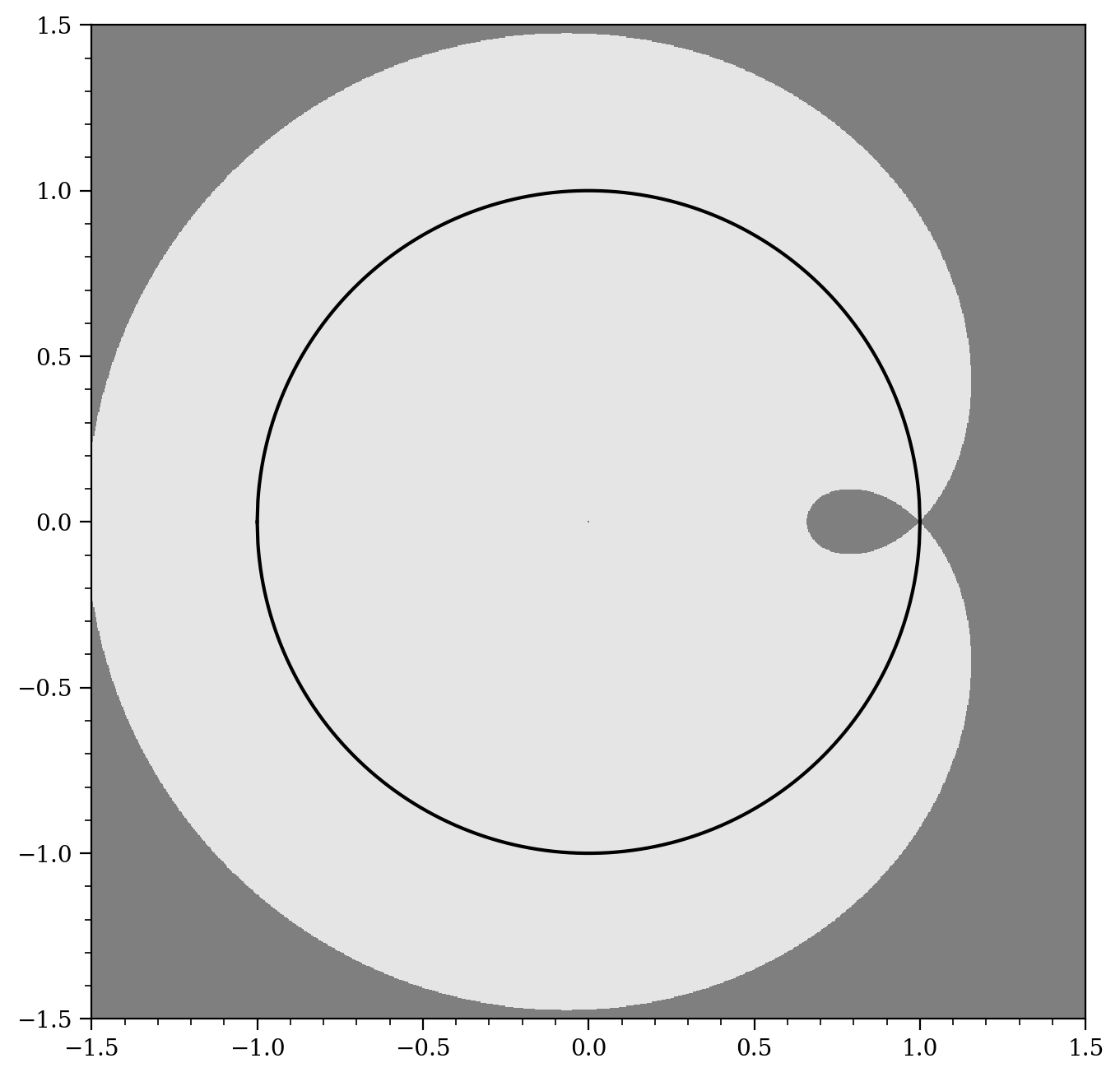
(a) The function $\mathfrak{D}_{*}$

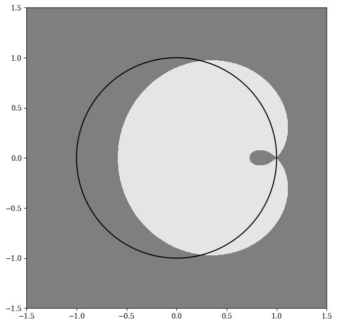
(b) The function $\mathfrak{H}_{*}$

Figure 7. The figures show where the designated function is larger (darker) or smaller (lighter) than 1 in absolute value, for $b_{1}=0.7$. The unit circle is shown for comparison.

Figure 7 shows the region in $\mathbb{C}$ where $|\mathfrak{D}_{*}(z)|<1$ and where $|\mathfrak{H}_{*}(z)|<1$, for $b_{1}=0.7$. In particular, we see that $|\mathfrak{H}_{*}(z)|<1$ fails for a portion of the unit circle $\mathcal{C}_{1}$. This being the case, we need to devise a different type of contour than the contour $\mathcal{C}_{r_{1}}$ used in the preceding subsection. We begin with a prototype

$$\mathcal{M}:=\{z:|z-\tfrac{1}{2}|=\tfrac{1}{2}\}.$$

This contour $\mathcal{M}$ satisfies the steepest decent condition

$$|\mathfrak{D}_{*}(z)|<1\text{ for all }z\in\mathcal{M}\setminus{\{1\}},\quad|\mathfrak{H}_{*}(z)|<1\text{ for all }z\in\mathcal{M}\setminus{\{1\}}, \mathcal{M}$$ (SD.)

which we verify now.

Proof of (SD.$\mathcal{M}$).

First, express $\mathfrak{D}_{*}(z)$ and $\mathfrak{H}_{*}(z)$ (defined in (6.8) and (6.24)) as

$$\mathfrak{D}_{*}(z) =\frac{b_{1}z+1-2b_{1}}{1-b_{1}z^{-1}}=1+\frac{b_{1}z+b_{1}z^{-1}-2b_{1}}{1-b_{1}z^{-1}}.$$

$$\mathfrak{H}_{*}(z) =\frac{b_{1}z+1-2b_{1}}{1-b_{1}z^{-1}}\frac{b_{1}(2-z^{-1})+1-2b_{1}}{1-b_{1}/(2-z^{-1})}=1+\frac{2b_{1}z+2b_{1}z^{-1}-4b_{1}}{2-b_{1}-z^{-1}}.$$

under the parametrization $z(\theta):=\frac{1+e^{\mathbf{i}\theta}}{2}\in\widetilde{\mathcal{C}}$, we calculate

$$\Big{|}\mathfrak{D}_{*}\Big{(}\frac{1+e^{\mathbf{i}\theta}}{2}\Big{)}\Big{|}^{2} =\Big{(}1+\frac{b_{1}(w-1)^{2}}{2(w+1-2b_{1})}\Big{)}\Big{(}1+\frac{b_{1}(w^{-1}-1)^{2}}{2(w^{-1}+1-2b_{1})}\Big{)}\Big{|}_{w=e^{\mathbf{i}\theta}}$$

$$=1+\frac{b_{1}(w-2+w^{-1})((2-3b_{1})(w+w^{-1})+4-2b_{1})}{|2(w^{-1}+1-2b_{1})|^{2}}\Big{|}_{w=e^{\mathbf{i}\theta}}$$

$$=1-\frac{b_{1}(1-\cos\theta)(2-b_{1}+(2-3b_{1})\cos\theta)}{|(w^{-1}+1-2b_{1})|^{2}}.$$

$$\Big{|}\mathfrak{H}_{*}\Big{(}\frac{1+e^{\mathbf{i}\theta}}{2}\Big{)}\Big{|}^{2} =\Big{(}1+\frac{b_{1}(w-1)^{2}}{(2-b_{1})w-b_{1}}\Big{)}\Big{(}1+\frac{b_{1}(w^{-1}-1)^{2}}{(2-b_{1})w^{-1}-b_{1}}\Big{)}\Big{|}_{w=e^{\mathbf{i}\theta}}$$

$$=1+\frac{4b_{1}(1-b_{1})(w-2+w^{-1})}{|(2-b_{1})w-b_{1}|^{2}}\Big{|}_{w=e^{\mathbf{i}\theta}}$$

$$=1-\frac{8b_{1}(1-b_{1})(1-\cos\theta)}{|(2-b_{1})e^{\mathbf{i}\theta}-b_{1}|^{2}}.$$

It is now readily checked that these expressions are strictly less than $1$ for all $\theta\in(\pi,\pi]\setminus{\{0\}}$ (and $b_{1}\in(0,1)$), which gives exactly the desired properties. ∎

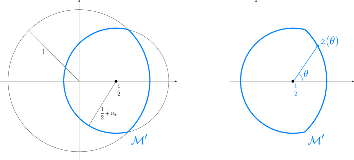
Figure 8. The contour $\mathcal{M}^{\prime}$ and its parametrization.

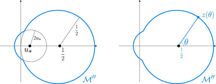
Figure 9. The contour $\mathcal{M}^{\prime\prime}$ and its parametrization.

Even though $\mathcal{M}$ enjoys the desired property (SD.$\mathcal{M}$), it cuts through the point $z=0$. This could cause issues, as the integrals (6.21)–(6.22) generally contain poles at $z_{1}=0$. To circumvent this problem, we consider modifications $\mathcal{M}^{\prime}$ and $\mathcal{M}^{\prime\prime}$ of $\mathcal{M}$:

$$\mathcal{M}^{\prime}=\mathcal{M}^{\prime}(u_{*}) :=\partial\big{(}\big{\{}|z|\leq 1\big{\}}\cap\big{\{}|z-\tfrac{1}{2}|\leq\tfrac{1}{2}+u_{*}\big{\}}\big{)},$$ (6.26)

$$\mathcal{M}^{\prime\prime}=\mathcal{M}^{\prime\prime}(u_{*}) :=\partial\big{(}\big{\{}|z-\tfrac{1}{2}|\leq\tfrac{1}{2}\big{\}}\cup\big{\{}|z-u_{*}|\leq 2u_{*}\big{\}}\big{)},$$ (6.27)

counterclockwise oriented; see Figures 8–9. Here $u_{*}\in(0,\frac{1}{12}\wedge b_{1})$ is a parameter, which we fix in Lemma 6.4 so that the resulting contours $\mathcal{M}^{\prime}$ and $\mathcal{M}^{\prime\prime}$ also enjoy the steepest decent condition. We now verify the steepest decent condition for $\mathcal{M}^{\prime}$ and $\mathcal{M}^{\prime\prime}$.

Lemma 6.4.

There exists $u_{*}\in(0,\frac{1}{12}\wedge b_{1})$ such that, for the contours $\mathcal{M}^{\prime}(u_{*})$ and $\mathcal{M}^{\prime\prime}(u_{*})$ we have

$$|\mathfrak{D}_{*}(z)|<1,\ |\mathfrak{H}_{*}(z)|<1\quad z\in\mathcal{M}^{\prime}\setminus{\{1\}}, \mathcal{M}^{\prime}$$ (SD.)

$$|\mathfrak{D}_{*}(z)|<1,\ |\mathfrak{H}_{*}(z)|<1\quad z\in\mathcal{M}^{\prime\prime}\setminus{\{1\}}. \mathcal{M}^{\prime\prime}$$ (SD.)

Proof.

We will show that for all small enough $u>0$,

$$|\mathfrak{D}_{*}(z)|<1,\ |\mathfrak{H}_{*}(z)|<1\quad z\in\mathcal{M}^{\prime}(u)\setminus{\{1\}},$$

$$|\mathfrak{D}_{*}(z)|<1,\ |\mathfrak{H}_{*}(z)|<1\quad z\in\mathcal{M}^{\prime\prime}(u)\setminus{\{1\}}.$$

We begin with the statement for $\mathcal{M}^{\prime\prime}(u)$. Indeed, this contour differs from $\mathcal{M}$ only in the neighborhood $O(3u):=\{z\in\mathbb{C}:|z|<3u\}$ of $z=0$. This being the case, instead of the entire contour $\mathcal{M}^{\prime\prime}(u)$, we need only to consider the part $\mathcal{M}^{\prime\prime}(u)\cap O(3u)$. We already know from (SD.$\mathcal{M}$) that $|\mathfrak{D}_{*}(0)|<1$ and $|\mathfrak{H}_{*}(0)|<1$. It is readily checked from (6.8) and (6.24) that $\mathfrak{D}_{*}(z)$ and $\mathfrak{H}_{*}(z)$ are continuous at $z=0$, hence we see that $|\mathfrak{D}_{*}(z)|<1,\ |\mathfrak{H}_{*}(z)|<1$ holds on $z\in\mathcal{M}^{\prime\prime}(u)\cap O(3u)$ for all small enough $u>0$.

We now turn to $\mathcal{M}^{\prime}(u)$. Let us first analyze the local behaviors of $\mathfrak{D}_{*}(z)$ and $\mathfrak{H}_{*}(z)$ near $z=1$. Straightforward calculation gives

$$\mathfrak{D}_{*}(1)=1, \partial_{z}\mathfrak{D}_{*}(1)=0, \partial^{2}_{z}\mathfrak{D}_{*}(1)=\nu_{*}, \mathfrak{H}_{*}(1)=1, \partial_{z}\mathfrak{H}_{*}(1)=0, \partial^{2}_{z}\mathfrak{H}_{*}(1)=2\nu_{*},$$

so Taylor expansion of $\mathfrak{D}_{*}(z)$ around $z=1$ gives $1+\frac{1}{2}\nu_{*}(z-1)^{2}$ up the second order, and Taylor expansion of $\mathfrak{H}_{*}(z)$ around $z=1$ gives $1+\nu_{*}(z-1)^{2}$ up the second order. The expression $\nu_{*}(z-1)^{2}$ is real and negative along the vertical direction: $z-1\in\mathbf{i}\mathbb{R}$. Since $\mathfrak{D}_{*}(z)$ and $\mathfrak{H}_{*}(z)$ are analytic in a neighborhood of $z=1$, we have

$$\big{|}\mathfrak{D}_{*}(z)\big{|},\ \big{|}\mathfrak{H}_{*}(z)\big{|}\leq 1-\tfrac{1}{C}|z-1|^{2},\quad\forall\,z\in\mathcal{A},$$

where $\mathcal{A}:=\{z=ve^{\mathbf{i}\phi}:v\in[0,v_{0}],|\phi\pm\tfrac{\pi}{2}|\leq\phi_{0}\}$ is an ‘hourglass-shape’ region centered at $z=1$, and $v_{0},\phi_{0}>0$ are fixed. See Figure 10. This property ensures that $|\mathfrak{D}_{*}|,|\mathfrak{H}_{*}|<1$ within $\mathcal{A}\setminus{\{1\}}$, so instead of the entire contour $\mathcal{M}^{\prime}(u)$, it suffices to consider the part $(\mathcal{M}^{\prime}(u)\setminus\mathcal{A})$.

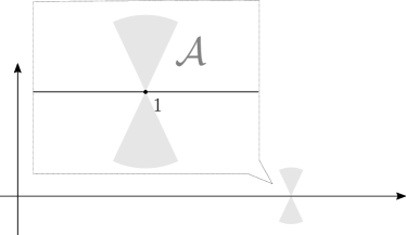
Figure 10. The hourglass-shape region $\mathcal{A}$.

Instead of $(\mathcal{M}^{\prime}(u)\setminus\mathcal{A})$, let us first consider $(\mathcal{M}\setminus\mathcal{A})$. Since the contour $\mathcal{M}$ passes through the point $z=1$ vertically, under the parametrization $z(\theta)=\frac{1+e^{\mathbf{i}\theta}}{2}$, the part $(\mathcal{M}\setminus\mathcal{A})$ avoids a neighborhood of $\theta=0$. This being the case, referring to the calculations (6.25), we see that

$$\sup_{z\in\mathcal{M}\setminus\mathcal{A}}|\mathfrak{D}_{*}(z)|<1,\quad\sup_{z\in\mathcal{M}\setminus\mathcal{A}}|\mathfrak{H}_{*}(z)|<1.$$

Let dist$(A,B):=\inf\{|z_{1}-z_{2}|:z_{1}\in A,z_{2}\in B\}$ denotes the distance of two sets $A,B\subset\mathbb{C}$. Referring to the definition (6.26) of $\mathcal{M}^{\prime}(u)$, we see that

$$\lim_{u\downarrow 0}\text{dist}\big{(}(\mathcal{M}\setminus\mathcal{A}),(\mathcal{M}^{\prime}(u)\setminus\mathcal{A})\big{)}=0.$$

Further, it is readily verified (from (6.8) and (6.24)) that $\mathfrak{D}_{*}$ and $\mathfrak{H}_{*}$ are uniformly continuous $\mathcal{M}$. These properties together give

$$\lim_{u\downarrow 0}\Big{(}\sup_{z\in\mathcal{M}^{\prime}(u)\setminus\mathcal{A}}|\mathfrak{D}_{*}(z)|\Big{)}=\sup_{z\in\mathcal{M}\setminus\mathcal{A}}|\mathfrak{D}_{*}(z)|<1, \lim_{u\downarrow 0}\Big{(}\sup_{z\in\mathcal{M}^{\prime}(u)\setminus\mathcal{A}}|\mathfrak{H}_{*}(z)|\Big{)}=\sup_{z\in\mathcal{M}\setminus\mathcal{A}}|\mathfrak{H}_{*}(z)|<1,$$

which concludes the proof. ∎

In the following subsections we prove Proposition 6.2(c)–(d), namely establishing the desired estimates on $\mathbf{V}^{\text{in}}_{\varepsilon}$ and its gradients. To this end, we treat separately the cases distinguished by the signs of $x_{2}-y_{1}$ and $x_{1}-y_{2}$, which we refer to as the $(+-)$, $(--)$, and $(++)$-cases:

• $x_{2}-y_{1}>0$ and $x_{1}-y_{2}\leq 0$, the $(+-)$-case;

• $x_{2}-y_{1}\leq 0$ and $x_{1}-y_{2}\leq 0$, the $(--)$-case;

• $x_{2}-y_{1}>0$ and $x_{1}-y_{2}>0$, the $(++)$-case.

The $(-+)$-case (i.e., $x_{2}-y_{1}\leq 0$ and $x_{1}-y_{2}>0$) is irrelevant due the assumption $x_{1}<x_{2}$ and $y_{1}<y_{2}$.

Let us introduce one more convention about Taylor expansion which will be used in the subsequent arguments. Recall the assumption $t\leq\varepsilon^{-2}T$ which ensures that $\varepsilon\leq C(T)(t+1)^{-1/2}$. At times we will Taylor expand expressions in the variables $(\sqrt{\varepsilon},\frac{1}{\sqrt{t+1}})$. In the course of doing so, we adopt the following ordering convention in light of the aforementioned condition on $\varepsilon$.

Definition 6.5.

To Taylor expand a given expression $f(\sqrt{\varepsilon},\frac{1}{\sqrt{t+1}})$, we assign $\sqrt{\varepsilon}$ the order of $(t+1)^{-1/4}$. For example, Taylor expansion of $f(\sqrt{\varepsilon},\frac{1}{\sqrt{t+1}})$ up to order $\frac{1}{\sqrt{t+1}}$ reads

$$f(0,0)+\partial_{1}f(0,0)\sqrt{\varepsilon}+\tfrac{1}{2}\partial^{2}_{1}f(0,0)\varepsilon+\partial_{2}f(0,0)\tfrac{1}{\sqrt{t+1}}.$$

6.3. Estimating the interacting part $\mathbf{V}^{\text{in}}_{\varepsilon}$, the $(+-)$-case

We begin by constructing the contour $\Gamma(t,\varepsilon)$. For the $(+-)$-case considered here, $\Gamma(t,\varepsilon)$ is constructed as perturbation of $\mathcal{M}^{\prime}$. More precisely, recall the definition of $\mathfrak{u}(t,\beta)$ from (6.6). For $\beta\in\mathbb{R}$, set

$$\mathcal{M}^{\prime}(t,\beta):=\partial\big{(}{\{|z|\leq\mathfrak{u}(t,\beta)\}}\cap{\{|z-\tfrac{1}{2}|\leq\tfrac{1}{2}\}}\big{)},$$ (6.28)

counterclockwise oriented; see Figure 11 and compare it with Figure 8. Under these notation, we set

$$\Gamma(t,\varepsilon):=\mathcal{M}^{\prime}(t,-k_{1}\alpha),$$

where $k_{1}=k_{1}(\alpha,T)\in\mathbb{Z}_{>0}$ is an auxiliary parameter to be fixed later.

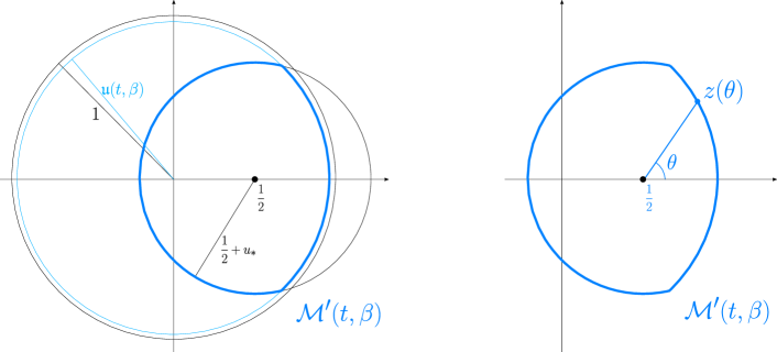
Figure 11. The contour $\mathcal{M}^{\prime}(t,\beta)$ and its parametrization. The figure shows the case $\beta<0$.

Hereafter we parametrize $z_{1}=z_{1}(\theta_{1})\in\mathcal{M}^{\prime}(t,-k_{1}\alpha)$ as depicted in Figure 11. As for the $z_{2}$-contour, we fix $k_{2}:=1$ in (6.17). Recalling $\widetilde{r}_{2}(z_{1})$ from (6.18), we parametrize $z_{2}(\theta):=\widetilde{r}_{2}(z_{1})e^{\mathbf{i}\theta_{2}}\in\mathcal{C}_{\widetilde{r}_{2}(z_{1})}$.

The parameter $k_{1}\in\mathbb{Z}_{>0}$ is to ensures that

$$r^{\prime}_{2}\geq\mathfrak{p}_{\varepsilon}(z_{1}(0))+\tfrac{1}{\sqrt{t+1}}\in\mathbb{R}.$$ (6.29)

To see why this holds for large enough $k_{1}$, recall from Definition 6.5 the announced convention on Taylor expansion, and expand the expression $r^{\prime}_{2}-\mathfrak{p}_{\varepsilon}(z_{1}(0))=\mathfrak{u}(t,2\alpha)-\mathfrak{p}_{\varepsilon}(\mathfrak{u}(t,-k_{1}\alpha))$ in $(\sqrt{\varepsilon},\frac{1}{\sqrt{t+1}})$ to the leading order in $\frac{1}{\sqrt{t+1}}$ to get

$$z_{2}(0)-\mathfrak{p}_{\varepsilon}(z_{1}(0))=0\cdot\sqrt{\varepsilon}-\rho(1-\rho)\varepsilon+\tfrac{(k_{1}+2)\alpha}{\sqrt{t+1}}+\ldots.$$

From this, together with $\varepsilon\leq\frac{C(T)}{\sqrt{t+1}}$ under current assumptions, we see that the condition (6.29) holds for a large enough $k_{1}=k_{1}(\alpha,T)$, and we fix such a $k_{1}\in\mathbb{Z}_{>0}$ hereafter.

The purpose of imposing the condition (6.29) is to control the region $\{z_{1}:|\mathfrak{p}_{\varepsilon}(z_{1})|>r^{\prime}_{2}\}$, as will be relevant toward controlling the integral $\mathbf{V}_{\text{res}}$ (6.22). Under the aforementioned parametrization $z_{1}=z_{1}(\theta)$, the condition (6.29) ensures a lower bound on $|\theta_{1}|$ for which $|\mathfrak{p}_{\varepsilon}(z_{1}(\theta))|>r^{\prime}_{2}$. That is,

$$|\mathfrak{p}_{\varepsilon}(z_{1}(\theta_{1}))|>r^{\prime}_{2}\text{ holds only if }|\theta_{1}|\geq\frac{1}{C(\alpha)(t+1)^{1/4}}.$$ (6.30)

Proof of (6.30).

Set $f(\theta_{1}):=|\mathfrak{p}_{\varepsilon}(z_{1}(\theta_{1}))|-r^{\prime}_{2}$. Our goal is to obtain a lower bound on those $|\theta_{1}|$ such that $f(\theta_{1})\geq 0$. Given the explicit expression $\mathfrak{p}_{\varepsilon}(z_{1}(\theta_{1}))=e^{\sqrt{\varepsilon}(\rho-1)}+e^{\sqrt{\varepsilon}\rho}-e^{\sqrt{\varepsilon}(2\rho-1)}\mathfrak{u}(t,k_{1}\alpha)e^{-\mathbf{i}\theta_{1}}$, one readily checks that $\frac{d~{}}{d\theta_{1}}f(0)=0$, and that $|\frac{d~{}}{d\theta_{1}}f(\theta_{1})|\leq C(\alpha)$, for all $(\theta_{1},t,\varepsilon)\in(-\pi,\pi]\times\mathbb{Z}_{\geq 0}\times(0,1)$. Taylor expanding $f(\theta_{1})$ accordingly as

$$f(\theta_{1})=f(0)+\int_{0}^{\theta_{1}}(\theta_{1}-\theta)\tfrac{d~{}}{d\theta}f(\theta)d\theta,$$

we see $f(\theta_{1})\geq 0$ only if $f(0)+C(\alpha)\theta_{1}^{2}\geq 0$. Now, the condition (6.29) ensures that $f(0)\leq-\frac{1}{\sqrt{t+1}}$. From this we conclude (6.30). ∎

Recall that $\mathfrak{H}_{\varepsilon}(t,z):=\mathfrak{D}_{\varepsilon}(t,z)\mathfrak{D}_{\varepsilon}(t,\mathfrak{p}_{\varepsilon}(z))$. Let us check that, along the contour $\mathcal{M}^{\prime}(t,-k_{1}\alpha)$, we do have the desired Gaussian decay of $|\mathfrak{D}_{\varepsilon}|$ and $|\mathfrak{H}_{\varepsilon}|$.

Lemma 6.6.

Given any $T\in(0,\infty)$ and $\beta\in\mathbb{R}$,

$$\big{|}\mathfrak{D}_{\varepsilon}(t,z)\big{|},\ \big{|}\mathfrak{H}_{\varepsilon}(t,z)\big{|}\leq C(\beta,T)\exp(-\tfrac{\theta^{2}}{C}(t+1)),\quad z=z(\theta)\in\mathcal{M}^{\prime}(t,\beta),$$

for all $\theta\in(-\pi,\pi]$, large enough $t\leq\varepsilon^{-2}T$, and small enough $\varepsilon>0$.

Proof.

The proof follows the same three-step procedure as the proof of Lemma 6.3. Given the identities (6.9a)–(6.9c), the proof of the first two steps (Zero $\theta$)–(Small $\theta$) follows the same argument via Taylor expansion as in Lemma 6.3, and we do not repeat it here.

We now focus on establishing the last step (Large $\theta$). First, the contour $\mathcal{M}^{\prime}(t,\beta)$ converges, as $t\to\infty$, to $\mathcal{M}^{\prime}$. More precisely, write $z_{\mathcal{M}^{\prime}(t,\beta)}(\theta;t,\beta)$ and $z_{\mathcal{M}^{\prime}}(\theta)$ for the respectively polar parametrization as depicted in Figures 11 and 8. We have $\lim_{t\to\infty}z_{\mathcal{M}^{\prime}(t,\beta)}(\theta;t,\beta)=z_{\mathcal{M}^{\prime}}(\theta)$, uniformly over $\theta\in(-\pi,\pi]$. This being the case, from the given expressions (6.7)–(6.8), (6.19) and (6.24) of $\mathfrak{D}_{\varepsilon}(t,z)$, $\mathfrak{D}_{*}(z)$, $\mathfrak{H}_{\varepsilon}(z)$, and $\mathfrak{H}_{*}(z)$, it is readily checked that

$$\lim_{t\to\infty}\big{|}\mathfrak{D}_{\varepsilon}(t,z_{\mathcal{M}^{\prime}(t,\beta)}(\theta))\big{|}^{\frac{1}{t}} =\big{|}\mathfrak{D}_{*}(z_{\mathcal{M}^{\prime}}(\theta))\big{|},$$

$$\lim_{t\to\infty}\big{|}\mathfrak{H}_{\varepsilon}(t,z_{\mathcal{M}^{\prime}(t,\beta)}(\theta))\big{|}^{\frac{1}{t}} =\big{|}\mathfrak{H}_{*}(z_{\mathcal{M}^{\prime}}(\theta))\big{|},$$

uniformly over $\theta\in(-\pi,\pi]$. The limiting expressions on the r.h.s. put us into the considerations of the steepest decent condition (SD.$\mathcal{M}^{\prime}$), which has been verified in Lemma 6.4. From this we conclude the desired conclusion: there exists $t_{0}<\infty$ such that, for any given $\theta_{0}>0$,
$\hphantom{aaaaa}\displaystyle\big{|}\mathfrak{D}_{\varepsilon}(t,z)\big{|}^{\frac{1}{t}}\leq 1-\tfrac{1}{C(\theta)},\quad\big{|}\mathfrak{D}_{\varepsilon}(t,z)\big{|}^{\frac{1}{t}}\leq 1-\tfrac{1}{C(\theta)},\quad\forall z=z_{\mathcal{M}^{\prime}(t,\beta)}(\theta)\in\mathcal{M}^{\prime}(t,\beta),\ |\theta|\geq\theta_{0}.$ ∎

We have all the necessary ingredients for estimating $\mathbf{V}^{\text{in}}_{\varepsilon}$.

Proof of Proposition 6.2(c)–(d), the $(+-)$-case, with large enough $t$.

The proof begins with the contour deformation described in Section 6.2. Let us check the condition (No Pole). For a fixed $z_{2}\in\mathcal{C}_{r}$, the integrand in (6.4) has poles in $z_{1}=0$, $z_{1}=e^{\sqrt{\varepsilon}(\rho-1)}b_{1}$, and $\mathfrak{p}_{\varepsilon}(z_{1})=z_{2}$. Referring to the definition (6.28) of $\mathcal{M}^{\prime}(t,-k_{1}\alpha)$ (or Figure 11), we see that the first two poles are contained in $\mathcal{M}^{\prime}(t,-k_{1}\alpha)$. As for the pole $\mathfrak{p}_{\varepsilon}(z_{1})=z_{2}$, the function $\mathfrak{p}_{\varepsilon}(z)$ (defined in (6.16)) is uniformly bounded (in $(\varepsilon,z)$) away from $z=0$. This being the case, by making $r$ large enough, we ensure that $|\mathfrak{p}_{\varepsilon}(z_{1})|<r=|z_{2}|$ throughout the contour deformation $z_{1}\in\mathcal{C}_{r}\mapsto\mathcal{M}^{\prime}(t,-k_{1}\alpha)$. Having checked the condition (No Pole), we are now given the decomposition $\mathbf{V}^{\text{in}}_{\varepsilon}=\mathbf{V}_{\text{blk}}+\mathbf{V}_{\text{res}}$. The proof amounts to bounding $\mathbf{V}_{\text{blk}}$ and $\mathbf{V}_{\text{res}}$, as well as their gradients.

We begin with $\mathbf{V}_{\text{blk}}$ (6.21). The proof consists of a sequence of bounds on terms appearing in the integrand (6.21). In the following we assume $z_{1}=z_{1}(\theta_{1})\in\mathcal{M}^{\prime}(t,-k_{1}\alpha)$ and $z_{2}=z_{1}(\theta_{2})\in\mathcal{C}_{\widetilde{r}_{2}(z_{1})}$.

• Show that $|z_{1}|^{x_{2}-y_{1}+\mu_{\varepsilon}t-\lfloor\mu_{\varepsilon}t\rfloor}\leq\exp(-\frac{\alpha|x_{2}-y_{1}|}{\sqrt{t+1}+C(\alpha)})$:
  Referring to the definition (6.28) of $\mathcal{M}^{\prime}(t,-k_{1}\alpha)$ (or Figure 11), we see that $\mathcal{M}^{\prime}(t,-k_{1}\alpha)$ is contained in $\mathcal{C}_{\mathfrak{u}(t,-k_{1}\alpha)}$, so

  $$|z_{1}|^{x_{2}-y_{1}+\mu_{\varepsilon}t-\lfloor\mu_{\varepsilon}t\rfloor}\leq\mathfrak{u}(t,-k_{1}\alpha)^{|x_{2}-y_{1}|}\leq C(\alpha)e^{-\frac{\alpha|x_{2}-y_{1}|}{\sqrt{t+1}+C(\alpha)}}.$$

• Show that $|z_{2}|^{x_{1}-y_{2}+\mu_{\varepsilon}t-\lfloor\mu_{\varepsilon}t\rfloor}\leq C(\alpha)\exp(-\frac{\alpha|x_{1}-y_{2}|}{\sqrt{t+1}+C(\alpha)})$:
  Recall the current assumption $x_{1}-y_{2}\leq 0$. The power $x_{1}-y_{2}+\mu_{\varepsilon}t-\lfloor\mu_{\varepsilon}t\rfloor$ would have a definitive sign (i.e., non-positive) if we offset it by $-(\mu_{\varepsilon}t-\lfloor\mu_{\varepsilon}t\rfloor)$. Since $|z_{2}|\leq C(\alpha)$ is bounded along its contour $z_{2}\in\mathcal{C}_{\widetilde{r}_{2}(z_{1})}$, offsetting the exponent costs only a factor of $C(\alpha)$:

  $$|z_{2}|^{x_{1}-y_{2}+\mu_{\varepsilon}t-\lfloor\mu_{\varepsilon}t\rfloor}\leq C(\alpha)|z_{2}|^{x_{1}-y_{2}}=C(\alpha)|z_{2}|^{-|x_{1}-y_{2}|}.$$

  Recall the definitions of the $r_{2}$’s and of $\widetilde{r}_{2}$ from (6.17)–(6.18), and recall that $k_{2}:=1$ here. We see that $\widetilde{r}_{2}(z_{2})\geq\mathfrak{u}(t,\alpha)$, so

  $$|z_{2}|^{x_{1}-y_{2}+\mu_{\varepsilon}t-\lfloor\mu_{\varepsilon}t\rfloor}\leq C(\alpha)\mathfrak{u}(t,\alpha)^{-|x_{1}-y_{2}|}\leq C(\alpha)e^{\frac{-\alpha|x_{1}-y_{2}|}{\sqrt{t+1}+C(\alpha)}}.$$

• Show that $|\mathfrak{F}_{\varepsilon}(z_{1},z_{2})|\leq C(\alpha)(1+|\theta_{1}|\sqrt{t+1}+|\theta_{2}|\sqrt{t+1})$:
  Recall the expression (6.15) of $\mathfrak{F}_{\varepsilon}$, and rewrite it as

  $$\mathfrak{F}_{\varepsilon}(z_{1},z_{2})=1+\big{(}e^{\sqrt{\varepsilon}(\rho-1)}+e^{\sqrt{\varepsilon}\rho}\big{)}\frac{z_{2}/z_{1}-1}{z_{2}-\mathfrak{p}_{\varepsilon}(z_{1})}.$$ (6.31)

  Referring to the definition (6.28) of $\mathcal{M}^{\prime}(t,-k_{1}\alpha)$ (or Figure 11), we see that $\mathcal{M}^{\prime}(t,-k_{1}\alpha)$ coincides with the circle $\mathcal{C}_{\mathfrak{u}(t,-k_{1}\alpha)}$ for small $\theta_{1}$, i.e., $|\theta_{1}|\leq\phi_{1}^{*}$, fixed $\phi^{*}_{1}>0$. Also $z_{2}(\theta_{2})=\widetilde{r}_{2}(z_{1})e^{\mathbf{i}\theta_{2}}=\mathfrak{u}(t,(2\pm 1)\alpha)e^{\mathbf{i}\theta_{2}}$, where the $\pm$ depends on whether $\mathfrak{p}_{\varepsilon}(z_{1}(\theta_{1}))>r^{\prime}_{2}$ or not. Taylor expanding $(z_{2}/z_{1}-1)$ in $\theta_{1},\theta_{2}$ then yields

  $$|z_{2}/z_{1}-1| \leq\tfrac{C(\alpha)}{\sqrt{t+1}}+C(\alpha)|\theta_{2}-\theta_{1}|$$

  $$\leq\tfrac{C(\alpha)}{\sqrt{t+1}}+C(\alpha)|\theta_{1}|+C(\alpha)|\theta_{2}|.$$ (6.32)

  for all $\theta_{1}$ and $\theta_{2}$ small enough. Further, since both $|z_{1}|$ and $|z_{2}|$ are bounded away from $0$ and $\infty$ along their relevant contours, the bound (6.32) actually extends to all values of $\theta_{1},\theta_{2}$. Using (6.32) and (6.23) on the r.h.s. of (6.31), we conclude the desired bound on $|\mathfrak{F}_{\varepsilon}(z_{1},z_{2})|$.

• Show that $|\mathfrak{D}_{\varepsilon}(z_{i})|\leq C(\alpha,T)\exp(-\frac{\theta^{2}_{i}}{C}(t+1))$:
  This is the content of Lemma 6.6.

Expressing (6.21) as an integral over $(\theta_{1},\theta_{2})\in(-\pi,\pi]^{2}$, and inserting the bounds from ($\mathbf{V}_{\text{blk}}$.$z_{1}$)–($\mathbf{V}_{\text{blk}}$.$\mathfrak{D}_{\varepsilon}$) into the resulting expression, we arrive at

$$|\mathbf{V}_{\text{blk}}|\leq C(\alpha,T)\int_{-\pi}^{\pi}\int_{-\pi}^{\pi}e^{-\frac{\alpha(|x_{2}-y_{1}|+|x_{1}-y_{2}|)}{\sqrt{t+1}+C(\alpha)}}(1+\sqrt{t+1}|\theta_{1}|+\sqrt{t+1}|\theta_{2}|)e^{-\frac{1}{C}(t+1)\theta_{i}^{2}}d\theta_{i}.$$

Performing the change of variables $\sqrt{t+1}\theta_{i}\mapsto\theta_{i}$, and extending the integration domain to $\mathbb{R}^{2}$ (which only increases its value) we obtain the desired bound on $|\mathbf{V}_{\text{blk}}|$:

$$|\mathbf{V}_{\text{blk}}|\leq C(\alpha,T)e^{-\frac{\alpha(|x_{2}-y_{1}|+|x_{1}-y_{2}|)}{\sqrt{t+1}+C(\alpha)}}\frac{1}{t+1}\int_{\mathbb{R}^{2}}(1+|\theta_{1}|+|\theta_{2}|)e^{-\frac{1}{C}\theta_{i}^{2}}d\theta_{i}=\frac{C(\alpha,T)}{t+1}e^{-\frac{\alpha(|x_{2}-y_{1}|+|x_{1}-y_{2}|)}{\sqrt{t+1}+C(\alpha)}}.$$

As for $\mathbf{V}_{\text{res}}$, the proof similarly consists of bounds on terms involved in the integral (6.22). In the following we always assume $z_{1}=z_{1}(\theta_{1})\in\mathcal{M}^{\prime}(t,-k_{1}\alpha)$.

• Show that $\frac{1}{|\mathfrak{p}_{\varepsilon}(z_{1})||z_{1}|}\leq C(\alpha)$:
  Referring to the definition (6.28) of $\mathcal{M}^{\prime}(t,-k_{1}\alpha)$ (or Figure 11), we see that $|z_{1}|$ is bounded away from $0$ and $\infty$ along $\mathcal{M}^{\prime}(t,-k_{1}\alpha)$. This being the case, referring to the definition (6.16) of $\mathfrak{p}_{\varepsilon}(z)$, we see that the same holds for $|\mathfrak{p}_{\varepsilon}(z_{1})|$. Hence the claim follows.

• Show that $\mathbf{1}_{{\{|\mathfrak{p}_{\varepsilon}(z_{1})|>r^{\prime}_{2}\}}}|\mathfrak{J}(z_{1})|\leq\exp(-\frac{\alpha(|x_{2}-y_{1}|+|x_{1}-y_{2}|)}{\sqrt{t+1}+C(\alpha)})$:
  Recall from (6.20) that $\mathfrak{J}(z_{1})$ consists of products of powers of $z_{1}$ and $\mathfrak{p}_{\varepsilon}(z_{1})$. As argued in the previous step ($\mathbf{V}_{\text{res}}$.$\frac{1}{z_{1}\mathfrak{p}_{\varepsilon}}$), the terms $|z_{1}|,|z_{1}|^{-1},|\mathfrak{p}_{\varepsilon}(z_{1})|,|\mathfrak{p}_{\varepsilon}(z_{1})|^{-1}\leq C(\alpha)$ are bounded along $\mathcal{M}^{\prime}(t,-k\alpha_{1})$. This being the case, we alter the powers in (6.20) by some fixed amount, at the cost of $C(\alpha)$, and write

  $$\mathbf{1}_{{\{|\mathfrak{p}_{\varepsilon}(z_{1})|>r^{\prime}_{2}\}}}|\mathfrak{J}(z_{1})|\leq C(\alpha)\mathbf{1}_{{\{|\mathfrak{p}_{\varepsilon}(z_{1})|>r^{\prime}_{2}\}}}|z_{1}|^{|x_{2}-y_{1}|}|\mathfrak{p}_{\varepsilon}(z_{1})|^{-|x_{1}-y_{2}|}.$$

  In the last expression, using $|z_{1}|\leq\mathfrak{u}(t,-k_{1}\alpha)$ (as argued in ($\mathbf{V}_{\text{blk}}$.$z_{1}$)) and the given constraint $|\mathfrak{p}_{\varepsilon}(z_{1})|>r^{\prime}_{2}=\mathfrak{u}(t,2\alpha)$, we obtained the desired property:

  $$\mathbf{1}_{{\{|\mathfrak{p}_{\varepsilon}(z_{1})|>r^{\prime}_{2}\}}}|\mathfrak{J}(z_{1})|\leq C(\alpha)\mathfrak{u}(t,-k_{1}\alpha)^{|x_{2}-y_{1}|}\mathfrak{u}(t,\alpha)^{-|x_{1}-y_{2}|}\leq C(\alpha)e^{-\frac{\alpha(|x_{2}-y_{1}|+|x_{1}-y_{2}|)}{\sqrt{t+1}+C(\alpha)}}.$$

• Show that $|\mathfrak{H}_{\varepsilon}(z_{1})|\leq C(\alpha,T)\exp(-\frac{\theta^{2}_{1}}{C}(t+1))$:
  This is the content of Lemma 6.6.

Express (6.22) as an integral over $\theta_{1}\in(-\pi,\pi]$, and insert the bounds from ($\mathbf{V}_{\text{res}}$.$\frac{1}{z_{1}\mathfrak{p}_{\varepsilon}}$)–($\mathbf{V}_{\text{res}}$.$\mathfrak{H}_{\varepsilon}$) into the resulting expression. This together the derived lower bound (6.30) on $|\theta_{1}|$ gives

$$|\mathbf{V}_{\text{res}}|\leq C(\alpha,T)e^{-\frac{\alpha(|x_{2}-y_{1}|+|x_{1}-y_{2}|)}{\sqrt{t+1}+C(\alpha)}}\int_{(-\pi,\pi]}\mathbf{1}\{|\theta_{1}|\geq\tfrac{1}{C(\alpha)(t+1)^{1/4}}\}e^{-\frac{1}{C}(t+1)\theta_{1}^{2}}d\theta_{1}.$$

Extending the integration domain to $\mathbb{R}$, and performing a change of variable $\sqrt{t+1}\theta_{1}\mapsto\theta_{1}$ yields

$$|\mathbf{V}_{\text{res}}|\leq C(\alpha,T)e^{-\frac{\alpha(|x_{2}-y_{1}|+|x_{1}-y_{2}|)}{\sqrt{t+1}+C(\alpha)}}\frac{1}{\sqrt{t+1}}\int_{\mathbb{R}}\mathbf{1}\{|\theta_{1}|\geq\tfrac{(t+1)^{1/4}}{C(\alpha)}\}e^{-\frac{1}{C}\theta_{1}^{2}}d\theta_{1}.$$

Here, unlike in the case for $\mathbf{V}^{\text{fr}}_{\varepsilon}$, we get $\frac{1}{\sqrt{t+1}}$ instead of $\frac{1}{t+1}$ in front of the integral. This insufficiency is compensated by having the constraint $|\theta_{1}|\geq(t+1)^{1/4}/C(\alpha)$. Indeed,

$$\int_{\mathbb{R}}\mathbf{1}\{|\theta_{1}|\geq\tfrac{(t+1)^{1/4}}{C(\alpha)}\}e^{-\frac{1}{C}\theta_{1}^{2}}d\theta_{1}\leq\exp\big{(}-\tfrac{1}{C(\alpha)}(t+1)^{1/4}\big{)},$$

and fractional exponentials such as $\exp(-\frac{1}{C(\alpha)}(t+1)^{1/4})$ decay faster than any power $(t+1)^{-n}$. From this we conclude the desired bound on $|\mathbf{V}_{\text{res}}|$:

$$|\mathbf{V}_{\text{res}}|\leq\frac{C(\alpha,T)}{t+1}e^{-\frac{\alpha(|x_{2}-y_{1}|+|x_{1}-y_{2}|)}{\sqrt{t+1}+C(\alpha)}}.$$

So far we have derived bounds on $|\mathbf{V}_{\text{blk}}|$ and $|\mathbf{V}_{\text{res}}|$, and this concludes the proof of Proposition 6.2(c). Part (d) amounts to performing similar estimates on the gradients, e.g., $|\nabla_{x_{j}}\mathbf{V}_{\text{blk}}|$ and $|\nabla_{x_{j}}\mathbf{V}_{\text{res}}|$. Taking a gradient merely introduces a factor of $(z_{j}^{\pm}-1)$ in the contour integrals (6.21)–(6.22). It is straightforward to check that

$$|z_{j}^{\pm}-1|\leq\tfrac{1}{\sqrt{t+1}}+|\theta_{j}|,\quad z_{1}=z_{1}(\theta)\in\mathcal{M}^{\prime}(t,-k_{1}\alpha),\quad z_{2}=z_{2}(\theta)\in\mathcal{C}_{\widetilde{r}_{2}(z_{1})}.$$ (6.33)

Incorporate this bound into the preceding analysis gives the desired bounds on the gradients. Compared to the bounds on $|\mathbf{V}_{\text{blk}}|$ and $|\mathbf{V}_{\text{res}}|$, an additional factor of $\frac{1}{\sqrt{t+1}}$ arises due to (6.33). ∎

6.4. Estimating the interacting part $\mathbf{V}^{\text{in}}_{\varepsilon}$, the $(--)$-case

The case considered here is more involved than the $(+-)$-case: we face a conflict in the choice of the $z_{1}$-contour. As discussed in Section 6.2, in order to control the term $\mathfrak{H}_{\varepsilon}(t,z)$ in $\mathbf{V}_{\text{res}}$ by steepest decent analysis, we favor contours of the type $\mathcal{M}^{\prime}(t,\beta)$. On the other hand, with $x_{2}-y_{1}\leq 0$ under current assumptions, we need $|z_{1}|>1$ in $\mathbf{V}_{\text{blk}}$ to obtain the desired spatial exponential decay $\exp(-\frac{\alpha|x_{2}-y_{1}|}{\sqrt{t+1}+C(\alpha)})$. Referring to the definition (6.28) of $\mathcal{M}^{\prime}(t,-k_{1}\alpha)$ (or Figure 11), we see that $|z_{1}|>1$ fails for a portion of $\mathcal{M}^{\prime}(t,\beta)$, regardless of the sign of $\beta$—i.e., the bulk part $\mathbf{V}_{\text{blk}}$ and the residue part $\mathbf{V}_{\text{res}}$ favor different contours.

In view of the preceding discussion, we choose

$$\Gamma(t,\varepsilon):=\mathcal{C}_{\mathfrak{u}(t,3\alpha)},$$

which is preferred for controlling $\mathbf{V}_{\text{blk}}$ but not $\mathbf{V}_{\text{res}}$, and then, re-deforming contour $\mathcal{C}_{\mathfrak{u}(t,3\alpha)}\mapsto\mathcal{M}^{\prime}(t,3\alpha)$ in $\mathbf{V}_{\text{res}}$. Let us check that doing so does not cross a pole.

Lemma 6.7.

For all $t>0$ large enough and $\varepsilon>0$ small enough, we have $\mathbf{V}_{\text{res}}=\mathbf{V}_{\text{res}}^{\prime}$, where

$$\mathbf{V}_{\text{res}}^{\prime} :=\oint_{\mathcal{M}^{\prime}(t,3\alpha)}\mathbf{1}_{{\{|\mathfrak{p}_{\varepsilon}(z_{1})|>r^{\prime}_{2}\}}}\mathfrak{J}(z_{1})\frac{1}{z_{1}\mathfrak{p}_{\varepsilon}(z_{1})}\mathfrak{H}_{\varepsilon}(t,z_{1})dz_{1}$$ (6.34)

is the same as $\mathbf{V}_{\text{res}}$ except the contour is replaced by $\mathcal{M}^{\prime}(t,3\alpha)$.

Proof.

Referring to the definition (6.28) of $\mathcal{M}^{\prime}(t,3\alpha)$ (or Figure 11), we see that the difference $\mathcal{C}_{\mathfrak{u}(t,3\alpha)}-\mathcal{M}^{\prime}(t,3\alpha)$ is the boundary of the crescent

$$\mathcal{G}(t):=\big{\{}z\in\mathbb{C}:|z|\leq\mathfrak{u}(t,3\alpha)\big{\}}\setminus\big{\{}z\in\mathbb{C}:|z-\tfrac{1}{2}|<\tfrac{1}{2}+u_{*}\big{\}}.$$

See Figure 12. We write $\partial\mathcal{G}(t)$ for the boundary, counterclockwise oriented. This gives

$$\mathbf{V}_{\text{res}}-\mathbf{V}_{\text{res}}^{\prime}=\frac{e^{\sqrt{\varepsilon}(\rho-1)}+e^{\sqrt{\varepsilon}\rho}}{2\pi\mathbf{i}}\oint_{\partial\mathcal{G}(t)}\mathbf{1}_{{\{|\mathfrak{p}_{\varepsilon}(z_{1})|>r^{\prime}_{2}\}}}\mathfrak{J}(z_{1})\frac{1}{z_{1}\mathfrak{p}_{\varepsilon}(z_{1})}\mathfrak{H}_{\varepsilon}(t,z_{1})dz_{1}.$$

Along $\partial\mathcal{G}(t)$, the indicator $\mathbf{1}_{{\{|\mathfrak{p}_{\varepsilon}(z_{1})|>r^{\prime}_{2}\}}}$ is in fact irrelevant. More precisely, setting

$$\mathcal{H}(t,\varepsilon,\beta):=\{|\mathfrak{p}_{\varepsilon}(z)|\leq\mathfrak{u}(t,\beta)\},$$ (6.35)

let us check that

$$\text{ given any }\beta\in\mathbb{R}\text{ and }u>0,\ \mathcal{H}(t)\subset\big{\{}|z-\tfrac{1}{2}|\leq\tfrac{1}{2}+u\big{\}},$$ (6.36)

for all $t$ large enough and $\varepsilon$ small enough. Referring to the definition (6.16) of $\mathfrak{p}_{\varepsilon}(z)$, we have $\lim_{\varepsilon\to 0}\mathfrak{p}_{\varepsilon}(z):=\mathfrak{p}_{*}(z)=2-z^{-1}$. Consider $\mathcal{H}_{*}:=\{z\in\mathbb{C}:|\mathfrak{p}_{*}(z)|\leq 1\}$, which is the $(t,\varepsilon)\to(\infty,\varepsilon)$ limit of $\mathcal{H}(t,\varepsilon,\beta)$. Indeed, along the contour $\mathcal{M}:=\frac{1}{2}+\mathcal{C}_{\frac{1}{2}}$,we have $|z\mathfrak{p}_{*}(z)|=2|z-\frac{1}{2}|=1$ and $|z|>1$ except when $z=1$. Consequently, $\mathcal{M}\cap\mathcal{H}_{*}=\{1\}$. Also, it is readily checked that $\frac{1}{2}\in\mathcal{H}_{*}$ and that $\mathcal{H}_{*}$ is connected. From these properties, we deduce that $\mathcal{H}_{*}\subset\{|z-\frac{1}{2}|\leq\frac{1}{2}\}$. Since $\mathcal{H}_{*}$ is the $(t,\varepsilon)\to(\infty,0)$ limit of $\mathcal{H}(t,\varepsilon,\beta)$, for all $t$ large enough and $\varepsilon$ small enough, the claim (6.36) follows.

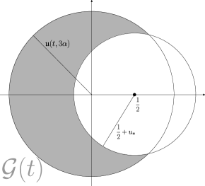
Figure 12. The region $\mathcal{G}(t)$.

Given (6.36), we drop the indicator $\mathbf{1}_{{\{|\mathfrak{p}_{\varepsilon}(z_{1})|>r^{\prime}_{2}\}}}$ and write

$$\mathbf{V}_{\text{res}}^{\prime}-\mathbf{V}_{\text{res}}=\frac{e^{\sqrt{\varepsilon}(\rho-1)}+e^{\sqrt{\varepsilon}\rho}}{2\pi\mathbf{i}}\oint_{\partial\mathcal{G}(t)}\frac{\mathfrak{J}(z_{1})}{z_{1}\mathfrak{p}_{\varepsilon}(z_{1})}\mathfrak{H}_{\varepsilon}(t,z_{1})dz_{1}.$$

Our goal is to show that the integral is zero. To this end, set $\mathfrak{q}_{\varepsilon}(z):=z\mathfrak{p}_{\varepsilon}(z):=(e^{\sqrt{\varepsilon}\rho}+e^{\sqrt{\varepsilon}(\rho-1)})z-e^{\sqrt{\varepsilon}(2\rho-1)}$, recall the definition of $\mathfrak{J}(z_{1})$ from (6.20), that $\mathfrak{H}_{\varepsilon}(t,z_{1}):=\mathfrak{D}_{\varepsilon}(t,z_{1})\mathfrak{D}_{\varepsilon}(t,\mathfrak{p}_{\varepsilon}(z_{1}))$, and recall the definition of $\mathfrak{D}_{\varepsilon}(t,z)$ from (4.14). We express the integrand of the last integral as

$$\frac{\mathfrak{J}(z_{1})}{z_{1}\mathfrak{p}_{\varepsilon}(z_{1})}\mathfrak{H}_{\varepsilon}(t,z_{1})= \big{(}z_{1}^{(x_{2}-y_{1})-(x_{1}-y_{2})-2+(\mu_{\varepsilon}t-\lfloor\mu_{\varepsilon}t\rfloor)}-z_{1}^{(x_{2}-y_{1})-(x_{1}-y_{2})+(\mu_{\varepsilon}t-\lfloor\mu_{\varepsilon}t\rfloor)}\big{)}\mathfrak{q}_{\varepsilon}(z_{1})^{x_{1}-y_{2}-1+\lfloor\mu_{\varepsilon}t\rfloor},$$

$$\Big{(}\lambda_{\varepsilon}\Big{(}\frac{z_{1}b_{1}+(1-b_{1}-b^{\varepsilon}_{2})\tau_{\varepsilon}^{-\rho}}{z_{1}-b^{\varepsilon}_{2}\tau_{\varepsilon}^{-\rho}}\Big{)}\Big{)}^{t}\Big{(}\lambda_{\varepsilon}\Big{(}\frac{\mathfrak{p}_{\varepsilon}(z_{1})b_{1}+(1-b_{1}-b^{\varepsilon}_{2})\tau_{\varepsilon}^{-\rho}}{\mathfrak{p}_{\varepsilon}(z_{1})-b^{\varepsilon}_{2}\tau_{\varepsilon}^{-\rho}}\Big{)}\Big{)}^{t}.$$ (6.37)

It suffices to check that this expression has no poles within $z_{1}\in\mathcal{G}(t)$. The assumption $x_{1}<x_{2}$ and $y_{1}<y_{2}$ ensures that $(x_{2}-y_{1})-(x_{1}-y_{2})\geq 2$. Thus, the expression (6.37) can only have poles at $\mathfrak{q}_{\varepsilon}^{-1}(0)$, $b^{\varepsilon}_{2}\tau_{\varepsilon}^{-\rho}$, or $\mathfrak{p}_{\varepsilon}^{-1}(b^{\varepsilon}_{2}\tau_{\varepsilon}^{-\rho})$. With $b^{\varepsilon}_{2}\to b_{1}$, $\tau_{\varepsilon}\to 1$, and $\mathfrak{p}_{\varepsilon}(z)\to 2-z^{-1}$, we have

$$\mathfrak{q}_{\varepsilon}^{-1}(0)\longrightarrow\tfrac{1}{2},\quad b^{\varepsilon}_{2}\tau_{\varepsilon}^{-\rho}\longrightarrow b_{1},\quad\mathfrak{p}_{\varepsilon}^{-1}(b^{\varepsilon}_{2}\tau_{\varepsilon}^{-\rho})\longrightarrow\tfrac{1}{2-b_{1}},\quad\text{as }\varepsilon\to 0.$$

Referring to Figure 12, we see that $\frac{1}{2}$, $b_{1}$, and $\frac{1}{2-b_{1}}$, all sit strictly outside of $\mathcal{G}(t)$. Consequently, no poles enter into $\mathcal{G}(t)$ as long as $t>0$ is large enough and $\varepsilon>0$ is small enough. ∎

Having introduced the contours $\mathcal{C}_{\mathfrak{u}(t,3\alpha)}$ and $\mathcal{M}^{\prime}(t,3\alpha)$, hereafter we write $z_{1}(\theta_{1})=\mathfrak{u}(t,3\alpha)e^{\mathbf{i}\theta_{1}}\in\mathcal{C}_{\mathfrak{u}(t,3\alpha)}$, and write $\widetilde{z}_{1}(\theta_{1})\in\mathcal{M}^{\prime}(t,3\alpha)$ for the parametrization depicted in Figure 11.

To control $\mathbf{V}_{\text{res}}$ in the following, similarly to the $(+-)$-case done previously, we need the analogous condition (6.29) to hold:

$$r^{\prime}_{2}\geq\mathfrak{p}_{\varepsilon}(\widetilde{z}_{1}(0))+\tfrac{1}{\sqrt{t+1}}\in\mathbb{R}.$$ (6.29’)

We achieve this by making the auxiliary parameter $k_{2}\in\mathbb{Z}_{>0}$ in (6.17) large enough. Recall from Definition 6.5 the announced convention on Taylor expansion, and expand the expression $r^{\prime}_{2}-\mathfrak{p}_{\varepsilon}(\widetilde{z}_{1}(0))=\mathfrak{u}(t,2k_{2}\alpha)-\mathfrak{p}_{\varepsilon}(\mathfrak{u}(t,3\alpha))$ in $(\sqrt{\varepsilon},\frac{1}{\sqrt{t+1}})$ to the leading order in $\frac{1}{\sqrt{t+1}}$ to get

$$z_{2}(0)-\mathfrak{p}_{\varepsilon}(\widetilde{z}_{1}(0))=0\cdot\sqrt{\varepsilon}-\rho(1-\rho)\varepsilon+\tfrac{(k_{2}-3)\alpha}{\sqrt{t+1}}+\ldots.$$

With $\varepsilon\leq\frac{C(T)}{\sqrt{t+1}}$, from the expansion we see that (6.29’) does hold for some large enough $k_{2}=k_{2}(\alpha,T)$, and we fix such a $k_{2}\in\mathbb{Z}_{>0}$ hereafter. Given this condition, following the same procedure of deriving (6.30) as in the $(+-)$-case, here we have

$$|\mathfrak{p}_{\varepsilon}(\widetilde{z}_{1}(\theta_{1}))|>r^{\prime}_{2}\text{ holds only if }|\theta_{1}|\geq\frac{1}{C(\alpha)(t+1)^{1/4}}.$$ (6.30’)

Proof of Proposition 6.2(c)–(d), the $(--)$-case, with large enough $t$.

The proof begins with the contour deformation described in Section 6.2. The condition (No Pole) is checked the same way as in the $(+-)$-case, which gives the decomposition $\mathbf{V}^{\text{in}}_{\varepsilon}=\mathbf{V}_{\text{blk}}+\mathbf{V}_{\text{res}}$. We next perform the aforementioned re-deformation $\mathcal{C}_{\mathfrak{u}(t,3\alpha)}\mapsto\mathcal{M}^{\prime}(t,3\alpha)$ in $\mathbf{V}_{\text{res}}$. Lemma 6.7 ensures that no pole is crossed during this step, giving $\mathbf{V}^{\text{in}}_{\varepsilon}=\mathbf{V}_{\text{blk}}+\mathbf{V}_{\text{res}}^{\prime}$.

The proof amounts to bounding $\mathbf{V}_{\text{blk}}$, $\mathbf{V}_{\text{res}}^{\prime}$, and their gradients. We begin with $\mathbf{V}_{\text{blk}}$, given by the integral expression (6.21). In the following we check a sequence of bounds on terms involved in (6.21), and we always assume $z_{1}=z_{1}(\theta_{1})\in\mathcal{C}_{\mathfrak{u}(t,3\alpha)}$ and $z_{2}=z_{1}(\theta_{2})\in\mathcal{C}_{\widetilde{r}_{2}(z_{1})}$ in the course of doing so.

• Show that $|z_{1}|^{x_{2}-y_{1}+\mu_{\varepsilon}t-\lfloor\mu_{\varepsilon}t\rfloor}\leq\exp(-\frac{\alpha|x_{2}-y_{1}|}{\sqrt{t+1}+C(\alpha)})$:
  This is so because $|z_{1}|=\mathfrak{u}(t,3\alpha)$ and $x_{2}-y_{1}\leq 0$ under current assumptions.

• Show that $|z_{2}|^{x_{1}-y_{2}+\mu_{\varepsilon}t-\lfloor\mu_{\varepsilon}t\rfloor}\leq C(\alpha)\exp(-\frac{\alpha|x_{1}-y_{2}|}{\sqrt{t+1}+C(\alpha)})$:
  With $k_{2}\geq 1$ and with $\widetilde{r}_{2}$ defined in (6.18), we have $|z_{2}|\geq\mathfrak{u}(t,k_{2}\alpha)\geq\mathfrak{u}(t,\alpha)$. This and the assumption $x_{1}-y_{2}\leq 0$ gives the desired claim.

• Show that $|\mathfrak{F}_{\varepsilon}(z_{1},z_{2})|\leq C(\alpha)(1+|\theta_{1}|\sqrt{t+1}+\theta_{2}\sqrt{t+1})$:
  This is established by the same argument as in the $(+-)$-case. We do not repeat it here.

• Show that $|\mathfrak{D}_{\varepsilon}(z_{i})|\leq C(\alpha,T)\exp(-\frac{\theta^{2}_{i}}{C}(t+1))$:
  This is the content of Lemma 6.3.

Given ($\mathbf{V}_{\text{blk}}$.$z_{1}$)–($\mathbf{V}_{\text{blk}}$.$\mathfrak{D}_{\varepsilon}$), the desired bound on $\mathbf{V}_{\text{blk}}$ follows by inserting the bounds into (6.21), and integrating the result. The procedure is the same as the $(+-)$-case, and we do not repeat it here.

We now turn to $\mathbf{V}_{\text{res}}$. In the following we always assume $\widetilde{z}_{1}=\widetilde{z}_{1}(\theta_{1})\in\mathcal{M}^{\prime}(t,3\alpha)$.

• Show that $\frac{1}{|\mathfrak{p}_{\varepsilon}(\widetilde{z}_{1})\widetilde{z}_{1}|}\leq C(\alpha)$:
  Referring to the definition (6.28) of $\mathcal{M}(t,3\alpha)$ (or Figure 11), we see that $|\widetilde{z}_{1}|$ is bounded away from $0$ and $\infty$ along $\mathcal{M}^{\prime}(t,3\alpha)$. This being the case, referring to the definition (6.16) of $\mathfrak{p}_{\varepsilon}(z)$, the same holds for $|\mathfrak{p}_{\varepsilon}(\widetilde{z}_{1})|$.

• Show that $|\mathfrak{J}(\widetilde{z}_{1})|\leq C(\alpha)\exp(-\frac{\alpha(|x_{2}-y_{1}|+|x_{1}-y_{2}|)}{\sqrt{t+1}+C(\alpha)})$:
  Recall from (6.20) that $\mathfrak{J}(z_{1})$ consists of products of powers of $\widetilde{z}_{1}$ and $\mathfrak{p}_{\varepsilon}(\widetilde{z}_{1})$. As argued in the previous step ($\mathbf{V}_{\text{res}}^{\prime}$.$\frac{1}{z_{1}\mathfrak{p}_{\varepsilon}}$), the terms $|\widetilde{z}_{1}|,|\widetilde{z}_{1}|^{-1},|\mathfrak{p}_{\varepsilon}(\widetilde{z}_{1})|,|\mathfrak{p}_{\varepsilon}(\widetilde{z}_{1})|^{-1}\leq C(\alpha)$ are bounded along $\mathcal{M}^{\prime}(t,3\alpha)$. This being the case, we alter the powers (6.20) in by some fixed amount, at the cost of $C(\alpha)$, and write

  $$|\mathfrak{J}(\widetilde{z}_{1})|\leq C(\alpha)|\widetilde{z}_{1}|^{-|x_{2}-y_{1}|}|\mathfrak{p}_{\varepsilon}(\widetilde{z}_{1})|^{-|x_{1}-y_{2}|}.$$

  Set $n_{1}:=|x_{2}-y_{1}|$ and $n_{2}:=|x_{1}-y_{2}|$. Instead of bounding $|\widetilde{z}_{1}|^{-n_{1}}$ and $|\mathfrak{p}_{\varepsilon}(\widetilde{z}_{1})|^{-n_{2}}$ separately, here we need to ‘bundle’ part of them together. The assumption $y_{1}<y_{2}$, $x_{1}<x_{2}$ in the $(--)$-case yields $n_{2}>n_{1}$. Given this, we write

  $$|\mathfrak{J}(\widetilde{z}_{1})|\leq C(\alpha)|\widetilde{z}_{1}|^{-n_{1}}|\mathfrak{p}_{\varepsilon}(\widetilde{z}_{1})|^{-n_{2}}=C(\alpha)|\widetilde{z}_{1}\mathfrak{p}_{\varepsilon}(\widetilde{z}_{1})|^{-n_{1}}|\mathfrak{p}_{\varepsilon}(\widetilde{z}_{1})|^{-(n_{2}-n_{1})}.$$

  We claim that, for all $t\leq\varepsilon^{-2}T$ large enough and $\varepsilon>0$ small enough,

  $$|\widetilde{z}_{1}\mathfrak{p}_{\varepsilon}(\widetilde{z}_{1})|\geq\mathfrak{u}(t,\alpha),\quad|\mathfrak{p}_{\varepsilon}(\widetilde{z}_{1})|\geq\mathfrak{u}(t,2\alpha),\quad\widetilde{z}_{1}\in\mathcal{M}^{\prime}(t,3\alpha).$$ (6.38)

  Once these bounds are established, it follows that

  $$|\mathfrak{J}(\widetilde{z}_{1})|\leq C(\alpha)\mathfrak{u}(t,\alpha)^{-n_{1}}\mathfrak{u}(t,2\alpha)^{-(n_{2}-n_{1})}\leq C(\alpha)e^{-\frac{2\alpha n_{1}}{\sqrt{t+1}+C(\alpha)}}e^{-\frac{\alpha(n_{2}-n_{1})}{\sqrt{t+1}+C(\alpha)}}.$$

  This concludes the desired bound on $|\mathfrak{J}(\widetilde{z}_{1})|$, and it hence suffices to verify the claim (6.38).

  Recall from (6.28) that $\mathcal{M}^{\prime}(t,3\alpha)$ is given by $\mathcal{C}_{\mathfrak{u}(t,3\alpha)}$ near $z=1$, and the rest by $\widetilde{\mathcal{M}}:=\{|z-\frac{1}{2}|=\frac{1}{2}+u_{*}\}$. With this in mind, let us check the bounds separately on $\mathcal{C}_{\mathfrak{u}(t,3\alpha)}$ and $\widetilde{\mathcal{M}}$.

  We begin with $\mathcal{C}_{\mathfrak{u}(t,3\alpha)}$. Adopt the parametrization $\mathcal{C}_{\mathfrak{u}(t,3\alpha)}\ni\widetilde{z}_{1}(\theta_{1})=\mathfrak{u}(t,3\alpha)e^{\mathbf{i}\theta_{1}}$ and write

  $$\widetilde{z}_{1}\mathfrak{p}_{\varepsilon}(\widetilde{z}_{1}) =\mathfrak{u}(t,3\alpha)e^{\mathbf{i}\theta_{1}}(e^{\sqrt{\varepsilon}\rho}+e^{\sqrt{\varepsilon}(\rho-1)})-e^{\sqrt{\varepsilon}(2\rho-1)},$$ (6.39)

  $$\mathfrak{p}_{\varepsilon}(\widetilde{z}_{1}) =(e^{\sqrt{\varepsilon}\rho}+e^{\sqrt{\varepsilon}(\rho-1)})-e^{\sqrt{\varepsilon}(2\rho-1)}\mathfrak{u}(t,-3\alpha)e^{-\mathbf{i}\theta_{1}}.$$ (6.40)

  As $\theta_{1}$ varies, the r.h.s.  of (6.39)–(6.40) trace out circles, denoted by $\widetilde{\mathcal{C}}(t,\varepsilon)$ and $\widetilde{\mathcal{C}}^{\prime}(t,\varepsilon)$ respectively. The circle $\widetilde{\mathcal{C}}(t,\varepsilon)$ is centered at a point in $(-\infty,0)$. For such circles, the nearest point to the origin occurs at the right-end. This gives

  $$\inf_{\widetilde{z}_{1}\in\mathcal{C}_{\mathfrak{u}(t,3\alpha)}}|\widetilde{z}_{1}\mathfrak{p}_{\varepsilon}(\widetilde{z}_{1})|=\mathfrak{u}(t,3\alpha)(e^{\sqrt{\varepsilon}\rho}+e^{\sqrt{\varepsilon}(\rho-1)})-e^{\sqrt{\varepsilon}(2\rho-1)}.$$

  A similarly geometric reasoning gives

  $$\inf_{\widetilde{z}_{1}\in\mathcal{C}_{\mathfrak{u}(t,3\alpha)}}|\mathfrak{p}_{\varepsilon}(\widetilde{z}_{1})|=(e^{\sqrt{\varepsilon}\rho}+e^{\sqrt{\varepsilon}(\rho-1)})-e^{\sqrt{\varepsilon}(2\rho-1)}\mathfrak{u}(t,-3\alpha).$$

  To bound the r.h.s., under the convention announced in Definition 6.5, we Taylor expand the r.h.s. in $(\sqrt{\varepsilon},\frac{1}{\sqrt{t+1}})$ up to the leading order in $\frac{1}{\sqrt{t+1}}$ to get

  $$\mathfrak{u}(t,3\alpha)(e^{\sqrt{\varepsilon}(\rho-1)}-e^{\sqrt{\varepsilon}(\rho-1)})-e^{\sqrt{\varepsilon}(2\rho-1)}=1+0\cdot\sqrt{\varepsilon}+\rho(1-\rho)\varepsilon+\tfrac{3\alpha}{\sqrt{t+1}}+\ldots,$$

  $$(e^{\sqrt{\varepsilon}(\rho-1)}-e^{\sqrt{\varepsilon}(\rho-1)})-e^{\sqrt{\varepsilon}(2\rho-1)}\mathfrak{u}(t,-3\alpha)=1+0\cdot\sqrt{\varepsilon}+\rho(1-\rho)\varepsilon+\tfrac{3\alpha}{\sqrt{t+1}}+\ldots.$$

  From this, together with $\varepsilon\leq\frac{C(T)}{\sqrt{t+1}}$ (because $t\leq\varepsilon^{-2}T$), we see that the desired bounds $|\widetilde{z}_{1}\mathfrak{p}_{\varepsilon}(\widetilde{z}_{1})|\geq\mathfrak{u}(t,\alpha)$, $|\mathfrak{p}_{\varepsilon}(\widetilde{z}_{1})|\geq\mathfrak{u}(t,2\alpha)$ hold on $\mathcal{C}_{\mathfrak{u}(t,3\alpha)}$, for all large enough $t\leq\varepsilon^{-2}T$ and small enough $\varepsilon>0$.

  We now turn to $\widetilde{\mathcal{M}}$. Recall that $\mathfrak{p}_{*}(z):=2-z^{-1}$ denotes the $\varepsilon\downarrow 0$ limit of $\mathfrak{p}_{\varepsilon}(z)$. Along the contour $\widetilde{\mathcal{M}}:=\{|z-\frac{1}{2}|=\frac{1}{2}+u_{*}\}$ we have $|z\mathfrak{p}_{*}(z)|=1+2u_{*}>1$. This being the case, the bound $|\widetilde{z}_{1}\mathfrak{p}_{\varepsilon}(\widetilde{z}_{1})|\geq\mathfrak{u}(t,\alpha)$ holds on $\widetilde{\mathcal{M}}$ for large enough $t$. The other bound $|\mathfrak{p}_{\varepsilon}(\widetilde{z}_{1})|\geq\mathfrak{u}(t,2\alpha)$ follows from (6.36).

• Show that $|\mathfrak{H}_{\varepsilon}(\widetilde{z}_{1})|\leq C(\alpha,T)\exp(-\frac{\theta^{2}_{1}}{C}(t+1))$:
  This is the content of Lemma 6.6.

Given ($\mathbf{V}_{\text{res}}^{\prime}$.$\frac{1}{z_{1}\mathfrak{p}_{\varepsilon}}$)–($\mathbf{V}_{\text{res}}^{\prime}$.$\mathfrak{H}_{\varepsilon}$), and the derived constraint (6.30’) on $|\theta_{1}|$, the desired bound on $\mathbf{V}_{\text{res}}$ follows the same integration procedure as the $(+-)$-case.

As for the gradient, similarly to the $(+-)$-case, here we have

$$|z_{j}^{\pm}-1|\leq\tfrac{1}{\sqrt{t+1}}+|\theta_{j}|,\quad z_{1}=z_{1}(\theta)\in\mathcal{C}_{\mathfrak{u}(t,3\alpha)}\text{ or }\mathcal{M}^{\prime}(t,3\alpha),\quad z_{2}=z_{2}(\theta)\in\mathcal{C}_{\widetilde{r}_{2}(z_{1})}.$$ (6.33’)

Incorporate this bound into the preceding analysis gives the desired bounds on the gradients. ∎

6.5. Estimating the interacting part $\mathbf{V}^{\text{in}}_{\varepsilon}$, the $(++)$-case

Before heading to the construction of $\Gamma(t,\varepsilon)$, we begin with some general discussion that motivates the construction. As it turns out, the analysis of the residue part $\mathbf{V}_{\text{res}}$ favors contours of the type:

$$\mathcal{N}(t,\varepsilon,\beta):=\Big{\{}\Big{|}z-\frac{e^{\sqrt{\varepsilon}(2\rho-1)}}{e^{\sqrt{\varepsilon}\rho}+e^{\sqrt{\varepsilon}(\rho-1)}}\Big{|}=\frac{\mathfrak{u}(t,\beta)}{e^{\sqrt{\varepsilon}\rho}+e^{\sqrt{\varepsilon}(\rho-1)}}\Big{\}}.$$ (6.41)

First, it is readily checked that $\mathcal{N}(t,\varepsilon,\beta)$ is the $\mathfrak{u}(t,\beta)$-level set of $|z\mathfrak{p}_{\varepsilon}(z)|$, i.e.,

$$\mathcal{N}(t,\varepsilon,\beta)=\big{\{}|z\mathfrak{p}_{\varepsilon}(z)|=\mathfrak{u}(t,\beta)\big{\}}.$$

This property is useful toward extracting the spatial exponential decay $\exp(-\frac{\alpha(|x_{2}-y_{1}|+|x_{1}-y_{2}|)}{\sqrt{t+1}+C(\alpha)})$ from $\mathbf{V}_{\text{res}}$. Further, $\mathcal{N}(t,\varepsilon,\beta)$ is itself a circle, and, as $(t,\varepsilon)\to(\infty,0)$, converges to $\mathcal{M}:=\{|z-\frac{1}{2}|=\frac{1}{2}\}$. With $\mathcal{M}$ satisfying the steepest decent condition (SD.$\mathcal{M}$), it is conceivable that $\mathfrak{H}_{\varepsilon}(t,z_{1})$ will be controlled along the contour $\mathcal{N}(t,\varepsilon,\beta)$.

However, if we choose $\Gamma(t,\varepsilon)$ to be $\mathcal{N}(t,\varepsilon,\beta)$ (with $\beta\in\mathbb{R}$), for all $\rho>\frac{1}{2}$, the first stage of contour deformation $\mathcal{C}_{r}\mapsto\Gamma(t,\varepsilon)$ will inevitably cross a pole at $\mathfrak{p}_{\varepsilon}(z_{1})=z_{2}$ no matter how large $r$ is. To avoid this issue, we consider a modification $\mathcal{M}^{\prime\prime}(t,\varepsilon,\beta)$ of $\mathcal{N}(t,\varepsilon,\beta)$. This modification is similar to how we modified $\mathcal{M}$ to get $\mathcal{M}^{\prime\prime}$. Recall that $u_{*}>0$ is a fixed parameter in the definition of $\mathcal{M}^{\prime}$ and $\mathcal{M}^{\prime\prime}$ (see (6.26)–(6.27)). We set

$$\mathcal{M}^{\prime\prime}(t,\varepsilon,\beta):=\partial\Big{(}\big{\{}|z-u_{*}|\leq 2u_{*}\big{\}}\cup\Big{\{}\Big{|}z-\frac{e^{\sqrt{\varepsilon}(2\rho-1)}}{e^{\sqrt{\varepsilon}\rho}+e^{\sqrt{\varepsilon}(\rho-1)}}\Big{|}\leq\frac{\mathfrak{u}(t,\beta)}{e^{\sqrt{\varepsilon}\rho}+e^{\sqrt{\varepsilon}(\rho-1)}}\Big{\}}\Big{)},$$ (6.42)

counterclockwise oriented. See Figure 13.

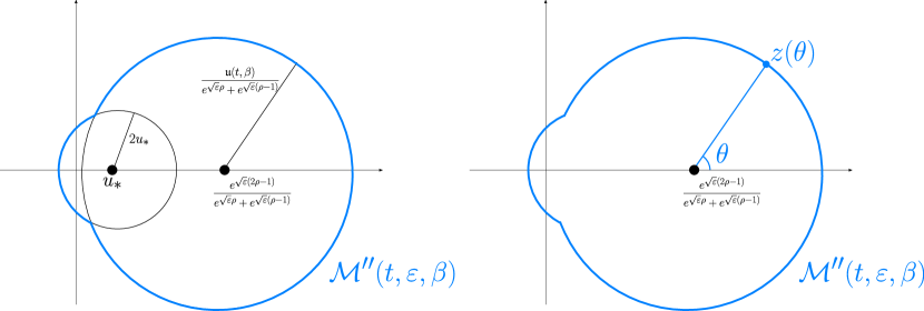
Figure 13. The contour $\mathcal{M}^{\prime\prime}(t,\varepsilon,\beta)$ and its parametrization.

We now define the $z_{1}$-contour

$$\Gamma(t,\varepsilon):=\mathcal{M}^{\prime\prime}(t,\varepsilon,-k_{1}\alpha).$$

As for the $z_{2}$-contour, we fix $k_{2}:=1$ in (6.17). Recall the definition of $\widetilde{r}_{2}(z_{1})$ from (6.18), we parametrize $z_{2}(\theta):=\widetilde{r}_{2}(z_{1})e^{\mathbf{i}\theta_{2}}\in\mathcal{C}_{\widetilde{r}_{2}(z_{1})}$.

The auxiliary parameter $k_{1}=k_{1}(\alpha)\in\mathbb{Z}_{\geq 2}$ is in place for technical purpose. We delay specifying $k_{1}$, and first explain the contour deformation we need here. Similar to the $(--)$-case, here we need a re-deformation $\mathcal{M}^{\prime\prime}(t,\varepsilon,-k_{1}\alpha)\mapsto\mathcal{N}(t,\varepsilon,-k_{1}\alpha)$ for $\mathbf{V}_{\text{res}}$. As explained earlier, the analysis of $\mathbf{V}_{\text{res}}$ favors the contour $\mathcal{N}(t,\varepsilon,-k_{1}\alpha)$. Unfortunately, we could not have chosen $\Gamma(t,\varepsilon)$ to be $\mathcal{N}(t,\varepsilon,-k_{1}\alpha)$ in the first place, because the bulk part $\mathbf{V}_{\text{blk}}$ is sensitive to crossing $z_{1}=0$ (due to the pole at $\mathfrak{p}_{\varepsilon}(z_{1})=z_{2}$). On the other hand, $\mathbf{V}_{\text{res}}$ is not. We utilize this fact to deliver the desired contour to $\mathbf{V}_{\text{res}}$ via re-deformation. Let us verify that re-deformation for $\mathbf{V}_{\text{res}}$ does not cross a pole.

Lemma 6.8.

For all $t>0$ large enough and $\varepsilon>0$ small enough, we have $\mathbf{V}_{\text{res}}=\mathbf{V}_{\text{res}}^{\prime}$, where

$$\mathbf{V}_{\text{res}}^{\prime\prime}:=\oint_{\mathcal{N}(t,\varepsilon,-k_{1}\alpha)}\mathbf{1}_{{\{|\mathfrak{p}_{\varepsilon}(z_{1})|>r^{\prime}_{2}\}}}\big{(}e^{\sqrt{\varepsilon}(\rho-1)}+e^{\sqrt{\varepsilon}\rho}\big{)}\mathfrak{J}(z_{1})\frac{\mathfrak{H}_{\varepsilon}(t,z_{1})dz_{1}}{2\pi\mathbf{i}z_{1}\mathfrak{p}_{\varepsilon}(z_{1})}$$ (6.43)

is the same as $\mathbf{V}_{\text{res}}$ except the $z_{1}$-contour is replaced by $\mathcal{N}(t,\varepsilon,-k_{1}\alpha)$.

Proof.

Referring to the definitions (6.41)–(6.42) of $\mathcal{N}(t,\varepsilon,-k_{1}\alpha)$ and $\mathcal{M}^{\prime\prime}(t,\varepsilon,-k_{1}\alpha)$ (see also Figure 13), we see that the difference $\mathcal{N}(t,\varepsilon,-k_{1}\alpha)-\mathcal{M}^{\prime\prime}(t,\varepsilon,-k_{1}\alpha)$ is the boundary of the crescent

$$\mathcal{G}(t,\varepsilon):=\big{\{}z\in\mathbb{C}:|z-u_{*}|\leq 2u_{*}\big{\}}\setminus\Big{\{}\Big{|}z-\frac{e^{\sqrt{\varepsilon}(2\rho-1)}}{e^{\sqrt{\varepsilon}\rho}+e^{\sqrt{\varepsilon}(\rho-1)}}\Big{|}\leq\frac{\mathfrak{u}(t,-k_{1}\alpha)}{e^{\sqrt{\varepsilon}\rho}+e^{\sqrt{\varepsilon}(\rho-1)}}\Big{\}}.$$

See Figure 14. With $\partial\mathcal{G}(t,\varepsilon)$ denoting the boundary, counterclockwise oriented, we have

$$\mathbf{V}_{\text{res}}-\mathbf{V}_{\text{res}}^{\prime\prime}=\frac{e^{\sqrt{\varepsilon}(\rho-1)}+e^{\sqrt{\varepsilon}\rho}}{2\pi\mathbf{i}}\oint_{\partial\mathcal{G}(t,\varepsilon)}\mathbf{1}_{{\{|\mathfrak{p}_{\varepsilon}(z_{1})|>r^{\prime}_{2}\}}}\mathfrak{J}(z_{1})\frac{1}{z_{1}\mathfrak{p}_{\varepsilon}(z_{1})}\mathfrak{H}_{\varepsilon}(t,z_{1})dz_{1}.$$

Recall that $\mathfrak{p}_{*}(z)=2-z^{-1}$ denotes the $\varepsilon\to 0$ limit of $\mathfrak{p}_{\varepsilon}$. Since $\mathcal{G}(t,\varepsilon)\subset\{|z|\leq 3u_{*}\}$ and $u_{*}<\frac{1}{12}$, on $\mathcal{G}(t,\varepsilon)$ we have $|\mathfrak{p}_{*}(z)|\geq|z|^{-1}-2\geq 2$. Consequently, $|\mathfrak{p}_{\varepsilon}(z)|>r^{\prime}_{2}$, $z\in z\in\mathcal{G}(t,\varepsilon)$, for all $t>0$ large enough and $\varepsilon>0$ small enough. We hence drop the indicator $\mathbf{1}_{{\{|\mathfrak{p}_{\varepsilon}(z_{1})|>r^{\prime}_{2}\}}}$ and write

$$\mathbf{V}_{\text{res}}-\mathbf{V}_{\text{res}}^{\prime\prime}=\frac{e^{\sqrt{\varepsilon}(\rho-1)}+e^{\sqrt{\varepsilon}\rho}}{2\pi\mathbf{i}}\oint_{\partial\mathcal{G}(t)}\frac{\mathfrak{J}(z_{1})}{z_{1}\mathfrak{p}_{\varepsilon}(z_{1})}\mathfrak{H}_{\varepsilon}(t,z_{1})dz_{1}.$$

Figure 14. The region $\mathcal{G}(t,\varepsilon)$.

It suffices to check that the integrand $\frac{\mathfrak{J}(z_{1})}{z_{1}\mathfrak{p}_{\varepsilon}(z_{1})}\mathfrak{H}_{\varepsilon}(t,z_{1})$ has no poles within $z_{1}\mathcal{G}(t,\varepsilon)$. This was carried out in the proof of Lemma 6.7 already. There we found that the $\varepsilon\to 0$ limit of the poles occurs at $\frac{1}{2}$, $b_{1}$, and $2-b_{1}$. With $u_{*}<\frac{1}{12}\wedge b_{1}$, these points sit strictly outside of $\mathcal{G}(t,\varepsilon)$ for all $t>0$ large enough and $\varepsilon>0$ small enough. Hence, no poles of $\frac{\mathfrak{J}(z_{1})}{z_{1}\mathfrak{p}_{\varepsilon}(z_{1})}\mathfrak{H}_{\varepsilon}(t,z_{1})$ enters $\mathcal{G}(t,\varepsilon)$, as long as $t>0$ is large enough and $\varepsilon>0$ is small enough. ∎

Having introduce the contours $\mathcal{M}^{\prime\prime}(t,\varepsilon,-k_{1}\alpha)$ and $\mathcal{N}(t,\varepsilon,-k_{1}\alpha)$, hereafter we write $z_{1}(\theta_{1})\in\mathcal{M}^{\prime\prime}(t,\varepsilon,-k_{1}\alpha)$ for the parametrization depicted in Figure 13, and write $\widetilde{z}_{1}(\theta_{1})\in\mathcal{N}(t,\varepsilon,-k_{1}\alpha)$ for the parametrization give in (6.41). We now turn to the auxiliary parameter $k_{1}=k_{1}(\alpha)\in\mathbb{Z}_{\geq 2}$. Similar to previous cases, the parameter $k_{1}$ is chosen large enough to ensure that

$$r^{\prime}_{2}=\mathfrak{u}(-2\alpha)\geq\mathfrak{p}_{\varepsilon}(\widetilde{z}_{1}(0))+\tfrac{1}{\sqrt{t+1}}\in\mathbb{R}.$$

Such a condition holds for a large enough $k_{1}=k_{1}(\alpha,T)$, as can be checked by the same calculations by Taylor expansion as in the $(+-)$-case. We do not repeat the calculations, and fix such $k_{1}\in\mathbb{Z}_{\geq 2}$. Given this condition, using the same argument for obtaining (6.30) in the $(+-)$-case, here we have

$$|\mathfrak{p}_{\varepsilon}(\widetilde{z}_{1}(\theta_{1}))|>r^{\prime}_{2}\text{ holds only if }|\theta_{1}|\geq\frac{1}{C(\alpha)(t+1)^{1/4}}.$$ (6.30”)

Let us check that, along the contours $z_{1}\in\mathcal{M}^{\prime\prime}(t,\varepsilon,-k_{1}\alpha)$ and $z_{1}\in\mathcal{N}(t,-k\alpha)$, and we do have the desired Gaussian decay of $|\mathfrak{D}_{\varepsilon}|$ and $|\mathfrak{H}_{\varepsilon}|$.

Lemma 6.9.

Given any $T\in(0,\infty)$ and $\beta\in\mathbb{R}$,

$$\big{|}\mathfrak{D}_{\varepsilon}(t,z)\big{|},\ \big{|}\mathfrak{H}_{\varepsilon}(t,z)\big{|}\leq C(\beta,T)\exp(-\tfrac{\theta^{2}}{C}(t+1)),\quad z=z(\theta)\in\mathcal{M}^{\prime\prime}(t,\varepsilon,\beta),$$

$$\big{|}\mathfrak{D}_{\varepsilon}(t,z)\big{|},\ \big{|}\mathfrak{H}_{\varepsilon}(t,z)\big{|}\leq C(\beta,T)\exp(-\tfrac{\theta^{2}}{C}(t+1)),\quad z=z(\theta)\in\mathcal{N}(t,\varepsilon,\beta),$$

for all $\theta\in(-\pi,\pi]$, large enough $t\leq\varepsilon^{-2}T$, and small enough $\varepsilon>0$.

Proof.

The proof follows the same three-step procedure as the proof of Lemma 6.3. Given the identities (6.9a)–(6.9c), the proof of the first two steps (Zero $\theta$)–(Small $\theta$) follows the same argument via Taylor expansion as in Lemma 6.3, and we do not repeat it here. As for the last step (Large $\theta$), as argued in the proof of Lemma 6.6, it amounts to checking the corresponding limiting condition. Recall that $\mathcal{M}=\{|z-\frac{1}{2}|=\frac{1}{2}\}$ and recall the definition of $\mathcal{M}^{\prime\prime}$ from (6.27). It is readily checked that $\mathcal{M}^{\prime\prime}(t,\varepsilon,\beta)$ converges uniformly to $\mathcal{M}^{\prime\prime}$ as $(t,\varepsilon)\to(\infty,0)$, under their respective polar parametrization, and similarly $\mathcal{N}(t,\varepsilon,\beta)$ converges uniformly to $\mathcal{M}$ as $(t,\varepsilon)\to(\infty,0)$. This being the case, the proof reduces to checking the steepest decent condition (SD.$\mathcal{M}$) and (SD.$\mathcal{M}^{\prime\prime}$), which have been verified. ∎

We have all the necessary ingredients for estimating $\mathbf{V}^{\text{in}}_{\varepsilon}$.

Proof of Proposition 6.2(c)–(d), the $(++)$-case, with large enough $t$.

The proof begins with the contour deformation described in Section 6.2. The condition (No Pole) is checked by the same argument in the $(+-)$-case, which gives the decomposition $\mathbf{V}^{\text{in}}_{\varepsilon}=\mathbf{V}_{\text{blk}}+\mathbf{V}_{\text{res}}$. We next perform the aforementioned re-deformation $\mathcal{M}^{\prime\prime}(t,\varepsilon,-k_{1}\alpha)\mapsto\mathcal{N}(t,\varepsilon,-k_{1}\alpha)$ in $\mathbf{V}_{\text{res}}$. Lemma 6.8 ensures that no pole is crossed during this step, giving $\mathbf{V}^{\text{in}}_{\varepsilon}=\mathbf{V}_{\text{blk}}+\mathbf{V}_{\text{res}}^{\prime\prime}$.

The proof amounts to bounding $\mathbf{V}_{\text{blk}}$, $\mathbf{V}_{\text{res}}^{\prime\prime}$, and their gradients. We begin with $\mathbf{V}_{\text{blk}}$. In the following we check a sequence of bounds on terms involved in (6.21), and we always assume $z_{1}=z_{1}(\theta_{1})\in\mathcal{M}^{\prime\prime}(t,\varepsilon,-k_{1}\alpha)$ and $z_{2}=z_{1}(\theta_{2})\in\mathcal{C}_{\widetilde{r}_{2}(z_{1})}$ in the course of doing so.

• Show that $|z_{1}|^{x_{2}-y_{1}+\mu_{\varepsilon}t-\lfloor\mu_{\varepsilon}t\rfloor}\leq\exp(-\frac{\alpha|x_{2}-y_{1}|}{\sqrt{t+1}+C(\alpha)})$:
  With $x_{2}-y_{1}>0$ under current assumptions, we need an upper bound on $|z_{1}|$. To this end, instead of $z_{1}\in\mathcal{M}^{\prime\prime}(t,\varepsilon,-k_{1}\alpha)$, let us first consider $\widetilde{z}_{1}\in\mathcal{N}(t,\varepsilon,-k_{1}\alpha)$. This contour $\mathcal{N}(t,\varepsilon,-k_{1}\alpha)$ is a circle with a center in $(0,\infty)$. For such circles, the farthest point to the origin occurs at the right-end. This gives

  $$\sup_{\widetilde{z}_{1}(\theta_{1})\in\mathcal{N}(t,\varepsilon,-k_{1}\alpha)}|\widetilde{z}_{1}(\theta_{1})|=\widetilde{z}_{1}(0)=\frac{e^{\sqrt{\varepsilon}(2\rho-1)}+\mathfrak{u}(t,-k_{1}\alpha)}{e^{\sqrt{\varepsilon}\rho}+e^{\sqrt{\varepsilon}(\rho-1)}}.$$

  Recall from Definition 6.5 the announced convention on Taylor expansion, and expand the last expression in $(\sqrt{\varepsilon},\frac{1}{\sqrt{t+1}})$ up to the leading order in $\frac{1}{\sqrt{t+1}}$. This gives

  $$\sup_{\widetilde{z}_{\in}\mathcal{N}(t,\varepsilon,-k_{1}\alpha)}|\widetilde{z}_{1}|=1+0\cdot\sqrt{\varepsilon}-\tfrac{1}{2}\rho(1-\rho)\varepsilon-\frac{k_{1}\alpha}{\sqrt{t+1}}+\ldots,$$

  With $k_{1}\geq 2$, and $\varepsilon\leq\frac{C(T)}{\sqrt{t+1}}$ under current assumptions, we have

  $$\sup_{\widetilde{z}_{1}\in\mathcal{N}(t,\varepsilon,-k_{1}\alpha)}|\widetilde{z}_{1}|\leq\mathfrak{u}(t,-\alpha),$$ (6.44)

  for all large enough $t$.

  Now, recall from (6.42) that $\mathcal{M}^{\prime\prime}(t,\varepsilon,-k_{1}\alpha)$ differs from $\mathcal{N}(t,\varepsilon,-k_{1}\alpha)$ only in $\{|z-u_{*}|\leq 2u_{*}\}\subset\{|z|\leq 3u_{*}\}$. With $3u_{*}<1$, the bound (6.44) readily implies

  $$\sup_{z_{1}(\theta_{1})\in\mathcal{M}^{\prime\prime}(t,\varepsilon,-k_{1}\alpha)}|\widetilde{z}_{1}(\theta_{1})|\leq\mathfrak{u}(t,-\alpha)\vee(3u_{*})=\mathfrak{u}(t,-\alpha),$$

  for all $t$ large enough. Consequently, $|z_{1}|^{x_{2}-y_{1}+\mu_{\varepsilon}t-\lfloor\mu_{\varepsilon}t\rfloor}\leq\mathfrak{u}(t,-\alpha)^{|x_{2}-y_{1}|}\leq\exp(-\frac{\alpha|x_{2}-y_{1}|}{\sqrt{t+1}+C(\alpha)}).$

• Show that $|z_{2}|^{x_{1}-y_{2}+\mu_{\varepsilon}t-\lfloor\mu_{\varepsilon}t\rfloor}\leq C(\alpha)\exp(-\frac{\alpha|x_{1}-y_{2}|}{\sqrt{t+1}+C(\alpha)})$:
  With $k_{2}:=1$ and with $\widetilde{r}_{2}$ defined in (6.18), we have $|z_{2}|\leq\mathfrak{u}(t,-\alpha)$. This and the assumption $x_{1}-y_{2}>0$ gives the desired claim.

• Show that $|\mathfrak{F}_{\varepsilon}(z_{1},z_{2})|\leq C(\alpha)(1+|\theta_{1}-\theta_{2}|\sqrt{t+1})$:
  This bound is establish by the same argument as in the $(+-)$-case. We do not repeat it here.

• Show that $|\mathfrak{D}_{\varepsilon}(z_{i})|\leq C(\alpha,T)\exp(-\frac{\theta^{2}_{i}}{C}(t+1))$:
  This is the content of Lemma 6.9.

Given ($\mathbf{V}_{\text{blk}}$.$z_{1}$)–($\mathbf{V}_{\text{blk}}$.$\mathfrak{D}_{\varepsilon}$), the desired bound on $\mathbf{V}_{\text{blk}}$ follows by inserting the bounds into (6.21), and integrating the result. The procedure is the same as the $(+-)$-case, and we do not repeat it here.

We now turn to $\mathbf{V}_{\text{res}}^{\prime\prime}$. In the following we always assume $\widetilde{z}_{1}=\widetilde{z}_{1}(\theta_{1})\in\mathcal{N}(t,\varepsilon,-k_{1}\alpha)$.

• Show that $\frac{1}{|\mathfrak{p}_{\varepsilon}(\widetilde{z}_{1})\widetilde{z}_{1}|}\leq C(\alpha)$:
  This is true because $|\mathfrak{p}_{\varepsilon}(\widetilde{z}_{1})\widetilde{z}_{1}|=\mathfrak{u}(t,-k_{1}\alpha)$.

• Show that $|\mathfrak{J}(\widetilde{z}_{1})|\leq C(\alpha)\exp(-\frac{\alpha(|x_{2}-y_{1}|+|x_{1}-y_{2}|)}{\sqrt{t+1}+C(\alpha)})$:
  Set $n_{1}:=|x_{2}-y_{1}|$ and $n_{2}:=|x_{1}-y_{2}|$. The assumption $y_{1}<y_{2}$, $x_{1}<x_{2}$ in the $(++)$-case yields $n_{1}-2\geq n_{2}>0$. Given this, recalling the definition of $\mathfrak{J}$ from (6.20), we write

  $$|\mathfrak{J}(\widetilde{z}_{1})|\leq(|\widetilde{z}_{1}|^{n_{1}-n_{2}-2}+|\widetilde{z}_{1}|^{n_{1}-n_{2}})|\widetilde{z}_{1}\mathfrak{p}_{\varepsilon}(\widetilde{z}_{1}))|^{n_{2}}.$$

  Given the bound (6.44) on $|\widetilde{z}_{1}|$ and given that $|\mathfrak{p}_{\varepsilon}(\widetilde{z}_{1})\widetilde{z}_{1}|=\mathfrak{u}(t,-k_{1}\alpha)$, we have

  $$|\mathfrak{J}(\widetilde{z}_{1})|\leq 2\mathfrak{u}(t,-\alpha)^{n_{1}-n_{2}-2}\mathfrak{u}(t,-k_{1}\alpha)^{n_{2}}.$$

  With $k_{1}\geq 2$, the desired result follows:

  $$|\mathfrak{J}(\widetilde{z}_{1})|\leq C(\alpha)e^{\frac{-\alpha(n_{1}-n_{2})}{\sqrt{t+1}+C(\alpha)}}e^{-\frac{2\alpha n_{2}}{\sqrt{t+1}+C(\alpha)}}=C(\alpha)e^{-\frac{\alpha(n_{1}+n_{2})}{\sqrt{t+1}+C(\alpha)}}.$$

• Show that $|\mathfrak{H}_{\varepsilon}(\widetilde{z}_{1})|\leq C(\alpha,T)\exp(-\frac{\theta^{2}_{1}}{C}(t+1))$:
  This is the content of Lemma 6.9.

Given ($\mathbf{V}_{\text{res}}^{\prime\prime}$.$\frac{1}{z_{1}\mathfrak{p}_{\varepsilon}}$)–($\mathbf{V}_{\text{res}}^{\prime\prime}$.$\mathfrak{H}_{\varepsilon}$), and the derived constraint (6.30”) on $|\theta_{1}|$, the desired bound on $\mathbf{V}_{\text{res}}$ follows the same integration procedure is the same as the $(+-)$-case.

As for the gradient, similarly to the $(+-)$-case, here we have

$$|z_{j}^{\pm}-1|\leq\tfrac{1}{\sqrt{t+1}}+|\theta_{j}|,\ z_{1}=z_{1}(\theta)\in\mathcal{M}^{\prime\prime}(t,\varepsilon,-k_{1}\alpha)\text{ or }\mathcal{N}(t,\varepsilon,-k_{1}\alpha),\ z_{2}=z_{2}(\theta)\in\mathcal{C}_{\widetilde{r}_{2}(z_{1})}.$$ (6.33”)

Incorporate this bound into the preceding analysis gives the desired bounds on the gradients. ∎

7. Controlling the quadratic variation: Proof of Proposition 5.6

Based on the estimates from Section 6 and the duality of the stochastic 6V model from Section 3, here we prove Proposition 5.6.

7.1. Expanding the quadratic variation

The first step toward proving Proposition 5.6 is to find an expression for $\varepsilon^{-1}\Theta_{1}(t,x)\Theta_{2}(t,x)$ that exposes the limiting behavior $\frac{2b_{1}\rho(1-\rho)}{1+b_{1}}Z^{2}(t,x)$. Recall the definition of $\Theta_{1}(t,x)$ and $\Theta_{2}(t,x)$ from (4.20)–(4.21). With $\sum_{i=0}^{\infty}\mathsf{p}_{\varepsilon}(i-\mu)=1$, we rewrite them as

$$\varepsilon^{-\frac{1}{2}}\Theta_{1}(t,x) =\varepsilon^{-\frac{1}{2}}(\lambda_{\varepsilon}\tau_{\varepsilon}^{-1}-1)Z(t,x)-\varepsilon^{-\frac{1}{2}}\sum_{i=0}^{\infty}\mathsf{p}_{\varepsilon}(i-\mu)\big{(}Z(t,x-i)-Z(t,x)\big{)},$$ (7.1)

$$\varepsilon^{-\frac{1}{2}}\Theta_{2}(t,x) =\varepsilon^{-\frac{1}{2}}(1-\lambda_{\varepsilon})Z(t,x)+\varepsilon^{-\frac{1}{2}}\sum_{i=0}^{\infty}\mathsf{p}_{\varepsilon}(i-\mu)\big{(}Z(t,x-i)-Z(t,x)\big{)}.$$ (7.2)

In order the extract the relevant limiting behaviors, in the sequel we will perform a sequence of expansions on the r.h.s. of (7.1)–(7.2). Here, let us prepare some notation to express various error terms throughout the subsequent expansions. We use $\mathcal{G}_{\varepsilon}(t,x_{1},\ldots,x_{n};x)$ to denote a generic (random) process that has a uniform exponential decay off the point $x$; and use $\mathcal{B}_{\varepsilon}(t,x_{1},\ldots,x_{n})$ to denote a generic uniformly bounded (random) process. More precisely, there exists deterministic $a>0$, $C<\infty$ such that, for all $\varepsilon\in(0,1)$, $t\in\mathbb{Z}_{\geq 0}$ , $x_{1},\ldots,x_{n},x\in\Xi(t)$,

$$|\mathcal{G}_{\varepsilon}(t,x_{1},\ldots,x_{n};x)| \leq C\exp(-a|x_{1}-x|-\ldots-a|x_{1}-x|),$$

$$|\mathcal{B}_{\varepsilon}(t,x_{1},\ldots,x_{n})| \leq C.$$

With these notation we write $\mathcal{X}_{\text{bdd}}(t,x)$ for a generic expression of the form

$$\mathcal{X}_{\text{bdd}}(t,x)=\sum_{x_{1},x_{2}\in\Xi(t)}\mathcal{G}_{\varepsilon}(t,x_{1},x_{2};x)Z(t,x_{1})Z(t,x_{2}),$$ (7.3)

where ‘bdd’ stands for ‘bounded’. In the sequel $\mathcal{G}_{\varepsilon}$, $\mathcal{B}_{\varepsilon}$ and $\mathcal{X}_{\text{bdd}}$ may differ from line to line, as they refer to generic expressions of the declared type. Under this notation, we view expression of the type $\varepsilon^{u}\mathcal{X}_{\text{bdd}}(t,x)$, $u>0$, small and negligible.

We will also consider expressions that involve gradients. To motivate the definitions of the following expressions, let us first consider an expansion of $\nabla Z(t,x)$. Recall that $\nabla f(x):=f(x+1)-f(x)$ denotes the (forward) discrete gradient, and recall from (4.24) that $\eta_{\text{c}}(t,x)\in\{0,1\}$, $x\in\Xi(t)$, denote the centered occupation variable. Referring back to the definition (4.6) of $Z$, with $\tau_{\varepsilon}=\exp(-\sqrt{\varepsilon})$, we see that $\nabla Z(t,x)=(e^{-\sqrt{\varepsilon}(\eta_{\text{c}}^{+}(t,x)-\rho)}-1)Z(t,x).$ Taylor expanding the exponential gives

$$\varepsilon^{-\frac{1}{2}}\nabla Z(t,x) =-\big{(}\eta_{\text{c}}^{+}Z\big{)}(t,x)+\rho Z(t,x)+\sqrt{\varepsilon}\mathcal{B}_{\varepsilon}(t,x)Z(t,x),$$ (7.4)

In particular,

$$\varepsilon^{-\frac{1}{2}}\nabla Z(t,x)=\mathcal{B}_{\varepsilon}(t,x)Z(t,x).$$ (7.5)

Such a bound (7.5) is pointwise. As it turn out, after a suitable time averaging, expressions that involves $\varepsilon^{-\frac{1}{2}}\nabla$ acting on $Z$ decay to zero (except for a product of two $\varepsilon^{-\frac{1}{2}}\nabla Z$ evaluated at the same site, see (7.8) and Lemma 7.1 below). The underlying mechanism arises from the structure for the semigroup $\mathbf{V}_{\varepsilon}$: referring to Proposition 6.1, we see that $\mathbf{V}_{\varepsilon}$ gains an extra factor $(t+1)^{-\frac{1}{2}}$ upon taking gradient. This being the case, we view expressions of the type

$$Z_{\nabla}(t,x_{1},x_{2}):=(\varepsilon^{-\frac{1}{2}}\nabla Z(t,x_{1}))Z(t,x_{2})$$

as small, and consider generic linear combinations of them

$$\mathcal{Y}_{\nabla}(t,x) =\sum_{x_{1},x_{2}\in\Xi(t)}\gamma_{\varepsilon}(t,x_{1},x_{2};x)Z_{\nabla}(t,x_{1},x_{2}),$$ (7.6)

with some deterministic coefficients $\gamma_{\varepsilon}(t,x_{1},x_{2};x)$ that decay exponentially off $x$:

$$|\gamma_{\varepsilon}(t,x_{1},x_{2};x)|\leq C\exp(-a|x_{1}-x|-a|x_{2}-x|).$$ (7.7)

We will also consider generic expressions that involves two pieces of gradient:

$$\mathcal{Y}_{\nabla,\nabla}(t,x)=\sum_{x_{1}<x_{2}\in\Xi(t)}\gamma_{\varepsilon}(t,x_{1},x_{2};x)(\varepsilon^{-\frac{1}{2}}\nabla Z)(t,x_{1})(\varepsilon^{-\frac{1}{2}}\nabla Z)(t,x_{2}),$$ (7.8)

for some generic deterministic coefficients $\gamma_{\varepsilon}(t,x_{1},x_{2};x)$ satisfying (7.7), (and may differ from line to line in the sequel).

Note that in (7.8), the sum ranges over distinct $x_{1}$ and $x_{2}$. In fact, diagonal terms $x_{1}=x_{2}$ contains non-negligible contributions:

Lemma 7.1.

We have that

$$(\varepsilon^{-\frac{1}{2}}\nabla Z)^{2}(t,x)-\rho(1-\rho)Z^{2}(t,x)=-Z_{\nabla}(t,x,x+1)+\varepsilon^{\frac{1}{2}}\mathcal{B}_{\varepsilon}(t,x)Z^{2}(t,x).$$

Proof.

To expose the relevant contribution from this expression, we appeal the expansion (7.4) of $\varepsilon^{-\frac{1}{2}}\nabla Z$, square it, followed by using $\eta_{\text{c}}^{2}=\eta_{\text{c}}$. This gives (recall $\eta_{\text{c}}$ from (4.24))

$$( \varepsilon^{-\frac{1}{2}}\nabla Z(t,x))^{2}=\Big{(}-\eta_{\text{c}}(t,x+1)Z(t,x)+\rho Z(t,x)+\varepsilon^{\frac{1}{2}}\mathcal{B}_{\varepsilon}(t,x)Z(t,x)\Big{)}^{2}$$

$$=\Big{(}\eta_{\text{c}}(t,x+1)Z^{2}(t,x)-2\rho\eta_{\text{c}}(t,x+1)Z^{2}(t,x)+\rho^{2}Z^{2}(t,x)\Big{)}+\varepsilon^{\frac{1}{2}}\big{(}\mathcal{B}_{\varepsilon}(t,x)Z^{2}(t,x)\big{)}$$

$$=\Big{(}\big{(}(1-2\rho)\eta_{\text{c}}^{+}Z^{2}+\rho^{2}Z^{2}\big{)}+\varepsilon^{\frac{1}{2}}\mathcal{B}_{\varepsilon}Z^{2}\Big{)}\Big{|}_{x}.$$

Use (7.4) in reverse: $\eta_{\text{c}}^{+}Z=-\varepsilon^{-\frac{1}{2}}\nabla Z+\rho Z+\varepsilon^{\frac{1}{2}}\mathcal{B}_{\varepsilon}Z$, we rewrite the expression $\eta_{\text{c}}^{+}Z^{2}$ as $-(\varepsilon^{-\frac{1}{2}}\nabla Z)Z+\rho Z^{2}+\varepsilon^{\frac{1}{2}}\mathcal{B}_{\varepsilon}Z^{2}$. Inserting this into the last displayed equation gives the desired result. ∎

Having introduced the necessary notation and tools, we now begin to expand $\Theta_{1}$ and $\Theta_{2}$.

Lemma 7.2.

We have that

$$\varepsilon^{-1}\Theta_{1}(t,x)\Theta_{2}(t,x)-\tfrac{2b_{1}\rho(1-\rho)}{1+b_{1}} Z^{2}(t,x)=\sqrt{\varepsilon}\mathcal{X}_{\text{bdd}}(t,x)+\mathcal{Y}_{\nabla}(t,x)+\mathcal{Y}_{\nabla,\nabla}(t,x).$$

Proof.

The starting point of the proof is the expressions (7.1)–(7.2) for $\Theta_{1}(t,x)$ and $\Theta_{2}(t,x)$. First, from (1.3) and $\tau_{\varepsilon}^{-1}=e^{\sqrt{\varepsilon}}$, we have that $\varepsilon^{-\frac{1}{2}}(\lambda_{\varepsilon}\tau_{\varepsilon}^{-1}-1)=(1-\rho)+\mathcal{O}(\varepsilon^{\frac{1}{2}})$ and that $\varepsilon^{-\frac{1}{2}}(1-\lambda_{\varepsilon})=\rho+\mathcal{O}(\varepsilon^{\frac{1}{2}})$. Given this, in (7.1)–(7.2) we replace $\varepsilon^{-\frac{1}{2}}(\lambda_{\varepsilon}\tau_{\varepsilon}^{-1}-1)$ with $(1-\rho)$ and replace $\varepsilon^{-\frac{1}{2}}(1-\lambda_{\varepsilon})$ with $\rho$, up to errors of the form $\varepsilon^{\frac{1}{2}}\mathcal{B}_{\varepsilon}(t,x)$. Further, telescope the expression $Z(t,x-i)-Z(t,x)$ into $-\nabla Z(t,x-i)-\nabla Z(t,x-i+1)-\ldots-\nabla Z(t,x-1)$. This, combined with (1.3), gives

$$\varepsilon^{-\frac{1}{2}}\Theta_{1}(t,x) =(1-\rho)Z(t,x)+\sum_{i=0}^{\infty}\sum_{0<j\leq i}\mathsf{p}_{\varepsilon}(i-\mu_{\varepsilon})\varepsilon^{-\frac{1}{2}}\nabla Z(t,x-j)+\varepsilon^{\frac{1}{2}}\mathcal{B}_{\varepsilon}(t,x)Z(t,x),$$

$$\varepsilon^{-\frac{1}{2}}\Theta_{2}(t,x) =\rho Z(t,x)-\sum_{i=0}^{\infty}\sum_{0<j\leq i}\mathsf{p}_{\varepsilon}(i-\mu_{\varepsilon})\varepsilon^{-\frac{1}{2}}\nabla Z(t,x-j)+\varepsilon^{\frac{1}{2}}\mathcal{B}_{\varepsilon}(t,x)Z(t,x).$$

To simplify notation, set $u_{\varepsilon}(j):=\sum_{i=j}^{\infty}\mathsf{p}_{\varepsilon}(i-\mu_{\varepsilon})$, we write

$$\varepsilon^{-\frac{1}{2}}\Theta_{1}(t,x) =(1-\rho)Z(t,x)+\sum_{j=1}^{\infty}u_{\varepsilon}(j)\varepsilon^{-\frac{1}{2}}\nabla Z(t,x-j)+\varepsilon^{\frac{1}{2}}\mathcal{B}_{\varepsilon}(t,x)Z(t,x).$$ (7.9)

$$\varepsilon^{-\frac{1}{2}}\Theta_{2}(t,x) =\rho Z(t,x)-\sum_{j=1}^{\infty}u_{\varepsilon}(j)\varepsilon^{-\frac{1}{2}}\nabla Z(t,x-j)+\varepsilon^{\frac{1}{2}}\mathcal{B}_{\varepsilon}(t,x)Z(t,x).$$ (7.10)

The next step is to take the product of (7.9)–(7.10). Let $A_{1,Z},A_{1,\nabla},A_{1,\text{err}}$ denote the respective terms on the r.h.s. of (7.9), and similarly $A_{2,Z},A_{2,\nabla},A_{2,\text{err}}$ for (7.10). In the following we expand

$$\varepsilon^{-1}\Theta_{1}(t,x)\Theta_{2}(t,x)=\big{(}A_{1,Z}+A_{1,\nabla}+A_{1,\text{err}}\big{)}\big{(}A_{2,Z}+A_{2,\nabla}+A_{2,\text{err}}\big{)},$$

and analyze the resulting terms.

• Indeed, $A_{1,Z}A_{2,Z}=\rho(1-\rho)Z^{2}(t,x)$.

• Next, the term $A_{1,Z}A_{2,\nabla}+A_{1,\nabla}A_{2,Z}$.

  Indeed $A_{1,Z}A_{2,\nabla}+A_{1,\nabla}A_{2,Z}$ is a linear combination of $Z(t,x)\varepsilon^{-\frac{1}{2}}\nabla Z(t,x-j)$, with coefficients $(2\rho-1)u_{\varepsilon}(j)$. Let us check that $u_{\varepsilon}(j)$ decays exponentially in $|j|$. Referring back to (4.11), with $\mu_{\varepsilon},\lambda_{\varepsilon}\to 1$ as $\varepsilon\to 0$, the kernel $\mathsf{p}_{\varepsilon}$ decays geometrically, uniformly over $\varepsilon\in(0,1)$:

  $$\mathsf{p}_{\varepsilon}(x)\leq Cb_{1}^{-|x|}.$$ (7.11)

  From this we see that

  $$|u_{\varepsilon}(j)|=\sum_{i\in\mathbb{Z}_{\geq j}}\mathsf{p}_{\varepsilon}(i-\mu_{\varepsilon})\leq C|j|b_{1}^{|j|}\leq Ce^{-\frac{1}{2}|\log b_{1}||j|}.$$ (7.12)

  Given this property (7.12), we conclude that $A_{1,Z}A_{2,\nabla}+A_{1,\nabla}A_{2,Z}$ is a linear combination of $Z(t,x)\varepsilon^{-\frac{1}{2}}\nabla Z(t,x-j)$, with deterministic coefficients that decay exponentially in $|j|$, whereby

  $$A_{1,Z}A_{2,\nabla}+A_{1,\nabla}A_{2,Z}=\mathcal{Y}_{\nabla}(t,x).$$

• We now turn to $A_{1,\nabla}A_{2,\nabla}$.

  With $A_{1,\nabla}$ and $A_{2,\nabla}$ both being sums, in the produce of $A_{1,\nabla}A_{2,\nabla}$, we separate the diagonal and off-diagonal term. Off-diagonal terms form a linear combination of $\varepsilon^{-\frac{1}{2}}\nabla Z(x-j)\varepsilon^{-\frac{1}{2}}\nabla Z(x-j^{\prime})$, $j\neq j^{\prime}$, with coefficient $u_{\varepsilon}(j)u_{\varepsilon}(j^{\prime})$. Thanks to (7.12), this coefficient decays exponentially in $|j|+|j^{\prime}|$. This being the case, off-diagonal terms jointly contribute an expression of the type $\mathcal{Y}_{\nabla,\nabla}(t,x)$. We hence keep track of only the diagonal terms, and write

  $$A_{1,\nabla}A_{2,\nabla}=-\sum_{j=1}^{\infty}u_{\varepsilon}(j)^{2}(\nabla Z(t,x-j))^{2}+\mathcal{Y}_{\nabla,\nabla}(t,x).$$

• Lastly, everything else: $(A_{1,Z}+A_{1,\nabla})A_{2,\text{err}}+A_{1,\text{err}}(A_{2,Z}+A_{2,\nabla})+A_{1,\text{err}}A_{2,\text{err}}$.

  First, by (7.5), in $A_{i,\nabla}$ we replace each $\varepsilon^{-\frac{1}{2}}\nabla Z(t,x-j)$ with $\mathcal{B}_{\varepsilon}(t,x-j)Z(t,x-j)$. Once this is done, expanding the expression $(A_{1,Z}+A_{1,\nabla})A_{2,\text{err}}+A_{1,\text{err}}(A_{2,Z}+A_{2,\nabla})+A_{1,\text{err}}A_{2,\text{err}}$ gives

  $$\varepsilon^{\frac{1}{2}}\big{(}\ \text{linear combination of }\mathcal{B}_{\varepsilon}(t,x,x-j)\mathcal{B}_{\varepsilon}(t,x,x-j^{\prime})\ \big{)}Z(t,x)^{2}.$$

  Thanks to (7.12), the coefficients within the linear combination decays exponentially in $|j|+|j^{\prime}|$. This gives

  $$(A_{1,Z}+A_{1,\nabla})A_{2,\text{err}}+A_{1,\text{err}}(A_{2,Z}+A_{2,\nabla})+A_{1,\text{err}}A_{2,\text{err}}=\varepsilon^{\frac{1}{2}}\mathcal{X}_{\text{bdd}}(t,x).$$

Given the preceding discussion, we now have

$$\begin{split}\varepsilon^{-1}\Theta_{1}(t,x)\Theta_{2}(t,x)=&\rho(1-\rho)Z^{2}(t,x)+\sqrt{\varepsilon}\mathcal{X}_{\text{bdd}}(t,x)+\mathcal{Y}_{\nabla}(t,x)+\mathcal{Y}_{\nabla,\nabla}(t,x)\\ &-\sum_{j=1}^{\infty}u_{\varepsilon}(j)^{2}(\varepsilon^{-\frac{1}{2}}\nabla Z(t,x-j))^{2}.\end{split}$$ (7.13)

As shown in Lemma 7.1, the last term in (7.13) contains a non-negligible contribution to $Z^{2}(t,x)$. The rest of the proof consists of extracting this contribution. First, using Lemma 7.1, we write

$$\sum_{j=1}^{\infty}u_{\varepsilon}(j)^{2}(\varepsilon^{-\frac{1}{2}}\nabla Z(t,x-j))^{2}-\rho(1-\rho)A=\mathcal{Y}_{\nabla}(t,x)+\varepsilon^{\frac{1}{2}}\mathcal{X}_{\text{bdd}}(t,x),$$ (7.14)

where $A:=\sum_{j=1}^{\infty}u_{\varepsilon}(j)^{2}Z^{2}(t,x-j)$. The focus now is on the term $A$. We argue that, replacing $Z(t,x-j)$ with $Z(t,x)$ in $A$ only produces an affordable error. To see this, write

$$\big{|}Z(t,x-j)-Z(t,x)\big{|}=\big{|}e^{\sqrt{\varepsilon}\sum_{i=0}^{j-1}(\eta_{\text{c}}(t,x-i)-\rho)}-1\big{|}Z(t,x)\leq\sqrt{\varepsilon}|j|e^{\sqrt{\varepsilon}|j|}Z(t,x).$$ (7.15)

Now, write $Z(t,x-j)$ as $Z(t,x)+Z(t,x-j)-Z(t,x)$, with the aid of (7.15) and (7.12), we have

$$A=Z^{2}(t,x)\sum_{j=1}^{\infty}u^{2}_{\varepsilon}(j)+\varepsilon^{\frac{1}{2}}\mathcal{B}_{\varepsilon}(t,x)Z^{2}(t,x).$$ (7.16)

With (1.3), and $b_{2}=e^{-\sqrt{\varepsilon}}b_{1}$, a straightforward calculation from (4.11) gives

$$\sum_{j=1}^{\infty}u^{2}_{\varepsilon}(j)=\frac{1-b_{1}}{1+b_{1}}+\mathcal{O}(\sqrt{\varepsilon}).$$

Using this in (7.16), and inserting the result back into (7.14), we conclude

$$\sum_{j=1}^{\infty}u_{\varepsilon}(j)^{2}(\varepsilon^{-\frac{1}{2}}\nabla Z(t,x-j))^{2}-\rho(1-\rho)\frac{1-b_{1}}{1+b_{1}}Z^{2}(t,x)=\mathcal{Y}_{\nabla}(t,x)+\varepsilon^{\frac{1}{2}}\mathcal{X}_{\text{bdd}}(t,x).$$

This together with (7.13) gives the desired result. ∎

Lemma 7.2 provides the relevant decomposition of $\varepsilon^{-1}\Theta_{1}\Theta_{2}$ into its limiting expression and residual terms. While we do expect the residual terms $\varepsilon^{\frac{1}{2}}\mathcal{X}_{\text{bdd}}$, $\mathcal{Y}_{\nabla}$, and $\mathcal{Y}_{\nabla,\nabla}$ to tend to zero, bounds on the last two terms are not immediate. To see this, recall from Proposition 4.3 that the duality functions for the stochastic 6V model are $Z(s,x_{1})Z(s,x_{2})$ and $(\eta_{\text{c}}^{+}Z)(s,x_{1})(\eta_{\text{c}}^{+}Z)(s,x_{2})$, for $x_{1}<x_{2}$. On the other hand, the expressions $\mathcal{Y}_{\nabla}$ and $\mathcal{Y}_{\nabla,\nabla}$ (as in (7.6) and (7.8)) are linear combinations of $Z(s,x_{1})Z(s,x_{2})$. that generally involve $x_{1}=x_{2}$.

To circumvent this ‘diagonal’ issue, recalling from (7.7) that $\gamma_{\varepsilon}$ denotes generic deterministic coefficients with an exponential decay, we consider a slight modification $\mathcal{X}_{\nabla}$ of $\mathcal{Y}_{\nabla}$, which is the same type of expressions with an additional constraint $|x_{1}-x_{2}|>1$:

$$\mathcal{X}_{\nabla}(t,x)=\sum_{x_{1},x_{2}\in\Xi(t),|x_{2}-x_{1}|>1}\gamma_{\varepsilon}(t,x_{1},x_{2};x)Z_{\nabla}(s,x_{1},x_{2}).$$

Next, set

$$\widetilde{Z}(t,x_{1},x_{2}):=\big{(}\eta_{\text{c}}^{+}Z\big{)}(t,x_{1})\big{(}\eta_{\text{c}}^{+}Z\big{)}(t,x_{2})-\rho^{2}Z(t,x_{1})Z(t,x_{2}).$$ (7.17)

In place of $\mathcal{Y}_{\nabla,\nabla}$, we consider expressions $\mathcal{X}_{\widetilde{Z}}$ of the type

$$\mathcal{X}_{\widetilde{Z}}(t,x) =\sum_{x_{1}<x_{2}\in\Xi(t)}\gamma_{\varepsilon}(t,x_{1},x_{2};x)\widetilde{Z}(t,x_{1},x_{2}).$$ (7.18)

The next lemma allows us to trade in $\mathcal{Y}_{\nabla}$ and $\mathcal{Y}_{\nabla,\nabla}$ for $\mathcal{X}_{\nabla}$ and $\mathcal{X}_{\widetilde{Z}}$.

Lemma 7.3.

We have that

$$\mathcal{Y}_{\nabla,\nabla}(t,x) =\mathcal{X}_{\widetilde{Z}}(t,x)+\mathcal{Y}_{\nabla}(t,x)+\varepsilon^{\frac{1}{2}}\mathcal{X}_{\text{bdd}}(t,x),$$ (7.19)

$$\mathcal{Y}_{\nabla}(t,x) =\mathcal{X}_{\nabla}(t,x)+\varepsilon^{\frac{1}{2}}\mathcal{X}_{\text{bdd}}(t,x).$$ (7.20)

Proof.

Indeed, $\mathcal{Y}_{\nabla,\nabla}(t,x)$ denotes a generic linear combination of

$$A:=(\varepsilon^{-\frac{1}{2}}\nabla Z)(t,x_{1})(\varepsilon^{-\frac{1}{2}}\nabla Z)(t,x_{2}),\quad x_{1}<x_{2},$$

and $\mathcal{X}_{\widetilde{Z}}(t,x)$ denotes a generic linear combination of $\widetilde{Z}(t,x_{1},x_{2})$, $x_{1}<x_{2}$. This being the case, to prove (7.19), it suffices to show that $A-\widetilde{Z}(t,x_{1},x_{2})$ is written as a linear combination of $Z_{\nabla}(t,x_{1},x_{2})$ and negligible terms that carry an outstanding $\varepsilon^{\frac{1}{2}}$ factor. To this end, we use (7.4) to expand

$$A= \big{(}-\eta_{\text{c}}^{+}Z+\rho Z+\varepsilon^{\frac{1}{2}}\mathcal{B}_{\varepsilon}Z\big{)}(t,x_{1})\big{(}-\eta_{\text{c}}^{+}Z+\rho Z+\varepsilon^{\frac{1}{2}}\mathcal{B}_{\varepsilon}Z\big{)}(t,x_{2})$$

$$= \widetilde{Z}(t,x_{1},x_{2})+\rho\big{(}-\eta_{\text{c}}^{+}Z+\rho Z\big{)}(t,x_{1})Z(t,x_{2})+\rho Z(t,x_{1})\big{(}-\eta_{\text{c}}^{+}Z+\rho Z\big{)}(t,x_{2})$$ (7.21)

$$+\varepsilon^{\frac{1}{2}}\mathcal{B}_{\varepsilon}(t,x_{1},x_{2})Z(t,x_{1})Z(t,x_{2}).$$

In (7.21), further use (7.4) in reverse to write $-\eta_{\text{c}}^{+}Z+\rho Z=\varepsilon^{-\frac{1}{2}}\nabla Z+\varepsilon^{\frac{1}{2}}\mathcal{B}_{\varepsilon}Z$. We get

$$A-\widetilde{Z}(t,x_{1},x_{2})=\rho Z_{\nabla}(t,x_{1},x_{2})+\rho Z_{\nabla}(t,x_{2},x_{1})+\varepsilon^{\frac{1}{2}}\mathcal{B}_{\varepsilon}(t,x_{1},x_{2})Z(t,x_{1})Z(t,x_{2}).$$

This gives the desired result (7.19).

As for (7.20), recall that both $\mathcal{X}_{\nabla}$ and $\mathcal{Y}_{\nabla}$ denote generic linear combinations of the same terms. The only difference is in that the former misses those terms with $|x_{1}-x_{2}|\leq 1$. Consequently, the result (7.20) follows once we show

$$Z(t,x+1)\big{(}\varepsilon^{-\frac{1}{2}}\nabla Z(t,x)\big{)} =Z(t,x+2)\big{(}\varepsilon^{-\frac{1}{2}}\nabla Z(t,x)\big{)}+\varepsilon^{\frac{1}{2}}\big{(}\mathcal{B}_{\varepsilon}Z^{2}\big{)}(t,x),$$

$$Z(t,x)\big{(}\varepsilon^{-\frac{1}{2}}\nabla Z(t,x+1)\big{)} =Z(t,x-1)\big{(}\varepsilon^{-\frac{1}{2}}\nabla Z(t,x+1)\big{)}+\varepsilon^{\frac{1}{2}}\big{(}\mathcal{B}_{\varepsilon}Z^{2}\big{)}(t,x),$$

$$Z(t,x)\big{(}\varepsilon^{-\frac{1}{2}}\nabla Z(t,x)\big{)} =Z(t,x-2)\big{(}\varepsilon^{-\frac{1}{2}}\nabla Z(t,x)\big{)}+\varepsilon^{\frac{1}{2}}\big{(}\mathcal{B}_{\varepsilon}Z^{2}\big{)}(t,x).$$

Going from the l.h.s. to the r.h.s. amounts to changing $Z(t,x+1)\mapsto Z(t,x+2)$ or changing $Z(t,x)\mapsto Z(t,x-1)$; note that the $\nabla Z$ factor is never changed. Thanks to (7.4), these changes introduce only error of the form $\varepsilon^{\frac{1}{2}}(\mathcal{B}_{\varepsilon}Z)(t,x)$. Also, by (7.5), $\varepsilon^{-\frac{1}{2}}\nabla Z(t,x)=(\mathcal{B}_{\varepsilon}Z)(t,x)$, $\varepsilon^{-\frac{1}{2}}\nabla Z(t,x+1)=(\mathcal{B}_{\varepsilon}Z)(t,x)$. Hence, the overall error caused by the aforementioned changes is indeed of the form $\varepsilon^{\frac{1}{2}}(\mathcal{B}_{\varepsilon}Z^{2})(t,x)$. ∎

Lemmas 7.2 and 7.3 immediately yield

Corollary 7.4.

We have

$$\varepsilon^{-1}\Theta_{1}(t,x)\Theta_{2}(t,x)-\frac{2b_{1}\rho(1-\rho)}{1+b_{1}}Z^{2}(t,x)=\sqrt{\varepsilon}\mathcal{X}_{\text{bdd}}(t,x)+\mathcal{X}_{\nabla}(t,x)+\mathcal{X}_{\widetilde{Z}}(t,x).$$

7.2. Time decorrelation via duality

Given the decomposition from Corollary 7.4, our goal toward proving Proposition 5.6 is to argue that, each type of expression on the r.h.s. is negligible as $\varepsilon\to 0$. This is straightforward for $\sqrt{\varepsilon}\mathcal{X}_{\text{bdd}}(t,x)$ due to the outstanding $\varepsilon^{\frac{1}{2}}$ factor. On the other hand, as mentioned earlier, the terms $\mathcal{X}_{\nabla}$ and $\mathcal{X}_{\widetilde{Z}}$ converge to zero only after time averaging. This being the case, with $\mathcal{X}_{\nabla}$ and $\mathcal{X}_{\widetilde{Z}}$ being linear combinations of $Z_{\nabla}$ and $\widetilde{Z}$, we direct our focus onto bounding

$$B_{\mathcal{X}_{\nabla}}(\overline{t},x^{\star}_{1},x^{\star}_{2}) :=\mathbb{E}\Bigg{[}\Big{(}\varepsilon^{2}\sum_{s=0}^{\overline{t}-1}Z_{\nabla}(s,x^{\star}_{1}(s),x^{\star}_{2}(s))\Big{)}^{2}\Bigg{]},$$ (7.22)

$$B_{\mathcal{X}_{\widetilde{Z}}}(\overline{t},x^{\star}_{1},x^{\star}_{2}) :=\mathbb{E}\Bigg{[}\Big{(}\varepsilon^{2}\sum_{s=0}^{\overline{t}-1}\widetilde{Z}(s,x^{\star}_{1}(s),x^{\star}_{2}(s))\Big{)}^{2}\Bigg{]},$$ (7.23)

for $\overline{t}\in\mathbb{Z}\cap[0,\varepsilon^{-2}T]$ and $x^{\star}_{1}\neq x_{2}^{\star}\in\mathbb{Z}$, and $x^{\star}_{i}(s):=x^{\star}_{i}-\mu_{\varepsilon}s+\lfloor\mu_{\varepsilon}s\rfloor\in\Xi(s).$ These expressions are expanded into conditional expectations as

$$B_{\mathcal{X}_{\nabla}}(\overline{t},x^{\star}_{1},x^{\star}_{2}) =\varepsilon^{4}\Big{(}2\sum_{s_{1}<s_{2}<\overline{t}}+\sum_{s_{1}=s_{2}<\overline{t}}\Big{)}\mathbb{E}\Big{[}\mathbb{E}\big{[}Z_{\nabla}(s_{2},x_{1},x_{2})\big{|}\mathscr{F}(s_{1})\big{]}Z_{\nabla}(s_{1},x_{1},x_{2})\Big{]},$$ (7.24)

$$B_{\mathcal{X}_{\widetilde{Z}}}(\overline{t},x^{\star}_{1},x^{\star}_{2}) =\varepsilon^{4}\Big{(}2\sum_{s_{1}<s_{2}<\overline{t}}+\sum_{s_{1}=s_{2}<\overline{t}}\Big{)}\mathbb{E}\Big{[}\mathbb{E}\big{[}\widetilde{Z}(s_{2},x_{1},x_{2})\big{|}\mathscr{F}(s_{1})\big{]}\widetilde{Z}(s_{1},x_{1},x_{2})\Big{]},$$ (7.25)

where $x_{i}:=x^{\star}_{i}-\mu_{\varepsilon}s_{i}+\lfloor\mu_{\varepsilon}s_{i}\rfloor$ and the notation $(\sum+\sum)({\raisebox{-2.15277pt}{\scalebox{1.8}{$\cdot$}}}):=\sum({\raisebox{-2.15277pt}{\scalebox{1.8}{$\cdot$}}})+\sum({\raisebox{-2.15277pt}{\scalebox{1.8}{$\cdot$}}})$. Given (7.24)–(7.25), we set out to bounding the following conditional expectations

$$\mathbb{E}\big{[}(Z_{\nabla}(t+s,x_{1},x_{2})|\mathscr{F}(s)\big{]}Z_{\nabla}(s,x_{1},x_{2}),\quad\mathbb{E}\big{[}\widetilde{Z}(t+s,x_{1},x_{2})|\mathscr{F}(s)\big{]}\widetilde{Z}(s,x_{1},x_{2}),$$

and show that they decay as $t$ becomes large. We begin by relating these conditional expectations to the semigroup $\mathbf{V}_{\varepsilon}$ via duality. Recall that $\nabla_{x}$ denotes the discrete gradient acting on a designated variable $x$.

Lemma 7.5.

Let $t,s\in\mathbb{Z}_{\geq 0}$. For all $x_{1}+1<x_{2}\in\Xi(t)$, we have

$$\mathbb{E}\big{[}Z_{\nabla}(t,x_{1},x_{2})\big{|}\mathscr{F}(s)\big{]}=\sum_{y_{1}<y_{2}\in\Xi(s)}\varepsilon^{-\frac{1}{2}}\nabla_{x_{1}}\mathbf{V}_{\varepsilon}\big{(}(y_{1},y_{2}),(x_{1},x_{2});t\big{)}Z(s,y_{1})Z(s,y_{2}),$$ (7.26)

$$\mathbb{E}\big{[}Z_{\nabla}(t,x_{2},x_{1})\big{|}\mathscr{F}(s)\big{]}=\sum_{y_{1}<y_{2}\in\Xi(s)}\varepsilon^{-\frac{1}{2}}\nabla_{x_{2}}\mathbf{V}_{\varepsilon}\big{(}(y_{1},y_{2}),(x_{1},x_{2});t\big{)}Z(s,y_{1})Z(s,y_{2}).$$ (7.27)

For all $x_{1}<x_{2}\in\Xi(t)$, with

$$\mathbf{V}^{\varepsilon}_{\nabla+\nabla}((y_{1},y_{2}),(x_{1},x_{2});t):=\nabla_{y_{1}}\mathbf{V}_{\varepsilon}((y_{1}-1,y_{2}),(x_{1},x_{2});t)+\nabla_{y_{2}}\mathbf{V}_{\varepsilon}((y_{1},y_{2}-1),(x_{1},x_{2});t),$$

we have

$$\mathbb{E} [\widetilde{Z}(t+s,x_{1},x_{2})|\mathscr{F}(s)]$$

$$=\quad -\!\!\!\!\sum_{y_{1}+1<y_{2}\in\Xi(s)}\!\!\!\!\varepsilon^{-\frac{1}{2}}\mathbf{V}^{\varepsilon}_{\nabla+\nabla}((y_{1},y_{2}),(x_{1},x_{2});t)\,Z(s,y_{1})Z(s,y_{2})$$ (7.28a)

$$+\sum_{y_{1}+1<y_{2}}\varepsilon^{\frac{1}{2}}\mathbf{V}_{\varepsilon}\big{(}(y_{1},y_{2}),(x_{1},x_{2});t\big{)}\big{)}\,\mathcal{B}_{\varepsilon}(s,y_{1},y_{2})Z(s,y_{1})Z(s,y_{2})$$ (7.28b)

$$+\sum_{\begin{subarray}|i|,|j|,|i^{\prime}|,|j^{\prime}|\leq 3\\ \quad{i<j}\end{subarray}}\!\!\!\Big{(}\sum_{y\in\Xi(s)}\mathbf{V}_{\varepsilon}\big{(}(y+i,y+j),(x_{1},x_{2});t\big{)}\big{)}\mathcal{B}_{\varepsilon}(s,y)Z(s,y+i^{\prime})Z(s,y+j^{\prime})\Big{)}.$$ (7.28c)

Remark 7.6.

Recall the discussion regarding $\nabla$-Weyl chamber from the beginning of Section 6. With the assumption $x_{1}+1<x_{2}$, the expressions in (7.26)–(7.27) that involve $\nabla\mathbf{V}_{\varepsilon}$ are indeed within their $\nabla$-Weyl chambers, and similarly for those in (7.28).

Proof.

Roughly speaking, the proof amounts to translating the duality result from Proposition 4.3, i.e., (4.25)–(4.26), to the relevant context considered.

First, in (4.25), set $(x_{1},x_{2})$ to be $(x_{1}+1,x_{2})$ and $(x_{1},x_{2})$, and take the difference of the results. We obtain (7.26). Note that the assumption $x_{1}+1<x_{2}$ guarantees that $(x_{1}+1,x_{2})$ lies in the Weyl chamber. The identity (7.27) follows the same way.

We now turn to proving (7.28). To simplify notation, we use “(7.28a)” to denote the expression written therein. Likewise, we use “(7.28b)-type” and “(7.28c)-type” to denote the types (note the $\mathcal{B}_{\varepsilon}$’s therein) of expressions written in (7.28b) and (7.28c). First, with $\widetilde{Z}$ defined in (7.17), taking the difference of (4.25) and (4.26) gives

$$\mathbb{E}\Big{[}\widetilde{Z}(t+s,x_{1},x_{2})\Big{|}\mathscr{F}(s)\Big{]}=\sum_{y_{1}<y_{2}\in\Xi(s)}\!\!\!\mathbf{V}_{\varepsilon}\big{(}(y_{1},y_{2}),(x_{1},x_{2});t\big{)}\widetilde{Z}(s,y_{1},y_{2}).$$

Separate the terms with $y_{1}+1=y_{2}$. With $\widetilde{Z}(s,y_{1},y_{2})=\mathcal{B}_{\varepsilon}(s,y_{1},y_{1})Z(s,y_{1})Z(s,y_{2})$, we have

$$\mathbb{E}\Big{[}\widetilde{Z}(t+s,x_{1},x_{2})\Big{|}\mathscr{F}(s)\Big{]}=\sum_{y_{1}+1<y_{2}}\!\!\!\mathbf{V}_{\varepsilon}\big{(}(y_{1},y_{2}),(x_{1},x_{2});t\big{)}\widetilde{Z}(s,y_{1},y_{2})+\text{\eqref{eq:tilZ:condEx:s}-type}.$$ (7.29)

Next, with $\widetilde{Z}(s,y_{1},y_{2})$ defined in (7.17), adding and subtracting $\rho Z(s,y_{1})(\eta_{\text{c}}^{+}Z)(s,y_{2})$, we write

$$\widetilde{Z}(s,y_{1},y_{2})=\big{(}(\eta_{\text{c}}^{+}-\rho)Z\big{)}(s,y_{1})\big{(}\eta_{\text{c}}^{+}Z\big{)}(s,y_{2})+\big{(}\rho Z\big{)}(s,y_{1})\big{(}(\eta_{\text{c}}^{+}-\rho)Z\big{)}(s,y_{2}).$$

Use (7.4) in reverse: $\eta_{\text{c}}^{+}Z=\varepsilon^{-\frac{1}{2}}\nabla Z+\rho Z+\varepsilon^{\frac{1}{2}}\mathcal{B}_{\varepsilon}Z$, we further obtain

$$\widetilde{Z}(s,y_{1},y_{2}) =\big{(}\varepsilon^{-\frac{1}{2}}\nabla Z\big{)}(s,y_{1})\big{(}\eta_{\text{c}}^{+}Z\big{)}(s,y_{2})+\rho Z(s,y_{1})\big{(}\varepsilon^{-\frac{1}{2}}\nabla Z\big{)}(s,y_{2})$$

$$\qquad+\sqrt{\varepsilon}\mathcal{B}_{\varepsilon}(s,x_{1},y_{2})Z(s,y_{1})Z(s,y_{2}).$$

Inserting this into (7.29), followed by summation by parts:

$$\sum_{y_{1}:y_{1}+1<y_{2}}f(y_{1})\nabla g(y_{1}) =-\sum_{y_{1}:y_{1}+1<y_{2}}\nabla f(y_{1}-1)g(y_{1})+f(y_{2}-2)g(y_{2}-1),$$

$$\sum_{y_{2}:y_{1}+1<y_{2}}f(y_{2})\nabla g(y_{2}) =-\sum_{y_{2}:y_{1}+1<y_{2}}\nabla f(y_{2}-1)g(y_{2})-f(y_{1}+1)g(y_{1}+2),$$

we then arrive at the desired result:

$$\mathbb{E}\big{[}\widetilde{Z}(t+s,x_{1},x_{2})\big{|}\mathscr{F}(s)\big{]}=\Big{(}\eqref{eq:tilZ:condEx:gg}+\text{\eqref{eq:tilZ:condEx:eps}-type}+\text{\eqref{eq:tilZ:condEx:s}-type}\Big{)}+\text{\eqref{eq:tilZ:condEx:s}-type}.$$

∎

Given Lemma 7.5, we now incorporate the estimates on $\mathbf{V}_{\varepsilon}$ from Section 6 to obtain bounds on the conditional expectations.

Lemma 7.7.

Given $T<\infty$, there exists $u=u(T)<\infty$ such that, for all $s,t\in[0,\varepsilon^{-2}T]\cap\mathbb{Z}$ and $x_{1},x_{2}\in\Xi(t)$,

$$\mathbf{1}_{{\{|x_{1}-x_{2}|>1\}}}\mathbb{E}\Big{[}\Big{|}\mathbb{E}\big{(}Z_{\nabla}(t+s,x_{1},x_{2})\big{|}\mathscr{F}(s)\big{)}Z_{\nabla}(s,x_{1},x_{2})\Big{|}\Big{]} \leq C(T)\frac{\varepsilon^{-\frac{1}{2}}}{\sqrt{t+1}}e^{u\varepsilon(|x_{1}|+|x_{2}|)};$$

$$\mathbb{E}\Big{[}\Big{|}\mathbb{E}\big{(}\widetilde{Z}(t+s,x_{1},x_{2})|\mathscr{F}(s)\big{)}\widetilde{Z}(s,x_{1},x_{2})\Big{|}\Big{]} \leq C(T)\frac{\varepsilon^{-\frac{1}{2}}}{\sqrt{t+1}}e^{u\varepsilon(|x_{1}|+|x_{2}|)}.$$

Proof.

First, the moment bound (5.20) from Proposition 5.4 gives that $\mathbb{E}[Z(s,y)^{4}]\leq C(T)e^{u\varepsilon|y|}$, for some fixed $u=u(T)\in(0,\infty)$. This together with the Cauchy–Schwarz inequality gives

$$\mathbb{E}\big{[}|Z(s,x_{1})Z(s,x_{2})Z(s,y_{1})Z(s,y_{2})|\big{]}\leq C(T)e^{u\varepsilon(|x_{1}|+|x_{2}|+|y_{1}|+|y_{2}|)}.$$ (7.30)

To alleviate notation, in the following we often write $\mathbf{V}_{\varepsilon}((y_{1},y_{2}),(x_{1},x_{2});t)=\mathbf{V}_{\varepsilon}$. Multiply both sides of (7.26)–(7.27) by $Z_{\nabla}(s,x_{1},x_{2})$. Incorporating both the cases $x_{1}+1<x_{2}$ and $x_{2}+1<x_{2}$, we write

$$\Big{|} \mathbb{E}\big{[}Z_{\nabla}(t+s,x_{1},x_{2})\big{|}\mathscr{F}(s)\big{]}Z_{\nabla}(s,x_{1},x_{2})\Big{|}\mathbf{1}_{{\{|x_{1}-x_{2}|>1\}}}$$

$$\leq C(T)\sum_{y_{1}<y_{2}\in\Xi(s)}\varepsilon^{-\frac{1}{2}}\big{(}|\nabla_{x_{1}}\mathbf{V}_{\varepsilon}|+|\nabla_{x_{2}}\mathbf{V}_{\varepsilon}|\big{)}Z(s,y_{1})Z(s,y_{2})\big{|}Z_{\nabla}(s,x_{1},x_{2})\big{|}$$

$$\leq C(T)\sum_{y_{1}<y_{2}\in\Xi(s)}\varepsilon^{-\frac{1}{2}}\big{(}|\nabla_{x_{1}}\mathbf{V}_{\varepsilon}|+|\nabla_{x_{2}}\mathbf{V}_{\varepsilon}|\big{)}Z(s,y_{1})Z(s,y_{2})Z(s,x_{1})Z(s,x_{2}),$$

where, in the last inequality, we used (7.5) to write $|Z_{\nabla}(s,x_{1},x_{2})|\leq CZ(s,x_{1})Z(s,x_{2})$. Take expectation on both sides using (7.30). For $f:(y_{1}<\ldots<y_{n})\in\Xi(s)^{n}\mapsto f(\vec{y})\in\mathbb{R}$, set

$$[f]_{u}:=\sum_{y_{1}<\ldots<y_{n}}|f(y_{1},\ldots,y_{n})|e^{u(|y_{1}|+\ldots+|y_{n}|)}.$$

We then obtain

$$\mathbb{E}\Big{[}\Big{|}\mathbb{E}\big{(}Z_{\nabla}(t+s,x_{1},x_{2}) \big{|}\mathscr{F}(s)\big{)}Z_{\nabla}(s,x_{1},x_{2})\Big{|}\Big{]}\mathbf{1}_{{\{|x_{1}-x_{2}|>1\}}}$$

$$\leq e^{u\varepsilon(|x_{1}|+|x_{2}|)}C(T)\varepsilon^{-\frac{1}{2}}\big{(}[\nabla_{x_{1}}\mathbf{V}_{\varepsilon}]_{u\varepsilon}+[\nabla_{x_{2}}\mathbf{V}_{\varepsilon}]_{u\varepsilon}\big{)}.$$ (7.31)

Note that $[\nabla_{x_{1}}\mathbf{V}_{\varepsilon}]_{u\varepsilon}$, $[\nabla_{x_{2}}\mathbf{V}_{\varepsilon}]_{u\varepsilon}$ are only sums over $y_{1}<y_{2}\in\Xi(s)$ and are thus still functions of $x_{1},x_{2}$.

A similar procedure starting with (7.28) gives

$$\mathbb{E}\Big{[}\Big{|}\mathbb{E}\big{(} \widetilde{Z}(t+s,x_{1},x_{2})\big{|}\mathscr{F}(s)\big{)}\widetilde{Z}(s,x_{1},x_{2})\Big{|}\Big{]}$$

$$\leq e^{u\varepsilon(|x_{1}|+|x_{2}|)}C(T)\Big{(}\varepsilon^{-\frac{1}{2}}\big{(}[\nabla_{x_{1}}\mathbf{V}_{\varepsilon}]_{u\varepsilon}+[\nabla_{x_{2}}\mathbf{V}_{\varepsilon}]_{u\varepsilon}\big{)}+\varepsilon^{\frac{1}{2}}[\mathbf{V}_{\varepsilon}]+\sum_{|i|,|j|\leq 3}[V_{\varepsilon,i,j}]_{u\varepsilon}\Big{)},$$ (7.32)

where $V_{\varepsilon,i,j}(y):=\mathbf{V}_{\varepsilon}((y+i,y+j),(x_{1},x_{2});t)$.

With $t\leq\varepsilon^{-2}T$, we set $\alpha:=3u\sqrt{T}$ so that $\frac{\alpha}{\sqrt{t+1}+C(\alpha)}=\frac{\alpha\varepsilon}{\sqrt{T+\varepsilon^{2}}+C(\alpha)\varepsilon}>2u\varepsilon,$ for all $\varepsilon>0$ small enough. For such an exponent $\alpha$, we indeed have

$$\sum_{y\in\Xi(s)}e^{-\frac{\alpha|x-y|}{\sqrt{t+1}+C(\alpha)}}e^{u\varepsilon|y|} \leq e^{u|x|}\sum_{y\in\Xi(s)}e^{-\frac{\alpha|x-y|}{\sqrt{t+1}+C(\alpha)}}e^{u\varepsilon|x-y|}$$

$$\leq e^{u|x|}\sum_{y\in\Xi(s)}e^{-\frac{\alpha|x-y|}{2(\sqrt{t+1}+C(\alpha))}}\leq C(\alpha)e^{u\varepsilon|x|}(t+1)^{\frac{1}{2}},$$ (7.33)

for all $\varepsilon>0$ small enough. Now, apply the estimates on $|\mathbf{V}_{\varepsilon}|$ and $|\nabla\mathbf{V}_{\varepsilon}|$ from Proposition 6.1 with this exponent $\alpha$. We get

$$[\nabla_{x_{i}}\mathbf{V}_{\varepsilon}]_{u\varepsilon},\ [\nabla_{y_{i}}\mathbf{V}_{\varepsilon}]_{u\varepsilon}\leq\frac{C(\alpha,T)}{(t+1)^{1/2}}e^{u\varepsilon(|x_{1}|+|x_{2}|)},$$

$$[\mathbf{V}_{\varepsilon}]_{u\varepsilon}\leq C(\alpha,T)e^{u\varepsilon(|x_{1}|+|x_{2}|)},\quad[V_{\varepsilon,i,j}]_{u\varepsilon}\leq\frac{C(\alpha,T,i,j)}{(t+1)^{1/2}}e^{u\varepsilon(|x_{1}|+|x_{2}|)}.$$

Here, upon taking $[\;{\raisebox{-2.15277pt}{\scalebox{1.8}{$\cdot$}}}\;]_{u\varepsilon}$, the sums over $y_{1}$ and over $y_{2}$ of $\mathbf{V}_{\varepsilon}((y_{1},y_{2}),(x_{1},x_{2}),t)$ each produces a factor of $(t+1)^{\frac{1}{2}}$, as seen from in (7.33). Insert these bounds into (7.31)–(7.32). With $\frac{\varepsilon^{-\frac{1}{2}}}{\sqrt{t+1}}+\varepsilon^{\frac{1}{2}}+\frac{1}{\sqrt{t+1}}\leq\frac{C(T)\varepsilon^{-\frac{1}{2}}}{\sqrt{t+1}}$, and with $\alpha=\alpha(u,T)$, we conclude the desired result. ∎

Recall the definitions of $B_{\mathcal{X}_{\nabla}}$ and $B_{\mathcal{X}_{\widetilde{Z}}}$ from (7.22)–(7.23). We are now ready to derive the relevant bounds on these quantities.

Corollary 7.8.

Fix $T<\infty$, let $\overline{t}\in\mathbb{Z}\cap[0,\varepsilon^{-2}T]$ and $x^{\star}_{1}\neq x_{2}^{\star}\in\mathbb{Z}$. We have

$$B_{\mathcal{X}_{\nabla}}(\overline{t},x^{\star}_{1},x^{\star}_{2}),\quad B_{\mathcal{X}_{\widetilde{Z}}}(\overline{t},x^{\star}_{1},x^{\star}_{2})\ \leq C(T)\,\varepsilon^{\frac{1}{2}}\,e^{u\varepsilon(|x^{\star}_{1}|+|x^{\star}_{2}|)}.$$

Proof.

This follows by inserting the bounds from Lemma 7.7 into (7.24)–(7.25):

$$B_{\mathcal{X}_{\nabla}}(\overline{t},x^{\star}_{1},x^{\star}_{2}) \leq\varepsilon^{4}\Big{(}2\sum_{s_{1}<s_{2}<\overline{t}}+\sum_{s_{1}=s_{2}<\overline{t}}\Big{)}C(T)\frac{\varepsilon^{-\frac{1}{2}}}{\sqrt{s_{2}-s_{1}+1}}e^{u\varepsilon(|x_{1}|+|x_{2}|)}\leq C(T)\varepsilon^{\frac{1}{2}}e^{u\varepsilon(|x^{\star}_{1}|+|x^{\star}_{2}|)},$$

$$B_{\mathcal{X}_{\widetilde{Z}}}(\overline{t},x^{\star}_{1},x^{\star}_{2}) \leq\varepsilon^{4}\Big{(}2\sum_{s_{1}<s_{2}<\overline{t}}+\sum_{s_{1}=s_{2}<\overline{t}}\Big{)}C(T)\frac{\varepsilon^{-\frac{1}{2}}}{\sqrt{s_{2}-s_{1}+1}}e^{u\varepsilon(|x_{1}|+|x_{2}|)}\leq C(T)\varepsilon^{\frac{1}{2}}e^{u\varepsilon(|x^{\star}_{1}|+|x^{\star}_{2}|)}.$$

Note that, with $|x_{i}-x^{\star}_{i}|\leq 1$, we replaced $x_{i}$ with $x^{\star}_{i}$ at the cost of increasing the constant $C(T)$ by factors of $e^{u\varepsilon}\leq C(T)$ (with $u=u(T)$). ∎

We are now ready to prove Proposition 5.6.

Proof of Proposition 5.6.

Fix $T<\infty$, $t\in[0,\varepsilon^{-2}T]\cap\mathbb{Z}$, and $x_{\star}\in\mathbb{Z}$, and write $x_{\star}(s):=x_{\star}-\mu_{\varepsilon}s+\lfloor\mu_{\varepsilon}s\rfloor$. Given the decomposition in Corollary 7.4, it suffices to prove that

$$\Big{\|}\varepsilon^{2}\sum_{s=0}^{t}A(s,x_{\star}(s))\Big{\|}_{2}\leq\varepsilon^{\frac{1}{4}}C(T)e^{C\varepsilon|x_{\star}|},$$ (7.34)

for $A(s,x)=\varepsilon^{\frac{1}{2}}\mathcal{X}_{\text{bdd}}(t,x)$, $\mathcal{X}_{\nabla}(t,x)$, and $\mathcal{X}_{\widetilde{Z}}(t,x)$, and for all $\varepsilon>0$ small enough.

Recall from (7.3) that $\mathcal{X}_{\text{bdd}}(t,x)$ denotes a generic linear combination of $Z(t,x_{1})Z(t,x_{2})$, with random but uniformly exponentially decay coefficients $\mathcal{G}_{\varepsilon}(t,x_{1},x_{2};x)$. Consequently,

$$\Big{\|}\varepsilon^{2}\sum_{s=0}^{t}\varepsilon^{\frac{1}{2}}\mathcal{X}_{\text{bdd}}(s,x_{\star}(s))\Big{\|}_{2}\leq\varepsilon^{\frac{1}{2}}\Bigg{(}\varepsilon^{2}\sum_{s=0}^{t}\sum_{x_{1},x_{2}\in\Xi(s)}e^{-\frac{1}{C}(|x_{1}-x_{\star}(s)|+|x_{2}-x_{\star}(s)|)}\|Z(s,x_{1})Z(s,x_{2})\|_{2}\Bigg{)}.$$

Given this, together with $|x_{\star}(s)-x_{\star}|\leq 1$, the statement (7.34) for $A(s,x)=\varepsilon^{\frac{1}{2}}\mathcal{X}_{\text{bdd}}(t,x)$ readily follows from the moment bound (5.20) in Proposition 5.4.

Next, recall that $\mathcal{X}_{\nabla}(t,x)$ and $\mathcal{X}_{\widetilde{Z}}(t,x)$ denote generic linear combinations of $Z_{\nabla}(t,x_{1},x_{2})$ and $\mathcal{X}_{\widetilde{Z}}(t,x_{1},x_{2})$ with some deterministic coefficients (7.7) that decay exponentially off $x$. This gives

$$\Big{\|}\varepsilon^{2}\sum_{s=0}^{t}\mathcal{X}_{\nabla}(s,x_{\star}(s))\Big{\|}_{2} \leq\sum_{x^{\star}_{1}<x^{\star}_{2}\in\mathbb{Z}}\mathbf{1}_{{\{|x^{\star}_{1}-x^{\star}_{2}|>1\}}}e^{-\frac{1}{C}(|x^{\star}_{1}(s)-x_{\star}(s)|+|x^{\star}_{2}(s)-x_{\star}(s)|)}B_{\mathcal{X}_{\nabla}}(t,x^{\star}_{1},x^{\star}_{2})^{1/2},$$

$$\Big{\|}\varepsilon^{2}\sum_{s=0}^{t}\mathcal{X}_{\widetilde{Z}}(s,x_{\star}(s))\Big{\|}_{2} \leq\sum_{x^{\star}_{1}<x^{\star}_{2}\in\mathbb{Z}}e^{-\frac{1}{C}(|x^{\star}_{1}(s)-x_{\star}(s)|+|x^{\star}_{2}(s)-x_{\star}(s)|)}B_{\mathcal{X}_{\widetilde{Z}}}(t,x^{\star}_{1},x^{\star}_{2})^{1/2},$$

where $x^{\star}_{i}(s):=x^{\star}_{i}-\mu_{\varepsilon}s+\lfloor\mu_{\varepsilon}s\rfloor$. Given this, the statement (7.34) for $A(s,x)=\mathcal{X}_{\nabla}(t,x)$, and $\mathcal{X}_{\widetilde{Z}}(t,x)$, readily follows from the bounds in Corollary 7.8. ∎

Appendix A Quadratic variation in ASEP

In this appendix we expand upon the brief discussion from Sections 1.3 and 1.4 and explain how our Markov duality method can be applied to ASEP, which is a simpler limit of the stochastic 6V model. We will not carry out the necessary analysis, but rather just point to the main steps.

Recall that ASEP is an interacting particle system on $\mathbb{Z}$, where particles inhabit sites index by $\mathbb{Z}$ and jump left and right according to continuous time exponential clocks with rates $\ell>0$ and $r>0$ subject to exclusion (jumps to occupied sites are suppressed). We will assume that $\ell+r=1$ and set $\tau:=r/\ell$. The ASEP height function $N_{\textup{ASEP}}(t,x)$ has $1$/$0$ slopes entering occupied/vacant sites as depicted in Figure 6. For ASEP with near-stationary initial data of density $\rho=\frac{1}{2}$ we define a variant of the Hopf–Cole transform of $N_{\textup{ASEP}}(t,x)$ by

$$Z_{\textup{ASEP}}(t,x):=\tau^{N_{\textup{ASEP}}(t,x)-\frac{1}{2}x}e^{t(1-2\sqrt{\ell r})},\quad t\in[0,\infty),\ x\in\mathbb{Z}.$$

This solves the following microscopic SHE:

$$dZ_{\textup{ASEP}}(t,x)=\sqrt{\ell r}\Delta Z_{\textup{ASEP}}(t,x)dt+dM(t,x),$$ (A.1)

where $\Delta f(x):=f(x+1)+f(x-1)-2f(x)$ denotes the discrete Laplacian, and, for each $x\in\mathbb{Z}$, the process $M(t,x)$, $t\in\mathbb{R}_{+}$, is a martingale.

Under weak asymmetry scaling, i.e., $\tau=\tau_{\varepsilon}:=e^{-\sqrt{\varepsilon}}$ and $(t,x)\mapsto(\varepsilon^{-2}t,\varepsilon^{-1}x)$, an informal scaling argument applied to (A.1) indicates that the equation should converge to the continuum SHE. Key to establishing this convergence is the identification of the limiting quadratic variation of $M(t,x)$. Under weak asymmetry scaling, the optional quadratic variation of $M(t,x)$ reads

$$d\langle M(t,x),M(t,x^{\prime})\rangle=\varepsilon\mathbf{1}_{{\{x=x^{\prime}\}}}\Big{(}\big{(}\tfrac{1}{4}+\varepsilon^{\frac{1}{2}}\mathcal{B}_{\varepsilon}(t,x)\big{)}Z_{\textup{ASEP}}^{2}(t,x)+\widetilde{F}_{\varepsilon}(t,x)\Big{)}dt,$$ (A.2)

where, following notations in Section 7, $\mathcal{B}_{\varepsilon}(t,x)$ is a generic, uniformly bounded process, and

$$\widetilde{F}_{\varepsilon}(t,x):=\varepsilon^{-\frac{1}{2}}\nabla Z_{\textup{ASEP}}(t,x)\varepsilon^{-\frac{1}{2}}\nabla Z_{\textup{ASEP}}(t,x-1).$$ (A.3)

Referring to the r.h.s. of (A.2), we see that $\varepsilon^{\frac{1}{2}}\mathcal{B}_{\varepsilon}(t,x)$ is indeed negligible compared to the constant $\frac{1}{4}$ factor. Key to identifying the limiting behavior is to argue that $\widetilde{F}(t,x)$ is also negligible. With $\nabla Z_{\textup{ASEP}}(t,x)=(e^{-\sqrt{\varepsilon}\eta(t,x+1)}-1)Z_{\textup{ASEP}}(t,x)$, we indeed have $\widetilde{F}_{\varepsilon}(t,x)=\mathcal{B}_{\varepsilon}(t,x)Z_{\textup{ASEP}}^{2}(t,x)$, i.e., pointwise bounded up to a multiplicative factor of $Z_{\textup{ASEP}}^{2}(t,x)$. On the other hand, it is conceivable that this term $\widetilde{F}(t,x)$ does not tend to zero pointwise, i.e., $\widetilde{F}(t,x)\not\to_{\text{P}}0$. The crux of the convergence result is to prove that this term converges to zero after time-averaging:

$$\mathbb{E}\Big{[}\Big{(}\varepsilon^{2}\int_{0}^{\varepsilon^{-2}T}\widetilde{F}_{\varepsilon}(t,x)dt\Big{)}\Big{]}^{2}\longrightarrow 0.$$ (A.4)

This is first achieved in [BG97] by showing the decay as $t$ becomes large of the conditional expectation

$$\mathbb{E}\big{[}\widetilde{F}_{\varepsilon}(t+s,x)\big{|}\mathscr{F}(s)\big{]},$$

where $\mathscr{F}$ denotes the canonical filtration of ASEP. Roughly speaking, the estimate starts by using (A.1) to develop a sequence of inequality that bounds the conditional expectation. ‘Closing’ the series of inequality relies crucially on an identity [BG97, (A.6)] for the (semi)-discrete heat kernel. We do not know of a way to generalize this approach from [BG97] to the stochastic 6V model setting.

Here we provide an alternative approach via duality. The Markov duality method also begins with bounding conditional expectations. However, instead of trying to close a sequence of inequalities, this method provides direct access to the conditional expectations. First, the expression $\widetilde{F}_{\varepsilon}(t,x)$ is not convenient for our purpose. Use $\nabla Z_{\textup{ASEP}}(t,x)=(e^{-\sqrt{\varepsilon}(\eta^{+}(t,x)-\frac{1}{2})}-1)Z_{\textup{ASEP}}(t,x)$ where $\eta^{+}(t,x):=\eta(t,x+1)$, and Taylor expand

$$\nabla Z_{\textup{ASEP}}(t,x)=\sqrt{\varepsilon}(\tfrac{1}{2}-\eta^{+}(t,x))Z_{\textup{ASEP}}+\varepsilon\mathcal{B}_{\varepsilon}(t,x)Z_{\textup{ASEP}}(t,x),$$ (A.5)

where $\mathcal{B}_{\varepsilon}(t,x)$ stands for a generic uniformly bounded process as in Section 7. We can then write $\widetilde{F}_{\varepsilon}(t,x)=F_{\varepsilon}(t,x)+\varepsilon^{1/2}\mathcal{B}_{\varepsilon}(t,x)Z_{\textup{ASEP}}^{2}(t,x)$, where

$$F_{\varepsilon}(t,x)=\tfrac{1}{2}Z_{\nabla}(t,x,x-1)+\tfrac{1}{2}Z_{\nabla}(t,x-1,x+1)+\widetilde{Z}(t,x-1,x),$$ (A.6)

where, following the notation in Section 7,

$$Z_{\nabla}(t,x_{1},x_{2}) :=(\varepsilon^{-\frac{1}{2}}\nabla Z_{\textup{ASEP}}(t,x_{1}))Z_{\textup{ASEP}}(t,x_{2}),$$

$$\widetilde{Z}(t,x_{1},t_{2}) :=(\eta^{+}Z_{\textup{ASEP}})(t,x_{1})(\eta^{+}Z_{\textup{ASEP}})(t,x_{2})-\tfrac{1}{4}Z_{\textup{ASEP}}(t,x_{1})Z_{\textup{ASEP}}(t,x_{2}).$$

To see (A.6), we use (A.5) just as in the proof of Lemma 7.3 (for the stochastic 6V model):

$$\widetilde{F}_{\varepsilon}(t,x) =\big{(}(\tfrac{1}{2}-\eta^{+})Z_{\textup{ASEP}}\big{)}(t,x)\big{(}(\tfrac{1}{2}-\eta^{+})Z_{\textup{ASEP}}\big{)}(t,x-1)+\varepsilon^{1/2}\mathcal{B}_{\varepsilon}(t,x)Z_{\textup{ASEP}}^{2}(t,x)$$

$$=\tfrac{1}{2}\big{(}(\tfrac{1}{2}-\eta^{+})Z_{\textup{ASEP}}\big{)}(t,x)Z_{\textup{ASEP}}(t,x-1)+\tfrac{1}{2}\big{(}(\tfrac{1}{2}-\eta^{+})Z_{\textup{ASEP}}\big{)}(t,x-1)Z_{\textup{ASEP}}(t,x)$$

$$\qquad+\widetilde{Z}(t,x-1,x)+\varepsilon^{1/2}\mathcal{B}_{\varepsilon}(t,x)Z_{\textup{ASEP}}^{2}(t,x)$$

$$=\mbox{r.h.s of }\eqref{eq:asepQV:duality}+\varepsilon^{1/2}\mathcal{B}_{\varepsilon}(t,x)Z_{\textup{ASEP}}^{2}(t,x).$$

In the last step, we replace $Z_{\textup{ASEP}}(t,x)$ with $Z_{\textup{ASEP}}(t,x\pm 1)$ costing error of order $\varepsilon^{1/2}\mathcal{B}_{\varepsilon}(t,x)Z_{\textup{ASEP}}(t,x)$.

As mentioned in Section 1.4, ASEP enjoys self-duality via the functions $Q$ and $\widetilde{Q}$ defined therein. Specifically, the $k=2$ duality translates (after tilting and centering) into the following statement, in which we used the notation

$$\mathbf{V}_{\textup{ASEP}}\big{(}(y_{1},y_{2}),(x_{1},x_{2});t\big{)}:=e^{2t(1-2\sqrt{\ell r})}\tau^{-\frac{1}{2}(x_{1}+x_{2}-y_{1}-y_{2})}\mathbb{P}_{\text{ASEP}}\big{(}(y_{1},y_{2})\to(x_{1},y_{2});t\big{)}.$$

Proposition A.1.

For all $x_{1}<x_{2}\in\mathbb{Z}$ and $t,s\in[0,\infty)$, we have

$$\mathbb{E}\Big{[}Z_{\textup{ASEP}}(t+s,x_{1})Z_{\textup{ASEP}}(t+s,x_{2})\Big{|}\mathscr{F}(s)\Big{]}$$

$$\hphantom{\mathbb{E}\Big{(}(\eta_{\text{c}}^{+}Z_{\textup{ASEP}})}=\sum_{y_{1}<y_{2}\in\mathbb{Z}}\mathbf{V}_{\textup{ASEP}}\big{(}(y_{1},y_{2}),(x_{1},x_{2});t\big{)}Z_{\textup{ASEP}}(s,y_{1})Z_{\textup{ASEP}}(s,y_{2}),$$ (A.7)

$$\mathbb{E}\Big{[}(\eta^{+}Z_{\textup{ASEP}})(t+s,x_{1})(\eta^{+}Z_{\textup{ASEP}})(t+s,x_{2})\Big{|}\mathscr{F}(s)\Big{]}$$

$$\hphantom{\mathbb{E}\Big{(}(\eta_{\text{c}}^{+}Z_{\textup{ASEP}})}=\sum_{y_{1}<y_{2}\in\mathbb{Z}}\mathbf{V}_{\textup{ASEP}}\big{(}(y_{1},y_{2}),(x_{1},x_{2});t\big{)}\big{(}\eta^{+}Z_{\textup{ASEP}}\big{)}(s,x_{1})\big{(}\eta^{+}Z_{\textup{ASEP}}\big{)}(s,x_{2}).$$ (A.8)

Proposition A.1 provides the necessary ingredients for expressing conditional expectations for the relevant quantities. Specifically, with $\widetilde{Z}(t,x-1,x)$ being an linear combination the two observables in (A.7) and in (A.8) at $(x_{1},x_{2})=(x-1,x)$ we have

$$\mathbb{E}\Big{[}\widetilde{Z}(t+s,x-1,x)\Big{|}\mathscr{F}(s)\Big{]}=\sum_{y_{1}<y_{2}\in\mathbb{Z}}\mathbf{V}_{\textup{ASEP}}\big{(}(y_{1},y_{2}),(x-1,x);t\big{)}\widetilde{Z}(t,y_{1},y_{2}).$$ (A.9)

Likewise, $Z_{\nabla}(t,x,x-1)$ is the difference of $Z_{\textup{ASEP}}(t,x+1)Z_{\textup{ASEP}}(t,x-1)$ and $Z_{\textup{ASEP}}(t,x)Z_{\textup{ASEP}}(t,x-1)$. Taking the difference of (A.7) for $(x_{1},x_{2})=(x+1,x-1)$ and for $(x,x-1)$ gives

$$\mathbb{E}\Big{[}Z_{\nabla} (t+s,x,x-1)\Big{|}\mathscr{F}(s)\Big{]}$$

$$=\sum_{y_{1}<y_{2}\in\mathbb{Z}}\varepsilon^{-\frac{1}{2}}\nabla_{x_{1}}\mathbf{V}_{\textup{ASEP}}\big{(}(y_{1},y_{2}),(x_{1},x_{2});t\big{)}\big{|}_{(x_{1},x_{2})=(x,x-1)}Z_{\textup{ASEP}}(s,y_{1})Z_{\textup{ASEP}}(s,y_{2}),$$

where $\nabla_{x_{1}}$ denotes the discrete (forward) gradient acting on the variable $x_{1}$. Similarly,

$$\mathbb{E}\Big{[}Z_{\nabla} (t+s,x-1,x+1)\Big{|}\mathscr{F}(s)\Big{]}$$

$$=\sum_{y_{1}<y_{2}\in\mathbb{Z}}\varepsilon^{-\frac{1}{2}}\nabla_{x_{1}}\mathbf{V}_{\textup{ASEP}}\big{(}(y_{1},y_{2}),(x_{1},x_{2});t\big{)}\big{|}_{(x_{1},x_{2})=(x-1,x+1)}Z_{\textup{ASEP}}(s,y_{1})Z_{\textup{ASEP}}(s,y_{2}).$$

From the perspective of duality, roughly speaking, the mechanism of decay in $t\to\infty$ arises from the discrete gradient $\nabla_{x_{1}}$. The semigroup $\mathbf{V}_{\textup{ASEP}}$ behaves similar to (two copies of) the heat kernel, so that $\sum_{y_{1}<y_{2}}\mathbf{V}_{\textup{ASEP}}\big{(}(y_{1},y_{2}),(x_{1},x_{2});t\big{)}=\mathcal{O}(1)$, and each gradient of $\mathbf{V}_{\textup{ASEP}}$ effectively produces a factor of $t^{-1/2}$ for large $t$. Under the scaling $\varepsilon^{-2}$ of time, namely $t^{-1/2}\approx\varepsilon^{1}$, we expect to trade in $\varepsilon^{-1/2}\nabla$ for $\varepsilon^{-1/2}\varepsilon^{1}=\varepsilon^{1/2}\to 0$. In other words, the key heuristic is that the l.h.s of (A.4) behaves as

$$\mathbb{E}\Big{[}\Big{(}\varepsilon^{2}\int_{0}^{\varepsilon^{-2}T}\widetilde{F}_{\varepsilon}(t,x)dt\Big{)}\Big{]}^{2}\approx\varepsilon^{4}\int_{0}^{\varepsilon^{-2}T}\!\!\!\!\int_{0}^{\varepsilon^{-2}T}\!\!\!\frac{\varepsilon^{-1/2}}{\sqrt{t_{1}-t_{2}}}\,dt_{1}dt_{2}\approx\varepsilon^{\frac{1}{2}}\to 0.$$ (A.10)

Note that the identity (A.9) in its current form does not involve gradients of $\mathbf{V}_{\textup{ASEP}}$. This identity can, however, be rewritten via Taylor expansion and summation by parts in a form that exposes the decay in $t\to\infty$. We do not perform this procedure here, and direct the readers to Lemma 7.5, where the exact same procedure in carried out for the stochastic 6V model. Specifically, the identity (7.28) therein holds with $(\mathbf{V}_{\textup{ASEP}},Z_{\textup{ASEP}},\mathbb{Z})$ in place of $(\mathbf{V}_{\varepsilon},Z,\Xi(s))$, and with $s,t\in[0,\infty)$ instead of $\mathbb{Z}_{\geq 0}$.

Given the preceding discussion, the task for bounding conditional expectations boils down to estimating the semigroup $\mathbf{V}_{\textup{ASEP}}$ and its gradients. Thanks to Bethe ansatz, $\mathbf{V}_{\textup{ASEP}}$ permits an explicit, analyzable formula in terms double contour integrals. Under weak asymmetry scaling, we write $\mathbf{V}_{\textup{ASEP}}=\mathbf{V}_{\varepsilon,\textup{ASEP}}$ and the formula reads

$$\mathbf{V}_{\varepsilon,\textup{ASEP}}\big{(}(y_{1},y_{2}),(x_{1},x_{2});t\big{)}:=\oint_{\mathcal{C}_{r}}\oint_{\mathcal{C}_{r}}\Big{(}z_{1}^{x_{1}-y_{1}}z_{2}^{x_{2}-y_{2}}-\mathfrak{F}^{\textup{ASEP}}_{\varepsilon}(z_{1},z_{2})z_{1}^{x_{2}-y_{1}}z_{2}^{x_{1}-y_{2}}\Big{)}\prod_{i=1}^{2}\frac{e^{t\mathfrak{E}^{\textup{ASEP}}_{\varepsilon}(z_{i})}dz_{i}}{2\pi\mathbf{i}z_{i}},$$

where $\mathcal{C}_{r}$ is a counter-clockwise oriented, circular contour centered at origin, with a large enough radius $r$ so as to include all poles of the integrand, and

$$\mathfrak{F}^{\textup{ASEP}}_{\varepsilon}(z_{1},z_{2}):=\frac{1+z_{1}z_{2}-(e^{-\frac{1}{2}\sqrt{\varepsilon}}+e^{\frac{1}{2}\sqrt{\varepsilon}})z_{2}}{1+z_{1}z_{2}-(e^{-\frac{1}{2}\sqrt{\varepsilon}}+e^{\frac{1}{2}\sqrt{\varepsilon}})z_{1}},\quad\mathfrak{E}^{\textup{ASEP}}_{\varepsilon}(z):=\sqrt{\ell r}\big{(}z+z^{-1}-2\big{)}.$$

This contour integral formula is amenable to steepest decent analysis. Careful analysis jointly in $(x_{1},x_{2},y_{1},y_{2},t)$ should produce the relevant estimates on $\mathbf{V}_{\varepsilon,\textup{ASEP}}$ and its gradient (the result and proof should be analogous to Proposition 6.1). We do not pursue this analysis here.

References

- [AB16] A. Aggarwal and A. Borodin. Phase transitions in the ASEP and stochastic six-vertex model. arXiv:1607.08684, 2016.
- [ACQ11] G. Amir, I. Corwin, and J. Quastel. Probability distribution of the free energy of the continuum directed random polymer in dimensions. Commun. Pure Appl. Math., 64(4):466–537, 2011.
- [Agg16] A. Aggarwal. Current fluctuations of the stationary ASEP and six-vertex model. Duke Math. J., 167:269–384, 2016.
- [Agg17] A. Aggarwal. Convergence of the stochastic six-vertex model to the ASEP. Mathematical Physics, Analysis and Geometry, 20(2):3, 2017.
- [Ass13] S. Assing. A rigorous equation for the Cole–Hopf solution of the conservative KPZ equation. Stoch. PDEs: Analy. Comp., 1(2):365–388, 2013.
- [Bax89] R. J. Baxter. Exactly solved models in statistical mechanics. Academic Press, Inc., London, 1989.
- [BBCW18] G. Barraquand, A. Borodin, I. Corwin, and M. Wheeler. Stochastic six-vertex model in a half-quadrant and half-line open asymmetric simple exclusion process. Duke Math. J., 167(13):2457–2529, 2018.
- [BBW16] A. Borodin, A. Bufetov, and M. Wheeler. Between the stochastic six vertex model and Hall-Littlewood processes. arXiv:1611.09486, 2016.
- [BC95] L. Bertini and N. Cancrini. The stochastic heat equation: Feynman–Kac formula and intermittence. J. Statist. Phys., 78(5-6):1377–1401, 1995.
- [BCFV15] A. Borodin, I. Corwin, P. Ferrari, and B. Vető. Height fluctuations for the stationary KPZ equation. Math. Phys. Analy. Geo., 18(20):1–95, 2015.
- [BCG16] A. Borodin, I. Corwin, and V. Gorin. Stochastic six-vertex model. Duke Math. J., 165(3):563–624, 2016.
- [BCS14] A. Borodin, I. Corwin, and T. Sasamoto. From duality to determinants for -TASEP and ASEP. Ann. Probab., 42(6):2314–2382, 2014.
- [BG97] L. Bertini and G. Giacomin. Stochastic Burgers and KPZ equations from particle systems. Commun. Math. Phys., 183(3):571–607, 1997.
- [BG16] A. Borodin and V. Gorin. Moments match between the KPZ equation and the Airy point process. SIGMA Sym. Integ. Geom. Meth. Appl., 12:102, 2016.
- [BG18] A. Borodin and V. Gorin. A stochastic telegraph equation from the six-vertex model. arXiv:1803.09137, 2018.
- [BL14] P. Bleher and K. Liechty. Random Matrices and the Six-Vertex Model. CRM Monograph Series. American Mathematical Society, 2014.
- [BO17] A. Borodin and G. Olshanski. The ASEP and determinantal point processes. Commun. Math. Phys., 353:853–903, 2017.
- [BP15a] A. Borodin and L. Petrov. Integrable probability: stochastic vertex models and symmetric functions. Stochastic Processes and Random Matrices: Lecture Notes of the Les Houches Summer School, 104, 2015.
- [BP15b] A. Bufetov and L. Petrov. Law of Large Numbers for infinite random matrices over a finite field. Selecta Math., 21:1271–1338, 2015.
- [BP16] A. Borodin and L. Petrov. Higher spin six vertex model and symmetric rational functions. Selecta Math., 2016.
- [BS95] D. J. Bukman and J. D. Shore. The conical point in the ferroelectric six-vertex model. J. Stat. Phys., 78(5):1277–1309, 1995.
- [BS15] V. Belitsky and G. M. Schütz. Self-duality for the two-component asymmetric simple exclusion process. J. Math. Phys., 56(8):083302, 2015.
- [CdGW18] Z. Chen, J. de Gier, and M. Wheeler. Integrable stochastic dualities and the deformed Knizhnik-Zamolodchikov equation. Int. Math. Res. Not., rny159, 2018.
- [CGRS16] G. Carinci, C. Giardinà, F. Redig, and T. Sasamoto. A generalized asymmetric exclusion process with stochastic duality. Probab. Theo. Rel. Fields, 166(3-4):887–933, 2016.
- [CM16] G. Cannizzaro and K. Matetski. Space-time discrete KPZ equation. Commun. Math. Phys., 358(2):521–588, 2016.
- [Cor12] I. Corwin. The Kardar-Parisi-Zhang equation and universality class. Random Matrices Theory Appl., 1(1):1130001, 76, 2012.
- [Cor14] I. Corwin. Two ways to solve ASEP. In Topics in percolative and disordered systems, volume 69 of Springer Proc. Math. Stat. Springer, New York, 2014.
- [CP16] I. Corwin and L. Petrov. Stochastic higher spin vertex models on the line. Commun. Math. Phys., 343(2):651–700, 2016.
- [CS16] I. Corwin and H. Shen. Open ASEP in the weakly asymmetric regime. arXiv:1610.04931, to appear in Commun. Pure Appl. Math., 2016.
- [CST18] I. Corwin, H. Shen, and L.-C. Tsai. converges to the KPZ equation. Ann. Inst. Henri Poincaré Probab. Stat., 54(2):995–1012, 2018.
- [CT17] I. Corwin and L.-C. Tsai. KPZ equation limit of higher-spin exclusion processes. Ann. Probab., 45:1771–1798, 2017.
- [DGP17] J. Diehl, M. Gubinelli, and N. Perkowski. The Kardar-Parisi-Zhang equation as scaling limit of weakly asymmetric interacting brownian motions. Commun. Math. Phys., 354(2):549–589, 2017.
- [DMPS89] A. De Masi, E. Presutti, and E. Scacciatelli. The weakly asymmetric simple exclusion process. Ann. Inst. Henri Poincaré Probab. Stat., 25, 1989.
- [DP91] A. DeMasi and E. Presutti. Mathematical Methods for Hydrodynamic Limits. Lecture Notes in Mathematics. Springer, 1991.
- [DT16] A. Dembo and L.-C. Tsai. Weakly asymmetric non-simple exclusion process and the Kardar–Parisi–Zhang equation. Commun. Math. Phys., 341(1):219–261, 2016.
- [EH17] D. Erhard and M. Hairer. Discretisation of regularity structures. arXiv:1705.02836, 2017.
- [Fad96] L. Faddeev. How algebraic Bethe ansatz works for integrable model. arXiv:9605187, 1996.
- [FGS16] T. Franco, P. Gonçalves, and M. Simon. Crossover to the stochastic Burgers equation for the WASEP with a slow bond. Commun. Math. Phys., 346(3):801–838, 2016.
- [FQ15] T. Funaki and J. Quastel. KPZ equation, its renormalization and invariant measures. Stoch. Partial Differ. Equ. Anal. Comput., 3(2):159–220, 2015.
- [Gar88] J. Gartner. Convergence towards Burgers’ equation and propagation of chaos for weakly asymmetric exclusion processes. Stochastic Process. Appl., 27(2):233–260, 1988.
- [Gau14] M. Gaudin. The Bethe Wavefunction. Cambridge University Press, 2014. translated by Caux, Jean-Sebastien.
- [Gho17] P. Ghosal. Hall-Littlewood-PushTASEP and its KPZ limit. arXiv:1701.07308, 2017.
- [GIP15] M. Gubinelli, P. Imkeller, and N. Perkowski. Paracontrolled distributions and singular PDEs. Forum Math. PI, 3(1), 2015.
- [GJ10] P. Goncalves and M. Jara. Universality of KPZ equation. arXiv:1003.4478, 2010.
- [GJ13] M. Gubinelli and M. Jara. Regularization by noise and stochastic Burgers equations. Stoch. Partial Differ. Equ. Anal. Comput., 1(2):325–350, 2013.
- [GJ14] P. Gonçalves and M. Jara. Nonlinear fluctuations of weakly asymmetric interacting particle systems. Arch. Ration. Mech. Anal., 212(2):597–644, 2014.
- [GJ17] P. Gonçalves and M. Jara. Stochastic Burgers equation from long range exclusion interactions. Stochastic Process. Appl., 127(12):4029–4052, 2017.
- [GJS15] P. Gonçalves, M. Jara, and S. Sethuraman. A stochastic burgers equation from a class of microscopic interactions. Ann. Probab., 43(1):286–338, 2015.
- [GP17a] M. Gubinelli and N. Perkowski. Energy solutions of KPZ are unique. J. Amer. Math. Soc., 31:427–471, 2017.
- [GP17b] M. Gubinelli and N. Perkowski. KPZ reloaded. Commun. Math. Phys., 349:165–269, 2017.
- [GPS17] P. Goncalves, N. Perkowski, and M. Simon. Derivation of the stochastic Burgers equation with Dirichlet boundary conditions from the WASEP. arXiv:1710.11011, 2017.
- [GS92] L.-H. Gwa and H. Spohn. Six-vertex model, roughened surfaces, and an asymmetric spin Hamiltonian. Phys. Rev. Lett., 68:725–728, 1992.
- [Hai13] M. Hairer. Solving the KPZ equation. Ann. Math., 178(2):559–664, 2013.
- [Hai14] M. Hairer. A theory of regularity structures. Invent. Math., 198(2):269–504, 2014.
- [HM18] M. Hairer and K. Matetski. Discretisations of rough stochastic PDEs. Ann. Probab., 46(3):1651–1709, 2018.
- [HQ18] M. Hairer and J. Quastel. A class of growth models rescaling to KPZ. Forum Math. Pi, 6:e3, 112, 2018.
- [HS17] M. Hairer and H. Shen. A central limit theorem for the KPZ equation. Ann. Probab., 45(6B):4167–4221, 2017.
- [JM93] M. Jimbo and T. Miwa. Algebraic Analysis of Solvable Lattice Models, volume 85 of CBMS Regional Conference Series in Mathematics. American Mathematical Soc., 1993.
- [JS84] C. Jayaprakash and W. F. Saam. Thermal evolution of crystal shapes: The fcc crystal. Phys. Rev. B, 30:3916–3928, 1984.
- [KBI93] V. E. Korepin, N. M. Bogoliubov, and A. G. Izergin. Quantum Inverse Scattering Method and Correlation Functions. Cambridge Monographs on Mathematical Physics. Cambridge University Press, 1993.
- [Ken00] R. Kenyon. Conformal invariance of domino tiling. Ann. Probab., 28:759–795, 2000.
- [Ken01] R. Kenyon. Dominos and the Gaussian free field. Ann. Probab., 29:1128–1137, 2001.
- [Ken09] R. Kenyon. Lectures on dimers. Park City Math Institute Lectures, 2009.
- [KMSW17] R. Kenyon, J. Miller, S. Sheffield, and D. B. Wilson. The six-vertex model and Schramm-Loewner evolution. Phys. Rev. E, 95:052146, 2017.
- [Koz15] K. K. Kozlowski. Asymptotic analysis and quantum integrable models. arXiv:1508.06085, 2015.
- [KPZ86] M. Kardar, G. Parisi, and Y.-C. Zhang. Dynamic scaling of growing interfaces. Phys. Rev. Lett., 56:889–892, 1986.
- [Kua16] J. Kuan. Stochastic duality of ASEP with two particle types via symmetry of quantum groups of rank two. J. Phys. A, 49(11):115002, 2016.
- [Kua18] J. Kuan. An algebraic construction of duality functions for the stochastic vertex model and its degenerations. Comm. Math. Phys., 359(1):121–187, 2018.
- [Kun97] H. Kunita. Stochastic flows and stochastic differential equations, volume 24. Cambridge University press, 1997.
- [Kup16] A. Kupiainen. Renormalization group and stochastic PDEs. Ann. H. Poincare, 17:497–535, 2016.
- [Lab17] C. Labbé. Weakly asymmetric bridges and the KPZ equation. Commun. Math. Phys., 353(3):1261–1298, 2017.
- [Lie67] E. H. Lieb. Residual entropy of square ice. Phys. Rev., 162:162–172, 1967.
- [Lig05] T. M. Liggett. Interacting particle systems. Classics in Mathematics. Springer-Verlag, Berlin, 2005.
- [Lin19] Y. Lin. Markov duality for stochastic six vertex model. arXiv:1901.00764, 2019.
- [LW72] E. H. Lieb and F. Y. Wu. Two dimensional ferroelectric models. in Phase Transitions and Critical Phenomena, edited by C. Domb and M. Green, 1:331–490, 1972.
- [Mat18] K. Matetski. Martingale-driven approximations of singular stochastic PDEs. arXiv:1808.09429, 2018.
- [Nie84] B. Nienhuis. Critical behavior of two-dimensional spin models and charge asymmetry in the Coulomb gas. J. Stat. Phys., 34:731–761, 1984.
- [Nol92] I. M. Nolden. The asymmetric six-vertex model. J. Stat. Phys., 67(1-2):155–201, 1992.
- [Par18] S. Parekh. The KPZ limit of ASEP with boundary. Commun. Math Phys., 2018.
- [Pau35] L. Pauling. The structure and entropy of ice and of other crystals with some randomness of atomic arrangement. J. Amer. Chem. Soc., 57(12):2680–2684, 1935.
- [Pri18] Personal correspondences with Nicolai Reshetikhin and Amol Aggarwal. 2018.
- [QS15] J. Quastel and H. Spohn. The one-dimensional KPZ equation and its universality class. J. Statist. Phys., 160(4):965–984, 2015.
- [Qua11] J. Quastel. Introduction to KPZ. Curr. Dev. Math., 1, 2011.
- [Rav92] K. Ravishankar. Fluctuations from the hydrodynamical limit for the symmetric simple exclusion in . Stoch. Proc. Appl., 42:31–37, 1992.
- [Res10] N. Reshetikhin. Lectures on the integrability of the six-vertex model. In Exact methods in low-dimensional statistical physics and quantum computing, pages 197–266. Oxford Univ. Press, Oxford, 2010.
- [RS18] N. Reshetikhin and A. Sridhar. Limit shapes of the stochastic six vertex model. Comm. Math. Phys., 363(3):741–765, 2018.
- [Rys63] F. Rys. Über ein zwidimensionales klassisches konfigurations-modell. Helv. Phys. Acat., 36:537–559, 1963.
- [Sch97] G. M. Schütz. Duality relations for asymmetric exclusion processes. J. Stat. Phys., 86(5-6):1265–1287, 1997.
- [Sep12] T. Seppäläinen. Scaling for a one-dimensional directed polymer with boundary conditions. Ann. Probab., 40(1):19–73, 2012.
- [Sla41] J. C. Slater. Theory of the transition in . J. Chem. Phys., 9(16):16–33, 1941.
- [Spo14] H. Spohn. KPZ scaling theory and the semidiscrete directed polymer model. In Random matrix theory, interacting particle systems, and integrable systems, volume 65 of Math. Sci. Res. Inst. Publ., pages 483–493. Cambridge Univ. Press, New York, 2014.
- [SS94] S. Sandow and G. Schütz. On -Symmetric Driven Diffusion. Euro. Phys. Lett., 26(1):7, 1994.
- [SS15] T. Sasamoto and H. Spohn. Point-interacting brownian motions in the KPZ universality class. Elect. J. Probab., 87:28, 2015.
- [ST18] H. Shen and L. C. Tsai. Stochastic telegraph equation limit for the stochastic six vertex model. arXiv:1807.04678, 2018.
- [Sut67] B. Sutherland. Exact solution of a two-dimensional model for Hydrogen-bonded crystals. Phys. Rev. Lett., 19:103–104, 1967.
- [TW08] C. A. Tracy and H. Widom. Integral formulas for the asymmetric simple exclusion process. Commun. Math. Phys., 279(3):815–844, 2008.
- [TW11] C. A. Tracy and H. Widom. Erratum to: Integral formulas for the asymmetric simple exclusion process. Commun. Math. Phys., 304:875–878, 2011.
- [Yan18] K. Yang. The KPZ equation, non-equilibrium solutions, and weak universality for long-range interactions. arXiv:1810.02836, 2018.
- [YY66] C.-N. Yang and C.-P. Yang. One-dimensional chain of anisotropic spin-spin interactions. II. Properties of the ground-state energy per lattice site for an infinite system. Physical Review, 150(1):327, 1966.