The Linear BESS Model at the LHC

Abstract

In this work we consider the Linear BESS model at the LHC. This model can be seen as an adequate benchmark for exploring the phenomenological consequences of a composite Higgs sector since its particle content is the one we would expect in a realistic low energy description of modern (Technicolor inspired) dynamical electroweak symmetry breaking scenarios. Additionally, the model exhibits the property of decoupling, producing a good ultraviolet behavior. We focus on the limits on the masses of the new heavy vector particles imposed by direct resonance searches, recent measurements of the decay of the Higgs boson into two photons and the electroweak precision tests. We found that the model is capable to accommodate the existing experimental constrains provided that the spin-1 resonances are heavier than 3.4 TeV.

I Introduction

Despite its enormous experimental success, the Standard Model (SM) offers some aspects which are not completely satisfactory from the theoretical point of view. One of them is that not all the interactions present in the model have their origin in the gauge principle. Indeed, the scalar potential and the Yukawa interactions, which are central parts of the model, are not dictated by a local symmetry. In fact, it may be argued that this is the origin of crucial problems of the SM like the Naturalness Problem. A very elegant solution to this criticism is to assume that the Higgs sector and the Yukawa interactions have their origin in a strongly interacting gauge theory. A paradigmatic example of this framework is (extended) Technicolor, specially its modern incarnation: Walking Technicolor. When working with strongly interacting theories, it is usually convenient to consider effective approaches which include only the (composite) degrees of freedom which are relevant in the low energy limit. A very well known effective approach to the Dynamical Electroweak Symmetry Breaking paradigm is the BESS model BESS-1 ; BESS-2 . Originally, the BESS model (as the old Technicolor idea) was Higgsless. However, the Higgs boson was discovered and the original version is ruled out. Fortunately, toward the end of the 1990’s, a version of the BESS model which included scalar fields was formulated. This is the so called Linear BESS (LBESS) model LBESS-1 ; Casalbuoni:1997rs-1 . This model is of special interest because its particle content (two isotriplet spin-1 resonances, a Higgs-like scalar and two heavy scalars) is the one we would expect in a realistic low energy description of a new strong sector responsible for the electroweak symmetry breaking MWT ; AZ-1-2 .

In this work, we study the phenomenology of this model at the LHC. We focus on four kind of measurements in order to constrain the parameter space of the model: the Higgs decay into a pair of photons, resonance searches in the dijet and the dilepton spectra, and the precision electroweak tests.

The paper is organized as follows. In section II we briefly recall the main features of the LBESS model. In section III, we describe our simulations and results, while in section IV we state our conclusions. For the sake of completeness we add a longer description of the model in an Appendix.

II A Recall of the Linear BESS Model

The basic point of view behind the BESS model attributes the origin of the electroweak scale to a new strongly interaction sector in analogy to the dynamical origin of $\Lambda_{\mathrm{QCD}}$ in QCD. The hypothetical new strong interaction is supposed to be confining and at low energy it manifests itself through composite states. It is expected that the lightest composite particles be scalars and vector resonances. In this section, we provide a general description of the main features of the model. More details can be found in the Appendix and in the original literature BESS-1 ; BESS-2 ; LBESS-1 ; Casalbuoni:1997rs-1 .

Following the Hidden Local Symmetry (HLS) formalism, the composite vectors can be introduced as gauge fields of effective gauge groups. Consequently, in the LBESS model, we start with an extended gauge symmetry given by $SU(2)_{L}\otimes U(1)\otimes SU(2)_{L}^{\prime}\otimes SU(2)_{R}^{\prime}$ . The symmetry is broken down to $U(1)_{{\rm em}}$ in two steps as shown in the following scheme

$$\begin{array}[]{c}SU(2)_{L}\otimes U(1)\otimes SU(2)_{L}^{\prime}\otimes SU(2)_{R}^{\prime}\\ \downarrow u\\ SU(2)_{{\rm weak}}\otimes U(1)_{Y}\\ \downarrow v\\ U(1)_{{\rm em}}\end{array}$$

where $u$ is the scale characterizing the breaking of the HLS and $v$ is the usual electroweak scale. All the symmetry breaking processes are assumed to be produced by the vacuum expectation values of (composite) scalar fields $\left\langle\rho_{U}\right\rangle=v$ and $\left\langle\rho_{L}\right\rangle=\left\langle\rho_{R}\right\rangle=u$ . The breaking down of the symmetries produces non-diagonal mass matrices in the gauge and scalar sector. The physical spectrum (composed by the mass eigenstates) consists on the following fields:

1. Two heavy vector triplet: $(V_{L}^{+},V_{L}^{0},V_{L}^{-})$ and $(V_{R}^{+},V_{R}^{0},V_{R}^{-})$. These vector bosons are mainly the gauge bosons of $SU(2)_{L}^{\prime}\otimes SU(2)_{R}^{\prime}$ with a small mixing with the gauge field of $SU(2)_{L}\otimes U(1)$. Naturally, they have masses of the order of $g_{2}u$ where $g_{2}$is the coupling constant associated with the groups $SU(2)_{L}^{\prime}$ and $SU(2)_{R}^{\prime}$. Because the standard fermions are assumed to be charged only under $SU(2)_{L}$(left-handed) and $U(1)$ (left-handed and right-handed), the heavy vectors $V_{L}^{+},V_{L}^{0},V_{L}^{-}$ and $V_{R}^{0}$ couple to the standard fermions with coupling constants proportional to the (small) mixing angles. Notice that $V_{R}^{+}$ and $V_{R}^{-}$ do not couple to the standard fermions.

2. The standard electroweak gauge bosons: $W^{\pm}$, $Z$, $A$.

3. Two heavy scalars: $H_{L}$, $H_{R}$. These scalars are supposed to have masses of the order of the $u$ scale. They correspond mainly to the original $\rho_{L}$ and $\rho_{R}$ fields, respectively, with and small mixing with $\rho_{U}$. Originally, the standard fermions can forms Yukawa terms only with $\rho_{U}$ due to the quantum numbers assigned to the fermions. This means that $H_{L}$ and $H_{R}$ coupling to the standard fermions is proportional to small mixing angles.

4. The standard-like Higgs boson: $H$

The model has six free parameters, namely: the masses of the heavy vectors ($M_{V_{L}}$and $M_{V_{R}}$), the masses of the heavy scalar ($M_{H_{L}}$and $M_{H_{R}}$), the scale of the HLS breakdown ($u$) and a parameter governing a quartic interaction term between scalars ($f$).

In what follows, we will assume that $u$, $M_{H_{L}}$and $M_{H_{R}}$are of the order of $3$ TeV while the masses of the heavy vectors will be taken in the range of $2$ to $4$ TeV. The assumption of very massive scalars beside a light Higgs-like boson is well justified in this particular model (see equation (11) in the Appendix) and has also been found to be self-consistent in a similar effective model previously studied by our group AZ-1-2 .

III Results

III.1 $H\rightarrow\gamma\gamma$

The first process we consider is the Higgs boson decay into two photons. This is a 1-loop process which includes the contribution of the new charged states: in our case, the new charged vector bosons $V_{L}^{\pm}$ and $V_{R}^{\pm}$. For heavy vector bosons with moderate coupling to the Higgs boson, it is expected that this process does not deviate significantly from the SM AZ-1-2 ; AZ-2 . This is exactly our case: the new vector bosons, as described above, are considered in the 2-4 TeV mass range . On the other hand, the coupling between the Higgs and $V_{R}^{\pm}$ originates from the mixing of the different scalar fields of the model. This mixing ( and thus the referred coupling) is controlled by the $f$ parameter of the scalar potential, which has to be positive. In fact, we found that this parameter is the only one sensible to the current data for this process. It is useful to define the ratio

$$R_{\gamma\gamma}=\frac{\sigma\left(pp\rightarrow H\right)\Gamma\left(H\rightarrow\gamma\gamma\right)}{\sigma\left(pp\rightarrow H\right)_{\mathrm{SM}}\Gamma\left(H\rightarrow\gamma\gamma\right)_{\mathrm{SM}}}=\frac{\Gamma\left(H\rightarrow\gamma\gamma\right)}{\Gamma\left(H\rightarrow\gamma\gamma\right)_{\mathrm{SM}}}$$ (1)

in order to quantify the departure of the model from the SM’s predictions. The second equality in (1) is due to the fact that the Higgs production mechanism is not modified by the LBESS model. The most recent measurement of $R_{\gamma\gamma}$ has been done by ATLAS and results to be $R_{\gamma\gamma}=0.99\pm 0.14$ Atlas-H-AA . In figure 1 we show the values of $R_{\gamma\gamma}$ predicted by the LBESS model as a function of the $f$ parameter (continuous line). For comparison purpose, we also include the lowest limit (at $1\sigma$ ) of the experimental value. We can see that the model is in good agreement with experiment for $f\in[0,0.6]$.

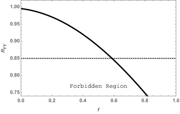
Figure 1: Predicted values of $R_{\gamma\gamma}$ (continuous line), as a function of the $f$ parameter, compared to the lower limit of the experimental value at 1$\sigma$ (dashed line). The region above the dashed line is allowed.

III.2 Searching for Resonances

We also consider the direct searches of resonances in the dijet and the dilepton channels. In the kinematic setup we have adopted (with very heavy non-standard scalars) only the spin-1 particle $V_{L}^{\pm},V_{L}^{0}$ (assumed to be degenerated) and $V_{R}^{0}$ can be produced in the $s$-channel by quark–anti-quark annihilation. At this point, we recall that the fields $V_{R}^{\pm}$ do not couple to the standard fermions. On the other hand, in the construction we are considering, $V_{R}$ cannot be heavier than $V_{L}$ (see equation (16)). Consequently, the model predicts that two resonances should appear in the dijet and the dilepton spectra with the lighter one corresponding to $V_{R}^{0}$.

III.2.1 Methodology

We implemented the model in CalcHEP Calchep using the LanHEP package Lanhep1 ; Lanhep2 and generate events for dijet and dilepton production at the 13 TeV LHC, considering only contribution of the new particles, without background, for several values of $M_{V_{L}}$and $M_{V_{R}}$. As an example, in Figure 2 we show two dijet spectra obtained in our simulations. In order to put constrains on the model parameter space, we count the events around each peak, we compute a cross section for each resonance and we compare it with the experimental upper limits for dijet or dilepton resonance cross-sections and we only accept a pair of $M_{V_{L}}$and $M_{V_{R}}$ values if the cross-section associated to each resonance is smaller than the experimental limit.

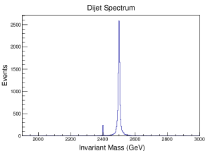
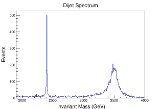
Figure 2: Examples of resonances in the dijet invariant mass spectrum. In this simulations has been taken into account only the contribution of the non-standard sector of the LBESS model without background.

III.2.2 Dijets

In the case of dijets, we use the limits provided by the ATLAS Collaboration based on data measures at $\sqrt{s}=13$ TeV AtlasDijet . Our results are shown in Figure 3. The region filled with black circles is the accepted zone, that is, the set of points $(M_{V_{L}},M_{V_{R}})$ which produce both resonances with a cross sections below the experimental limit. Notice that in the quasi-degenerate case, resonances with masses as light as 2000 or 2500 GeV are allowed. This is in agreement with previous studies on vector resonances AZ-1-2 ; AZ-2 ; AZ-3 .

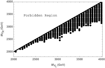
Figure 3: Constrains to the $(M_{V_{L}},M_{V_{R}})$ space by direct resonance searches in the dijets spectrum at the 13 TeV LHC. The region filled with black circles is the allowed one.

III.2.3 Dileptons

More stringent constrains are obtained in the dilepton channel. In this case, we use the limits provided by the ATLAS Collaboration at $\sqrt{s}=13$ TeV and 36.1 fb^-1AtlasDilepton . Again, the region filled by black circles is the accepted zone. In this case, only resonances heavier than 3.4 TeV are allowed. This improvement on the constrains is mainly due to the the fact that the dilepton production is a cleaner channel than dijet production at a hadron collider and the higher luminosity of the dilepton set of data.

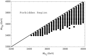
Figure 4: Constrains to the $(M_{V_{L}},M_{V_{R}})$ space by direct resonance searches in the dilepton spectrum at the 13 TeV LHC. The region filled with black circles is the allowed one.

III.3 Precision Tests

An indirect way to constrain extensions of the SM is to consider the contribution the new Physics provides to the electroweak radiative corrections. These effects are, in general, parametrized by the well known Peskin–Takeuchi parameters: $S$, $T$ and $U$. An equivalent set of parameters, named $\epsilon_{1}$, $\epsilon_{2}$ and $\epsilon_{3}$, is also used in the literature epsilon and is related to the former one by the following expressions:

$$\epsilon_{1} = \alpha T$$

$$\epsilon_{2} = -\frac{\alpha}{4s_{Z}^{2}}U$$ (2)

$$\epsilon_{3} = \frac{\alpha}{4s_{Z}^{2}}S$$

where $\alpha$ is the electromagnetic coupling constant at the scale of $M_{Z}$ and $s_{Z}^{2}$ is the $\sin^{2}\theta_{W}$ in the $\overline{MS}$ scheme at the same scale. In Ref. Casalbuoni:1997rs-1 , the following tree level expressions are provided for the $\epsilon_{i}$ parameters in the context of the LBESS model:

$$\epsilon_{1} = -rs_{\varphi}^{2}\frac{c_{\theta}^{4}+s_{\theta}^{4}}{c_{\theta}^{4}}$$

$$\epsilon_{2} = -rs_{\varphi}^{2}$$ (3)

$$\epsilon_{3} = -\frac{rs_{\varphi}^{2}}{c_{\theta}^{2}}$$

where $c_{\theta}=\cos\theta_{W}$, $s_{\theta}=\sin\theta_{W}$, while $r$ and $s_{\varphi}$ can be expressed in terms of $M_{V_{L}}$and $M_{V_{R}}$ as shown in the Appendix.

We use the values $S=0.05\pm 0.10$, $T=0.08\pm 0.12$ and $U=0.02\pm 0.10$ found in PDG , and the expressions above to select the combination of $M_{V_{L}}$and $M_{V_{R}}$ which reproduce simultaneously the experimental values of $\epsilon_{1}$, $\epsilon_{2}$ and $\epsilon_{3}$ (using equations (3)) within $1\sigma$. The result is shown in Fig. 5. The black region is the zone allowed by the precision variables. As we can see, the restrictions are not as stringent as the ones obtained using dilepton data.

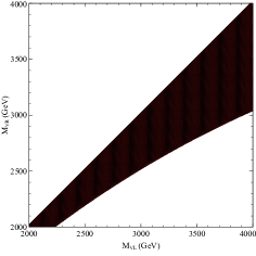
Figure 5: Constrains to the $(M_{V_{L}},M_{V_{R}})$ space by the electroweak precision tests. The black region is the allowed one.

IV Conclusions

We have studied the LBESS model in the context of recent data obtained at the 13 TeV LHC in the regime where the non-standard scalars are heavy with masses of the order of 3 TeV. We found that the value the $f$ parameter of the scalar potential has to belong to the interval $[0,0.6].$ Additionally, we have found that the model is consistent with current experimental data provided that the spin-1 resonances are heavier than 3.4 TeV. This limit is higher than the ones obtained in previous studies of models with vector resonances. The main restrictions come from recent searches of resonances in the dilepton spectrum.

Appendix

The LBESS model is based on the global symmetry $SU(2)_{L}\otimes SU(2)_{R}\otimes SU(2)_{L}^{\prime}\otimes SU(2)_{R}^{\prime}$ from which the subgroup $SU(2)_{L}\otimes U(1)\otimes SU(2)_{L}^{\prime}\otimes SU(2)_{R}^{\prime}$ is made local. The matter content consist of three scalars ($\Phi_{{\rm U}}$, $\Phi_{{\rm L}}$ and $\Phi_{{\rm R}}$) which we are supposed to be composite and the standard fermions (plus a right-handed neutrino). These fields transform under the global symmetry following the representation assignment showed in table 1 (scalars) and 2 (fermions). The representation assignment for fermions under the local symmetry is shown in table 3.

Fields	$SU(2)_{L}$	$SU(2)_{R}$	$SU(2)_{L}^{\prime}$	$SU(2)_{R}$
$\Phi_{{\rm U}}$	${\bf 2}$	${\bf\bar{2}}$	$1$	$1$
$\Phi_{{\rm L}}$	${\bf 2}$	$1$	${\bf 2}$	$1$
$\Phi_{{\rm R}}$	$1$	${\bf 2}$	$1$	${\bf 2}$

Table 1: Representations of the scalar fields under the full global group.

Fermion	$SU(2)_{L}$	$SU(2)_{R}$	$SU(2)_{L}^{\prime}$	$SU(2)_{R}^{\prime}$
$\Psi_{iL}$	${\bf 2}$	$1$	$1$	$1$
$\Psi_{iR}$	$1$	${\bf 2}$	$1$	$1$

Table 2: Representations of the fermion fields under the full global group.

Fermion	$SU(2)_{L}$	$U(1)$	$SU(2)_{L}^{\prime}$	$SU(2)_{R}^{\prime}$
$\Psi_{iL}$	${\bf 2}$	$Y^{\prime}$	$1$	$1$
$\Psi_{iR}$	$1$	$Y^{\prime}$	$1$	$1$

Table 3: Representations of the fermion fields under the full gauge group. Here $Y^{\prime}=B-L$ with $B$ and $L$ being the baryon and lepton numbers.

The full Lagrangian of model can be written down as:

$${\cal L} =\frac{1}{2}{\rm Tr}[F_{\mu\nu}(\tilde{W})F^{\mu\nu}(\tilde{W})]+\frac{1}{2}{\rm Tr}[F_{\mu\nu}(\tilde{B})F^{\mu\nu}(\tilde{B})]+\frac{1}{2}{\rm Tr}[F_{\mu\nu}(A_{L})F^{\mu\nu}(A_{L})]+\frac{1}{2}{\rm Tr}[F_{\mu\nu}(A_{R})F^{\mu\nu}(A_{R})]$$ (4)

$$+\frac{1}{4}\left[{\rm Tr}[(D_{\mu}\Phi_{{\rm U}})^{\dagger}(D^{\mu}\Phi_{{\rm U}})]+{\rm Tr}[(D_{\mu}\Phi_{{\rm L}})^{\dagger}(D^{\mu}\Phi_{{\rm L}})]+{\rm Tr}[(D_{\mu}\Phi_{{\rm R}})^{\dagger}(D^{\mu}\Phi_{{\rm R}})]\right]$$

$$-\mu^{2}({\rm Tr}[\Phi_{{\rm L}}^{\dagger}\Phi_{{\rm L}}]+{\rm Tr}[\Phi_{{\rm R}}^{\dagger}\Phi_{{\rm R}}])-\frac{\lambda}{4}([{\rm Tr}(\Phi_{{\rm L}}^{\dagger}\Phi_{{\rm L}})]^{2}+[{\rm Tr}(\Phi_{{\rm R}}^{\dagger}\Phi_{{\rm R}})]^{2})-m^{2}{\rm Tr}(\Phi_{{\rm U}}^{\dagger}\Phi_{{\rm U}})-\frac{h}{4}[{\rm Tr}(\Phi_{{\rm U}}^{\dagger}\Phi_{{\rm U}})]^{2}$$

$$-\frac{f_{3}}{2}{\rm Tr}(\Phi_{{\rm L}}^{\dagger}\Phi_{{\rm L}}){\rm Tr}(\Phi_{{\rm R}}^{\dagger}\Phi_{{\rm R}})-\frac{f}{2}[{\rm Tr}(\Phi_{{\rm L}}^{\dagger}\Phi_{{\rm L}}){\rm Tr}(\Phi_{{\rm U}}^{\dagger}\Phi_{{\rm U}})+{\rm Tr}(\Phi_{{\rm R}}^{\dagger}\Phi_{{\rm R}}){\rm Tr}(\Phi_{{\rm U}}^{\dagger}\Phi_{{\rm U}})]$$

$$+i\bar{\Psi}_{iL}\gamma^{\mu}D_{\mu}\Psi_{iL}+i\bar{\Psi}_{iR}\gamma^{\mu}D_{\mu}\Psi_{iR}+\bar{\Psi}_{iL}\Phi_{{\rm U}}\Upsilon\Psi_{jR}+{\rm h.c.}$$

where $\tilde{W}_{\mu},\tilde{B}_{\mu},A_{L\mu}$ and $A_{R\mu}$ are the gauge bosons associated to $SU(2)_{L}$, $U(1)$, $SU(2)_{L}^{\prime}$ and $SU(2)_{R}^{\prime}$, respectively and $\Upsilon$ is a matrix containing the Yukawa coupling constants. On the other hand, the strength tensors a defines as usual:

$$F_{\mu\nu}(\tilde{W}) =\partial_{\mu}\tilde{W}_{\nu}-\partial_{\nu}\tilde{W}_{\mu}+g_{0}[\tilde{W}_{\mu},\tilde{W}_{\nu}]$$ (5)

$$F_{\mu\nu}(\tilde{B}) =\partial_{\mu}\tilde{B}_{\nu}-\partial_{\nu}\tilde{B}_{\mu}$$

$$F_{\mu\nu}(A_{L}) =\partial_{\mu}A_{L\nu}-\partial_{\nu}A_{L\mu}+g_{2}[A_{L\mu},A_{L\nu}]$$

$$F_{\mu\nu}(A_{R}) =\partial_{\mu}A_{R\nu}-\partial_{\nu}A_{R\mu}+g_{2}[A_{R\mu},A_{R\nu}]$$

The covariant derivatives in the kinetic terms for the scalars and fermions in equation (4), are given by:

$$D_{\mu}\Phi_{{\rm L}} =\partial_{\mu}\Phi_{{\rm L}}+ig_{0}\frac{\tau^{a}}{2}\tilde{W}_{\mu}^{a}\Phi_{{\rm L}}-ig_{2}\Phi_{{\rm L}}\frac{\tau^{a}}{2}A_{L\mu}^{a}$$ (6)

$$D_{\mu}\Phi_{{\rm R}} =\partial_{\mu}\Phi_{{\rm R}}+ig_{1}\frac{\tau_{3}}{2}\tilde{B}_{\mu}\Phi_{{\rm R}}-ig_{2}\Phi_{{\rm R}}\frac{\tau^{a}}{2}A_{R\mu}^{a}$$

$$D_{\mu}\Phi_{{\rm U}} =\partial_{\mu}\Phi_{{\rm U}}+ig_{0}\frac{\tau^{a}}{2}\tilde{W}_{\mu}^{a}\Phi_{{\rm U}}-ig_{1}\Phi_{{\rm U}}\frac{\tau_{3}}{2}\tilde{B}_{\mu}$$

$$D_{\mu}\Psi_{iL} =(\partial_{\mu}+ig_{0}\tilde{W}_{\mu}^{a}\frac{\tau^{a}}{2}+\frac{i}{2}g_{1}Y^{\prime}\tilde{B}_{\mu})\Psi_{iL}$$ (7)

$$D_{\mu}\Psi_{iR} =(\partial_{\mu}+ig_{1}\tilde{B}_{\mu}\frac{\tau^{3}}{2}+\frac{i}{2}g_{1}Y^{\prime}\tilde{B}_{\mu})\Psi_{iR}$$

where $g_{0}$, $g_{1}$ and $g_{2}$ are the coupling constants associated to the groups $SU(2)_{L}$, $U(1)$ and $SU(2)_{L}^{\prime}\otimes SU(2)_{R}^{\prime}$ respectively.

For the aim of simplicity, it has been assumed an interchange symmetry between $\Phi_{{\rm L}}$ and $\Phi_{{\rm R}}$ in the potential and in the kinetic terms. Writing the scalars in “polar parametrization”, i.e. $\Phi_{{\rm L}}=\rho_{L}L$, $\Phi_{{\rm R}}=\rho_{R}R$ and $\Phi_{{\rm U}}=\rho_{U}U$ where $L$, $R$ and $U$ are unitary matrices, the potential gets a simpler form:

$$V(\rho_{U},\rho_{L},\rho_{R}) =2\mu^{2}\left[(\rho_{L}+u)^{2}+(\rho_{R}+u)^{2}\right]+\lambda\left[(\rho_{L}+u)^{4}+(\rho_{R}+u)^{4}\right]$$ (8)

$$+2m^{2}(\rho_{U}+v)^{2}+h(\rho_{U}+v)^{4}+2f_{3}(\rho_{L}+u)^{2}(\rho_{R}+u)^{2}$$

$$+2f(\rho_{U}+v)^{2}\left[(\rho_{L}+u)^{2}+(\rho_{R}+u)^{2}\right]$$

The scalar fields acquire a vacuum expectation value (vev): $\left\langle\rho_{U}\right\rangle=v$ and $\left\langle\rho_{L}\right\rangle=\left\langle\rho_{R}\right\rangle=u$ which spontaneously break the original gauge symmetry down to $U(1)_{{\rm em}}$.

In the true vacuum, nontrivial mass matrices appear in the scalar and the vector sector implying that the mass eigenstate are different from the “flavor” ones. In the case of scalar the relationship between flavor and mass eigenvectors is given, in in the limit $u\gg v$, by:

$$\begin{bmatrix}\rho_{L}\\ \rho_{R}\\ \rho_{U}\end{bmatrix} = \begin{bmatrix}\frac{1}{\sqrt{2}}&\frac{1}{\sqrt{2}}-\frac{q^{2}}{s_{\varphi}^{2}}r&-\frac{q}{s_{\varphi}}\sqrt{r}\\ -\frac{1}{\sqrt{2}}&\frac{1}{\sqrt{2}}(1-\frac{q^{2}}{s_{\varphi}^{2}}r)&-\frac{q}{s_{\varphi}}\sqrt{r}\\ 0&\frac{q}{s_{\varphi}}\sqrt{2r}&1-\frac{q^{2}}{s_{\varphi}^{2}}r\end{bmatrix}\begin{bmatrix}H_{L}\\ H_{R}\\ H\end{bmatrix}$$ (9)

where the variables $r$ and $q$ are

$$r=\frac{v^{2}}{u^{2}}\frac{g^{2}}{g_{2}^{2}}\leavevmode\nobreak\ \leavevmode\nobreak\ \leavevmode\nobreak\ \leavevmode\nobreak\ \leavevmode\nobreak\ \leavevmode\nobreak\ \leavevmode\nobreak\ \leavevmode\nobreak\ q=\frac{f}{f_{3}+\lambda}$$ (10)

,

$$s_{\varphi}=\sin(\varphi)=\frac{g_{0}}{\sqrt{g_{0}^{2}+g_{2}^{2}}}$$

and, $H_{L}$ and $H_{R}$ are the physical heavy scalar while $H$ denotes the standard-like Higgs boson.

The mass eigenvalues for the scalar fields, in the limit $u\gg v$, are given by:

$$M_{H}^{2} =8v^{2}(h-2\frac{f^{2}}{f_{3}+\lambda})$$ (11)

$$M_{H_{L}}^{2} =8u^{2}(\lambda-{f_{3}})$$

$$M_{H_{R}}^{2} =8u^{2}(\lambda+{f_{3}})$$

Similarly, in the vector sector, the relationship between flavor and mass eigenvectors is given by :

$$\begin{bmatrix}\tilde{W}^{\pm}\\ A_{L}^{\pm}\end{bmatrix}=\begin{bmatrix}c_{\varphi}(1-s_{\varphi}^{2}r)&-s_{\varphi}(1+c_{\varphi}^{2}r)\\ s_{\varphi}(1+c_{\varphi}^{2}r)&c_{\varphi}(1-s_{\varphi}^{2}r)\end{bmatrix}\begin{bmatrix}W^{\pm}\\ V_{L}^{\pm}\end{bmatrix}$$ (12)

$$\begin{bmatrix}\tilde{W}_{3}\\ \tilde{B}\\ A_{L}^{3}\\ A_{R}^{3}\end{bmatrix}=\begin{bmatrix}c_{\varphi}s_{\theta}&c_{\varphi}(c_{\theta}-\frac{s_{\varphi}^{2}}{c_{\theta}}r)&-s_{\varphi}(1+c_{\varphi}^{2}r)&\frac{c_{\varphi}s_{\varphi}s_{\theta}^{4}\sqrt{P}}{c_{\theta}^{3}(1-2c_{\theta}^{2})}r\\ \sqrt{P}&-\frac{s_{\theta}}{c_{\theta}}\sqrt{P}(1-\frac{s_{\varphi}^{2}s_{\theta}^{2}}{c_{\theta}^{4}}r)&-\frac{c_{\varphi}s_{\varphi}s_{\theta}\sqrt{P}}{1-2c_{\theta}^{2}}r&-\frac{s_{\varphi}s_{\theta}}{c_{\theta}}(1+\frac{s_{\theta}^{2}P}{c_{\theta}^{4}}r)\\ s_{\varphi}s_{\theta}&s_{\varphi}c_{\theta}(1+\frac{c_{\varphi}^{2}}{c_{\theta}^{2}}r)&c_{\varphi}(1-s_{\varphi}^{2}r)&-\frac{s_{\theta}^{2}P^{3/2}}{c_{\theta}^{3}(1-2c_{\theta}^{2})}r\\ s_{\varphi}s_{\theta}&-\frac{s_{\varphi}s_{\theta}^{2}}{c_{\theta}}(1+\frac{P}{c_{\theta}^{4}}r)&\frac{c_{\varphi}^{3}s_{\theta}^{2}}{1-2c_{\theta}^{2}}r&\frac{\sqrt{P}}{c}_{\theta}(1-\frac{s_{\varphi}^{2}s_{\theta}^{4}}{c_{\theta}^{4}}r)\end{bmatrix}\begin{bmatrix}A\\ Z\\ V_{L}^{0}\\ V_{R}^{0}\end{bmatrix}$$ (13)

Where, as usual $A$,$W^{\pm}$and $Z$ represent the photon and the standard weak gauge bosons while $V_{L}^{\pm,0}$ and $V_{R}^{\pm,0}$ are the physical heavy vector bosons and $\theta$ represents the Weinberg angle.

The mass eigenvalues of the vector sector are:

$$M_{A}^{2} =0$$ (14)

$$M_{Z}^{2} =\frac{v^{2}}{4}\frac{g^{2}}{c_{\theta}^{2}}(1-rs_{\varphi}^{2}\frac{1-2c_{\theta}^{2}+2c_{\theta}^{4}}{c_{\theta}^{4}}+\cdots)$$

$$M_{V_{L}^{0}}^{2} =\frac{v^{2}}{4}g^{2}(\frac{1}{rc_{\varphi}^{2}}+\frac{s_{\varphi}^{2}}{c_{\varphi}^{2}}-rs_{\varphi}^{2}\frac{c_{\theta}^{2}}{1-2c_{\theta}^{2}}+\cdots)$$

$$M_{V_{R}^{0}}^{2} =\frac{v^{2}}{4}\frac{g^{2}}{c_{\theta}^{2}}(\frac{1}{r}\frac{c_{\theta}^{4}}{P}+\frac{s_{\varphi}^{2}s_{\theta}^{4}}{P}+r\frac{s_{\varphi}^{2}s_{\theta}^{8}}{c_{\theta}^{4}(1-2c_{\theta}^{2})}+\cdots)$$

$$M_{V_{R}}^{2} =\frac{1}{4}g_{2}^{2}u^{2}$$

$$M_{W}^{2} =\frac{v^{2}}{4}g^{2}(1-rs_{\varphi}^{2}+\cdots)$$

$$M_{V_{L}}^{2} =\frac{v^{2}}{4}g^{2}(\frac{1}{r}\frac{1}{c_{\varphi}^{2}}+\frac{s_{\varphi}^{2}}{c_{\varphi}^{2}}+rs_{\varphi}^{2}+\cdots)$$

From the equations above it is easy to see that, when $u\gg v$, it is possible to write the $r$ parameter and $c_{\varphi}$in the convenient form:

$$r\thickapprox\frac{M_{W}^{2}}{M_{V_{R}}^{2}}$$ (15)

$$c_{\varphi}\approx\frac{M_{V_{R}}}{M_{V_{L}}}$$ (16)

Notice that due to the representation assignments, the fermions only couple to the gauge bosons $\tilde{W}$ and $B$ so their coupling to the heavy vector mass eigenstates arise only through mixing terms.

In this model, as shown in the Lagrangian, only Yukawa terms involve the fermions and the scalar field $\Phi_{{\rm U}}$ are allowed by the global symmetry. The Yukawa Lagrangian can be expanded as follows:

$${\cal L}_{Y}=\sum_{i.j}^{3}[y_{ij}^{d}(\bar{L}_{i}^{q}\Phi_{U})R_{j}^{d}+y_{ij}^{u}(\bar{L}_{i}^{q}\tilde{\Phi_{U}})R_{j}^{u}+y_{ij}^{l_{d}}(\bar{L}_{i}^{l}\Phi_{U})R_{j}^{l_{d}}+y_{ij}^{l_{u}}(\bar{L}_{i}^{l}\Phi_{U})R_{j}^{l_{u}}+{\rm h.c.}]$$ (17)

where the components of the scalar field are:

$$\Phi_{U}=\begin{bmatrix}iw^{+}\\ \frac{(v+\rho_{{\rm U}})+iz}{\sqrt{2}}.\end{bmatrix}$$ (18)

and

$$\rho_{U}=(1-\frac{q^{2}}{s_{\varphi}^{2}}r)H+\frac{q}{s_{\varphi}}\sqrt{2r}H_{R}.$$ (19)

It should also be noted that $\cos\varphi$ can be approximated to:

It is important to note that the parameters of the scalar potential have theoretical restrictions, which are described below:

$$\mu^{2} <0\leavevmode\nobreak\ \leavevmode\nobreak\ \leavevmode\nobreak\ \leavevmode\nobreak\ \leavevmode\nobreak\ \leavevmode\nobreak\ \leavevmode\nobreak\ \leavevmode\nobreak\ m^{2}<0\leavevmode\nobreak\ \leavevmode\nobreak\ \leavevmode\nobreak\ \leavevmode\nobreak\ \leavevmode\nobreak\ \leavevmode\nobreak\ \leavevmode\nobreak\ \leavevmode\nobreak\ f>0$$ (20)

$$\lambda-f_{3} >0\leavevmode\nobreak\ \leavevmode\nobreak\ \leavevmode\nobreak\ \leavevmode\nobreak\ \leavevmode\nobreak\ \leavevmode\nobreak\ h>f\frac{m^{2}}{\mu^{2}}\leavevmode\nobreak\ \leavevmode\nobreak\ \leavevmode\nobreak\ \leavevmode\nobreak\ \leavevmode\nobreak\ \leavevmode\nobreak\ \lambda+f_{3}>2f\frac{\mu^{2}}{m^{2}}$$

The restrictions for $\mu^{2}$ and $m^{2}$ are imposed so that the potential acquires a vacuum expectation value other than zero. On the other hand the restriction for $f$ comes from the decoupling of the model to the standard model with Higgs. The remaining restrictions in equation (20) derive from the positivity of the mass spectrum of the scalar fields.

Finally, we offer in table 4 a summary of the free parameters of the model.

Parameters	Meaning
$u$	Scale at which the extended symmetry breaks down
$f$	Parameter of quartic interactions in the potential
$M_{H_{L}}$	Mass of the heavy scalar $H_{L}$
$M_{H_{R}}$	Mass of the heavy scalar$H_{R}$
$M_{V_{L}}$	Mass of the heavy vector $V_{L}^{\pm},\leavevmode\nobreak\ \leavevmode\nobreak\ V_{L}^{0}$
$M_{V_{R}}$	Mass of the heavy vector $V_{R}^{\pm},\leavevmode\nobreak\ \leavevmode\nobreak\ V_{R}^{0}$

Table 4: Summary of the model’s free parameters

References

- (1) Casalbuoni R., De Curtis S., Dominici D. and Gatto R., Phys. Lett. B, 155 (1985) 95
- (2) Casalbuoni R., De Curtis S., Dominici D. and Gatto R., Nucl. Phys. B, 282 (1987) 235
- (3) R. Casalbuoni, S. De Curtis, D. Dominici and M. Grazzini, “An Extension of the electroweak model with decoupling at low-energy,” Phys. Lett. B 388, 112 (1996) doi:10.1016/0370-2693(96)01129-X [hep-ph/9607276].
- (4) R. Casalbuoni, S. De Curtis, D. Dominici and M. Grazzini, “New vector bosons in the electroweak sector: A Renormalizable model with decoupling,” Phys. Rev. D56, 5731 (1997) [hep-ph/9704229].
- (5) R. Foadi, M. T. Frandsen, T. A. Ryttov and F. Sannino, “Minimal Walking Technicolor: Set Up for Collider Physics,” Phys. Rev. D 76, 055005 (2007) doi:10.1103/PhysRevD.76.055005 [arXiv:0706.1696 [hep-ph]].
- (6) A. E. Carcamo Hernandez, C. O. Dib and A. R. Zerwekh, “The Effect of Composite Resonances on Higgs decay into two photons,” Eur. Phys. J. C , 2822 (2014) doi:10.1140/epjc/s10052-014-2822-6 [arXiv:1304.0286 [hep-ph]].
- (7) A. E. Cárcamo Hernández, B. Díaz Sáez, C. O. Dib and A. Zerwekh, “Constraints on vector resonances from a strong Higgs sector,” Phys. Rev. D 96 (2017) no.11, 115027 doi:10.1103/PhysRevD.96.115027 [arXiv:1707.05195 [hep-ph]].
- (8) M. Aaboud et al. [ATLAS Collaboration], “Measurements of Higgs boson properties in the diphoton decay channel with 36 fb-1 of collision data at TeV with the ATLAS detector,” arXiv:1802.04146 [hep-ex].
- (9) A. Belyaev, N. D. Christensen and A. Pukhov, “CalcHEP 3.4 for collider physics within and beyond the Standard Model,” Comput. Phys. Commun. 184, 1729 (2013) doi:10.1016/j.cpc.2013.01.014 [arXiv:1207.6082 [hep-ph]].
- (10) A. Semenov, “LanHEP: A Package for the automatic generation of Feynman rules in field theory. Version 3.0,” Comput. Phys. Commun. 180, 431 (2009) doi:10.1016/j.cpc.2008.10.012 [arXiv:0805.0555 [hep-ph]].
- (11) A. Semenov, “LanHEP — A package for automatic generation of Feynman rules from the Lagrangian. Version 3.2,” Comput. Phys. Commun. 201, 167 (2016) doi:10.1016/j.cpc.2016.01.003 [arXiv:1412.5016 [physics.comp-ph]].
- (12) The ATLAS collaboration [ATLAS Collaboration], “Search for New Phenomena in Dijet Events with the ATLAS Detector at TeV with 2015 and 2016 data,” ATLAS-CONF-2016-069.
- (13) O. Castillo-Felisola, C. Corral, M. González, G. Moreno, N. A. Neill, F. Rojas, J. Zamora and A. R. Zerwekh, “Higgs Boson Phenomenology in a Simple Model with Vector Resonances,” Eur. Phys. J. C 73, no. 12, 2669 (2013) doi:10.1140/epjc/s10052-013-2669-2 [arXiv:1308.1825 [hep-ph]].
- (14) The ATLAS collaboration [ATLAS Collaboration], “Search for new high-mass phenomena in the dilepton final state using 36.1 fb-1 of proton-proton collision data at TeV with the ATLAS detector,” JHEP 1710, 182 (2017) doi:10.1007/JHEP10(2017)182 [arXiv:1707.02424 [hep-ex]].
- (15) G. Altarelli and R. Barbieri, Phys. Lett. B253 , 161 (1991)
- (16) C. Patrignani et al. (Particle Data Group), Chin. Phys. C, 40, 100001 (2016) and 2017 update.