Constraints for the Progenitor Masses of Historic Core-Collapse Supernovae

Abstract

We age-date the stellar populations associated with 12 historic nearby core-collapse supernovae (CCSNe) and 2 supernova impostors, and from these ages, we infer their initial masses and associated uncertainties. To do this, we have obtained new HST imaging covering these CCSNe. Using these images, we measure resolved stellar photometry for the stars surrounding the locations of the SNe. We then fit the color-magnitude distributions of this photometry with stellar evolution models to determine the ages of any young existing populations present. From these age distributions, we infer the most likely progenitor mass for all of the SNe in our sample. We find ages between 4 and 50 Myr, corresponding to masses from 7.5 to 59 solar masses. There were no SNe that lacked a young population within 50 pc. Our sample contains 4 type Ib/c SNe; their masses have a wide range of values, suggesting that the progenitors of stripped-envelope SNe are binary systems. Both impostors have masses constrained to be $\;\buildrel<\over{\sim}\;$7.5 solar masses. In cases with precursor imaging measurements, we find that age-dating and precursor imaging give consistent progenitor masses. This consistency implies that, although the uncertainties for each technique are significantly different, the results of both are reliable to the measured uncertainties. We combine these new measurements with those from our previous work and find that the distribution of 25 core-collapse SNe progenitor masses is consistent with a standard Salpeter power-law mass function, no upper mass cutoff, and an assumed minimum mass for core-collapse of 7.5 M_⊙. The distribution is consistent with a minimum mass $<$9.5 M_⊙.

1. Introduction

Supernovae play a key role in nucleosynthesis, the formation of neutron stars and black holes, and in the morphological and chemical evolution of galaxies. The quantitative outcomes of these phenomena depends on which massive stars actually explode, and so it is important to constrain the distribution of massive stars that explode. However, their progenitors are difficult to study because supernovae are rare. Therefore, while there are well-developed theories of stellar evolution leading up to supernovae, these theories are difficult to test with observations that link SNe to their progenitor stars.

Stellar-evolution theory for isolated massive stars makes two basic predictions for core-collapse supernovae (CCSNe). First, the zero-age-main-sequence mass (M_ZAMS) and mass-loss history control whether a SN occurs, and second, the M_ZAMS determines the type of CCSN (Woosley et al., 2002a; Heger et al., 2003a; Dessart et al., 2011a). This theory predicts that the lower mass stars will explode with their hydrogen envelopes intact (e.g. II-P, II-L, IIn), and that the most massive stars lose much of their envelopes and explode as hydrogen deficient CCSNe (e.g. IIb, Ib/c).

Given the complexity of the underlying physics, however, especially binary evolution, winds, and episodic eruptions, it is unclear whether nature obeys the same well-delineated mass-dependence. In fact, recent theory (Claeys et al., 2011; Dessart et al., 2011a) and the relatively high observed rates of H-deficient CCSNe (Smith et al., 2011c) imply that binary evolution may figure prominently in producing the H-deficient CCSNe.

One sensitive test of theoretical SNe explosion mechanisms is the distribution of initial stellar masses that produce CCSNe. Unfortunately, the number of available progenitor masses of CCSNe with known spectral types is still relatively small, with each measurement having significance (e.g., Smartt, 2009; Maund et al., 2011a; Murphy et al., 2011; van Dyk et al., 2017; Davies & Beasor, 2017). At this point, about 32 CCSNe have progenitor mass constraints from direct precursor imaging, with many more having only upper bounds (e.g., Smartt, 2009; Gal-Yam & Leonard, 2009; Smith et al., 2011b; Maund et al., 2011a; Murphy et al., 2011; Fraser et al., 2012; Van Dyk et al., 2012a; Maund et al., 2014a; Fraser et al., 2014; Van Dyk et al., 2013, 2014; Smartt, 2015; Davies & Beasor, 2017; Van Dyk, 2017).

To increase the number of progenitor mass measurements available, we have been using a robust technique for constraining the progenitor ages for nearby historical CCSNe. We can measure these ages using resolved photometry of adjacent stellar populations from Hubble Space Telescope (HST) imaging taken at any time before or after the event (e.g., Badenes et al., 2009; Gogarten et al., 2009; Murphy et al., 2011; Williams et al., 2014b, hereafter W14; Maund, 2017). Our method relies on the fact that only relatively massive stars ($\;\buildrel>\over{\sim}\;$7.5 M_⊙) become CCSNe (Jennings et al., 2012). Thus, for single stars, their lifetimes are limited to $\;\buildrel<\over{\sim}\;$50 Myr (Girardi et al., 2002). Over 90% of stars form in clusters containing more than 100 members with $M_{\rm cluster}\!>\!50$ M_⊙ (Lada & Lada, 2003). These stars remain spatially correlated on physical scales up to $\sim$100 pc during the $100{\rm{\,Myr}}$ lifetimes of 4 M_⊙ stars, even if the cluster is not gravitationally bound (Bastian & Goodwin, 2006); we have confirmed this expectation empirically in several cases (Gogarten et al., 2009; Murphy et al., 2011, W14). Thus, it is reasonable to assume that any CCSN is physically associated with other young stars of the same age. This technique has significantly increased the sample of nearby SNe progenitor mass constraints for CCSNe with spectral types (Williams et al., 2014b; Maund, 2017).

Together, the progenitor masses measured to date suggest that the maximum mass for SN II-P may be lower than expected (Smartt et al., 2009). Counter to expectations, some H-rich CCSNe (in particular IIn) have been associated with more massive stars (Gal-Yam & Leonard, 2009; Smith et al., 2011b, c; Fox et al., 2017; Dwek et al., 2017). Furthermore, no progenitor mass of $>$20 M_⊙ has been established for any historical SNe with certainty, hinting at an upper mass cutoff [W14]. However, there are recent indications that no such maximum mass exists (e.g., Davies & Beasor, 2017), and may be the result of biases in analysis or sample size. Additional measurements are needed to significantly improve tests of any such cutoff.

We recently obtained new observations with HST of 12 more nearby CCSNe and 2 supernova impostors with known spectral types, allowing us to increase the number of color-magnitude diagram (CMD)-based constraints further. With this paper, the CMD-based sample is now up to 25 SNe (not including impostors), which we use to place constraints on the progenitor mass distribution.

In this paper, we describe our analysis of these new data and provide interpretations of the results in the context of massive stellar evolution and core-collapse supernova theory. Section 2 describes the data obtained and provides a brief summary of our analysis technique, which is already described in detail in previous papers. Section 3 details the results for our new constraints. Section 4 merges these results with previous measurements to investigate the shape of the progenitor mass distribution function, and section 5 concludes with a summary of our findings.

2. Data Acquisition and Analysis

Here we detail our sample selection, observations taken, resolved stellar photometry measurements, and stellar evolution model fitting.

2.1. Sample Selection

We selected all historical CCSNe within $8{\rm{\,Mpc}}$ with core-collapse spectral types that also have modest foreground extinction and arcsecond accuracy in their positions (Table 1). Such accuracy should be sufficient given the size of the apertures within which the CMD is constructed. We then cross-referenced the targets with the HST archive and identified those CCSNe that did not yet have adequate HST imaging, which are the 14 listed in Table 1.

The distances in the table are updated to include only tip of the red giant branch (TRGB) distances, which are the most appropriate to use for CMD fitting because it minimizes systematic offsets between the stellar evolution models and CMD features. Two of the SNe were in NGC 628, which had several distance measurements within 8 Mpc when we first developed the sample. However, the TRGB distance is 10 Mpc (Jang & Lee, 2014). This difference of 0.5 mag in depth results in us only reaching absolute magnitudes of -2 instead of -1.5 in these cases, which barely reaches the main-sequence turn-off for a 50 Myr population instead of reaching below it. We detected very few stars for those SNe, but we were still able to put constraints on the progenitors because those stars align well to a narrow range in young age. Thus, our technique appears to provide constrains even out to 10 Mpc.

Two other SNe (SN 2002bu and SN 2008S) might be SN impostors. We include these SN impostors because their classification is not definitive and because it is possible that these transients are also associated with the last stages of stellar evolution, in which case our proposed method to derive progenitor masses is still useful.

2.2. Observations

We provide a summary of our observations in Table 2, all from our program GO-14786. We observed 3 pointings in NGC 6946, covering 7 SNe, 1 pointing in NGC 628, covering 2 SNe, 1 pointing in NGC 4242 covering 1 SN, 1 pointing in NGC 1313 covering 1 SN, 1 pointing in NGC 4945 covering 1 SN, 1 pointing in NGC 4618 covering 1 SN, and 1 pointing in NGC 4214 covering 1 SN. We observed with ACS/WFC and WFC3/UVIS in parallel to provide the largest possible coverage of the host galaxies. For two of our pointings (NGC 628 and NGC 6946-3), this strategy allowed us to cover additional SNe locations in a single pointing. For others, it simply added coverage of these galaxies to the archive.

The exposure times and filters were selected to provide strong age constraints for the ages we are interested in ($<$50 Myr). These measurements require precise photometry of the main sequence stars produced at these ages. Our goal was to reach below the main-sequence turnoff for a 50 Myr population, which is M${}_{B}\,\sim$-2.5 and M${}_{V}\,\sim$-2.2, corresponding to m_B=28.3 and m_V=28.2 in NGC 6946, our most distant (m-M=28.9) and high extinction (E_B-V=0.34) target. We therefore have longer exposure times for our more distant target pointings. Our exposure dates, durations, and depths are provided in Table 2. We note that the observation we used for SN 2017eaw was a parallel exposure that was not intended for this program when we planned the observation. It is shallower than the other data, but serendipitously it turned out to be useful for constraining the progenitor mass of SN 2017eaw both from population analysis and precursor analysis.

2.3. Photometry

The photometry for this project was all performed using the DOLPHOT package (updated HSTphot Dolphin, 2000, 2016), through the same photometry pipeline used for the Panchromatic Hubble Andromeda Treasury, as described in Williams et al. (2014a). There have been a few updates to the photometry routine which we outline here. First, we now use the images that have been corrected for charge transfer efficiency effects (flc images) as inputs for our photometry instead of correcting our photometry catalogs for CTE effect after point spread function fitting. Second, we now use the TinyTim PSF libraries in DOLPHOT instead of the Anderson libraries, as rigorous testing found the TinyTim libraries to provide better spatial uniformity in DOLPHOT.

One key assumption of our technique is that the young populations within $\sim$50 pc of a SN location is coeval with the progenitor itself. Stellar cluster studies suggest that over 90% of stars form in clusters containing more than 100 members with $M\!>\!50$${\rm{\,M_{\odot}}}$(Lada & Lada, 2003). Furthermore, these stars likely remain spatially correlated on physical scales up to $\sim\!100{\rm{\,pc}}$ during the $100{\rm{\,Myr}}$. This spatial correlation continues even for low mass clusters that are not gravitationally bound (Bastian & Goodwin, 2006). Our previous studies (Gogarten et al., 2009; Murphy et al., 2011) have confirmed that this assumption is reasonable. We show some example CMDs of the data for the full field with the SNe location (within 50 pc) photometry overlaid in Figures 1 and 2. All of these are included as supplemental data for the article.

Using the same package, we also inserted and recovered artificial stars in the same regions as those extracted for population analysis around the locations of the SNe. These tests are performed by adding a star with known properties to the original images, and then rerunning the photometry on the images to determine if the star is recovered and how close the measured magnitude is to the true magnitude. By running many thousands of such tests within the region of the images containing the SNe locations, we can accurately model the photometric bias, error, and completeness as a function of color and magnitude. All of these quantities are required to fit the color-magnitude diagrams with those generated from models to derive the age distribution of the population, as described below.

2.4. Model Fitting

We fit all of our SNe locations using the software package MATCH 2.7 (Dolphin, 2002, 2012, 2013a). This package has been well-tested, and has been used in many studies for determining age distributions of stellar populations in external galaxies (e.g., Dolphin et al., 2003; Gallart et al., 2005; Williams et al., 2009; Weisz et al., 2011; Hillis et al., 2016; Skillman et al., 2017, and many others). We have also used it in many previous studies of progenitor mass estimates (Gogarten et al., 2009; Jennings et al., 2012, 2014; Williams et al., 2014b; Murphy et al., 2011).

In brief, the MATCH package generates model CMDs for a grid of ages and metallicities using the stellar evolution models of Girardi et al. (2002), updated by Marigo et al. (2008), and Girardi et al. (2010). We limited the recent star formation metallicities to be from one third solar to solar, as the upper main sequence feature is not very sensitive to metallicity, and the present day metallicities of these galaxies are not expected to be less than the Large Magellanic Cloud. In translating age to progenitor mass, this uncertainty in metallicity can make a difference of $<$10%.

The MATCH software convolves the model grid CMDs with the bias, uncertainty, and completeness measured with the artificial stars tests on the data. It applies extinction prescriptions supplied by the user, and finds the combination of the model CMD grid plus an optional background CMD that best fits the observed CMD of the region, where the weighting of the models corresponds to star formation rates for the various points in the age-metallicity grid.

The prescription for deriving extinction requires care. Each SNe likely resides in a region that is extincted by local dust, which causes differential extinction that spreads the photometry along the reddening vector of the CMD, as well as foreground dust that moves the entire CMD along the reddening line. To quantify these effects, we run a grid of model fits covering a range of overall extinction and differential extinction parameters. We then find the values for these parameters that provide the best fit to the data, and use those values for our final fit to the data. In most cases, the exact value of these parameters has little impact on the final age distribution. We show some examples of the impact of changing the extinction parameters in Figures 1 and 2.

The optional background CMD is important in galaxies with a large amount of global star formation, as is the case with several of our galaxies. In this case, we use the CMD of the entire field, which covers a much larger area of the galaxy. This background is then scaled by the ratio of the area of the SNe region to the area of the field (typically $<$0.001). In this way, if there is a widespread population with an age of, for example, 30 Myr, it will be down-weighted by the amount of stellar mass expected in the surrounding galaxy. If there is star formation at this age at a higher density than the background, it will still be the best-fit age; however, if there is star formation at this age, as well as at another age, the other age will be given a higher probability because of its absence from the global galaxy population. Use of this background CMD is a new addition to our technique, and it has helped to isolate the local population more clearly in some cases.

Once the best-fit is determined, the package has routines (hybridMC and zcombine) for performing Monte Carlo simulations and processing them to assess the uncertainties in the star formation rates for each age (Dolphin, 2013b). With this information about the star formation rates, we can determine the relative amount of stars present at each age. To measure this relative fraction, we study the cumulative distribution of the stellar mass with age. Because of the large amount of covariance between adjacent time bins in our technique (if the star formation increases in one time bin, it must decrease in the neighboring time bin for the total model to remain similar), the uncertainties on the star formation in each individual time bin tend to be large, making it difficult to interpret. However, these highly covariant uncertainties often result in a relatively clean cumulative distribution which is simpler to analyze.

We assume that only stars younger than 50 Myr are potential CCSN progenitors. This assumption means that we will only measure progenitor masses $>$7.3 M_⊙, which is reasonable given the minimum mass of 7.5 M_⊙ measured by Jennings et al. (2012). We first determine the total stellar mass present that is younger than this age. We then calculate the fraction of this total that is present at each age from 4 to 50 Myr, and assign this as the probability that the progenitor had that age. In most cases, there is a significant peak in the age distribution that allows us to constrain the age reliably. This age is only measured for the surrounding stars, and is therefore not dependent on the detailed evolution of the system itself. This age should therefore not be affected by, for example, the binarity of the progenitor or the uncertain physics of the last stages of stellar evolution.

Once we have the age measurement, we infer the mass of the progenitor using model stellar lifetimes (Girardi et al., 2002; Marigo et al., 2008; Girardi et al., 2010) as a function of stellar mass. For this step, we assume the progenitor was a single star. If the progenitor was in a mass-exchange binary, then the conversion from age to mass is less clear. Mass exchange can cause stars to evolve on different timescales than predicted from their initial masses because, for example, if a star that is initially 8 M_⊙ gains 5 M_⊙ in mass from a close companion, it may end its main sequence lifetime in significantly less time than an isolated 8 M_⊙ star. Thus, for such a system, our age to mass mapping will not provide a correct progenitor mass, but the progenitor age should still be useful for modeling the evolution of the progenitor. Whatever did explode, binary or single, it reached the end of its stellar lifetime at the age we have measured, so that if it is found to have been a binary, any model of the binary’s evolution would need to reproduce our measured lifetime.

3. Results

We show examples of the star formation histories used to determine the SN progenitor ages and masses in Figures 1 and 2. Similar plots for all of the SNe are supplied in the article supplemental data. Table 3 provides the best age and mass with uncertainties for each SN, and Table 4 gives the full age probability distribution for each SN for more rigorous statistical combinations.

The measurements for the older SNe may be somewhat less reliable due to the lower precision astrometry available for those events. However, as long as the astrometry is accurate to $\sim$1$"$, our extraction will contain the SN location, and the population will be representative. The fact that the measurements for these do not appear to be outliers in the mass distribution provides some assurance that our extraction regions for these events are appropriate. In one particular case (SN 1954A), we aligned the SN from the chart of Pietra (1955) to a 2MASS image of NGC 4214, and found that the position was consistent with that of Lennarz et al. (2012), which is the position we list is Table 1 to within an arcsec. We measured the age both at this location and the default location from the Open Supernova Catalog (which lists multiple reported locations). We found that while the median age changed substantially, it remained consistent within the large uncertainty for this SN. The new position has a high median mass, but a lower limit on the mass of $>$11 M_⊙.

It is important to note that the median age is not always the best representation of the mass probability, which is why we include the full probability distributions for each SN. Some of the SNe were in regions where more than one age was clearly present. Examples of these are SN 1948B and SN 1968D, which both had very young populations present of 10 Myr or younger, but these did not contain enough stellar mass to become the median age. In these cases, there is a possibility that the progenitor was younger ($8-10$ Myr) and more massive (20-30 M_⊙) which is only properly accounted for by using the full probability distribution we have included in Table 4.

For SNe with measurements here and in W14 (SN 1917A, SN 2004et, and SN 2005af) we prefer the measurement made here. The archival data are relatively poor in these cases (they had 7 stars or less in W14). For example, the previous measurement of SN 2005af was based on only 6 stars and found mass of 9${}^{+5}_{-1}$ M_⊙; however, with our new data we have 39 stars and a good background measurement, which argues for a 8 Myr old population above the background and pushes the best-fit mass to 38${}^{+1}_{-27}$ M_⊙. While the best fit changed significantly, the uncertainties of the measurements still overlap, as that slightly older population is still there at lower significance. SN 1917A went from 7 stars to 49 stars, and the mass went from 7.9${}^{+6.7}_{-0.5}$ to 15${}^{+1}_{-5}$. The measurement for SN 2004et went from 6 stars to 9 stars and the resulting mass estimate was equivalent to that in W14. Thus the measurements here are preferred to those of W14 for these SNe which had much shallower data prior to our new observations.

In one case (SN 2002bu) no young population was detected, suggesting a mass $<$7.3 M_⊙. Since this event was one of the likely impostors, this result is consistent with that possibility. The other possible impostor (SN 2008S) did have a young population present, but it has the lowest mass estimate of any of the SNe, which is also consistent with it being an impostor, since the mass estimate is below the standard limit for core-collapse progenitors. These results are consistent with previous work suggesting that SN 2002bu and SN 2008S are the same class of transient with relatively low mass progenitors (Szczygieł et al., 2012).

4. Discussion

Excluding the two impostors, we combine our new results with the other 13 non-impostor SNe from W14 and Murphy et al. (2011) to study the mass distribution. We compared these measurements to nine measurements from direct precursor imaging from the literature (Woosley & Phillips, 1988, SN 1987A,; Stancliffe & Eldridge, 2009, SN 1993J,; Hendry et al., 2005, SN 2003gd,; Wang et al., 2005, SN 2004dj,; Li et al., 2005, SN 2004et,; Maund et al., 2014b, SN 2005cs,; Maund et al., 2014, SN 2008bk,; Maund et al., 2011b, SN 2011dh,; Van Dyk, 2017, SN 2017eaw). We show a comparison to these measurements in Figure 3. There are other measurements that we could also compare, but we are not providing a complete review here. As examples, Van Dyk et al. (2002) constrained the mass of the SN 1993J progenitor; Crockett et al. (2011) provided another measurement of the progenitor mass of SN 2004et. Li et al. (2006) also provide an estimate of the SN 2005cs progenitor mass. Van Dyk et al. (2012b) provide a measurement of the SN 2008bk progenitor. There are also very recent measurements of progenitor masses in Davies & Beasor (2017).

Similar to W14, we find that the population-derived masses are consistent with the precursor imaging masses where both are available. The largest outlier is SN 2004et, which has a very young best-fit age by our technique. The upper limit on age is large enough that a significantly lower mass, similar to that found for the precursor, is allowed; however, if the best-fit age is correct, it would suggest the precursor colors were not well-modeled. For example, either poorly constrained pre-SN evolution, bolometric correction issues, or binary evolution could make the precursor colors difficult to interpret (Fuller, 2017; Davies & Beasor, 2017; Podsiadlowski, 1992). Overall, the sample size and uncertainties do not show any statistically-significant offset between the measurement techniques, and they rule out an offset of greater than $\sim$1 M_⊙.

Our lowest mass constraints are for the 2 supernova impostors in our sample. The two impostors in W14 (SN 1954J and SN 2002kg) were not the lowest of the sample, but neither were above 13 M_⊙. These therefore may be a different class of transient that results from more massive progenitors. The photometry and spectra of Humphreys et al. (2017) suggest that at least one of these (SN 2002kg) has a very massive (60$-$80 M_⊙) progenitor, which is somewhat at odds with surrounding populations.

The mass constraints from the surrounding populations should help us to shed light on their origins. We find that SN 1954J and SN 2002kg appear to have a different, more massive, progenitor type from SN 2002bu and SN 2008S, but not as massive as 50 M_⊙ (W14). There is a tendency to conflate some SN Impostors with luminous blue variables (LBVs, see Smith et al., 2011d, for a review). However, before our mass constraints there was some indication that SN 2002bu and SN 2008S may represent a lower mass class (Szczygieł et al., 2012; Adams et al., 2016). We note that even the stellar population ages associated with the more massive impostors, SN 1954J and SN 2002kg, are at odds with standard mass inferences for LBVs. If we assume single-star evolution, then the inferred masses for these impostors are $<$25 M_⊙. In contrast, the luminosity inferred mass for LBVs is 50 M_⊙ and greater (Smith et al., 2011d; Humphreys et al., 2017).

More recently, Smith & Tombleson (2015) noted that LBVs are isolated from other massive O stars and suggested that their evolution is dominated by binary evolution. Aghakhanloo et al. (2017) modeled this isolation and suggested that LBVs could be rejuvenated stars that started out as 20 M_⊙ and through binary evolution became more massive and more luminous. If this model is correct, the stellar populations surrounding LBVs should be significantly older than the luminosity-derived mass would predict. The impostors SN 1954J and SN 2002kg show exactly this discrepancy. From the luminosity, Humphreys et al. (2017) infer a mass of 60-80 M_⊙ for SN 2002kg. We find that the stellar ages are much older than the lifetime of such a massive star, leading to the lower inferred mass. LBVs and the most massive SN Impostors may be rejuvenated stars resulting from close binary evolution.

In Figure 4 we plot the mass distribution, color-coded by SN type, for all 25 CCSNe with population-derived progenitor mass estimates from this study and W14 (after removing the 2 likely impostors from this study and 2 more in W14). The complete distribution is consistent with standard stellar initial mass functions (IMFs). Along with the measured distribution are the resulting distributions from 100 draws of 25 masses from a Salpeter (1955) IMF and a lower mass limit of 7.5 M_⊙. The observed distribution overlaps significantly with many of the draws, so that a standard IMF is consistent with the data. A K-S test shows that half of these draws have a 50% or higher likelihood of being drawn from the same parent distribution as the measured masses. This consistency drops to just 10% of draws if we assume a minimum mass of 9.5 M_⊙. Thus, we can put a 90% confidence upper-limit on least massive stars to produce CCSNe of $<$9.5 M_⊙. Slightly steeper or shallower IMFs, such as those of Kroupa (2001) or Weisz et al. (2015), are similarly consistent with this sample of SNe. Thus, while we still do not have any mass constraint that conclusively rules out a progenitor of mass $\;\buildrel<\over{\sim}\;$20 M_⊙, these improved measurements and larger sample do not require an upper mass cutoff to the supernova progenitor mass distribution.

Finally, we see no clear association between SN type and progenitor mass. The type Ib/c SN appear randomly scattered in mass. There are two broad mechanisms for producing stripped massive stars that are progenitors to SN Ib/c (see Dessart et al., 2011b; Smith et al., 2011a, for a good discussion on these scenarios). In one, because mass loss has a stiff dependence on luminosity and mass, stars above about 30 solar masses lose their entire hydrogen envelopes and become Wolf Rayet stars, the progenitors to SN Ib/c (Langer et al., 1994; Woosley et al., 2002b; Heger et al., 2003b). In the second, binary interactions strip the hydrogen envelopes (Woosley et al., 1995; Yoon et al., 2010).

Recently, the observed mass-loss rates have been revised downward, making it more difficult to get the rates of WRs in single-star evolutionary models (Bouret et al., 2005). More recently, Smith et al. (2011a) noted that the rates of stripped envelope SNe are too high to attribute them to only stars with masses greater than 30 solar masses. They suggested that the binary evolution scenario is most consistent with the high rates of stripped-envelope SNe.

Since binary stripping is more sensitive to orbital parameters and less sensitive to the stars’ masses, the binary scenario would produce a relatively random and broad distribution of progenitor masses. The seemingly random and uniform distribution of ages and masses in our results is at odds with single-star evolutionary models and is most consistent with the binary evolution scenario. Taken together, all these recent results suggest that the progenitors of stripped envelope SNe are binary systems. However, we note that the full SFHs of these SNe do contain stars of the very youngest ages (see full probability distributions). Thus, while our results prefer type Ib/c progenitors of a variety of ages, with this sample of 4 we do not rule out high-mass progenitors for these SNe with confidence.

5. Conclusions

We have measured resolved stellar photometry around the locations of 12 historic CCSNe and 2 SN impostors. By fitting color-magnitude diagrams of this photometry, we have constrained the ages of the SN progenitor stars. Using these ages to infer progenitor masses, we have increased the sample of nearby CCSNe with progenitor mass constraints. With our full sample of 25 non-impostor measurements, we have compared the mass distribution to that of a standard mass function, such as a Salpeter (1955), Kroupa (2001), or Weisz et al. (2015). While the measured masses are somewhat below expectations from a standard mass function, they are consistent with such a parent distribution. Four of our sample are type Ib/c SNe, and we find that their progenitors are not the most massive. Instead, their ages and masses are uniformly distributed, which suggests that the progenitors of stripped-envelope SNe are binary systems.

Support for this work was provided by NASA through grant GO-14786 from the Space Telescope Science Institute, which is operated by the Association of Universities for Research in Astronomy, Incorporated, under NASA contract NAS5-26555.

Table 1SNe sample for this study. Positions taken from the Open Supernova Catalog (https://sne.space), except SN1954A and SN2003gd, which were taken from Pietra (1955) and Maund & Smartt (2009), respectively. Inclinations from the Bright Galaxy Catalog (de Vaucouleurs et al., 1991).

SN	RA	DEC	Galaxy	Incl. (deg.)	Type	Distance ($Mpc$)	Previous Measurement M⊙
SN 1917A	308.69542	60.12472	NGC 6946	32	II	6.8	7.9${}^{+6.7}_{-0.5}$ [W14]
SN 1948B	308.83958	60.17111	NGC 6946	32	IIP	6.8	None
SN 1954A	183.9445833	36.2630556	NGC 4214	39	Ib	3.0	None
SN 1968D	308.74333	60.15956	NGC 6946	32	II	6.8	None
SN 1978K	49.41083	-66.55128	NGC 1313	41	II	4.1	None
SN 1980K	308.875292	60.106597	NGC 6946	32	IIL	6.8	$\;\buildrel<\over{\sim}\;$18 (non-detection Thompson, 1982)
SN 1985F	190.38754	41.15164	NGC 4618	36	Ib	7.9	None
SN 2002ap	24.099375	15.753667	NGC 0628	24	Ic pec	10.0	$>$30 (non-detection Crockett et al., 2007)
							20$-$25 (SN properties Mazzali et al., 2002)
SN 2003gd	24.177708	15.738611	NGC 0628	24	IIP	10.0	8${}^{+4}_{-2}$ (precursor Hendry et al., 2005)
SN 2004et	308.85554	60.12158	NGC 6946	32	IIP	6.8	56${}^{+12}_{-40}$ [W14]
							17${}^{+2}_{-2}$ (Maund, 2017)
							15${}^{+5}_{-2}$ (precursor Li et al., 2005)
							8${}^{+5}_{-1}$ (precursor Crockett et al., 2011)
SN 2005af	196.18358	-49.56661	NGC 4945	79	IIP	3.6	8.5${}^{+0.5}_{-0.5}$ [W14]
SN 2017eaw	308.684333	60.193306	NGC 6946	32	IIP	6.8	$\sim$13 (precursor Van Dyk, 2017, preliminary)
SN 2002bu	184.40492	45.64650	NGC 4242	41	IIn	7.9	Possible Impostor (Kochanek et al., 2012)
SN 2008S	308.68896]	60.09939	NGC 6946	32	IIn?	6.8	Possible Impostor (Kochanek et al., 2012)

Table 2Pointing, Date, Filter, and Exposure Information for HST Observations

RA (J2000)	Dec (J2000)	Date	Galaxy	TARGNAME	Filter	Exp. Time (s)	Depth (mag)
308.866178	60.1141583	2015-10-08,2016-10-26	NGC 6946	NGC6946-3	F438W	5438	28.5
308.866178	60.1141583	2015-10-08,2016-10-26	NGC 6946	NGC6946-3	F606W	5777	28.2
308.723173	60.1844547	2016-10-26	NGC 6946	ANY	F606W	2430	28.5
308.723173	60.1844547	2016-10-26	NGC 6946	ANY	F814W	2570	27.2
308.801935	60.1712389	2016-10-28	NGC 6946	NGC6946-1	F435W	5610	28.1
308.801935	60.1712389	2016-10-28	NGC 6946	NGC6946-1	F606W	4478	27.5
308.740159	60.1185194	2016-11-03	NGC 6946	NGC6946-2	F435W	5610	28.6
308.740159	60.1185194	2016-11-03	NGC 6946	NGC6946-2	F606W	4488	27.9
24.1815463	15.7285792	2016-11-22	NGC 0628	SN2003GD	F438W	2510	29.1
24.1815463	15.7285792	2016-11-22	NGC 0628	SN2003GD	F606W	2400	27.8
24.0861567	15.7568500	2016-11-22	NGC 0628	SN2002AP	F435W	2300	28.3
24.0861567	15.7568500	2016-11-22	NGC 0628	SN2002AP	F606W	2194	28.1
184.404082	45.6430472	2016-11-26	NGC 4242	SN2002BU	F435W	2455	28.3
184.404082	45.6430472	2016-11-26	NGC 4242	SN2002BU	F606W	2320	27.9
190.386145	41.1467278	2016-11-27	NGC 4618	SN1985F	F435W	2410	26.6
190.386145	41.1467278	2016-11-27	NGC 4618	SN1985F	F606W	2280	26.2
183.945776	36.2811361	2017-01-25	NGC 4214	SN1954A	F435W	1360	28.1
183.945776	36.2811361	2017-01-25	NGC 4214	SN1954A	F606W	774	27.6

Table 3SNe Surrounding Population Median Age and Inferred Progenitor Mass Constraints

SN	Age (Myr)	$+$err	$-$err	Mass (M⊙)	$+$err	$-$err
SN 1917A	13	13	1	15	1	5
SN 1948B	28	2	13	10	4	1
SN 1954A	4.5	18	4.5	59	1	48
SN 1968D	28	4	14	9.6	4.2	0.6
SN 1978K	34	2	2	8.8	0.2	0.2
SN 1980K	32	1	20	9.0	6.7	0.2
SN 1985F	21	7	6	11.2	2.4	1.5
SN 2002ap	18	10	1	12.9	0.2	2.0
SN 2003gd	47	1	16	7.5	1.9	0.1
SN 2004et	4.7	18	1	47	2	36
SN 2005af	5.3	15	1	38	1	27
SN 2017eaw	33	2	9	8.8	2.0	0.2
SN 2002bu	$\cdots$	$\cdots$	$\cdots$	$\cdots$	$\cdots$	$\cdots$
SN 2008S	48	2	3	7.5	0.2	0.2

Table 4Age Statistics: Full Table Electronic Only.

Supernova	Low Age (Myr)	High Age (Myr)	Probability	$+$err	$-$err
SN1917A	4.0	4.5	0.000	0.017	0.000
SN1917A	4.5	5.0	0.071	0.000	0.071
SN1917A	5.0	5.6	0.000	0.088	0.000
SN1917A	5.6	6.3	0.000	0.091	0.000
SN1917A	6.3	7.1	0.000	0.095	0.000
SN1917A	7.1	7.9	0.000	0.099	0.000
SN1917A	7.9	8.9	0.000	0.109	0.000
SN1917A	8.9	10.0	0.000	0.140	0.000
SN1917A	10.0	11.2	0.000	0.186	0.000
SN1917A	11.2	12.6	0.000	0.309	0.000
SN1917A	12.6	14.1	0.865	0.000	0.865
SN1917A	14.1	15.8	0.000	0.613	0.000
SN1917A	15.8	17.8	0.000	0.588	0.000
SN1917A	17.8	20.0	0.000	0.565	0.000
SN1917A	20.0	22.4	0.000	0.549	0.000
SN1917A	22.4	25.1	0.000	0.506	0.000
SN1917A	25.1	28.2	0.000	0.454	0.000
SN1917A	28.2	31.6	0.064	0.335	0.064
SN1917A	31.6	35.5	0.000	0.308	0.000
SN1917A	35.5	39.8	0.000	0.246	0.000
SN1917A	39.8	44.7	0.000	0.184	0.000
SN1917A	44.7	50.1	0.000	0.118	0.000
SN1948B	4.0	4.5	0.000	0.014	0.000
SN1948B	4.5	5.0	0.000	0.025	0.000
SN1948B	5.0	5.6	0.017	0.032	0.017
$\cdots$	$\cdots$	$\cdots$	$\cdots$	$\cdots$	$\cdots$

Figure 1.— Example summary plots for our fitting technique for SN 1985F. These are available for all SN as supplemental material. Top Left: Cumulative fraction of stars at each age, as measured assuming different amounts of differential reddening. Each colored line shows the mass distribution measured assuming a different value of dAv. The color bar indicates the dAv values that correspond to the various colored lines. Top Middle: Quality of fit as a function of different amounts of assumed differential reddening. Lower values indicate a better fit to the data. Top Right: CMDs of the data. Grayscale shows the CMD of the background field (shade denotes log of number of data points in that CMD location). Outlined red points show the stars inside of the 50pc radius of the SN location. Blue dashed lines show the region of the CMD included in the fitting. Bottom Left: Cumulative fraction of total stellar mass younger than 50 Myr. The line shows the distribution corresponding to the best fit to the data. The shaded region shows all distributions consistent with the uncertainties as determined from the hybridMC routine. The quoted age and uncertainties correspond to the median age of the best fit (dashed line) along with all ages consistent with the median (red shading), considering the uncertainties. However, this single value with error does not always accurately capture the age distribution, so we include the full probability distribution in Table 4. Bottom Middle: The differential SFH, showing the rates and uncertainties in each age bin. This view is difficult to interpret directly because there are large covariances between adjacent age bins. Bottom Right: 25${}^{\prime\prime}{\times}25^{\prime\prime}$ HST image of the region surrounding the SN location. The orientation is North-up, East-left, and the 50 pc circle from which we took resolved stellar photometry for fitting is marked.

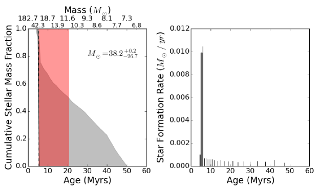
Figure 2.— Same as Figure 1 summary but for SN 2005af.

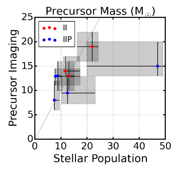
Figure 3.— Comparison of progenitor masses measured with direct precursor SED fitting vs those from our stellar population analysis where both measurements are available (taking measurements from here, Murphy et al., 2011, and W14). There is good agreement within the uncertainties in all cases. The farthest outlier is SN 2004et, which lies in a region with a young population with a large uncertainty in age, but best modeled by a very young age.

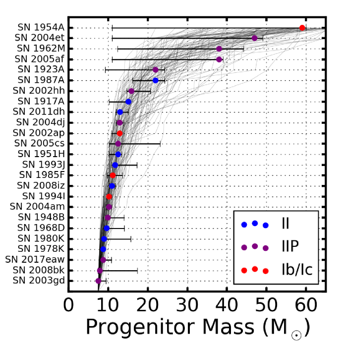
Figure 4.— The masses from the median ages, and their uncertainties, ranked by mass are shown with the points and error bars. Blue points show Type II SNe, and red points show Type Ib/c SNe. Likely impostors have not been included. The Type Ib/c SNe are not concentrated at the highest masses but randomly distributed in age and mass. This suggests that progenitors of stripped-envelope SNe are likely binary stars. Gray lines show draws of 25 stars from a Salpeter (1955) mass function without errors and a minimum mass of 7.5 M_⊙. The standard mass function, as well as a slightly steeper mass function such as that of Weisz et al. (2015), are fully consistent with the data.

References

- Adams et al. (2016) Adams, S. M., Kochanek, C. S., Prieto, J. L., Dai, X., Shappee, B. J., & Stanek, K. Z. 2016, MNRAS, 460, 1645
- Aghakhanloo et al. (2017) Aghakhanloo, M., Murphy, J. W., Smith, N., & Hložek, R. 2017, MNRAS, 472, 591
- Badenes et al. (2009) Badenes, C., Harris, J., Zaritsky, D., & Prieto, J. L. 2009, ApJ, 700, 727
- Bastian & Goodwin (2006) Bastian, N., & Goodwin, S. P. 2006, MNRAS, 369, L9
- Bouret et al. (2005) Bouret, J.-C., Lanz, T., & Hillier, D. J. 2005, A&A, 438, 301
- Claeys et al. (2011) Claeys, J. S. W., de Mink, S. E., Pols, O. R., Eldridge, J. J., & Baes, M. 2011, A&A, 528, A131
- Crockett et al. (2007) Crockett, R. M., et al. 2007, MNRAS, 381, 835
- Crockett et al. (2011) Crockett, R. M., Smartt, S. J., Pastorello, A., Eldridge, J. J., Stephens, A. W., Maund, J. R., & Mattila, S. 2011, MNRAS, 410, 2767
- Dalcanton et al. (2009) Dalcanton, J. J., et al. 2009, ApJS, 183, 67
- Davies & Beasor (2017) Davies, B., & Beasor, E. 2017, ArXiv e-prints,1709.06116
- de Vaucouleurs et al. (1991) de Vaucouleurs, G., de Vaucouleurs, A., Corwin, H. G., Jr., Buta, R. J., Paturel, G., & Fouqué, P. 1991, Third Reference Catalogue of Bright Galaxies. Volume I: Explanations and references. Volume II: Data for galaxies between 0h and 12h. Volume III: Data for galaxies between 12h and 24h. (Springer, New York, NY)
- Dessart et al. (2011a) Dessart, L., Hillier, D. J., Livne, E., Yoon, S.-C., Woosley, S., Waldman, R., & Langer, N. 2011a, MNRAS, 414, 2985
- Dessart et al. (2011b) Dessart, L., Hillier, D. J., Livne, E., Yoon, S.-C., Woosley, S., Waldman, R., & Langer, N. 2011b, MNRAS, 414, 2985
- Dolphin (2016) Dolphin, A. 2016, DOLPHOT: Stellar photometry, Astrophysics Source Code Library
- Dolphin (2000) Dolphin, A. E. 2000, PASP, 112, 1383
- Dolphin (2002) Dolphin, A. E. 2002, MNRAS, 332, 91
- Dolphin (2012) Dolphin, A. E. 2012, ApJ, 751, 60
- Dolphin (2013a) Dolphin, A. E. 2013a, ApJ, 775, 76
- Dolphin (2013b) Dolphin, A. E. 2013b, ApJ, 775, 76
- Dolphin et al. (2003) Dolphin, A. E., et al. 2003, AJ, 126, 187
- Dwek et al. (2017) Dwek, E., et al. 2017, ApJ, 847, 91
- Fox et al. (2017) Fox, O. D., et al. 2017, ApJ, 836, 222
- Fraser et al. (2012) Fraser, M., et al. 2012, ApJ, 759, L13
- Fraser et al. (2014) Fraser, M., et al. 2014, MNRAS, 439, L56
- Fuller (2017) Fuller, J. 2017, MNRAS, 470, 1642
- Gal-Yam & Leonard (2009) Gal-Yam, A., & Leonard, D. C. 2009, Nature, 458, 865
- Gallart et al. (2005) Gallart, C., Zoccali, M., & Aparicio, A. 2005, ARA&A, 43, 387
- Girardi et al. (2002) Girardi, L., Bertelli, G., Bressan, A., Chiosi, C., Groenewegen, M. A. T., Marigo, P., Salasnich, B., & Weiss, A. 2002, A&A, 391, 195
- Girardi et al. (2010) Girardi, L., et al. 2010, ApJ, 724, 1030
- Gogarten et al. (2009) Gogarten, S. M., Dalcanton, J. J., Murphy, J. W., Williams, B. F., Gilbert, K., & Dolphin, A. 2009, ApJ, 703, 300
- Grisé et al. (2008) Grisé, F., Pakull, M. W., Soria, R., Motch, C., Smith, I. A., Ryder, S. D., & Böttcher, M. 2008, A&A, 486, 151
- Heger et al. (2003a) Heger, A., Fryer, C. L., Woosley, S. E., Langer, N., & Hartmann, D. H. 2003a, ApJ, 591, 288
- Heger et al. (2003b) Heger, A., Fryer, C. L., Woosley, S. E., Langer, N., & Hartmann, D. H. 2003b, ApJ, 591, 288
- Hendry et al. (2005) Hendry, M. A., et al. 2005, MNRAS, 359, 906
- Hillis et al. (2016) Hillis, T. J., Williams, B. F., Dolphin, A. E., Dalcanton, J. J., & Skillman, E. D. 2016, ApJ, 831, 191
- Humphreys et al. (2017) Humphreys, R. M., Davidson, K., Van Dyk, S. D., & Gordon, M. S. 2017, ApJ, 848, 86
- Jang & Lee (2014) Jang, I. S., & Lee, M. G. 2014, ApJ, 792, 52
- Jennings et al. (2014) Jennings, Z. G., Williams, B. F., Murphy, J. W., Dalcanton, J. J., Gilbert, K. M., & Dolphin, A. E. 2014, ApJ, submitted
- Jennings et al. (2012) Jennings, Z. G., Williams, B. F., Murphy, J. W., Dalcanton, J. J., Gilbert, K. M., Dolphin, A. E., Fouesneau, M., & Weisz, D. R. 2012, ApJ, 761, 26
- Karachentsev et al. (2013) Karachentsev, I. D., Makarov, D. I., & Kaisina, E. I. 2013, AJ, 145, 101
- Karachentsev et al. (2000) Karachentsev, I. D., Sharina, M. E., & Huchtmeier, W. K. 2000, A&A, 362, 544
- Kochanek et al. (2012) Kochanek, C. S., Szczygieł, D. M., & Stanek, K. Z. 2012, ApJ, 758, 142
- Kroupa (2001) Kroupa, P. 2001, MNRAS, 322, 231
- Lada & Lada (2003) Lada, C. J., & Lada, E. A. 2003, ARA&A, 41, 57
- Langer et al. (1994) Langer, N., Hamann, W.-R., Lennon, M., Najarro, F., Pauldrach, A. W. A., & Puls, J. 1994, A&A, 290, 819
- Lennarz et al. (2012) Lennarz, D., Altmann, D., & Wiebusch, C. 2012, A&A, 538, A120
- Li et al. (2005) Li, W., Van Dyk, S. D., Filippenko, A. V., & Cuillandre, J.-C. 2005, PASP, 117, 121
- Li et al. (2006) Li, W., Van Dyk, S. D., Filippenko, A. V., Cuillandre, J.-C., Jha, S., Bloom, J. S., Riess, A. G., & Livio, M. 2006, ApJ, 641, 1060
- Marigo et al. (2008) Marigo, P., Girardi, L., Bressan, A., Groenewegen, M. A. T., Silva, L., & Granato, G. L. 2008, A&A, 482, 883
- Maund (2017) Maund, J. R. 2017, MNRAS, 469, 2202
- Maund et al. (2011a) Maund, J. R., et al. 2011a, ApJ, 739, L37
- Maund et al. (2011b) Maund, J. R., et al. 2011b, ApJ, 739, L37
- Maund et al. (2014) Maund, J. R., Mattila, S., Ramirez-Ruiz, E., & Eldridge, J. J. 2014, MNRAS
- Maund et al. (2014a) Maund, J. R., Reilly, E., & Mattila, S. 2014a, MNRAS, 438, 938
- Maund et al. (2014b) Maund, J. R., Reilly, E., & Mattila, S. 2014b, MNRAS, 438, 938
- Maund & Smartt (2009) Maund, J. R. & Smartt, S. J. 2009, Science, 324, 486
- Mazzali et al. (2002) Mazzali, P. A., et al. 2002, ApJ, 572, L61
- Monachesi et al. (2016) Monachesi, A., Bell, E. F., Radburn-Smith, D. J., Bailin, J., de Jong, R. S., Holwerda, B., Streich, D., & Silverstein, G. 2016, MNRAS, 457, 1419
- Murphy et al. (2011) Murphy, J. W., Jennings, Z. G., Williams, B., Dalcanton, J. J., & Dolphin, A. E. 2011, ApJ, 742, L4
- Pietra (1955) Pietra, S. 1955, Mem. Soc. Astron. Italiana, 26, 185
- Podsiadlowski (1992) Podsiadlowski, P. 1992, PASP, 104, 717
- Salpeter (1955) Salpeter, E. E. 1955, ApJ, 121, 161
- Skillman et al. (2017) Skillman, E. D., et al. 2017, ApJ, 837, 102
- Smartt (2009) Smartt, S. J. 2009, ARA&A, 47, 63
- Smartt (2015) Smartt, S. J. 2015, PASA, 32, e016
- Smartt et al. (2009) Smartt, S. J., Eldridge, J. J., Crockett, R. M., & Maund, J. R. 2009, MNRAS, 395, 1409
- Smith et al. (2011a) Smith, N., Li, W., Filippenko, A. V., & Chornock, R. 2011a, MNRAS, 412, 1522
- Smith et al. (2011b) Smith, N., et al. 2011b, ApJ, 732, 63
- Smith et al. (2011c) Smith, N., Li, W., Silverman, J. M., Ganeshalingam, M., & Filippenko, A. V. 2011c, MNRAS, 415, 773
- Smith et al. (2011d) Smith, N., Li, W., Silverman, J. M., Ganeshalingam, M., & Filippenko, A. V. 2011d, MNRAS, 415, 773
- Smith & Tombleson (2015) Smith, N., & Tombleson, R. 2015, MNRAS, 447, 598
- Stancliffe & Eldridge (2009) Stancliffe, R. J., & Eldridge, J. J. 2009, MNRAS, 396, 1699
- Szczygieł et al. (2012) Szczygieł, D. M., Kochanek, C. S., & Dai, X. 2012, ApJ, 760, 20
- Thompson (1982) Thompson, L. A. 1982, ApJ, 257, L63
- Tikhonov (2014) Tikhonov, N. A. 2014, Astronomy Letters, 40, 537
- Van Dyk (2017) Van Dyk, S. D. 2017, Philosophical Transactions of the Royal Society of London Series A, 375, 20160277
- Van Dyk et al. (2012a) Van Dyk, S. D., et al. 2012a, AJ, 143, 19
- Van Dyk et al. (2012b) Van Dyk, S. D., et al. 2012b, AJ, 143, 19
- van Dyk et al. (2017) van Dyk, S. D., Filippenko, A. V., Fox, O. D., Kelly, P. L., Milisavljevic, D., & Smith, N. 2017, The Astronomer’s Telegram, No. 10378, 378
- Van Dyk et al. (2002) Van Dyk, S. D., Garnavich, P. M., Filippenko, A. V., Höflich, P., Kirshner, R. P., Kurucz, R. L., & Challis, P. 2002, PASP, 114, 1322
- Van Dyk et al. (2013) Van Dyk, S. D., et al. 2013, ApJ, 772, L32
- Van Dyk et al. (2014) Van Dyk, S. D., et al. 2014, AJ, 147, 37
- Wang et al. (2005) Wang, X., Yang, Y., Zhang, T., Ma, J., Zhou, X., Li, W., Lou, Y.-Q., & Li, Z. 2005, ApJ, 626, L89
- Weisz et al. (2011) Weisz, D. R., et al. 2011, ApJ, 739, 5
- Weisz et al. (2015) Weisz, D. R., et al. 2015, ApJ, 806, 198
- Williams et al. (2009) Williams, B. F., et al. 2009, AJ, 137, 419
- Williams et al. (2014a) Williams, B. F., et al. 2014a, ApJS, 215, 9
- Williams et al. (2014b) Williams, B. F., Peterson, S., Murphy, J., Gilbert, K., Dalcanton, J. J., Dolphin, A. E., & Jennings, Z. G. 2014b, ApJ, 791, 105
- Woosley et al. (2002a) Woosley, S. E., Heger, A., & Weaver, T. A. 2002a, Reviews of Modern Physics, 74, 1015
- Woosley et al. (2002b) Woosley, S. E., Heger, A., & Weaver, T. A. 2002b, Reviews of Modern Physics, 74, 1015
- Woosley et al. (1995) Woosley, S. E., Langer, N., & Weaver, T. A. 1995, ApJ, 448, 315
- Woosley & Phillips (1988) Woosley, S. E., & Phillips, M. M. 1988, Science, 240, 750
- Yoon et al. (2010) Yoon, S.-C., Woosley, S. E., & Langer, N. 2010, ApJ, 725, 940