footnote \headersOptimized mixing by cutting-and-shufflingL. D. Smith, P. B. Umbanhowar, J. M. Ottino, and R. M. Lueptow
Optimized mixing by cutting-and-shuffling††thanks: Submitted to the editors . \fundingP.B. Umbanhowar was partially supported by the National Science Foundation Contract No. CMMI-1435065.
Abstract
Mixing by cutting-and-shuffling can be understood and predicted using dynamical systems based tools and techniques. In existing studies, mixing is generated by maps that repeat the same cut-and-shuffle process at every iteration, in a “fixed” manner. However, mixing can be greatly improved by varying the cut-and-shuffle parameters at each step, using a “variable” approach. To demonstrate this approach, we show how to optimize mixing by cutting-and-shuffling on the one-dimensional line interval, known as an interval exchange transformation (IET). Mixing can be significantly improved by optimizing variable protocols, especially for initial conditions more complex than just a simple two-color line interval. While we show that optimal variable IETs can be found analytically for arbitrary numbers of iterations, for more complex cutting-and-shuffling systems, computationally expensive numerical optimization methods would be required. Furthermore, the number of control parameters grows linearly with the number of iterations in variable systems. Therefore, optimizing over large numbers of iterations is generally computationally prohibitive. We demonstrate an ad hoc approach to cutting-and-shuffling that is computationally inexpensive and guarantees the mixing metric is within a constant factor of the optimum. This ad hoc approach yields significantly better mixing than fixed IETs which are known to produce weak-mixing, because cut pieces never reconnect. The heuristic principles of this method can be applied to more general cutting-and-shuffling systems.
keywords:
mixing optimization, cutting-and-shuffling, interval exchange transformation37A25, 49J21, 49K21, 49N90
1 Introduction
Cutting-and-shuffling has recently been shown to be an effective method for mixing granular materials [40, 39, 16, 15, 5, 28, 27, 34, 38, 46] and fluids [35, 37, 14, 30, 31, 13, 3]. However, previous studies only consider systems where the same cut-and-shuffle action is repeated at every step, for example, cutting a deck of cards at the 10th and 20th cards, and swapping the top pile with the bottom pile. Repeating this cut-and-shuffle could potentially transform an unmixed deck of cards (e.g., organized by suit) into a “mixed” state (no two cards of the same suit together). However, it seems likely that a mixed state would be reached faster if the locations of the cuts were chosen strategically at each step. Here we explore how this can be accomplished.
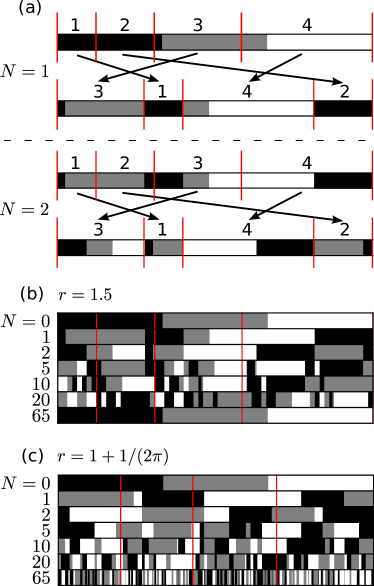
Consider the simplest form of cutting-and-shuffling for a continuous system: cutting a 1D line interval into pieces, and permuting them to reassemble the line. An example of this process, known as an Interval Exchange Transformation (IET), is shown in Fig. 1(a), where the line, initially consisting of equal length black, gray and white segments, is cut into four pieces, and the permutation represents the rearrangement order of the four cut pieces. The notation means that the third cut piece moves to the first position, the first piece moves to the second position, fourth piece moves to third position, and second piece moves to fourth position. In the second iteration, , the same cut locations and permutations are used. We refer to IETs with the same cut locations and permutation at every iteration as “fixed,” since the same action is repeated; these can be thought of as analogues of time-periodic fluid flows. Fixed IETs like that in Fig. 1(a) can generate good mixing.
While fixed IETs can produce mixing, i.e. complete homogenization of material given infinite time [18, 19, 43], mixing by cutting-and-shuffling occurs at best at a polynomial rate, which is significantly slower than the exponential mixing rates produced by chaotic systems [42, 17, 23, 2, 39, 4]. To demonstrate, consider the time-space plots shown in Fig. 1(b,c). Here, the iterates of the 1D line interval under the cut-and-shuffle operation are stacked so that the initial condition () is at the top and iteration is at the bottom (many intermediate iterates have been omitted). When the lengths of the cut pieces are rationally dependent [Fig. 1(b)], or the permutation is reducible***A permutation is said to be irreducible if applying to any of the subsets does not yield a permutation of just the elements of that subset. A permutation that is not irreducible is termed reducible., the colors do not mix well. In fact, the colors reassemble to their initial condition for the example in Fig. 1(b). When the lengths of the cut pieces are rationally independent, and the permutation is irreducible and not a rotation, the IET satisfies the Keane minimality condition [18, 19, 43] and yields good mixing of the colors [Fig. 1(c)]. However, additional parametric freedom in the mixing process can be introduced by allowing the cut locations and/or permutation to change at every iteration. We call this approach “variable,” and it is analogous to time-dependent fluid flow, which changes at every instant. In this study we consider variable IETs such that the permutation is fixed, but the cut locations can vary. Intuitively, the additional control freedom at each iteration should enable faster and better mixing when using variable IETs rather than fixed IETs.
Finding the best variable protocol is an optimal control problem. That is, the goal is to minimize or maximize an objective function (the degree, rate, or efficiency of mixing) over the parameter space. Optimal mixing has been studied for time-dependent laminar fluid flows [6, 10, 11, 24, 29, 44, 26], in which mixing occurs by stretching-and-folding. Here we consider optimal mixing by cutting-and-shuffling. There are a number of differences between mixing produced by cutting-and-shuffling compared to traditional mixing produced by stretching-and-folding. To start with, cutting-and-shuffling results in discontinuous interfaces when applied to a scalar field, even when the initial scalar field is smooth. This means mixing can be highly sensitive to parameter choices, even for a single iteration. In addition, standard mixing metrics such as the mix-norm [25], intensity of segregation [7], and interface length [22] do not vary smoothly, or even continuously, across the parameter space, which poses unique challenges in applying optimal control theory to cutting-and-shuffling.
In Section 2.1, we discuss different metrics that can be used to quantify mixing by IETs. A new metric is introduced that quantifies how well the colored segments are broken up into smaller segments and whether the different colors are evenly distributed along the line. We demonstrate that neither weak-mixing fixed IETs, nor a naive, ad hoc, variable approach – cutting the longest segments of each color in half at each iteration – yield optimal mixing.
In Section 2.2, we demonstrate how to analytically find optimal variable IETs with fixed permutation but variable cut locations. We show that optimal mixing can only be produced when the permutation takes a specific form, and demonstrate how to find cut locations that achieve optimal mixing. Then in Section 3 we show that optimal variable IETs produce significantly better mixing than general fixed IETs, and when the initial condition is more complex, there is more improvement gained by using an optimal variable IET compared to both random fixed IETs and optimal fixed IETs.
In Section 4, we discuss strategies for mixing by cutting-and-shuffling over many iterations. For general cutting-and-shuffling systems, both fixed and variable, finding protocols that optimize mixing over many iterations can be computationally expensive. One alternative option to achieve good, though sub-optimal, mixing is to use geometric properties of fixed piecewise isometries. For instance, fixed IETs that satisfy the Keane minimality condition [18, 43, 2], such as in Fig. 1(c), yield weak-mixing. However, for initial conditions like the three-color initial condition in Fig. 1, it is likely that a weak-mixing fixed IET will produce slow mixing, since identically colored segments sometimes reconnect after the cut pieces are shuffled. This means colored segments will not always be broken into smaller and smaller pieces. Another alternative is to optimize over short time-horizons. We demonstrate this approach for IETs using the computationally inexpensive ad hoc method introduced in Section 2.1, which is equivalent to a one-iteration time-horizon optimization. This ad hoc method produces significantly better mixing than weak-mixing fixed IETs, because segments of the same color never reconnect. Similar heuristic approaches could be applied to more general cutting-and-shuffling systems, cutting the largest unmixed regions at each iteration.
2 Optimal variable cutting-and-shuffling
2.1 Mixing metrics
Optimization of mixing requires a mixing metric. Qualitatively, for IETs with more than two differently colored segments, mixing is effective if the segments are broken up into many smaller segments and the different colors are evenly distributed along the line. Thinking of a deck of cards, the suits would be considered well mixed if any set of four consecutive cards contains one card of each suit.
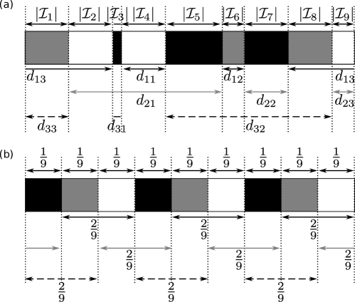
For a line interval consisting of colored segments, , with lengths as shown in Fig. 2(a), one mixing metric used previously is the longest segment length
| (1) |
termed the percent unmixed [21, 45]. For example, in Fig. 2(a), and in Fig. 2(b). Note that we assume periodic boundary conditions at the ends of the line, so segments of the same color at the start and end of the line are connected. Using periodic boundaries means that is invariant under rotations (left or right shifts). The same periodic boundary conditions have also been used in past studies [1, 39, 10]. Finding IETs that minimize ensures that all the segment lengths are small, suggesting good mixing, but does not consider whether the colors are distributed evenly along the line. For the deck of cards analogy, is minimized if every set of two consecutive cards have different suits, but this can be achieved by riffling the hearts and diamonds, and riffling the spades and clubs. Even though is minimized, the deck would not be considered mixed, as all the red cards are separate from all the black cards.
To measure the evenness of color distribution, we calculate the longest distance between segments of the same color. Letting represent the distance between the closest edges of the -th and -th segments of the -th color, where spans the number of different colors and spans the number of segments with the -th color, the evenness metric is
| (2) |
In Fig. 2(a), , and in Fig. 2(b), . When the colors are evenly distributed is small, and when they are clustered together is large. Note that if there are only two colors, then and are identical, otherwise they are generally different.
For an IET that starts with differently colored segments and uses a length permutation, at most new segments are created per iteration. Therefore, there are at most total segments after iterations, and has a minimum of , when all the segments are equal length. We scale by its minimum value,
| (3) |
to measure how well an IET has cut the colored segments into smaller pieces compared to the known optimum. Values of greater than correspond to suboptimal cutting of the colored segments into smaller pieces. Similarly, is minimized when there are differently colored segments between each pair of same-colored segments [e.g., Fig. 2(b)], and each segment has length , so we scale :
| (4) |
Values of greater than correspond to uneven distributions of the different colors.
For mixing colors on the line, there are two competing interests – small segment lengths () and evenly distributed colors () – and an optimal protocol for one metric is not necessarily an optimal for the other. We use simple linear scalarization to handle this multi-objective optimization task by defining the metric, as the total measure of mixing. Values of greater than mean that either the segments are not cut into small pieces or the colors are not evenly distributed, or both. When segments are equal in length and colors are uniformly distributed, .
Considering the fixed IET in Fig. 1(c), even though it is known to be weak-mixing (i.e. given an infinite number of iterations it will completely homogenize the colors), we see that after 65 iterations mixing is suboptimal. Only segments are produced, compared to the maximum . In addition, the segments are clearly not equal in length, quantified by , meaning the longest segment is more than three times longer than in an optimal case. Similarly, the colors are not well distributed, . There appears to be a darker region near the middle of the line, where black segments are clustered together, and a lighter region near the right-hand end, where white segments are clustered together. In this case, is significantly higher than an optimal variable IET for which .
For a given number of cuts and a given number of initial colors, optimal mixing corresponds to evenly distributed segments of equal length like the case shown in Fig. 2(b). The question is: Can variable IETs be found that achieve optimal mixing? A naive, ad hoc, approach, is to cut the longest segments in half at each iteration. This is demonstrated for the two-color initial condition in Fig. 3, where the longest black and gray segments at each iteration are cut in half, and the pieces are rearranged according to the permutation . For such a simple approach, this method performs remarkably well. Whenever , the segments all have equal length, and the maximum number of segments, , has been created, meaning ( in Fig. 3). However, for any other value of , mixing is suboptimal. For instance, at (the bottom row of Fig. 3). In the next section, we demonstrate how to find optimal variable IETs ().
2.2 Finding optimal variable IETs
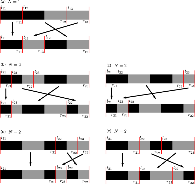
Consider the two-color initial condition with the first half of the line colored black, and the second half gray [top row of Fig. 4(a)], and a variable IET that cuts the line into pieces, with the -th cut in the -th iteration located at , and rearranges the cut pieces according to a permutation . After cutting, but before rearrangement, there are cut pieces, each with a left edge and a right edge. After rearrangement, new segments and new interfaces can only be created if left and right edges of different colors join. Hence, at most new segments/interfaces can be created (taking into account the existing interface in the initial condition between the start and end of the line). For example, the permutation has three cut pieces, and creates at most two new segments per iteration, as demonstrated in Fig. 4(a). Therefore, after iterations there can be at most new segments. However, not all variable IETs produce new segments per iteration, the trivial example being any IET that uses the identity permutation, which cuts but does not shuffle, leaving the line unchanged regardless of the cut locations. Similarly, rotation permutations, i.e. those of the form , do not shuffle, and so cannot produce new segments [45]. The following proposition gives the necessary and sufficient conditions for a variable IET to be able to produce new segments per iteration.
Proposition 2.1.
For the left-right two-color initial condition, there exists a variable IET that creates new segments per iteration if and only if is odd and is of the form
| (5) |
where , is a permutation of the set , is a permutation of the set , and , or is a rotation of a permutation of this form.
By a rotation of a permutation , we mean a permutation of the form for some . For example, the rotations of the permutation are , , and . The rotated permutation is the composition , where is the rotation permutation .
As an example of Proposition 2.1, for , choose , , and , then
| (6) |
By Proposition 2.1, there exist cut locations such that the corresponding variable IET, , creates new segments per iteration. The same is true for any rotation of , e.g. .
Corollary 2.2.
For odd, there are permutations for which there is a variable IET that can produce new segments per iteration.
Proof 2.3.
There are choices for the permutation , choices for the permutation , choices for , and rotations of a permutation of length . Therefore, the number of rotations of permutations of the form Eq. 5 is
| (7) |
We prove Proposition 2.1 using the following results.
Proposition 2.4.
For the left-right two-color initial condition and a permutation with length , if there exist cut locations , , such that cutting and rearranging the initial condition according to yields new segments, then there exist cut locations for all and such that the corresponding variable IET, , creates new segments per iteration.
Proof 2.5.
Suppose there exist cut locations , , such that cutting and rearranging the initial condition according to produces new segments. Let denote the colors of the left edges of the cut pieces for the -th iteration, and denote the colors of the right edges of the cut pieces. From the initial condition, we know is black (the left edge of the line) and is gray (the right edge of the line), and since new segments are created after rearrangement by , each left edge must join with a differently colored right edge, i.e. for . After rearrangement there are two cases, either the left-most segment is black or gray. If the left-most segment is black, for the second iteration choose the cut locations , , such that the left and right edges satisfy and , respectively, for . It follows that after rearrangement by , adjacent segments satisfy , so each left edge joins with a differently colored right edge, and new segments have been created.
If the left-most segment is gray, for the second iteration choose the cut locations , , such that the left and right edges satisfy and , i.e. the left and right edges of cut pieces have the opposite colors to the first iteration. Again, must join every left edge with a differently colored right edge, since that was the action in the first iteration. Choosing the opposite color sequence is equivalent to switching the two colors (black segments become gray, and vice versa), then performing the cut and shuffle, and then switching the two colors back.
In successive iterations, as long as the cut locations are chosen such that the left edges and right edges of cut pieces have the colors and (or their opposites if the first colored segment at the -th iteration is gray), then new segments will be created.
For example, for the two-color initial condition, variable IETs with permutation create two new segments in the first iteration, , as long as the first cut is in the black segment and the second cut is in the gray segment, as shown in Fig. 4(a). In successive iterations, , two new segments are created if the first cut is in a black segment, and the second cut is in a gray segment, as shown in Fig. 4(b–d) for . Note that the cuts do not need to occur in the first black and gray segments, e.g., Fig. 4(c,d).
Proposition 2.4 shows that the creation of new segments only depends on the colors of the edges of the cut pieces, and does not depend on the colors within the interior of each cut piece.
From Proposition 2.4, it suffices to consider only whether there exist cut locations for a permutation that can create new segments in the first iteration.
Proposition 2.6.
For a permutation , if there exist cut locations such that the corresponding variable IET yields new segments per iteration, then for any rotation of , there exist cut locations such that yields new segments per iteration.
Proof 2.7.
The action of the IET with permutation , i.e. is a rotation of , is to perform the rearrangement of the cut pieces by , and then shift all the segments along the line. Therefore, if new segments are created in the first iteration by with cuts , then the same number of segments is created by with cuts . From Proposition 2.4 there exist cut locations for all such that produces new segments per iteration.
Therefore, we need only consider permutations such that , as all other permutations are rotations of these.
Proposition 2.8.
For the left-right two-color initial condition and a permutation , there exist cut locations such that the corresponding variable IET yields new segments per iteration only if is odd, and at each iteration cuts are within black segments, and cuts are within gray segments.
Proof 2.9.
A new black-gray interface can only be created when the right edge of a black cut piece joins with the left edge of a gray cut piece, and vice versa for gray-black interfaces. Therefore, the maximal number of new segments, , can only be created at each iteration if the number of black right edges matches the number of gray left edges, and the number of gray right edges matches the number of black left edges. Otherwise, right and left edges of the same color would have to join, meaning a new interface would not be created. Furthermore, cuts must not occur at existing interfaces, because that cannot lead to a net increase in interfaces. This means cuts must occur within colored segments, and for each black/gray right edge there must also be a left edge with the same color. To create new interfaces, the number of cuts within black segments must match the number of cuts within gray segments at each iteration. Otherwise, there is an imbalance of either black or gray edges. When is odd ( cut locations), this can be achieved by having cuts in black segments, and cuts in gray segments. However, when is even, there must either be more cuts within black segments or more cuts within gray segments, resulting in an imbalance in the number of black edges and gray edges.
We can now return to the proof of Proposition 2.1. From the previous three propositions we can restrict our attention to the first iteration of variable IETs , such that , is odd, and cuts are located such that are in the black segment and are in the gray segment. After cutting (but before rearranging) the left-right initial condition, there are cut pieces, call them . The first cut pieces, , are black, and we label them , i.e. . The final cut pieces, , are gray, and we label them , i.e. . There is also one middle piece, , that is black on the left and gray on the right. Since , after rearrangement by , the first piece remains in the first position. For optimal mixing, the next piece must be gray, so it can be any one of the . Ignoring the black-gray piece, , for now, the next piece must be black, i.e. one of the , and we simply alternate between black and gray pieces, to get a sequence
| (8) |
where is a permutation of , and is a permutation of , representing the permutations of the black and gray pieces respectively. Since and , this is equivalent to the sequence
| (9) |
where is the permutation of obtained by conjugating with the shift . Returning to the black-gray piece, , we can insert it immediately after any of the gray pieces, i.e. those of the form , to get new segments. In such a case, the permutation of the pieces, i.e. the sequence of indices, is of the form
| (10) |
where indicates which gray piece the black-gray piece follows. This proves Proposition 2.1.
Note that some reducible permutations, such as , can produce optimal mixing in the two-color variable case [Fig. 5(b)], but they cannot even produce weak mixing in the fixed case, as they do not satisfy the Keane minimality condition [18].
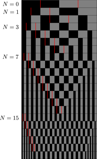
Now that we know which permutations can produce the maximal number of new colored segments, the question is where the cuts need to be located within the black and gray segments to achieve optimal mixing, such that each segment in the final state has the same length. Consider the case and ; at each iteration we cut the first black segment in half and the first gray segment in half at cut locations , as shown in Fig. 5(a). By Proposition 2.1 and the proof of Proposition 2.4, the maximum number, , new segments will be created at each iteration. However, the colored segments will not have equal lengths, so the protocol does not mix optimally. This can be overcome by rescaling the segments after a desired number of iterations so that they all have the same length, and then iterating backward to find where the cuts need to be located. In this case, the rescaling occurs between the bottom rows of Fig. 5(a,b), and by iterating backward (upward) in Fig. 5(b), the optimal cut locations are found, such that at . This rescaling procedure can be repeated for any variable IET, and so cut locations that achieve can be found for any variable IET that satisfies Proposition 2.1.
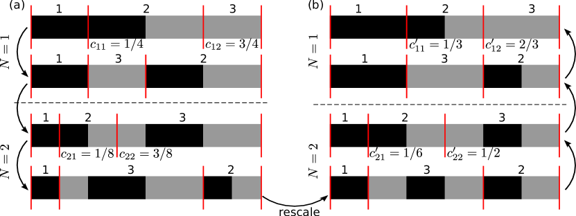
Cutting the first black segment and first gray segment at each iteration, as in Fig. 5, gives one optimal mixing protocol, but there are many more. For instance, before cutting at , there are two black segments and two gray segments. Instead of performing the cuts in the first black and first gray segments, we can also achieve optimal mixing by cutting in the first black segment and in the second gray segment [Fig. 4(c)], or in the second black segment and in the second gray segment [Fig. 4(d)]. As long as the first cut is in a black segment and the second cut is in a gray segment to its right, then optimal mixing will be achieved. We code the different optima as pairs , where represents which black segment is cut (e.g. if the first black segment is cut) and represents which gray segment is cut (e.g. if the second gray segment is cut). At the -th iteration, there are black segments and gray segments, so . Hence, at the -th iteration, there are distinct pairs of optimal cut locations, where denotes the binomial coefficient. Over the full iterations, the total number of distinct sets of optimal cut locations equals
| (11) |
This same approach can be used to find optimal mixing protocols for arbitrary numbers of iterations, , and cut pieces, . At the -th iteration, there are total segments, half black and half gray. Assuming the first segment is always black (or re-coloring as needed), and that the first cuts are always within black segments, and the final cuts are within gray segments, then by the proof of Proposition 2.4, optimal mixing () is guaranteed (after rescaling segment lengths). Like in the case above, we code the optimal cut locations by -tuples , where the ’s represent which black segments are cut (e.g., means the third cut occurs in the second black segment), and the ’s represent which gray segments are cut (e.g., means the fifth gray segment cut occurs in the third gray segment). Since the cuts in black segments must come first, the ’s and ’s satisfy , and hence there are possibilities. However, in some cases there are even more optima, because it is not always necessary to perform the first cuts within black segments and the final cuts within gray segments. For example, for variable IETs using the permutation , it can be shown that after the first iteration we can achieve optimal mixing by locating the cuts in the order black, black, gray, gray (BBGG) as described above; or the orders BGGB, GBBG, and GGBB. The orders BGBG and GBGB cannot produce optimal mixing (see Appendix A for full details). In the case with permutation , the first cut must always be in a black segment and the second in a gray segment. Hence, Eq. 11 accounts for all possibilities (Appendix A).
2.3 Extension to more than two colors
What is important is that we have a formulaic approach to find variable IETs that produce optimal mixing. Even though most of the results in this section use a two-color initial condition, many of the ideas can be extended to initial conditions with more colors. The main challenge when extending to more than two colors is that the metrics and are not equivalent. Optimal mixing is not simply a matter of producing the maximal number of segments like in the two-color case; the ordering of the colored segments is equally important to minimize . Therefore, it is more difficult to find necessary conditions for mixing to be optimal. However, it is relatively easy to find permutations and cut locations that produce optimal mixing for more than two colors. We follow essentially the same construction as the two-color case. For colors, , must be a multiple of in order to produce the same number of each colored segment at each iteration (equivalent to the condition that must be odd in Proposition 2.8). In the first iteration, we make cuts within each of the segments (like Proposition 2.8). For the permutation , we choose (Proposition 2.6 is valid for any number of colors), so that after rearranging, the first colored segment is still color . Then, through trial-and-error or solving a system of linear equations with the colors of the left and right edges of cut pieces as variables (see Appendix A), we find the permutations that yield the sequence repeated times, i.e. those permutations that yield new sequences of the colors. This is equivalent to repeating the black-gray pair for the two-color case. In successive iterations, as long as cut segments have the same colors as in the first iteration (i.e. the first cuts are within segments with color , the next cuts are within segments with color , and so on), then the IET will yield the sequence repeated times, where is the number of iterations. We then use the same rescaling process demonstrated in Fig. 5 to find cut locations such that all the segments have the same length after a desired number of iterations, which means the IET mixes optimally, i.e. .
Consider the three-color initial condition () in Fig. 6. To produce optimal mixing, must be a multiple of . For , one cut is made within each of the black, gray and white segments, as shown in the top row of Fig. 6(a). We assume that , so that after rearrangement by , the first piece, , does not move. Since has a black right edge, to obtain the sequence black-gray-white repeated times, the next piece must have a gray left edge, meaning it must be . Now, the right edge of is white, so the next piece must have a black left edge, meaning it must be . Lastly, the fourth piece, , remains in place. Therefore, the permutation yields two repeating black-gray-white sequences. In subsequent iterations, the sequence black-gray-white will be repeated times as long as the first cut is within a black segment, the second cut is within a gray segment, and the third cut is within a white segment. This is demonstrated in Fig. 6(a), where the cuts are made at the midpoints of the first black, gray and white segments. However, for in Fig. 6(a), mixing is suboptimal because the segment lengths are unequal. Optimal cut locations are found using the same rescaling process demonstrated in Fig. 5, i.e. segments in the bottom row of Fig. 6(a) are rescaled to obtain the bottom row of Fig. 6(b), then the IET is iterated backward.
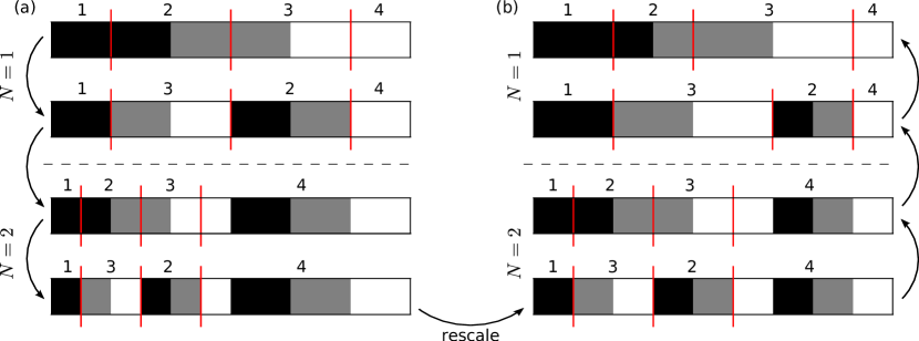
The above approach provides a relatively easy way to find permutations and cut locations that mix optimally for any number of colors. In fact, the permutations found using this approach are the only permutations that can mix optimally. The only permutations that this method would not capture are those that permute the repeating sequence of colors, for instance changing from repeating black-gray-white to repeating black-white-gray. Consider the first iteration, , in Fig. 6(a), and suppose that the repeating sequence of colors changed from black-gray-white to black-white-gray. Since the piece has a black left edge, after rearrangement it must be preceded by a piece with a gray right edge, meaning it must be preceded by . However, followed by results in the sequence black-gray-black, and so colors cannot be evenly distributed along the line (each pair of black segments must have a gray segment and a white segment between them). Therefore, for the case with three colors and , the repeating sequence of colors must remain black-gray-white.
More generally, since cuts must occur within the colored segments, in the first iteration there must be cut pieces that each have exactly two colors, on the left and on the right, for . For example, with three colors (black-gray-white), there must be a black-gray piece and a gray-white piece ( and at each iteration in Fig. 6). For an optimally mixing permutation, after the first iteration (and every iteration) each set of colored segments must have one of each color (evenly distributed colors), and so the same sequence of colors must repeat itself, where is a permutation of . Assuming (we can always start with the first color in the initial condition), there is a cut piece with two colors, on the left and on the right, so must always follow , and . Similarly, there is a cut piece with on the left and on the right, so must always follow , and . Continuing this process for all the pieces with two colors yields for all , i.e. the ordering of the colors cannot change, and so our method captures all optimally mixing permutations.
Now that we know how to find optimally mixing variable IETs, the question is: How much better is the mixing they produce compared to fixed IETs?
3 Variable vs. fixed cutting-and-shuffling
Intuitively, the added parametric freedom of variable protocols should enable significantly improved mixing. In this section we compare mixing produced by optimal variable IETs, like those discussed in the previous section, with mixing produced by fixed IETs with random cut locations and fixed IETs with optimally chosen cut locations. Considering two, three, and four colors in the initial condition, we show that in all cases optimal variable IETs produce significantly better mixing than random fixed IETs and that the degree of improvement increases with the number of iterations, . Furthermore, with more colors in the initial condition, optimal variable IETs improve mixing more than both random and optimal fixed IETs.
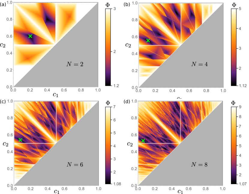
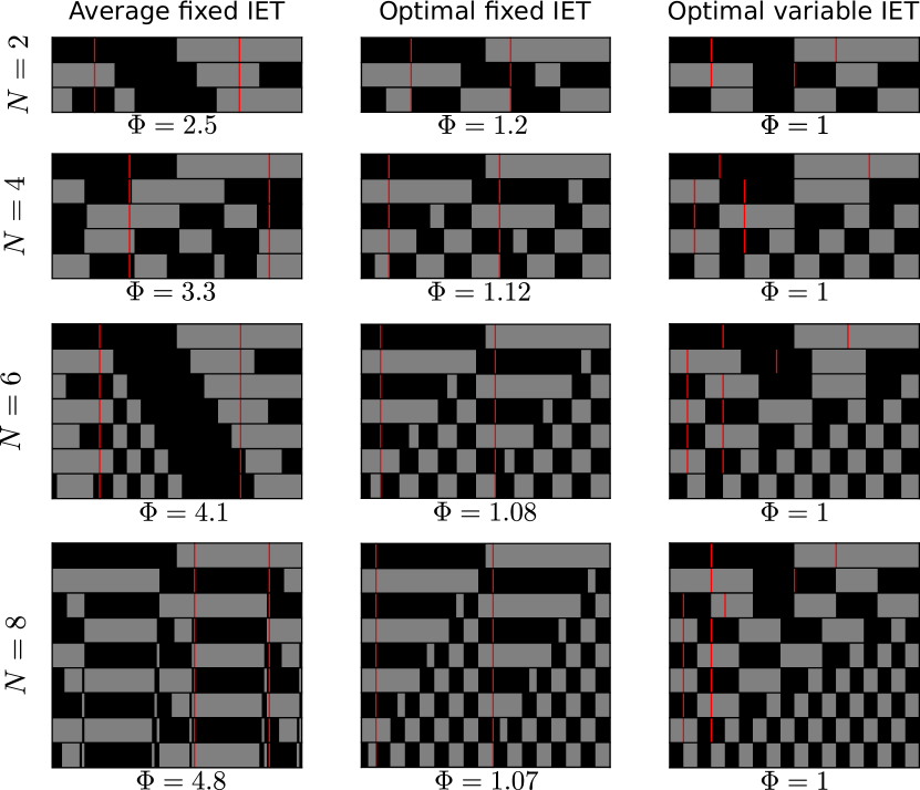
First, consider mixing the two-color initial condition in the top row of the space-time plot in Fig. 5. For permutations with , from Proposition 2.1 there are only three permutations that can achieve optimal mixing in the variable case, , , and . The permutations and are both reducible, and hence do not mix in the fixed case (the IET is periodic with period equal to two). On the other hand, the permutation is irreducible, and hence can at least achieve weak-mixing in the fixed case (when the two cut locations are chosen to satisfy the Keane minimality condition). However, weak-mixing only guarantees mixing over infinite iterations, and we are more interested in optimizing mixing over finite numbers of iterations. For fixed IETs with permutation , we calculate across the cut location parameter space, , (sampling on a grid with a spacing of in each direction) The results are shown in Fig. 7 for , , , and iterations, with the darkest color intensity indicating the value of the mixing metric closest to the optimum of . The average value of , , across the parameter space is the expected, or “typical,” degree of mixing for randomly chosen fixed cut locations. As the number of iterations increases, grows approximately linearly, shown by the dotted black curve in Fig. 8(a). This means that on average, the mixing quality, compared to the variable optimum (), becomes worse as the number of iterations increases. To show a typical space-time plot for an average fixed IET, we arbitrarily select a particular IET such that for each , which is shown in the first column of Fig. 9. As increases, there is a small improvement in mixing, i.e. there are more black and gray segments, and the length of the longest colored segment, , decreases. However, the colored segments vary substantially in their lengths. Therefore, for the average “typical” fixed IET, the mixing metric , which is normalized by the optimal variable IET, increases rapidly as increases. In contrast, for the optimal variable IETs (third column of Fig. 9), the number of segments grows faster [as ], and decreases more rapidly [as ], indicating all segments have uniform length.
Now we compare optimal variable IETs to optimal fixed IETs, again with the two-color initial condition and . Optimal fixed IETs are found for each by progressively refining the sample grid in the parameter space around a minimum value of , , shown as green ‘’s in Fig. 7.†††Due to symmetry of the parameters about the line there are two minima. We find the one such that . For the two-color initial condition, in contrast to the average, remains close to [dotted black curve in Fig. 8(b)], indicating that the optimal fixed IET mixes almost as well as the optimal variable IET. This is demonstrated in the second column of Fig. 9. The optimal fixed IETs (second column) yield the maximum number of segments, , and the segments are relatively uniform, with the uniformity of the segments improving with . As a result, approaches as increases.
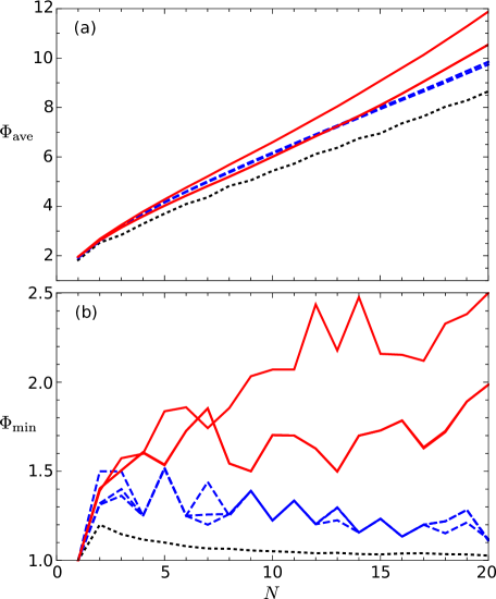
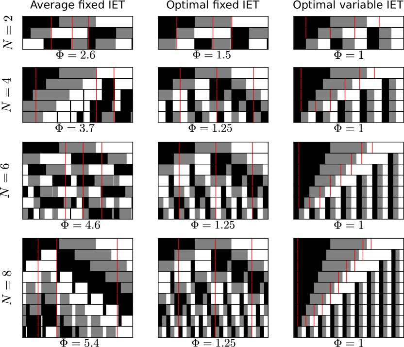
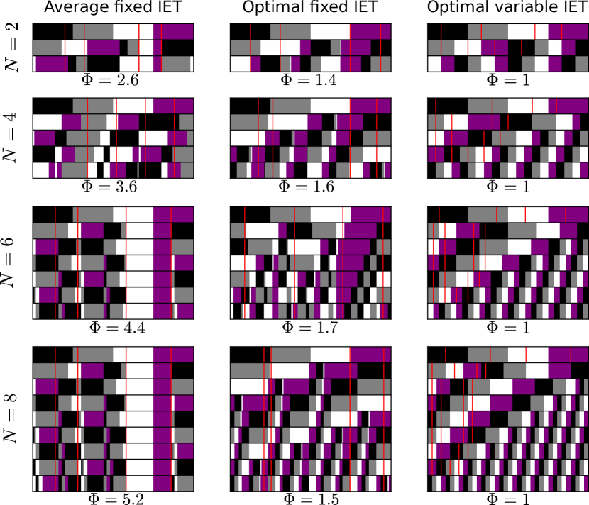
We perform similar analyses for three-color and four-color initial conditions. As discussed in Section 2.3, for the three-color initial condition, must be a multiple of three to achieve optimal mixing. Thus, is the minimum permutation length. In this case, the only permutations that can achieve optimal mixing are the rotations of , of these three are irreducible, namely , , and . Similarly, for the four-color initial condition, must be a multiple of four to achieve optimal mixing. For , the only permutations that can achieve optimal mixing are the rotations of , of these three are irreducible, namely , , and . For each initial condition, each irreducible permutation, and each , we find the average, , and minimum, , values of for fixed IETs by sampling the parameter space , similar to the approach to generate Fig. 7 for two colors and . As with the two-color initial condition, grows approximately linearly as increases for both the three-color [dashed blue curves in Fig. 8(a), all three curves overlap] and four-color [solid red curves in Fig. 8(a), two of the three curves overlap due to a reflection symmetry] initial conditions, meaning mixing using random fixed cuts, compared to the variable optimum (), becomes progressively worse as increases. This is demonstrated in the space-time plots for fixed IETs with in the first columns of Figs. 10 and 11. As increases, the number of segments increases, the length of the longest segment decreases, and the colors become more evenly distributed along the line, indicating improved mixing. However, when compared to the optimal variable IETs (third columns of Figs. 10 and 11) it is clear that at each , the average fixed IETs, have fewer segments, the segments are longer, and the colors are not as evenly distributed, leading to large values of . Since the discrepancy in mixing quality between average fixed IETs and optimal variable IETs becomes greater as increases, increases with [Fig. 8(a)].
Comparing for the different initial conditions, Fig. 8(a) shows that when , is greater when there are more colors in the initial condition (the curves are ordered vertically according to the number of colors in the initial condition). This means that when there are more colors in the initial condition, mixing using random fixed cut locations becomes worse relative to the optimum (). The same vertical ordering of curves occurs when considering optimal fixed IETs (those with ) as well, shown in Fig. 8(b). Therefore, when there are more colors in the initial condition, mixing using optimal fixed cut locations also becomes worse relative to the optimum (). While the optimal fixed IETs for the two-color initial condition could achieve near optimal values of , the optimal fixed IETs for the three-color and four-color initial conditions perform significantly worse. This is demonstrated by the space-time plots for optimal fixed IETs in the second columns of Figs. 10 and 11. In each case the maximum number of segments is created, but they are not quite equal in length, and, more importantly, the colors are not evenly distributed.
To summarize, increasing complexity in the initial condition (more colors) results in increased improvement in the mixing quality achieved by optimal variable IETs compared to both random fixed IETs and optimal fixed IETs. A simple explanation for this behavior is that there are more competing interests, i.e. competition between equal segment lengths and even distribution of the colors, when there are more colors in the initial condition. With more colors it becomes increasingly difficult to maintain a repeating fixed order of the colored segments without moving the cut locations. Using variable IETs overcomes these limitations in fixed IETs.
4 Strategies for cutting-and-shuffling over many iterations in general systems
While optima can be found analytically for variable IETs with simple initial conditions for arbitrary numbers of iterations, more complex cutting-and-shuffling systems require computationally expensive numerical optimization methods. For variable systems, this computational expense is compounded because the number of control parameters grows linearly with the number of iterations. In typical mixing problems, it is desired to optimize mixing over a small number of iterations, where numerical optimization methods are feasible. However, there may be situations where it is not possible to reach the desired mixing quality in a small number of iterations, and optimization over the required number of iterations is computationally prohibitive.
Even for fixed protocols, where the number of control parameters does not grow with the number of iterations, the distribution of the mixing metric across the parameter space is likely to be multi-modal, discontinuous, and complex, as demonstrated in Fig. 7(d) for the relatively simple case with the two-color initial condition, , and only 8 iterations. This complexity generally increases with the number of iterations, making finding optima more challenging, as higher resolutions in the initial search grid are required.
There are other general strategies for optimizing mixing over a large number of iterations that can be used for cutting-and-shuffling systems. The first is to use geometric properties of the piecewise isometry. For IETs, the Keane minimality condition can be used to predict long-term mixing quality: a fixed IET will be ergodic provided the permutation is irreducible and not a rotation, and the lengths of the cut pieces are rationally independent [18, 43]. Furthermore, fixed IETs satisfying the Keane minimality condition are almost always weak-mixing [2], which is a stronger sense of mixing than ergodicity [41]. Krotter et al. [21] extended this work to find conditions for protocols to achieve good mixing in a finite time. These weak-mixing fixed IETs, while not optimal, can achieve good mixing over large numbers of iterations, i.e. in the limit of infinitely many iterations the domain will be completely homogenized.
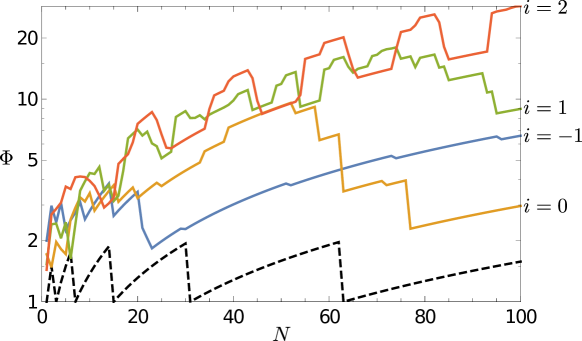
To explore this further, we use the same IET formulation as Krotter et al., which is demonstrated in Fig. 1. An irreducible permutation is chosen that is not a rotation, and a ratio of successive cut piece lengths, , is chosen that determines the lengths of the cut pieces. For example, in Fig. 1 the irreducible permutation is used in all three examples, is used in Fig. 1(a,b), and is used in Fig. 1(c). Here we examine this fixed IET approach over a large number of iterations for the two-color initial condition with a simpler irreducible permutation . We compare ratios for , such that is irrational, and so the IET satisfies the Keane minimality condition. The dependence of the mixing metric on for these cases is shown in Fig. 12 (note the logarithmic scale of the vertical axis). Some of these examples produce relatively good mixing, with at , but for others, is quite large, indicating poor mixing compared to the variable optimum ().
A similar strategy can be employed for 2D fixed PWIs using the exceptional set (where cuts occur), which is an intrinsic structure associated with 2D fixed PWIs. It has been shown that the area of the exceptional set can be used to predict the long-term mixing quality produced by 2D fixed PWIs [27]. Hence, long-term mixing can be improved by finding protocols that maximize the area of the exceptional set [34]. As for IETs, over finitely many iterations this approach would likely yield poor mixing compared to the variable optimum.
Another strategy for mixing over large numbers of iterations is to optimize over short time-horizons, i.e. optimizing for every iterations, where is much smaller than the total number of iterations . This strategy has proven effective for optimizing mixing in time-dependent fluid flows [6]. In many practical applications, the difference between the optima obtained from short time-horizon optimization and the global optimum is likely to be insignificant.
To demonstrate the effectiveness of short time-horizon optimization, we consider variable IETs with a time-horizon , i.e. we optimize mixing at each iteration separately. The result is the ad hoc method described briefly at the end of Section 2.1, where the longest segments of each distinct color are cut in half at each iteration. For example, in the two-color case with permutation (two cuts within the domain), the longest black and longest gray segments are cut in half at each iteration, as shown in Fig. 3. If there are multiple segments that all have the longest length, then we can arbitrarily choose which one to cut. In Fig. 3, the cut is made in the first maximal black segment and in the first maximal gray segment when there are multiple segments that share the longest length. This ad hoc approach is computationally inexpensive, and has a number of advantages compared to fixed IETs. First, this approach achieves optimal mixing () whenever , corresponding to points in Fig. 12 where the dashed black curve touches the horizontal axis. Also, the worst mixing (maxima of ) occurs at the iterations , and it can be shown that at these iterates , so for all . Thus, the ad hoc approach mixes significantly better than the weak-mixing protocols considered in Fig. 12. The key is that for fixed IETs, even weak-mixing ones, segments of the same color frequently reassemble. This means that the number of segments is generally significantly lower than the maximum, , that can be achieved by optimal variable IETs. On the other hand, reassembly of same-colored segments never occurs using the ad hoc method, so the maximal number of segments is always achieved. The only limitation is that the segments do not have equal lengths.
Another advantage of the ad hoc method, compared to both fixed IETs and optimal variable IETs, is that it is adaptive, i.e. it accounts for the current state of the scalar field. This means that if cuts are imprecise, as has been considered for fixed IETs like those in Fig. 1 [45], the method can correct itself and not compound the error.
Therefore, the ad hoc method provides a good alternative for mixing when the required number of iterations is large and finding optima for the total number of iterations is computationally prohibitive. Similar heuristics could be used for more general cutting-and-shuffling systems, such that cuts are located to bisect the largest unmixed regions.
5 Conclusions
Variable cutting-and-shuffling strategies allow for significantly improved mixing compared to fixed cutting-and-shuffling. We have identified optimal variable cutting-and-shuffling strategies for IETs with an initial condition consisting of a number of differently colored segments, and we have shown that these optimal variable IETs can produce significantly better mixing than general fixed IETs. Furthermore, the improvement in mixing quality increases with the number of colors in the initial condition. This is because when there are more colors it is more difficult to satisfy the two competing interests: small colored segments and evenly distributed colors.
For more general systems with cutting-and-shuffling, optimizing mixing over large numbers of iterations, or when there are many cuts per iteration, is generally computationally prohibitive. This is especially true for variable strategies, where the number of control parameters increases linearly with the number of iterations. We demonstrate that an ad hoc adaptive method, cutting the largest unmixed regions in half, provides a computationally inexpensive alternative. For IETs, this ad hoc method is equivalent to optimizing using a one-iteration time-horizon, and yields significantly better mixing than examples of weak-mixing fixed IETs. Using the ad hoc method, the mixing metric is guaranteed to be within a constant factor of the optimum, for any number of iterations. The key to the success of the ad hoc method is that segments of the same color never reassemble, meaning the maximum number of segments and interfaces will always be created. The adaptive nature of the ad hoc method also means that it self corrects for any inexactness in the cut locations [45], or inexactness in the initial condition.
A key assumption when finding optimal mixing protocols is that the initial condition is known exactly. However, in many applications, the initial condition is not known exactly, but rather has a probability distribution. If the mixing quality is highly sensitive to the initial condition, then the optimal mixing protocol for a specific initial condition is irrelevant since this initial condition, or any other specific initial condition, may be unattainable in practice. In this case, it is more desirable to use a protocol that is optimal over a distribution of potential initial conditions. Future work should focus on this problem, developing strategies to optimize mixing when the initial condition has a probability distribution. This could be achieved by replacing the mixing metric with a weighted mean of the metric over the distribution of possible initial conditions. A yet more general approach could be to optimize mixing in a way that is entirely independent of the initial condition, for instance optimizing properties of the map itself. For example, maximizing the eigenvalues of the transfer operator in fluid flows maximizes the decay rate of any concentration field toward the uniform distribution [11].
Another important question is how best to optimize mixing in more general variable systems with cutting-and-shuffling, including 2D piecewise isometries (PWIs) [33, 32, 12, 28, 27, 16, 34], and systems with cutting-and-shuffling combined with stretching-and-folding and/or diffusion [1, 39, 20, 10, 38, 35, 37, 36]. The added complexity means that exact methods like those in Section 2.2 are unlikely to be possible, but numerical and heuristic optimization strategies could be developed. For example, symmetries could be used to systematically destroy non-mixing regions [8, 9].
Appendix A Color orders for cuts in optimal variable IETs
Consider the two-color initial condition, and a variable IET with permutation and . For to produce the maximal number of new segments, in the first iteration one cut must be located within the black segment, and one cut located within the gray segment, as shown in Fig. 4(a). Otherwise there would be an imbalance in the number of black and gray left and right edges of cut pieces. We also show in Section 2.2 that in subsequent iterations, the maximum number of new segments will be created if we choose the first cut within a black segment and the second cut within a gray segment. However, it is not clear that this is the only choice that will work. What if we choose the first cut to be located within a gray segment, and the second cut located within a black segment? Consider the second iteration, where before cutting-and-shuffling the line, there are two black segments and two gray segments [Fig. 4(b–e)]. Let denote the colors of the left edges of the cut pieces, and denote the colors of the right edges, as shown in Fig. 4(b–e). Here we use to represent black and to represent gray. We know that because the left edge of the line is black, and because the right end of the line is gray. We show in Section 2.2 that for optimal variable IETs, cuts must occur within segments, which translates to
| (12) |
After rearrangement, each black edge must join with a gray edge, which is expressed as
| (13) |
Combining Eq. 12, Eq. 13, and the conditions and , we have a linear system of equations for the variables , . Substituting Eq. 12 into Eq. 13 and using , we reduce the system of equations to
| (14) |
for , so that and are the only two variables. Substituting into Eq. 14, we obtain
| (15) | ||||
where each equation is modulo . This has the unique solution , . Hence, the first cut must occur within a black segment, and the second cut must occur within a gray segment. There are no other possibilities that will yield optimal mixing. Furthermore, Eq. 12–Appendix A hold for all , just replace with and with , and so the first cut must always occur within a black segment, and the second cut within a gray segment.
Following the same procedure as above, Eq. 14 must be satisfied for any variable IET that produces optimal mixing. We discuss two cases with . First, let , which satisfies Proposition 2.1, and so can produce optimal mixing. Substituting into Eq. 14, we obtain
| (16) | ||||
where each equation is modulo . In addition, because the right edge of the line must always be gray, since the left edge is always black []. The system specified by Appendix A has the unique solution , , which means the first two cuts must always occur within black segments, and the last two cuts must always occur within gray segments.
Now consider . Substituting into Eq. 14, we obtain
| (17) | ||||
where each equation is modulo . Note that the first and third equations are equivalent, as are the second and fourth. In addition, the last equation provides no new information. We already know that because the right edge of the line must always be gray, since the left edge is always black []. Therefore, for the unknown variables we effectively have only two equations. The color at the first cut must be opposite to the color at the third cut, and likewise for the second and fourth cuts, but we are free to choose the colors of the third and fourth cuts. Hence there are four possible solutions:
| (18) | ||||
which means that at each iteration cuts can occur in the order gray, gray, black, black (GGBB), GBBG, BGGB, or BBGG, respectively. Therefore, there are many more optimal variable IETs that use the permutation compared to the permutation .
This approach can be repeated for any permutation that satisfies Proposition 2.1, and can also be extended to initial conditions with colors by simply changing Eq. 13 to be modulo .
References
- [1] P. Ashwin, M. Nicol, and N. Kirkby, Acceleration of one-dimensional mixing by discontinuous mappings, Physica A, 310 (2002), pp. 347 – 363, https://doi.org/10.1016/S0378-4371(02)00774-4.
- [2] A. Avila and G. Forni, Weak mixing for interval exchange transformations and translation flows, Ann. Math., (2007), pp. 637–664, http://www.jstor.org/stable/20160038.
- [3] J. Boujlel, F. Pigeonneau, E. Gouillart, and P. Jop, Rate of chaotic mixing in localized flows, Phys. Rev. Fluids, 1 (2016), p. 031301, https://doi.org/10.1103/PhysRevFluids.1.031301.
- [4] I. C. Christov, R. M. Lueptow, and J. M. Ottino, Stretching and folding versus cutting and shuffling: An illustrated perspective on mixing and deformations of continua, Am. J. Phys., 79 (2011), pp. 359–367, https://doi.org/10.1119/1.3533213.
- [5] I. C. Christov, R. M. Lueptow, J. M. Ottino, and R. Sturman, A study in three-dimensional chaotic dynamics: Granular flow and transport in a bi-axial spherical tumbler, SIAM J. Appl. Dyn. Syst., 13 (2014), pp. 901–943, https://doi.org/10.1137/130934076.
- [6] L. Cortelezzi, A. Adrover, and M. Giona, Feasibility, efficiency and transportability of short-horizon optimal mixing protocols, J. Fluid Mech., 597 (2008), p. 199–231, https://doi.org/10.1017/S0022112007009676.
- [7] P. V. Danckwerts, The definition and measurement of some characteristics of mixtures, Appl. Sci. Res., 3 (1952), pp. 279–296, https://doi.org/10.1007/BF03184936.
- [8] J. G. Franjione, C. Leong, and J. M. Ottino, Symmetries within chaos: A route to effective mixing, Phys. Fluids A-Fluid, 1 (1989), pp. 1772–1783, https://doi.org/10.1063/1.857504.
- [9] J. G. Franjione and J. M. Ottino, Symmetry concepts for the geometric analysis of mixing flows, Philos. T. Roy. Soc. A, 338 (1992), pp. 301–323, https://doi.org/10.1098/rsta.1992.0010.
- [10] G. Froyland, C. González-Tokman, and T. M. Watson, Optimal mixing enhancement by local perturbation, SIAM Rev., 58 (2016), pp. 494–513, https://doi.org/10.1137/15M1023221.
- [11] G. Froyland and N. Santitissadeekorn, Optimal mixing enhancement, SIAM J. Appl. Math., 77 (2017), pp. 1444–1470, https://doi.org/10.1137/16M1091496.
- [12] H. Haller, Rectangle exchange transformations, Monatsh. Math., 91 (1981), pp. 215–232, https://doi.org/10.1007/BF01301789.
- [13] T. P. Hunt, D. Issadore, and R. M. Westervelt, Integrated circuit/microfluidic chip to programmably trap and move cells and droplets with dielectrophoresis, Lab. Chip, 8 (2008), pp. 81–87, https://doi.org/10.1039/B710928H.
- [14] S. W. Jones and H. Aref, Chaotic advection in pulsed source-sink systems, Phys. Fluids, 31 (1988), pp. 469–485, https://doi.org/10.1063/1.866828.
- [15] G. Juarez, I. C. Christov, J. M. Ottino, and R. M. Lueptow, Mixing by cutting and shuffling 3D granular flow in spherical tumblers, Chem. Eng. Sci., 73 (2012), pp. 195 – 207, https://doi.org/10.1016/j.ces.2012.01.044.
- [16] G. Juarez, R. M. Lueptow, J. M. Ottino, R. Sturman, and S. Wiggins, Mixing by cutting and shuffling, Europhys. Lett., 91 (2010), p. 20003, http://stacks.iop.org/0295-5075/91/i=2/a=20003.
- [17] A. Katok, Interval exchange transformations and some special flows are not mixing, Isr. J. Math., 35 (1980), pp. 301–310, https://doi.org/10.1007/BF02760655.
- [18] M. Keane, Interval exchange transformations, Math. Z., 141 (1975), pp. 25–31, https://doi.org/10.1007/BF01236981.
- [19] M. Keane, Non-ergodic interval exchange transformations, Isr. J. Math., 26 (1977), pp. 188–196, https://doi.org/10.1007/BF03007668.
- [20] H. Kreczak, R. Sturman, and M. C. T. Wilson, Deceleration of one-dimensional mixing by discontinuous mappings, Phys. Rev. E, 96 (2017), p. 053112, https://doi.org/10.1103/PhysRevE.96.053112.
- [21] M. K. Krotter, I. C. Christov, J. M. Ottino, and R. M. Lueptow, Cutting and shuffling a line segment: mixing by interval exchange transformations, Int. J. Bifurcat. Chaos, 22 (2012), p. 1230041, https://doi.org/10.1142/S0218127412300418.
- [22] C. W. Leong and J. M. Ottino, Experiments on mixing due to chaotic advection in a cavity, J. Fluid Mech., 209 (1989), pp. 463–499, https://doi.org/10.1017/S0022112089003186.
- [23] H. Masur, Interval exchange transformations and measured foliations, Ann. Math., 115 (1982), pp. 169–200, https://doi.org/10.2307/1971341.
- [24] G. Mathew, I. Mezić, S. Grivopoulos, U. Vaidya, and L. Petzold, Optimal control of mixing in stokes fluid flows, J. Fluid Mech., 580 (2007), p. 261–281, https://doi.org/10.1017/S0022112007005332.
- [25] G. Mathew, I. Mezić, and L. Petzold, A multiscale measure for mixing, Physica D, 211 (2005), pp. 23–46, https://doi.org/10.1016/j.physd.2005.07.017.
- [26] R. A. Mitchell and J. D. Meiss, Designing a finite-time mixer: Optimizing stirring for two-dimensional maps, SIAM J. Appl. Dyn. Syst., 16 (2017), pp. 1514–1542, https://doi.org/10.1137/16M1107139.
- [27] P. P. Park, T. F. Lynn, P. B. Umbanhowar, J. M. Ottino, and R. M. Lueptow, Mixing and the fractal geometry of piecewise isometries, Phys. Rev. E, 95 (2017), p. 042208, https://doi.org/10.1103/PhysRevE.95.042208.
- [28] P. P. Park, P. B. Umbanhowar, J. M. Ottino, and R. M. Lueptow, Mixing with piecewise isometries on a hemispherical shell, Chaos, 26 (2016), 073115, p. 073115, https://doi.org/10.1063/1.4955082.
- [29] B. Rallabandi, C. Wang, and S. Hilgenfeldt, Analysis of optimal mixing in open-flow mixers with time-modulated vortex arrays, Phys. Rev. Fluids, 2 (2017), p. 064501, https://doi.org/10.1103/PhysRevFluids.2.064501.
- [30] F. Schönfeld, V. Hessel, and C. Hofmann, An optimised split-and-recombine micro-mixer with uniform ‘chaotic’mixing, Lab. Chip, 4 (2004), pp. 65–69, https://doi.org/10.1039/B310802C.
- [31] A. Schultz, I. Papautsky, and J. Heikenfeld, Investigation of Laplace Barriers for Arrayed Electrowetting Lab-on-a-Chip, Langmuir, 30 (2014), pp. 5349–5356, https://doi.org/10.1021/la500314v.
- [32] A. Scott, Hamiltonian mappings and circle packing phase spaces: numerical investigations, Physica D, 181 (2003), pp. 45 – 52, https://doi.org/10.1016/S0167-2789(03)00095-2.
- [33] A. Scott, C. Holmes, and G. Milburn, Hamiltonian mappings and circle packing phase spaces, Physica D, 155 (2001), pp. 34 – 50, https://doi.org/10.1016/S0167-2789(01)00263-9.
- [34] L. D. Smith, P. P. Park, P. B. Umbanhowar, J. M. Ottino, and R. M. Lueptow, Predicting mixing via resonances: Application to spherical piecewise isometries, Phys. Rev. E, 95 (2017), p. 062210, https://doi.org/10.1103/PhysRevE.95.062210.
- [35] L. D. Smith, M. Rudman, D. R. Lester, and G. Metcalfe, Mixing of discontinuously deforming media, Chaos, 26 (2016), p. 023113, https://doi.org/10.1063/1.4941851.
- [36] L. D. Smith, M. Rudman, D. R. Lester, and G. Metcalfe, Impact of discontinuous deformation upon the rate of chaotic mixing, Phys. Rev. E, 95 (2017), p. 022213, https://doi.org/10.1103/PhysRevE.95.022213.
- [37] L. D. Smith, M. Rudman, D. R. Lester, and G. Metcalfe, Localized shear generates three-dimensional transport, Chaos, 27 (2017), p. 043102, https://doi.org/10.1063/1.4979666.
- [38] L. D. Smith, P. B. Umbanhowar, J. M. Ottino, and R. M. Lueptow, Mixing and transport from combined stretching-and-folding and cutting-and-shuffling, Phys. Rev. E, 96 (2017), p. 042213, https://doi.org/10.1103/PhysRevE.96.042213.
- [39] R. Sturman, The role of discontinuities in mixing, Adv. Appl. Mech., 45 (2012), pp. 51–90, https://doi.org/10.1016/B978-0-12-380876-9.00002-1.
- [40] R. Sturman, S. W. Meier, J. M. Ottino, and S. Wiggins, Linked twist map formalism in two and three dimensions applied to mixing in tumbled granular flows, J. Fluid Mech., 602 (2008), p. 129–174, https://doi.org/10.1017/S002211200800075X.
- [41] R. Sturman, J. M. Ottino, and S. Wiggins, The mathematical foundations of mixing: the linked twist map as a paradigm in applications: micro to macro, fluids to solids, Cambridge Monographs on Applied and Computational Mathematics (22), Cambridge University Press, 2006.
- [42] W. A. Veech, Interval exchange transformations, J. Anal. Math., 33 (1978), pp. 222–272, https://doi.org/10.1007/BF02790174.
- [43] M. Viana, Ergodic theory of interval exchange maps, Rev. Mat. Complut., 19 (2006), pp. 7–100, http://eudml.org/doc/40876.
- [44] A. Vikhansky, Enhancement of laminar mixing by optimal control methods, Chem. Eng. Sci., 57 (2002), pp. 2719 – 2725, https://doi.org/10.1016/S0009-2509(02)00122-7.
- [45] M. Yu, P. B. Umbanhowar, J. M. Ottino, and R. M. Lueptow, Cutting and shuffling of a line segment: Effect of variation in cut location, Int. J. Bifurcat. Chaos, 26 (2016), p. 1630038, https://doi.org/10.1142/S021812741630038X.
- [46] Z. Zaman, M. Yu, P. P. Park, P. B. Umbanhowar, J. M. Ottino, and R. M. Lueptow, Persistent structures in a 3D dynamical system with solid and fluid regions, arXiv preprint, arXiv:1706.00864.