A quartet of black holes and a missing duo: probing the low-end of the M relation with the adaptive optics assisted integral-field spectroscopy
Abstract
We present mass estimates of supermassive black holes in six nearby fast rotating early-type galaxies (NGC 4339, NGC 4434, NGC 4474, NGC 4551, NGC 4578 and NGC 4762) with effective stellar velocity dispersion around 100 km/s. We use near-infrared laser-guide adaptive optics observations with the GEMINI/NIFS to derive stellar kinematics in the galactic nuclei, and SAURON observations from the ATLAS3D Survey for large-scale kinematics. We build axisymmetric Jeans Anisotropic Models and axisymmetric Schwarzschild dynamical models. Both modelling approaches recover consistent orbital anisotropies and black hole masses within confidence level, except for one galaxy for which the difference is just above the level. Two black holes (NGC 4339 and NGC 4434) are amongst the largest outliers from the current black hole mass - velocity dispersion relation, with masses of and M⊙, respectively ( confidence level). The black holes in NGC 4578 and NGC 4762 lie on the scaling relation with masses of and M⊙, respectively ( confidence level). For two galaxies (NGC 4474 and NGC 4551) we are able to place upper limits on their black holes masses ( and M⊙, respectively, confidence level). The kinematics for these galaxies clearly indicate central velocity dispersion drops within a radius of 35 pc and 80 pc, respectively. These drops cannot be associated with cold stellar structures and our data do not have the resolution to exclude black holes with masses an order of magnitude smaller than the predictions. Parametrizing the orbital distribution in spherical coordinates, the vicinity of the black holes is characterized by isotropic or mildly tangential anisotropy.
keywords:
galaxies: individual: NGC 4339, NGC 4434, NGC 4474, NGC 4551, NGC 4578, NGC 4762 – galaxies: kinematics and dynamics – galaxies: supermassive black holes1 Introduction
Determining the masses of black holes in the centres of galaxies is marred with difficulties. Galaxies are systems with stars of different ages and metallicities, grouped in a number of structural components such as bulges, discs, rings, bars and spherical haloes. They also contain gas in various phases, and regions forming stars. Central black holes can be considered part of the invisible dark matter content of galaxies responsible for the changes to the total gravitational potential. All these components need to be taken into account at various levels of sophistication when constructing dynamical models and estimating masses of central black holes.
There are several established methods for measuring the black hole masses, which have one thing in common: the use of luminous tracers of the gravitational potential, such as stars or clouds of ionized or molecular gas. The observed motions of these tracers are used to constrain dynamical models, which can separate the contribution to the potential of the black hole and the rest of the galaxy, and, therefore, provide the black hole mass, MBH. The various approaches of using different types of tracers are reviewed in Kormendy & Ho (2013). For all types of dynamical models, and specifically for the stellar dynamical models used in the work presented here, it is essential that the assumed gravitational potential is a realistic representation of the galaxy, and that the data describing the motions of the tracer are adequate to distinguish the presence of a black hole(see for reviews Ferrarese & Ford, 2005; Kormendy & Ho, 2013).
The mass of a black hole is added as a component in the total gravitational potential defined by the distribution of stars and, possibly, dark matter (the mass of the gas in the type of systems considered here is usually small and typically ignored). It dominates a region defined as the sphere of influence (SoI), with a characteristic radius , where is the gravitational constant and is the characteristic velocity dispersion of the galaxy within an effective radius (de Zeeuw, 2001; Ferrarese & Ford, 2005). Within SoI, the black hole is the dominant source of the gravitational potential, but its influence can impact the galaxy at larger radii. The reason for this is that the gravitational potential falls off relatively slowly with , and that stars on non-circular orbits may pass within or close to the SoI, and therefore can be influenced by the black hole even though they spend most of their time well outside the SoI. This is why, to constrain a dynamical model, one needs to have good quality data covering the region close to the black hole, but also mapping the bulk of the galaxy body (e.g. Verolme et al., 2002).
The spectroscopic capabilities of the Hubble Space Telescope (HST) offered a way to probe the regions close to black holes at the high surface brightness centres of some galaxies (see fig. 1 of Kormendy & Ho, 2013), but it is the large collecting areas of the ground-based 8-10m telescopes assisted with natural guide star or laser guide star (LGS) adaptive optics (AO) that paved a way forward to extending the types of galaxies with measured black hole masses (e.g. Houghton et al., 2006; Häring-Neumayer et al., 2006; Nowak et al., 2007; Neumayer et al., 2007; Cappellari et al., 2009; Krajnović et al., 2009; McConnell et al., 2011; Walsh et al., 2012). To this one should add the opening of the wavelength space with the observations of the nuclear masers (e.g. Greene et al., 2010; Kuo et al., 2011; Greene et al., 2016) and the sub-millimetre interferometric observations of circumnuclear gas discs (e.g. Davis et al., 2013; Onishi et al., 2015; Barth et al., 2016). Regarding dynamical models based on stellar kinematics, the advent of mapping galaxy properties with integral-field unit (IFUs) spectrographs has greatly improved the observational constraints on stellar orbital structure (Krajnović et al., 2005), resulting in more secure determinations of MBH (Cappellari et al., 2010).
The price that has to be paid to determine a single MBH using stellar kinematics is, however, large: one typically needs observations coming from 3 to 4 different instruments usually mounted on the same number of different telescopes. These are the small-scale high-resolution IFU data [typically in the near-infrared (NIR) to increase the spatial resolution when observed from the ground], and the large scale IFU data of moderate (or poor) spatial resolution. These spectroscopic data are needed to determine the motions of the tracer, but imaging data are also needed to determine the spatial distribution of stars and infer the three-dimensional distribution of mass. Preferably, the imaging data should be of better spatial resolution than the spectroscopy, and currently the only source of such data is the HST. Large-scale (ground-based) imaging is also needed to map the stellar distribution (and ascertain the gravitational potential) to radii several times larger than the extent of the spectroscopic data.
Obtaining such data sets, and ensuring they are of uniform and sufficient quality, is not a small challenge. The hard-earned data sets accumulated by the community over the past several decades, revealed and confirmed with increasing confidence the striking correlations between the MBH and various properties of host galaxies. We refer the reader to in-depth descriptions and discussions on all black hole scaling relations in recent reviews by Ferrarese & Ford (2005), Kormendy & Ho (2013) and Graham (2016) and mention here only the M relation (Ferrarese & Merritt, 2000; Gebhardt et al., 2000). This relation, typically found to have the least scatter (e.g. Saglia et al., 2016; van den Bosch, 2016) reveals a close connection between two objects of very different sizes, implying a linked evolution of growth for both the host galaxy and its resident black hole.
Recent compilations provide lists of more than 80 dynamically determined MBH (e.g. Saglia et al., 2016), while the total number of black hole masses used in determining this relation approaches 200 (van den Bosch, 2016). Increases in sample size have shown that, contrary to initial expectation, the M relation shows evidence of intrinsic scatter (Gültekin et al., 2009b), and in particular that low- and high- regions have increased scatter (Hu, 2008; Graham & Li, 2009; McConnell & Ma, 2013). Low- and high-mass galaxies have different formation histories (e.g. Khochfar et al., 2011) and it is not surprising that their black holes might have different masses (Graham & Scott, 2013; Scott et al., 2013b), but as more black hole masses are gathered, there also seems to be a difference between galaxies of similar masses. On the high-mass side, brightest galaxies in cluster or groups seem to have more massive black holes than predicted by the relation (McConnell et al., 2011, 2012; Thomas et al., 2016), while among the low-mass systems, active galaxies, galaxies with bars or non-classical bulges show a large spread of MBH (Greene et al., 2010; Kormendy et al., 2011; Graham et al., 2011; Greene et al., 2016).
Determining the shape, scatter and extent of the M relation is important for our understanding of the galaxy evolution (see for a review Kormendy & Ho, 2013), growth of black holes, and their mutual connection. It is also crucial for calibrating the numerical simulations building virtual universes (e.g. Agarwal et al., 2014; Vogelsberger et al., 2014; Schaye et al., 2015), and every addition to the relation is still very valuable, especially when one considers that the MBH scaling relations are not representative of the general galaxy population (Lauer et al., 2007; Bernardi et al., 2007; Shankar et al., 2016).
In this paper we investigate six early-type galaxies (ETGs) belonging to the low velocity dispersion part of the M relation, and as a result add four more measurements to the scaling relations. For two additional galaxies we are not able to detect black holes, making them rather curious, but exciting exceptions to the expectation that all ETGs have central black holes. In Section 2 we define the sample, describe the observations, their quality and data reduction methods. In Section 3 we present the stellar kinematics used to constrain the dynamical models which are described in Section 4. Section 5 is devoted to the discussion on the results, in particular, the possible caveats in the construction of dynamical models, the location of our MBH with respect to other galaxies on the M relations, the internal orbital structure and the conjecture that two galaxies in our sample do not harbour black holes. We summarize our conclusions in Section 6. Appendices C, B, D and E present various material supporting the construction and validation of the dynamical models.
2 Sample selection, observations and data reduction
The core data set of this work was obtained using the Near-Infrared Integral Field Spectrograph (NIFS) on Gemini North Observatory on Hawaii and the SAURON111SAURON was decommissioned in 2016 and it was transferred to the Musèe des Confluences in Lyon where it is on display. IFU on the William Herschel Telescope of the Isaac Newton Group on La Palma. In addition to these spectroscopic observations we used images obtained with the Hubble Space Telescope (HST) and the Sloan Digital Sky Survey (SDSS).
2.1 Sample selection
Our goal was to obtain high spatial resolution kinematics of the nuclei of galaxies that have approximately km/s, probing the low mass end of the black hole scaling relations. The ATLAS3D sample (Cappellari et al., 2011a) was a unique data base from which to select these galaxies, as it provided the large-scale IFU observations and accurate estimates for a volume-limited sample of ETGs. However, not all low ATLAS3D galaxies could be included in the sample. The highest possible spatial resolution from the ground is achievable with an LGS AO system, which allows high spatial resolution observations of extended targets by relaxing the constraint for having a bright guide star close to the scientific target. However, a natural guide source is still required in order to correct for the so-called tip/tilt (bulk motion of the image) low-order distortion term, and to track the differential focus of the laser source (located in the atmospheric sodium layer at 90 km altitude, whose distance from the telescope changes with zenith distance) and the science target. In order to maximize the correction, the natural guide star should be relatively close to the target, and in the case of the GEMINI AO system Altair (Boccas et al., 2006) it can be as far as 25″ from the target and down to 18.5 mag in R band (in low sky background conditions). The ATLAS3D galaxies were not able to match even such relaxed restrictions. However, as the tip/tilt and focus corrections are also possible using the galaxy nucleus as the natural guide source provided there is a 1.5 mag drop within the central 1″, our targets were primarily selected to fulfil this requirement.
Further restrictions were imposed by considering the possible results of the dynamical models. A rule of thumb says that to provide constraints on the mass of the black hole in stellar dynamical models, one should resolve the black hole SoI. In Krajnović et al. (2009) we showed that it is possible to constrain the lower limit for the mass of a black hole even if the SoI is 2 – 3 times smaller than the nominal spatial resolution of the observations, provided one uses both the large-scale and high spatial resolution IFU data (see also Cappellari et al., 2010). This relaxation, nevertheless limits the number of possible galaxies as the SoI also decreases inversely with the distance of the galaxy. Selection based on SoI is only approximately robust as it relies on the choice of M scaling relation parameters, which are particularly uncertain in the low-mass regime. Our choice was to assume the Tremaine et al. (2002) relation, limited to galaxies with km/s and ″, yielding 44 galaxies222Note that the calculation was done on preliminary SAURON data and a number of values were different from the final published in Cappellari et al. (2013a) and used in the rest of the paper..
Additional restrictions were imposed to select only galaxies with archival HST imaging (in order to generate high resolution stellar mass models) and which showed no evidence of a bar (as bars introduce additional free parameters and degeneracies in the dynamical modelling). The combination of these considerations yielded a sample of 14 galaxies. Through several observing campaigns in 2009 and 2010 we obtained data for six galaxies: NGC 4339, NGC 4434, NGC 4474, NGC 4578 and NGC 4762. Table 1 presents the main properties of target galaxies and observational details.
Notes: Column 1: galaxy name; Column 2: effective (half-light) radius in arcsec; Column 3: velocity dispersion within the effective radius; Column 4: distance to the galaxy; Column 5: 2MASS K-band magnitude from Jarrett et al. (2000); Column 6: Bulge mass, obtained by multiplying the total dynamical mass from Cappellari et al. (2013b) and bulge-to-total ratio from Krajnović et al. (2013a); Column 7: assumed inclination. Column 8: Virgo membership. Distances are taken from Cappellari et al. (2011a), Virgo membership from Cappellari et al. (2011b), while all other properties are from Cappellari et al. (2013a).
2.2 Photometric data
Dynamical models depend on detailed parametrization of the stellar light distributions. Specifically, it is important to have high-resolution imaging of the central regions around the supermassive black hole, as well as deeper observations of the large radii. The former are important to describe the stellar potential close to the black hole, while the latter is critical for tracing the total stellar mass. The extent of the large-scale imaging should be such that it traces the vast majority of the stellar mass and we used the SDSS DR7 -band images (Abazajian et al., 2009), which were already assembled during the ATLAS3D Survey and are presented in (Scott et al., 2013a). The highest spatial resolution imaging was obtained using the HST archival data, using both the Wide-Field Planetary Camera (WFPC2, Holtzman et al., 1995) and Advanced Camera for Survey (ACS, Ford et al., 1998) cameras in filters most similar to the SDSS r-band (more details can be found in Table 2). Both WFPC2 and ACS calibrated data were requested through the ESA/HST Data Archive. The individual WFPC2 CR-SPLIT images were aligned and combined removing the cosmic rays. The ACS data were re-processed through the pyIRAF task multidrizzle.
2.3 Wide-field SAURON spectroscopy
The SAURON data were observed as part of the ATLAS3D Survey presented in Cappellari et al. (2011a), where the data reduction and the extraction of kinematics are also described. The velocity maps of our galaxies were already presented in Krajnović et al. (2011), while the higher order moments of the line-of-sight velocity distribution (LOSVD) are presented here in Appendix C. Observations of the ATLAS3D Survey were designed such that the SAURON field of view (FoV) covers at least one effective radius. For five of our galaxies a nominal SAURON FoV was sufficient, but in one case (NGC4762) the galaxy was covered with an adjacent mosaic of two SAURON footprints, resulting in approximately FoV. We use the SAURON kinematics available online333The data are available on the public ATLAS3D site: http://purl.org/atlas3d directly, with no modifications. More details on the instrument can be found in Bacon et al. (2001).
Notes: Column 1: galaxy name; Column 2: Gemini Proposal ID number; Column 3: total number of object exposures / total number of science exposures (object and sky); Column 4: total number of exposures merged into the final data cube; Column 5: total exposure time including both object and sky exposures (in hours); Column 6: HST proposal ID number; Column 7: HST Camera; and Column 8: filter.
2.4 NIFS LGS AO Spectroscopy
The small-scale, high spatial resolution IFU data were obtained using the NIFS (McGregor et al., 2003). All galaxies were observed in the K band with a H+K filter and a spectral resolution of . The observations were done in a O-S-O-O-S-O sequence, where O is an observation of the object (galaxy) and S is an observation of a sky field. NIFS pixels are rectangular () and we dithered the individual object frames by a non-integer number of pixels in both directions, to provide redundancy against bad detector pixels, and to oversample the point spread function (PSF). Each observation was for 600 s. In addition to galaxies, a set of two telluric stars were observed before and after the science observations, covering A0 V and G2 V types. Their observation followed the same strategy of object and sky interchange as for the science targets. A summary of the NIFS observations are given in Table 2.
The reduction of the NIFS data was identical to that described in Krajnović et al. (2009), with one exception pertaining to the correction of the heliocentric velocity. We used the templates of the IRAF scripts provided by the GEMINI Observatory444https://www.gemini.edu/sciops/instruments/nifs/data-format-and-reduction. The initial reduction steps included flat fielding, bad pixel correction, cosmic ray cleaning, sky subtraction, preparation of the Ronchi mask used in the spatial rectification of the data and wavelength calibration using arc lamp exposures.
As some of the galaxies were observed over a period of a few months, the heliocentric velocities of individual object frames are significantly different. For NGC 4339 and NGC 4578, the differences were of the order of 15 and 25 km/s, respectively, while for other galaxies the differences were less than a few km/s. We performed the correction at the stage of the wavelength calibration. To avoid resampling the data multiple times, we corrected for the heliocentric motion while computing the dispersion solution by modifying the list of arc line reference wavelengths using the relativistic Doppler shift formula . Where , , is the speed of light and is the heliocentric velocity of the Earth at a given science frame.
The telluric features in the spectra were corrected using the observed telluric stars, which were reduced following the standard reduction. As we had two telluric stars bracketing each set of four science observations, we used the star that was closest in airmass to a given science frame. Sometimes this was a A0 V star and at other instances a G2 V star. To remove the intrinsic stellar features from the G2 V observations, we used a high-resolution solar template555ftp://nsokp.nso.edu/pub/atlas/photatl/ (Livingston & Wallace, 1991), while for A0 V stars we used a similarly high resolution model spectrum of Vega666http://kurucz.harvard.edu/stars.html (Kurucz, 1991). In both cases, the template was fitted to the observed star using the penalized Pixel Fitting (pPXF) method777http://purl.org/cappellari/software (Cappellari & Emsellem, 2004; Cappellari, 2017) to match the velocity shift and instrumental broadening, before taking the ratio of the observed and fitted spectra to derive the telluric correction spectrum. The final telluric correction of the object frames was performed within the GEMINI NIFS pipeline using the prepared correction curves.
As the last step of the data reduction, we merged individual object frames into the final data cube. The merging procedure followed that of Krajnović et al. (2009) and consisted of recentring of all frames to a common centre and merging of all exposures on to a grid that covers the extent of all object frames. The recentring was performed on images reconstructed by summing the data cubes along the wavelength direction. The image which had the highest resolution and most regular surface brightness isophotes in the centre was assumed as a reference, while other images were shifted in and directions until their outer isphotes matched those of the reference image. We rejected a few data cubes from final merging if they showed elongated or non-regular isophotes, which were evidence that the guiding on the nucleus was not always successful during the 600 s exposures. Except for NGC 4551 which had 40 per cent of its frames elongated, this typically resulted in removal of a few data cubes with the poorest seeing (see Table 2). The final cubes covered approximately mapped with squared pixels of on the side. These pixels oversample the cross-slice direction and slightly reduce the sampling along the slice, but this is justified given our dither pattern and the final PSF.
Notes – Column 1: galaxy name; Column 2: FWHM of the narrow Gaussian component ; Column 3: FWHM of the broad Gaussian component; Column 4: intensity of the broad Gaussian, where the intensity of the broad Gaussian is equal to IntN ; Column 5: an estimate of the Strehl ratio, calculated as the ratio of peak intensity in the narrow Gaussian of the PSF and the peak intensity of the ideal diffraction limited PSF of NIFS using FWHM= as the diffraction limit of the Gemini 8m telescope at m. Uncertainties are derived as a standard deviation of the results of fits with different initial parameters or set ups (see the text for details).
2.5 Determination of the point spread function
We made use of the HST imaging to determine the point-spread function (PSF) of the NIFS observations. The HST imaging is typically of higher (or comparable) resolution as the LGS AO observations, and has a well known and stable PSF. We used the Multi-Gaussian Expansion (MGE) method (Monnet et al., 1992; Emsellem et al., 1994) to parameterize the HST images and deconvolve the MGE models. We prepared images of the HST PSFs for both the WFPC2 and ACS cameras using the TinyTim software (Krist et al., 2011), taking into account the position of the centre of the galaxy on the camera chip, the imaging filter and using a K giant spectrum as input. To obtain the PSF of an ACS image, due to the camera off centre position, we followed a more complicated procedure (see also e.g. Rusli et al., 2013). We first constructed a distorted PSF using the standard setup of TinyTim. We substituted the central part () of the ACS image of a target that still needs to be corrected by the multidrizzle task, with the distorted PSF image. Then we run multidrizzle with the same set up as when preparing the images. This achieved the same distortion correction on the PSF image as it is at the location of the galaxy centre of the ACS image. We then cut out the PSF image and prepared it for the final processing, which involved a parametrization of the PSF image with concentric and circular Gaussians using the MGE software of Cappellari (2002). The MGE parametrizations of the PSFs are given in Table 6.
Deconvolved MGE models of the HST images were compared with the reconstructed NIFS images. The method is the same as in Shapiro et al. (2006) and Krajnović et al. (2009) and it consists of convolving the MGE model with a test PSF made of a concentric and circular double Gaussian. The double Gaussian is parameterized with the dispersions of the two components (a narrow and a broad one) and a relative weight. The convolved image is rebinned to the same size as the NIFS image and the parameters of the test PSF are varied until the best-fitting double Gaussian is found. As the fit is strongly degenerate we approached it in different ways: by keeping the centre of the test PSF free or fixed, changing the initial values of the parameters of the test PSF, as well as changing the size of the NIFS map used in the comparison. The difference between the obtained results provide an estimate of the uncertainty of the process.
Comparison between the NIFS light profiles and the convolved MGE models (of the HST images) is shown in Fig. 17. As the MGE models were oriented as the NIFS images (north up, east left), the profiles are shown along a column and a row cut passing through the centre (not necessarily along the major or minor axes). The agreement is generally good, suggesting that this degenerate process of fitting two Gaussians worked reasonably well. In some cases (e.g. NGC 4762) there is evidence that the PSF might not be circular at about 5 - 10 per cent level. Assuming a PSF different to that order from our best estimate, would change the black hole by about 20 - 30 per cent (based on a dynamical model such as described in Section 4.3.), and is fully consistent with typical uncertainties on black hole masses. The final PSF parameters of our merged data cubes are given in Table 3. Generally speaking, the narrow component Gaussian are typically below 0.2″(full width at half-maximum, FWHM), while the broad component Gaussians are between 0.75 and 0.9″(FWHM). Strehl ratios, approximated as the ratio between the peak intensity in the normalized narrow-Gaussian component and the expected, diffraction limited Gaussian PSF of NIFS (with FWHM of 0.07″), are between 10 and 20 per cent. These results confirm the expected improvement in the spatial resolution using the LGS AO and guiding on the galactic nuclei.

3 Extraction of stellar kinematics
3.1 Stellar kinematics in the near-infrared
Before we determined the stellar kinematics, the NIFS data cubes were spatially binned using the adaptive Voronoi-binning method of Cappellari & Copin (2003). The goal was to ensure that all spectra have a uniform distribution of signal-to-noise ratios (S/N) across the field. The error spectra were not propagated during the reduction, therefore we used an estimate of the noise (eN), obtained as the standard deviation of the difference between the spectrum and its median smoothed version (smoothed over 30 pixels). As this noise determination is only approximate, the targeted S/N level, which is passed to the Voronoi-binning code, should be taken as an approximation of the actual S/N. A measure of the real S/N was estimated a posteriori after the extraction of kinematics, and the binning iteratively improved by changing the target S/N. The choice of the target S/N is driven by the wish to keep the spatial bins as small as possible, especially in the very centre of the NIFS FoV, which directly probes the black hole surrounding, and increasing the quality of the spectra for extraction of kinematics. We finally converged to the typical bin size (in the centre) of ″, while at the distance of 1″ bins are 0.2-0.3″ in diameter. This was achieved by setting a target S/N of 60 for NGC4339, NGC4551 and NGC4578, while for NGC4474 target S/N was set to 50, and for NGC4434 and NGC4762 to 80.
We extracted the stellar kinematics using the penalised Pixel Fitting (pPXF) method of Cappellari & Emsellem (2004). The line-of-sight velocity distribution (LOSVD) of stars was parameterized by a Gauss–Hermite polynomials (Gerhard, 1993; van der Marel & Franx, 1993), quantifying the mean velocity, , velocity dispersion, , and the asymmetric and symmetric deviations of the LOSVD from a Gaussian, specified with the and Gauss-Hermite moments, respectively. The pPXF software fits a galaxy spectrum by convolving a template spectrum with the corresponding LOSVD, where the template spectrum is derived as a linear combination of spectra from a library of stellar templates. In order to minimize the template mismatch one wishes to use as many as possible stars spanning the range of stellar populations expected in target galaxies. Winge et al. (2009) presented two near-infrared libraries of stars observed with GNIRS and NIFS instruments. We experimented with both, and while they gave consistent kinematics, using the GNIRS templates typically had an effect of reducing the template mismatch manifested in spatially asymmetric features on the maps of even moments () of the LOSVD. A certain level of template mismatch in some galaxies is still visible, as will be discussed below.
For each galaxy we constructed an optimal template by running the pPXF fit on a global NIFS spectrum (obtained by summing the full cube). Typically 2–5 stars were given non-zero weight from the GNIRS library. This optimal template was then used for fitting the spectra of each individual bin. While running pPXF, we also add a fourth-order additive polynomial and, in some cases, mask regions of spectra contaminated by imperfect sky subtraction or telluric correction.
In Fig. 1 we show fits to the global NIFS spectra, summed within a circle of 1″ radius, as an illustration of the fitting process. The residuals to the fit (shown as green dots), calculated as the difference between the best-fitting pPXF model and the input spectrum, are used in two ways. First, their standard deviation defines a residual noise level (rN). We use this to define the signal-to-residual noise (S/rN), which measures both the quality of the data and the quality of the fit. For each of the global spectra shown in Fig 1, the S/rN is higher than the S/eN. This shows only partial reliability of the S/eN and a need to re-iterate the binning process until a right balance between the S/rN and the bin sizes is achieved. Therefore, when the achieved S/rN was too small (i.e ) across a large fraction of the field, we increased the target S/N and rebinned the data until a sufficient S/rN was obtained across the field.
Notes – Column 1: galaxy name; Column 2: the mean error in the velocity ; Column 3: the mean error in the velocity dispersion; Column 4: the mean error in Gauss-Hermite coefficient ; Column 5: the mean error in the Gauss-Hermite coefficient .
The second use of the residuals to the fit is to estimate the errors to kinematics parameters. This is done by means of Monte Carlo simulations where each spectrum has an added perturbation consistent with the random noise of amplitude set by the standard deviation of the residuals (rN). Errors on , , and were calculated as the standard deviation of 500 realization for each bin. Kinematic errors are similar between galaxies and spatially closely follow the S/rN distribution. The mean errors for each galaxy are given in Table 4.

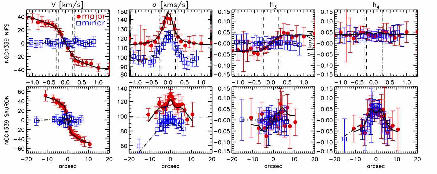
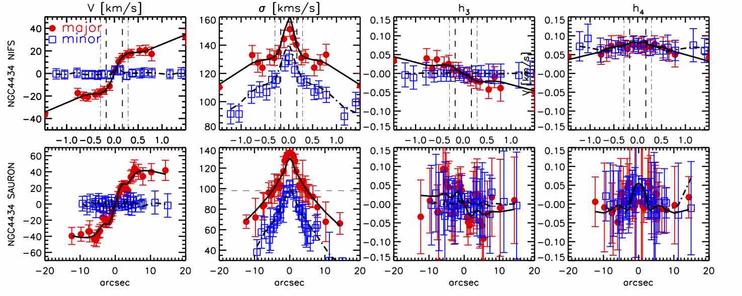
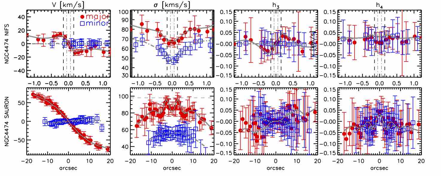
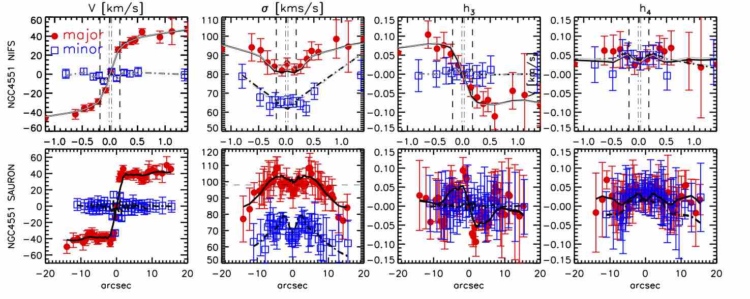
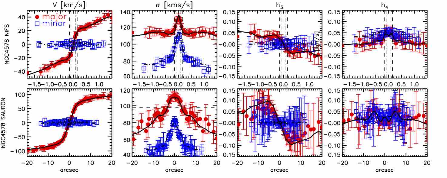
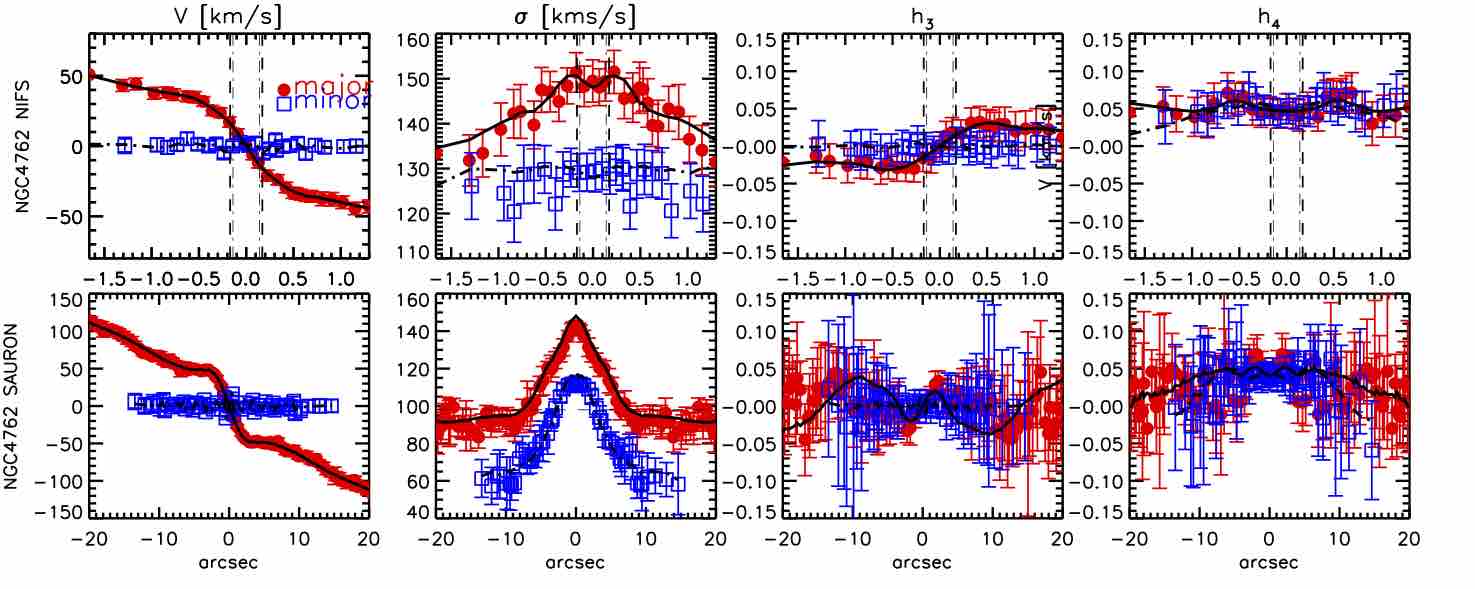
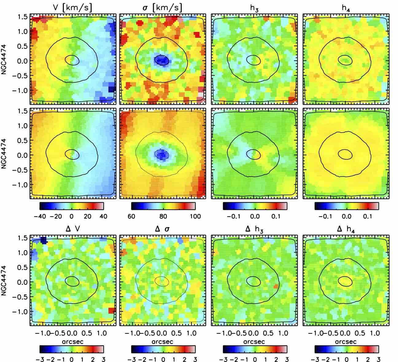
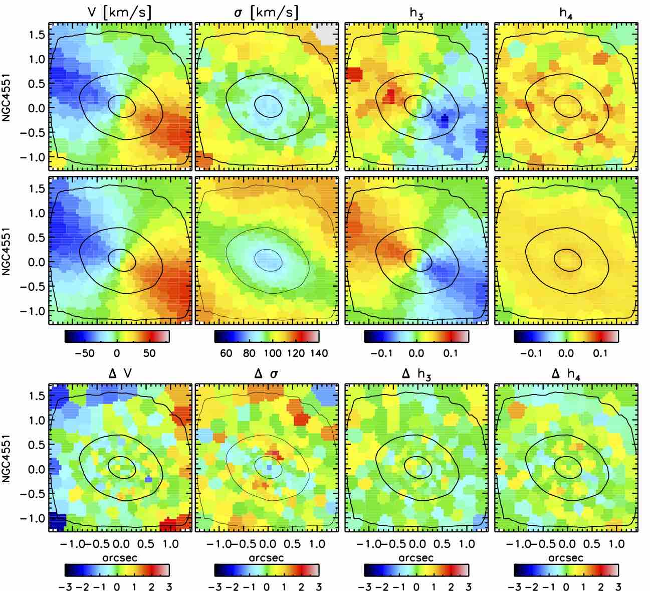
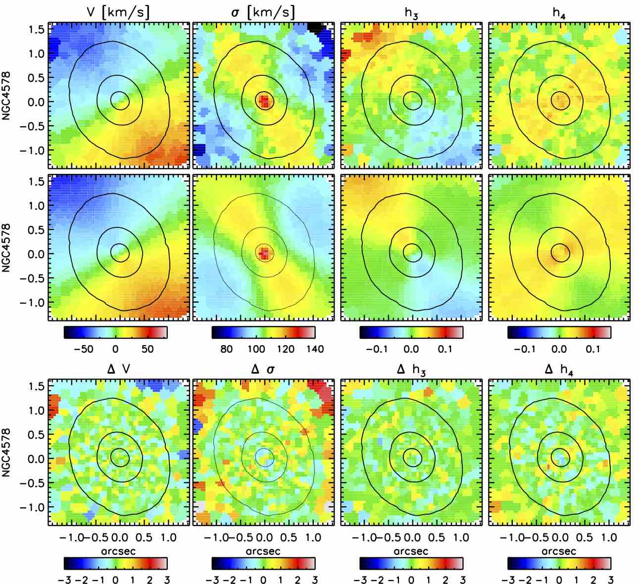
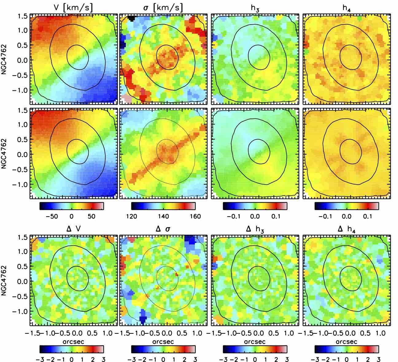
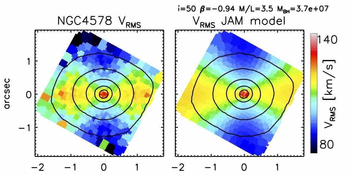
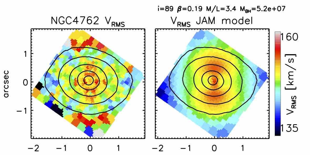
Fig. 2 presents the NIFS kinematics of our sample galaxies, as well as the achieved S/rN across the NIFS field. The lowest S/rN are obtained in NGC 4474, NGC 4339 and NGC 4551. In NGC 4474 the S/rN25 is achieved for bins within the central 1″, while NGC 4339 and NGC 4551 have S/rN30 within the same region, but steeply rising to 40 and 50, respectively. The kinematics follow the properties seen on the SAURON large-scale kinematic maps (see Figs. 18 and 19 and Section 3.2): galaxies show regular rotation, a velocity dispersion peak in the centre, anticorrelated and maps and typically flat and positive maps. The high-resolution data, however, present additional features for two galaxies: NGC 4474 and NGC 4551. In both cases, the velocity dispersion maps show a significant decrease in the centre ( km/s), where the spatial extent of the feature in NGC 4474 is about half the size of the one in NGC 4551 (the galaxies are at similar distances). The structures are within the region of highest S/rN on the maps. For NGC 4474 the typical S/rN is, however, only 30. Nevertheless, at that S/rN, the velocity and velocity dispersion are robustly recovered. We confirmed this by extracting kinematics assuming only a Gaussian LOSVD, as well as extracting kinematics using larger spatial bins and increasing the S/rN. The kinematic components seen in NGC 4474 and NGC 4551 could be associated with dynamically cold structures (e.g. nuclear discs) or could indicate the lack of black holes. Regardless of the origin, they have a profound influence on the determination of the MBH in these galaxies, as will be discussed in Section 5.4. The velocity dispersion maps of NGC 4578 and NGC 4762 are also somewhat unusual, but consistent with the SAURON observations. NGC 4578 shows an elongated structure along the major axis, while the NGC 4762 velocity dispersion map is dominated by an extension along the minor axis.
Aforementioned template mismatch-like features are traced in and maps of NGC4474 and, to a lesser degree, in the map of NGC4551. The maps are not symmetric, as they should be for an even moment of the LOSVD. Similarly, the map of NGC4474 does not show the expected anticorrelation with the velocity map. In order to improve on the high-order moments, we explored a range of pPXF parameters while fitting the spectra, as well as used various combinations of template libraries and extracted the kinematics to an even higher Gauss–Hermite order, but these tests did not improve the fits. In the case of NGC 4474, the most likely reason for the unusual and maps is a combination of the low S/N of the spectra (only about 30), the low inclination, which is likely responsible for the low-level rotation, and therefore an expected low level of anticorrelation between and , and a possible template mismatch. The later is supported also by the test where we forced a high target S/N while binning, which results in a uniform S/rN across the field, and bin sizes of approximately 0.3–0.4″ in diameter. The kinematics extracted from these spectra have the same features as the kinematics presented in Fig. 2: the dip in velocity dispersion, uniform and a non-symmetric . We conclude that the higher order LOSVD moments of NGC 4474 are likely not reliable, which should be kept in mind while interpreting the results, but we use the presented kinematics.
In Fig. 3 we compare the radial profiles of the velocity dispersion and of SAURON and NIFS kinematics. As is evident, the two kinematic data sets are well matched, with some small deviations of the NIFS kinematics. These are noticeable only for the velocity dispersion profiles of NGC4339, which are about 8 per cent lower than those measured with SAURON. In cases of NGC 4434 and NGC 4478 there is a potential offset of less than 5 per cent, but this is within the dispersion of the data points and we do not consider it significant. The NGC 4474 velocity dispersion and compare well with the SAURON data in the overlap region, ensuring at least that the data sets are consistent, if not fully reliable. The influence of the offset for NGC 4339 on the determination of the MBH will be discussed later in Section 4, but our general conclusion is that the two sets of kinematics compare well and can be used as they are.

3.2 SAURON stellar kinematics
Observations, data reduction and the extraction of stellar kinematics for the ATLAS3D Survey is described in detail in Cappellari et al. (2011a), and here we only briefly repeat the important steps of the extraction of stellar kinematics888Available from http://purl.org/atlas3d. The SAURON data were spatially binned using the adaptive Voroni binning method of Cappellari & Copin (2003) using a target S/N of 40. The stellar kinematics were extracted using pPXF (Cappellari & Emsellem, 2004) employing as stellar templates the stars from the MILES library (Sánchez-Blázquez et al., 2006). The SAURON kinematic maps are presented in Figs. 18 and 19. The errors were estimated using a Monte Carlo simulation, and the mean values are given in Table 4 for comparison with the NIFS data.
As discussed in detail in Cappellari & Emsellem (2004), once the galaxy velocity dispersion falls below the instrumental velocity dispersion (), the extraction of the full LOSVD becomes an unconstrained problem. For SAURON data, km/s, and spectra with an intrinsic will essentially not have reliable measurements of the and moments. The pPXF penalizes them towards zero to keep the noise in and under control. At larger radii covered by SAURON FoV, all our galaxies fall within this case, which is visible on the maps of and in Figs. 18 and 19. Even within the central 3″″ this is true for NGC 4474, NGC 4551 and partially for NGC 4578. This problem does not arise for NIFS data as the instrumental resolution is about 30km/s. This means that large-scale SAURON and values for our galaxies are at least partially unconstrained. The comparison of the radial profiles in Fig. 3 suggests that the SAURON data, at least within the central regions, crucial for the recovery of the central black hole mass, are acceptable. Still, as the full LOSVD is necessary to constrain the construction of orbit-based dynamical models employed in this paper, the results of this modelling should be verified in an independent way. This can be achieved with dynamical models that use only the first two moments of LOSVD ( and ), specifically their combination . Therefore we also extracted the mean velocity and the velocity dispersion parameterizing the LOSVD in the pPXF with a Gaussian, for both NIFS and SAURON data. The and extracted in such way are fully consistent with those presented in Figs. 2, 18 and 19. The uncertainties were calculated using the Monte Carlo simulation as before, but with penalization switched off. In this way, even if the LOSVDs are penalized their uncertainties carry the full information on the possible non-Gaussian shapes.
4 Dynamical models
4.1 Methods
The current method of choice for determining MBH is an extension of the Schwarzschild (1979) method, which builds a galaxy by a superposition of representative orbits in a potential of a given symmetry. In axisymmetric models, the orbits are specified by three integrals of motion: energy , the component of the angular momentum vector along the symmetry axis , and the analytically unspecified third integral . This method was further developed by a number of groups to be applied on axisymmetric galaxies when both photometric (the distribution of mass) and kinematics (the LOSVD) constraints are used (Richstone & Tremaine, 1988; Rix et al., 1997; van der Marel et al., 1998; Cretton et al., 1999; Gebhardt et al., 2003; Valluri et al., 2004; Thomas et al., 2004), using IFU data (Verolme et al., 2002; Cappellari et al., 2006), as well as extended to a more general triaxial geometry (van den Bosch et al., 2008).
Both the strengths and the weaknesses of the Schwarzschild method lie in its generality. Earlier papers pointed out possible issues with black hole mass determinations (Valluri et al., 2004; Cretton & Emsellem, 2004), but detailed stellar dynamical models of the two benchmark galaxies with the most reliable independent MBH estimates NGC4258 (Siopis et al., 2009; Drehmer et al., 2015) and the Milky Way (Feldmeier et al., 2014; Feldmeier-Krause et al., 2017), using both anisotropic Jeans (Cappellari, 2008) and Schwarzschild’s models, demonstrated that, in practice, both methods can recover consistent and reliable masses. The main source of error are systematics in the determination of the stellar mass distribution within the black hole SoI, which is generally not included in the error budget.
The extent of the kinematic data used to constrain Schwarzschild models is also of high importance (Krajnović et al., 2005). Outside the regions covered by, for example, a few long slits, the Schwarzschild method, due to its generality, is a poor predictor of stellar kinematics (Cappellari & McDermid, 2005). The IFUs have helped decrease this problem, but to robustly recover MBH one still needs to cover at least the area within a half-light radius of the galaxy (Krajnović et al., 2005), but also map the stellar LOSVDs in the vicinity of the black hole (Krajnović et al., 2009). It is also important to allow for sufficient freedom in the models, for the shape of the total mass density to properly describe the true one, within the region where kinematics is fitted. This implies that, if one includes in the models kinematics at large radii (i.e. Re), where dark matter is expected to significantly affect the mass profile, one should explicitly model its contribution, to avoid possible biases in the black hole masses (Gebhardt & Thomas, 2009; Schulze & Gebhardt, 2011; Rusli et al., 2013). Finally, the recovery of the intrinsic shape of the galaxy is only possible for specific cases (van den Bosch & van de Ven, 2009), as the Schwarzschild method, even when constrained by large-scale IFU data, suffers from the degeneracy in recovery of the inclination (Krajnović et al., 2005). As shown by van den Bosch & van de Ven (2009), while it is possible to determine whether the potential has an axial or triaxial symmetry, only the lower limit to the inclination of an axisymmetric potential imposed by photometry is constrained (one should also keep in mind the mathematical non-uniqueness of the photometric deprojection, e.g. Rybicki, 1987). Similarly, the viewing angles of a triaxial system can be determined only if there are strong features in the kinematic maps such as kinematically distinct cores.

An alternative, less general but consequently less degenerate, is to solve the Jeans equations. The standard approach consists of assuming a distribution function which depends only on the two classic integrals of motion (, ) (Jeans, 1922). In this case the velocity ellipsoid is semi-isotropic: and , where and are the velocity dispersions along the cylindrical coordinates and (e.g. Magorrian et al., 1998). Allowing for the anisotropy of the velocity ellipsoid introduces two additional unknowns: the orientation and the shape of the velocity ellipsoid. One approach to introduce the anisotropy is based on an empirical finding that the velocity ellipsoid is flattened in the -direction (the symmetry axis) and to first order oriented along the cylindrical coordinates (Cappellari et al., 2007)999Cappellari et al. (2007) work was based on Schwarzschild models of 24 galaxies. JAM models were in the mean time successfully applied on the 260 galaxies of the ATLAS3D Survey confirming that the assumptions built in the JAM models are adequate for ETGs.. Jeans anisotropic modelling (JAM; Cappellari, 2008) follows an approach where the velocity anisotropy is introduced as , defining the shape of the velocity ellipsoid, oriented along the cylindrical coordinates. Characterizing the surface brightness in detail leaves four unknowns that have to be constrained by the IFU kinematics: mass-to-light ratio (), inclination , anisotropy , and, if the data support it, mass of the black hole, MBH. This assumption on the velocity ellipsoid, while not exactly valid away from the equatorial plane or far from the minor axis, seems to work remarkably well on real galaxies (Cappellari et al., 2013a), even allowing for a determination of the inclination (Cappellari, 2008), at least for fast rotators (see for a review section 3.4 of Cappellari, 2016), as well as oblate galaxies in numerical simulations (Lablanche et al., 2012; Li et al., 2016). Recently, a major comparison between Schwarzschild and JAM modelling (Leung et al., 2018), for a sample of 54 S0–Sd galaxies with integral-field kinematics from the EDGE-CALIFA survey (Bolatto et al., 2017), found that the two methods recover fully consistent mass density profiles.
A further difference between the orbit and Jeans equation-based modelling is that the latter is constructed such that it is constrained by the second velocity moment only, without the need for the higher parametrization of the LOSVD. The second velocity moment can be approximated by the combination of the observed mean velocity and the velocity dispersion, (Cappellari, 2008), simplifying the requirements on the data quality. For these reasons, we will use both modelling approaches in determining MBH of our targets. We will fit the NIFS data only with JAM models and then both the NIFS and SAURON data with Schwarzschild models.
We note that in a number of other studies where the two methods were compared in detail (Cappellari et al., 2010; Seth et al., 2014; Drehmer et al., 2015; Feldmeier-Krause et al., 2017; Thater et al., 2017), black hole masses from JAM and Schwarzschild modelling were found to agree well. NGC4258 and the Milky Way deserve a special attention as their MBH are the most secure and based on methods different from those discussed here. In the case of NGC 4258, the Siopis et al. (2009) result is within 15 per cent of the maser MBH, while the Drehmer et al. (2015) result is within about 25 per cent. The difference between Siopis et al. and Drehmer et al. black hole masses are consistent at level. In the case of the Milky Way, Feldmeier-Krause et al. (2017) modelled the black hole with both Schwarzschild and JAM methods and presented results that are consistent within level.
These results are fully consistent with tests between Schwarzschild methods based on the same data. Such studies are regrettably rare, but the most recent were done for two galaxies: M32 (Verolme et al., 2002; van den Bosch & de Zeeuw, 2010) and NGC 3379 (Shapiro et al., 2006; van den Bosch & de Zeeuw, 2010). In the case of M32 the results are consistent at confidence level, while MBH estimates for NGC 3379 are within confidence level, but differ for more than a factor of 2.
In this work, we also add NGC 1277, for which we show in Appendix A that JAM can provide results consistent with the Schwazschild models. This last example demonstrates the usefulness of applying independent approaches to the same data, as we do here, to increase the confidence in our results. Both methods can potentially produce results of limited fidelity. In case of the more general Schwarzschild models the numerical noise, as well as the issues discussed above, can limit the quality of the data, as much as the lack of generality and possible degeneracies (i.e. mass – anisotropy, but see Gerssen et al., 1997) are limiting JAM models. The agreement between these different methods provides a certain level of security in the robustness of the results. A disagreement in the modelling results, however, would be inconclusive as to which solution is more trustworthy beyond the statement that JAM models lack generality.
Note that we do not include dark matter in any of our models, and we postpone the discussion on possible consequences to Sections 4.3 and 5.1.

4.2 Mass models
The first step in the construction of dynamical models is a detailed parametrization of the surface brightness distribution. Our approach is to use the MGE method (Emsellem et al., 1994) and the fitting method and software of Cappellari (2002, see footnote 7 for the software). We used both the HST imaging and SDSS data, as they were presented in Scott et al. (2013a). The SDSS images were in the band while the HST images were obtained with two instruments (WFPC2 and ACS), and we selected those filters that provided the closest match to the SDSS images (see Table 2). We fitted the MGE to both images simultaneously, fixing the centres, ellipticities and the position angles of the Gaussian components, and scaling the outer SDSS light profiles to the inner HST profiles by ensuring that the outer parts of the HST profiles smoothly join with the SDSS data. In this way the HST images provide the reference for the photometric calibration.
When moving to physical units, we followed the WFPC2 Photometry Cookbook101010http://www.stsci.edu/hst/wfpc2/analysis/wfpc2cookbook.html and converted from the STMAG to Johnson R band (Vega mag), assuming MR=4.41 for the absolute magnitude of the Sun (Blanton & Roweis, 2007), and a colour term of 0.69 mag (for a K0V stellar type). For ACS images we followed the standard conversion to AB magnitude system using the zero-points from Sirianni et al. (2005) and assuming a M5.22 mag for the absolute magnitude of the Sun111111http://www.ucolick.org/cnaw/sun.html. For all galaxies we accounted for the galactic extinction (Schlafly & Finkbeiner, 2011). We list the parameters of the MGE models in Table 7 and in Fig. 4 we show the comparison between the MGE models and the HST data.
Fig. 4 shows that MGE models reproduce well the central regions of our galaxies, except partially the disc in NGC 4762, where the largest deviations are less than 10 per cent. Reproducing this transition between the bulge and the disc along the major axis would require negative Gaussians. As these are not accepted by our modelling techniques, we do not attempt to improve the fit in this way. As we show later in the dynamical models this does not have an impact on the results. Overall, the surface brightness distributions of our galaxies are consistent with axisymmetry, showing no evidence of changes in the photometric or kinematic position angles with radius).
4.3 JAMs
As our galaxies are part of the ATLAS3D sample, they were already modelled with JAM in Cappellari et al. (2013a). These models were constrained by the SAURON kinematics only and used SDSS images for parametrization of light. The models also included various parametrization of the dark matter haloes. Alternative JAM models of ATLAS3D galaxies, with no direct parametrization of the dark matter, but instead fitting for the total mass, were also presented in Poci et al. (2017). These previous works explored global parameters of our galaxies, including the dark matter fraction and the inclination, assuming axisymmetry. We build slightly different JAM models, constrained with only the NIFS kinematics, and MGE models fitted to the combined HST and SDSS imaging data (see Section 4.2). We assume the inclination given by models from Cappellari et al. (2013a), listed in Table 2. To constrain the JAM models we use the second velocity moment, as described in Section 3.2. Unlike for the Schwarzschild models, in the case of the JAM models, there is no need for large scale kinematics to constrain the fraction of stars on radial orbits. This is because the kinematics of the whole model is already uniquely defined by the adopted model parameters. For this reason, the best estimates of black hole masses are obtained when fitting the kinematics over the smallest field that is sufficient to uniquely constrain the anisotropy, MBH and (e.g. Drehmer et al., 2015). In this way one minimizes the possible biases in the JAM models caused by spatial variations in anisotropy or in the galaxy, without the need to actually allow for these parameters to vary in the models.
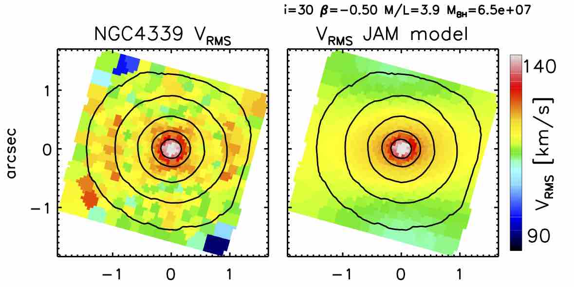
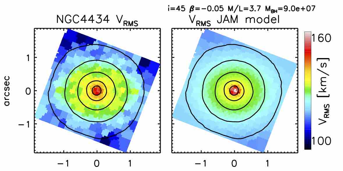
The JAM models based on SAURON data constrain the inclination of two galaxies to be edge-on (close to 90∘), but most galaxies have a low inclination. As models on low inclinations are more degenerate, to explore the parameter space we also run models assuming an edge-on orientation (in practice, ∘) for these galaxies. Therefore, each JAM model assumes an axisymmetric light distribution at a given inclination, and has additional three free parameters. Two of those are used to fully specify the distribution of the second velocity moment (at a given inclination): a black hole mass M and a constant velocity anisotropy parameter . The ratio is then used to linearly scale the predicted second velocity moment to the observed Vrms. We build a grid of models varying M and . These are shown in Fig 5 and the best-fitting parameters are presented in Table 5.
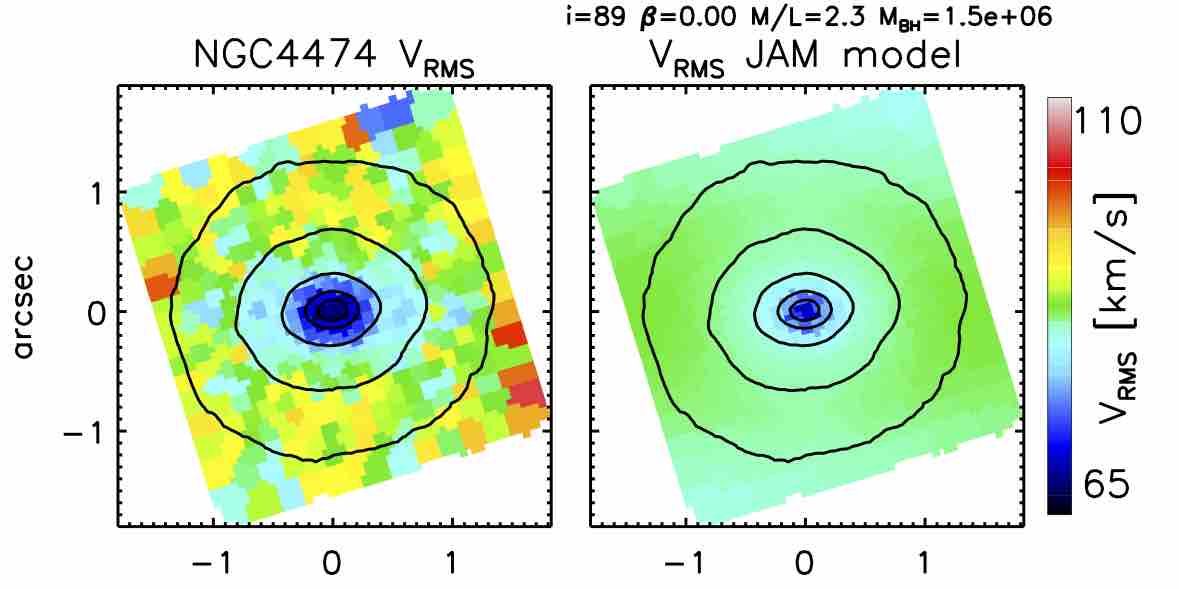
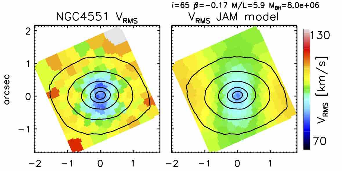
NIFS data have a small angular coverage, but in the majority of cases they are able to constrain the black hole and the velocity anisotropy. The JAM models provide only an upper limit at the confidence level for black hole masses in NGC 4474 and NGC 4551, although in the latter case there is also a lower limit at confidence level, suggesting a low-mass black hole of M⊙. The velocity anisotropy is poorly constrained for NGC 4339 and NGC 4578, also being unusually low for ETGs. These values are however unreliable as the galaxies are oriented at low inclinations (∘) and cannot be trusted (Lablanche et al., 2012). In cases where the anisotropy can be trusted, galaxies are either isotropic (NGC 4474) or mildly anisotropic with negative (NGC 4551) and positive (NGC 4762) .


Changing the inclination of the models does not change the results substantially, and the largest difference is seen at the lowest inclination. NGC 4339 is nominally at only 30∘ and putting the models at 89∘ changes the shape of the contours significantly. At 89∘ the best-fitting model is almost isotropic, but the M does not change. A similar effect is seen for NGC 4578 (∘). The change of inclination has a minor effect on the estimated .
As our galaxies are at different distances the NIFS data probe different physical radii in their nuclei. Based on the JAM models, the SoI sizes of the best-fitting black holes span a range from 0.1 to 0.4″. This means that the dynamical models are constrained by kinematics which covers from about 4 to about 14 times the radius of the SoI. In order to verify that we are indeed probing a sufficient areas to constrain the anisotropy, MBH and , we performed the following test. The NIFS data with the largest coverage are for NGC 4578 and NGC 4762 (8 and 14 times the obtained radius of the SoI), while the smallest coverage is found for NGC 4339 and NGC 4434 (4 times the radius of the SoI). Therefore, we run two grids of JAM models for NGC 4578 and NGC 4762 restricting the NIFS field to 4 times their respective radii of SoIs. The resulting grids resemble those in Fig. 5 in terms of the shape of the contours, and also recover similar best-fitting results. In case of NGC 4578, the best fit is given by the same model as in the case of the full field coverage, except that its vertical ansiotropy is less tangentially biased (by 15 per cent). The NGC 4762 best-fitting model has 8 per cent smaller MBH and about 30 per cent smaller anisotropy values, which fall within the uncertainty level of the grid shown in Fig. 5. From these tests we conclude that our NIFS data are adequate to constrain JAM models of all galaxies in the sample.
Mitzkus et al. (2017) constrain their JAM models by propagating uncertainties different from those obtained by extraction of kinematics. Specifically, they assume a constant error on the velocity (5 km/s) and as the uncertainty on the velocity dispersion take 5 per cent its value for each bin. The reason for this is to prevent a biasing of the solution towards the high S/N central pixels. We also run JAM models in such a configuration and recovered the same results. The reason is a relatively small variation of both velocity and velocity dispersion uncertainties across the FoV, as well as the fact that the average uncertainties are actually similar to those proposed by Mitzkus et al. (2017), as can be seen from Table 4.
In Fig. 6, we compare the second velocity moment maps (parameterized as Vrms) and the JAM model predictions for the best-fitting models. We compare the JAM models with bi-symmetrized data (see Section 4.4 for details on how we symmetrize maps), as models have such symmetry by construction. A similar comparison is given also in Fig. 7, this time along the major and minor axes, showing also the error on the Vrms. For NGC 4474 and NGC 4551 we present models with black hole masses corresponding to derived upper limits. All models reproduce the features on the observed Vrms maps reasonably well, while the model maps for NGC 4551 and NGC 4762 are somewhat different from data, systematically under- or overpredicting second velocity moments. These difference, however, are typically within the uncertainties, as seen of Fig. 7. Models for NGC 4474 and NGC 4551 have some difficulties reproducing the extent and the shape of the central decreases in the Vrms, but they are, except when reproducing the minor axis of NGC 4551 generally consistent with the uncertainties. We will further discuss the implications of JAM fits to these two galaxies in Section 5.4.

4.4 Schwarzschild models
We used the ‘Leiden’ version of the axisymmetric Schwarzschild code, as it is described in Cappellari et al. (2006). Briefly, the code takes the MGE parametrization of light and, assuming an inclination, an ratio, and axisymmetry, deprojects the surface brightness distribution into a mass volume density, which, after addition of a black hole of a certain mass (MBH) specifies the potential. The next step is generation of a representative orbit library for a given set of and MBH. Each orbit is specified by three integrals of motion (, , ). We sample with 21 logarithmically spaced points giving the representative radius of the orbit, and at each energy we use eight radial and seven angular points for sampling and respectively. As orbits can have a prograde and retrograde sense of rotation, the initial set of orbits is doubled and there are 2058 orbital bundles. Each bundle is composed of individual orbits started from adjacent initial conditions. In total, there are orbits which make the basis for the construction of the galaxy. The phase space coordinates are computed at equal time steps and projected on the sky plane as triplets of coordinates (, , ), while the sky coordinates (, ) are randomly perturbed with probability described by the PSF of the data. The model galaxy is Voronoi binned in the same way as the observed kinematics and at each bin position the code fits the resulting LOSVDs to provide , and four Gauss-Hermite parameters (up to ). As the dithering scheme improves on the smoothness of the distribution function, we use only a modest amount of regularization (as defined in van der Marel et al., 1998), except for NGC 4762 for which we increased it to in order to make the resulting orbital weights distribution smoother, which also reflected in somewhat smoother contours on the model grids (see below)121212We have nevertheless run models at both and 10 regularizations and in all cases, including the NGC 4762, the results were fully consistent..

For each galaxy we run a grid of models specified by and MBH. Given the inclination degeneracy (Krajnović et al., 2005), we do not try to fit for the galaxy inclination, but adopt the values given in Table 1. A new orbital library is produced for each MBH at the best-fit inferred from the JAM models (Section 4.3), and scaled to a range of ratios. The initial choice for MBH was the one predicted by the M relation. The models are constrained with NIFS and SAURON kinematics fitted simultaneously. As the models are by construction bi-(anti-)symmetric, with the minor axis of the galaxy serving as the symmetry axis, we symmetrize the kinematics in the same way. This was done by averaging the kinematics of the positions ((,), (, ), (,), (,)). Given that the data are Voronoi binned and that the bins at the four positions are not necessarily of the same shape and size, when there are no exact symmetric points, we interpolated the values on those positions and then averaged them. When averaging we take into account that the odd moments of the LOSVD ( and ) are bi-anti-symmetric, while the even moments (, ) are bi-symmetric. We retain the original kinematic errors at each point, however, so as not to underestimate the LOSVD parameter errors and over-constrain the model with artificially low formal errors. During the fitting process we model the full extent of the data and used them to derive the overall sum (note that even though we symmetrize the data, we do not fold it or fit only one quadrant). Finally, we exclude the central 1.3″ of the SAURON data since these overlap with the high resolution NIFS observations, and we wish to avoid our results being affected by inconsistencies in the relative calibration or assumed PSFs of the two data sets. In practice, however, fitting both data sets in the overlap region does not make a significant difference, as also reported earlier (Krajnović et al., 2009; Thater et al., 2017).
Notes – Column 1: galaxy name; Column 2-6: parameters of the JAM models (black hole mass, mass-to-light ratio, velocity anisotropy, of the best fit model per degree of freedom (DOF)); Columns 6 - 8: parameters of the Schwarzschild models (black hole mass, mass-to-light ratio, and of the best fit model per DOF ). Uncertainties were estimated by marginalising over the other parameter (MBH, or M/L) and assuming a confidence level for one degree of freedom. Note that JAM models were constrained using original kinematics, while Schwarzschild models were constrained using symmetrised kinematics. M/L are given in Johnson -band magnitude system for WFC2 galaxies (NGC 4339, NGC 4474 and NGC 4578) and for F450W-band of the AB magnitude systems for galaxies observed with ACS (NGC 4434, NGC 4551 and NGC 4762).
Figure 8 shows the model grids for all galaxies in the sample. We measure MBH at the confidence level for four of the six objects, with the remainder giving only upper limits. The results are again outlined in Table 5, where one can see that the results from the JAM modelling are fully consistent with the Schwarzschild results within level or better. The parameter uncertainties from the Schwarzschild modelling were estimated by marginalizing along the best-fitting ratio and MBH and for the confidence level (for one degree of freedom). We choose the level because levels often do not have a single well defined minimum, due to numerical discretization noise. In all cases is well constrained, and the contours are regular and show only a minor degeneracy between M/L and MBH (e.g. NGC 4339). For NGC 4762, there were multiple local minima apparent even at the confidence level. Increasing the level of regularization from to avoided this issue, but there is still evidence for degeneracy towards higher black hole masses. As shown below, this is not significant and the mass of the black hole is well constrained. For NGC 4474 and NGC 4551, the contours do not close over 2-3 order of magnitude in MBH (down to a few times M⊙). In both cases, there are tentative level lower limits for best-fitting black holes of and M⊙, respectively, but these should not be considered reliable, as discussed below.
Our results can be compared to those of (Cappellari et al., 2013a) who modelled the full ATLAS3D sample, in particular with their ratios. They work in SDSS band and we need to first adjust for the difference in the filter and the photometric systems. Using the web tool based on Worthey (1994) models131313http://astro.wsu.edu/dial/dial_a_model.html, we estimate that to change from our Johnson R and F450W AB systems to SDSS AB system we need to apply factors of 1.25 and 0.85, respectively. This means that our based on the Schwarzschild models (and approximately within one effective radius) are 5.0, 2.8, 3.0, 4.6, 4.6 and 3.1 for NGC 4339, NG 4434, NGC 4474, NGC 4551, NGC 4578 and NGC 4762, respectively. A comparison with the values published in (Cappellari et al., 2013a) shows that the differences between respective are small, typically below 10 per cent, except for NGC4762 where they are about 17 per cent.
This comparison, as well as girds on Fig. 8, show that the results of Schwarzschild models compare well with the results of the JAM models within a uncertainty level. This is both encouraging and revealing, as our approach is purely empirical. In this paper we use two different methods (one more general, but containing possible numerical issues, and another less general, but numerically accurate) to measure the same quantity. This is motivated by the agreement found for a number of other black hole mass estimates, as outlined in Section 4.1, including the most precisely known black holes in the Milky Way and the megamaser galaxy NGC 4258, as well as in the somewhat controversial case of NGC 1277 (which we show in Appendix A). The fact that such different modelling techniques, with their inherent assumptions and sources of systematics, as well as constrained by different data sets (NIFS only for JAM and SAURON and NIFS for Schwarzschild), give consistent results, allows us to trust the derived MBH. On the other hand, a disagreement between JAM and Schwarzschild results would have to be taken with a caution. The lack of generality of JAM models could be the source of such a disagreement (for potential issues with Jeans models in spherically symmetric case see Mazzalay et al., 2016), but numerical inaccuracies of the Schwarzschild model could also bias the results (e.g. appendix A in Zhu et al., 2018). The fact that they are, in our case, consistent typically at level (except for one galaxy where the difference is just above level), and are consistent with previous comparisons between black hole mass estimates (e.g. Siopis et al., 2009; van den Bosch & de Zeeuw, 2010; Walsh et al., 2013; Drehmer et al., 2015; Feldmeier-Krause et al., 2017; Davis et al., 2017), discloses how much one can trust black hole mass measurements in general, which should also be considered when discussing the black hole mass scaling relations.
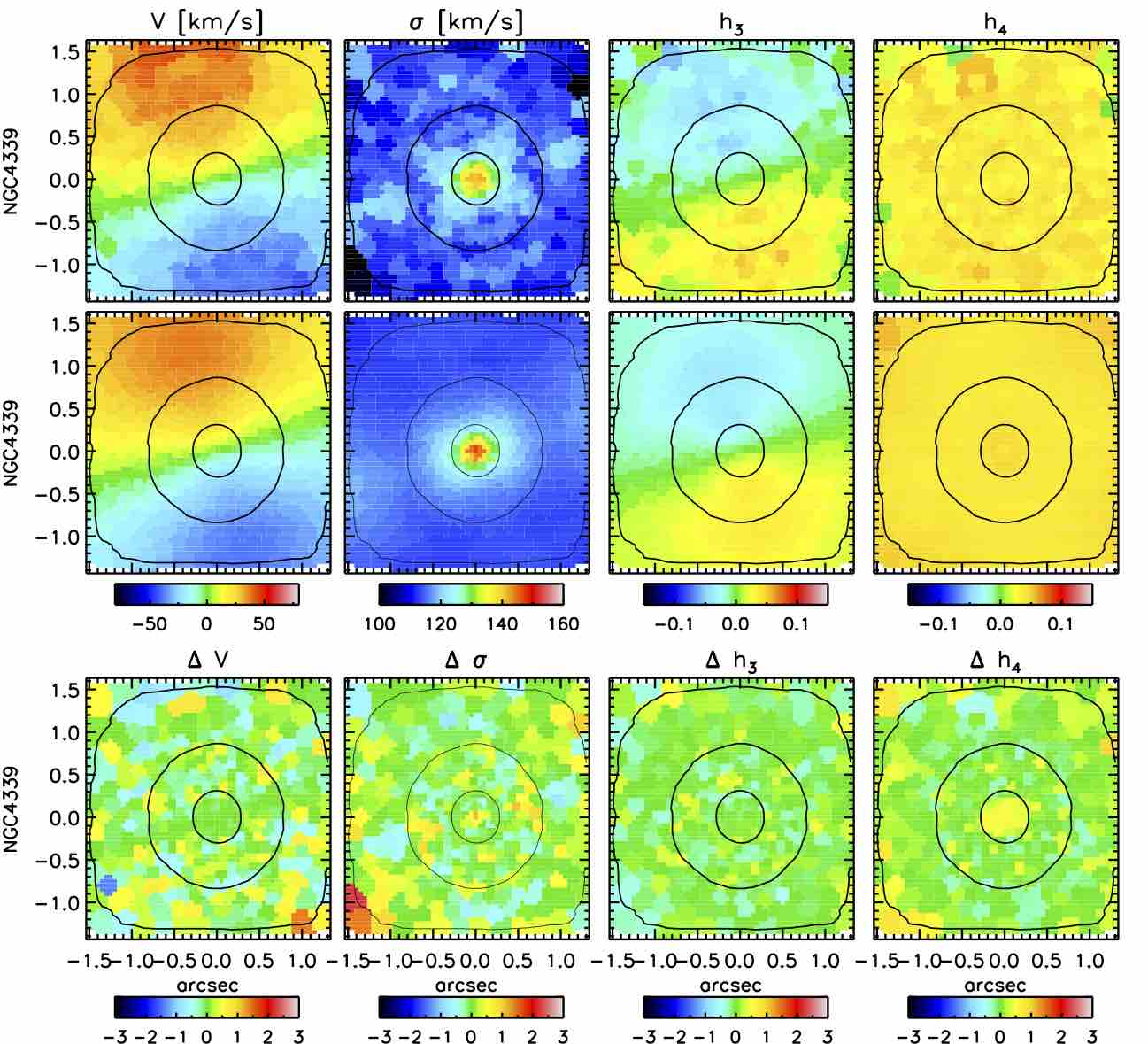
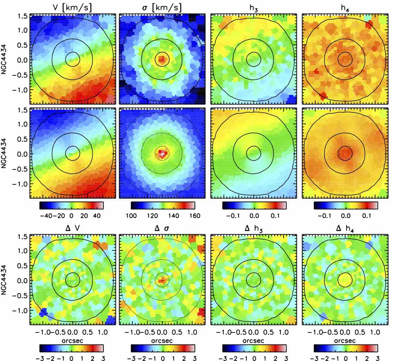
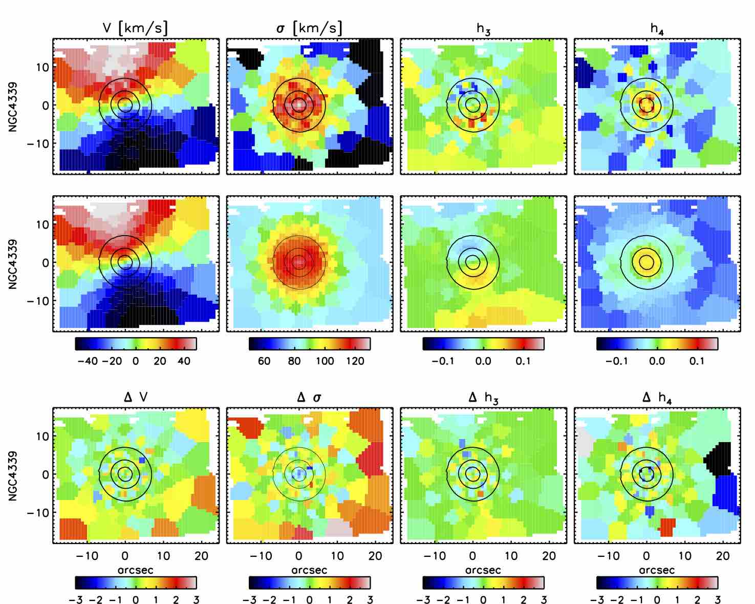
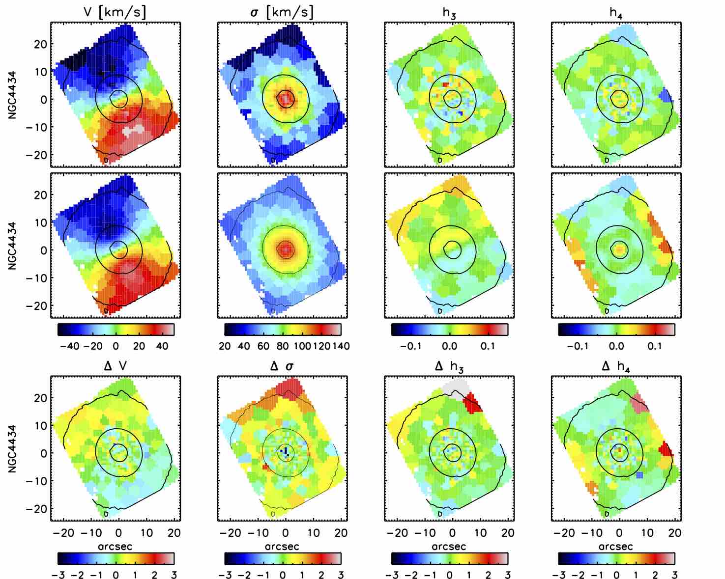
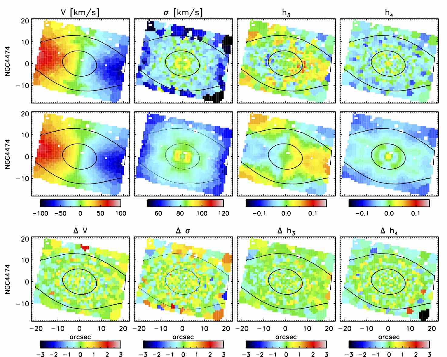
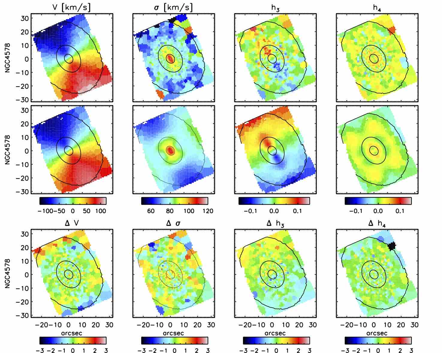
The (symmetrized) data – model comparison for all galaxies are shown in Figs. 22 and 23, indicating that our best-fitting models can reproduce all features rather well, both on the high-resolution NIFS data and the large-scale SAURON data. The quality of fits are best seen in the residual maps, which show the difference between the model and the data relative to the uncertainty for a given kinematic map. Typical disagreement between the best-fitting models and the data are within the uncertainties ( level), with some level discrepancies for individual bins (often towards the edge of the field). Even NGC 4474 and NGC 4551 models (at the formally best-fitting MBH) reproduce well the full extent of the NIFS and SAURON kinematics.
In Fig. 9 we compare the velocity dispersion maps between the data and the models for the best fit, a lower and a higher mass MBH (just outside the contours). The differences between the models are obvious, clearly indicating that the data provide robust upper and lower limits on the masses of black holes. As expected, this is not the case for NGC 4474 and NGC 4551, for which the models with the lowest probed MBH show essentially the same kinematics as the observed data. To emphasize this we selected models which are outside of the level contours on the lower side of the formally best-fitting model. The differences between these maps and the data are essentially negligible. On the other hand, comparing the data with a model outside of the level contour (the upper limit), shows the difference in the central velocity dispersion. This means that one should take the results with caution, and we consider only the level as a robust estimate on the uncertainty of the Schwarzschild models. In case of NGC 4474 and NGC 4551, this means we can trust only the upper limits. Similarly, the robustness of the estimated uncertainties for NGC 4762 can be seen in comparison of the data with a model with MBH just above the limit. This model is located within the plateau in Fig. 8, its MBH creates a marginally different velocity dispersion map from the best fitting model, indicating the level at which the upper limit of MBH can be trusted.
5 Discussion
5.1 Possible systematics and their influence on the results of dynamical models
The velocity dispersions discrepancy for NGC 4339. As shown in Fig. 3, there is a minor difference in the measured velocity dispersions using the NIFS and SAURON data of NGC 4339. In the overlap region between the two data sets, the NIFS velocity dispersion are lower for about 8 per cent. We run the Schwarzschild models using these data. As for all galaxies we excluded the SAURON data in the overlap regions. In order to test the robustness of these result we also run additional models which had the following modifications: (i) both NIFS and the central SAURON data were included, and (ii) we corrected the NIFS data by increasing the velocity dispersions by 8 per cent. Both of these models gave fully consistent results with the base models. The ratio did not change. This was expected as is mostly constrained by the large-scale SAURON data. The mass of the black hole did show a minor change. In the case (i) it increased for 7 per cent to and in the case (ii) for about 80 per cent to . Both of these values are within the confidence contours and indicate the possible range of MBH due to systematics in the data.
Possible influence of the dark matter. Cappellari et al. (2013b) and Poci et al. (2017) evaluated the dark matter content of our galaxies based on the SAURON kinematics. This was done through JAM dynamical models which had fitted only a total mass profile or a combination of the stellar and dark matter profiles. The results are generally consistent, and, specifically, for our galaxies provided the following fractions of dark matter within one half-radii: (Cappellari et al., 2013b) and for (using Model I in Poci et al., 2017) for NGC 4339, NGC 4434, NGC 4474, NGC 4551, NGC 4578 and NGC 4762, respectively. It is evident that most of galaxies have a negligible contribution of DM in the regions covered with our kinematics. NCG 4578 and NGC 4762 are somewhat different with possibly significant contribution of dark matter. In Section 4.4 we showed that our derived via Schwarzschild modelling are comparable with the JAM ratios of paper Cappellari et al. (2013a), therefore we can relate our results directly to the work of the two studies above. Comparing our M/L ratios with those of stellar populations published in (Cappellari et al., 2013b) and adjusted for the filter band difference, stellar population based on the Salpeter (1955) initial mass functions (IMF) are larger than dynamical values we estimate. Therefore, a Kroupa (2002) or a Chabrier (2003) IMF based would be more physical, as expected given the trends between the IMF and the stellar velocity dispersion or mass of the galaxies (e.g. van Dokkum & Conroy, 2010; Thomas et al., 2011; Conroy & van Dokkum, 2012; Cappellari et al., 2012; McDermid et al., 2014; Spiniello et al., 2014).
Our JAM (Section 4.3) and Schwarzschild models (Section 4.4) are based on data that probe very different scales. The JAM models, based only on NIFS data, probe only a few per cent of the half-light regions in our galaxies, while Schwarzschild models take the full extent of the SAURON data into account, which except for NGC 4762 map the full half-light region of the sample galaxies. In all cases, and specifically for galaxies with possible significant fraction of dark matter, the models give very consistent results (Tabel 5), in terms of the (less than 10 per cent difference), MBH (within a factor of 2), and the orbital anisotropy (the latter point will be discussed in Section 5.3). Specifically, the similarity of is rather surprising as they are constrained by very different radii. Both types of models, however, are able to reproduce the main features visible in the kinematics data, and by giving consistent solutions for the free parameters they raise the confidence in the results. For this reason, we do not explore further the influence of the dark matter on the dynamical models.
Variations in stellar populations. McDermid et al. (2015) presented the star formation histories of ATLAS3D galaxies and from these data one can derive the radial variation of the stellar population parameters and their mass-to-light ratio . For our galaxies there is a mild radial decrease in of up to 30 per cent across the region covered by SAURON data (Poci et al., 2017)141414Maps of ratios for ATLAS3D galaxies are available on the project website: http://purl.org/atlas3d. Our models do not take into account a variable M/L (see Section 5.4), but we do not find a significant difference in derived from small scale JAM and full scale Schwarzschild models. The grids of Schwarzschild models show no or only a weak dependance between the M/L and MBH (see contours in Fig. 8), the strongest of which is for NGC 4339. We therefore assume that the impact of the variable is minor to the final results of this work
5.2 Additions to the scaling relations
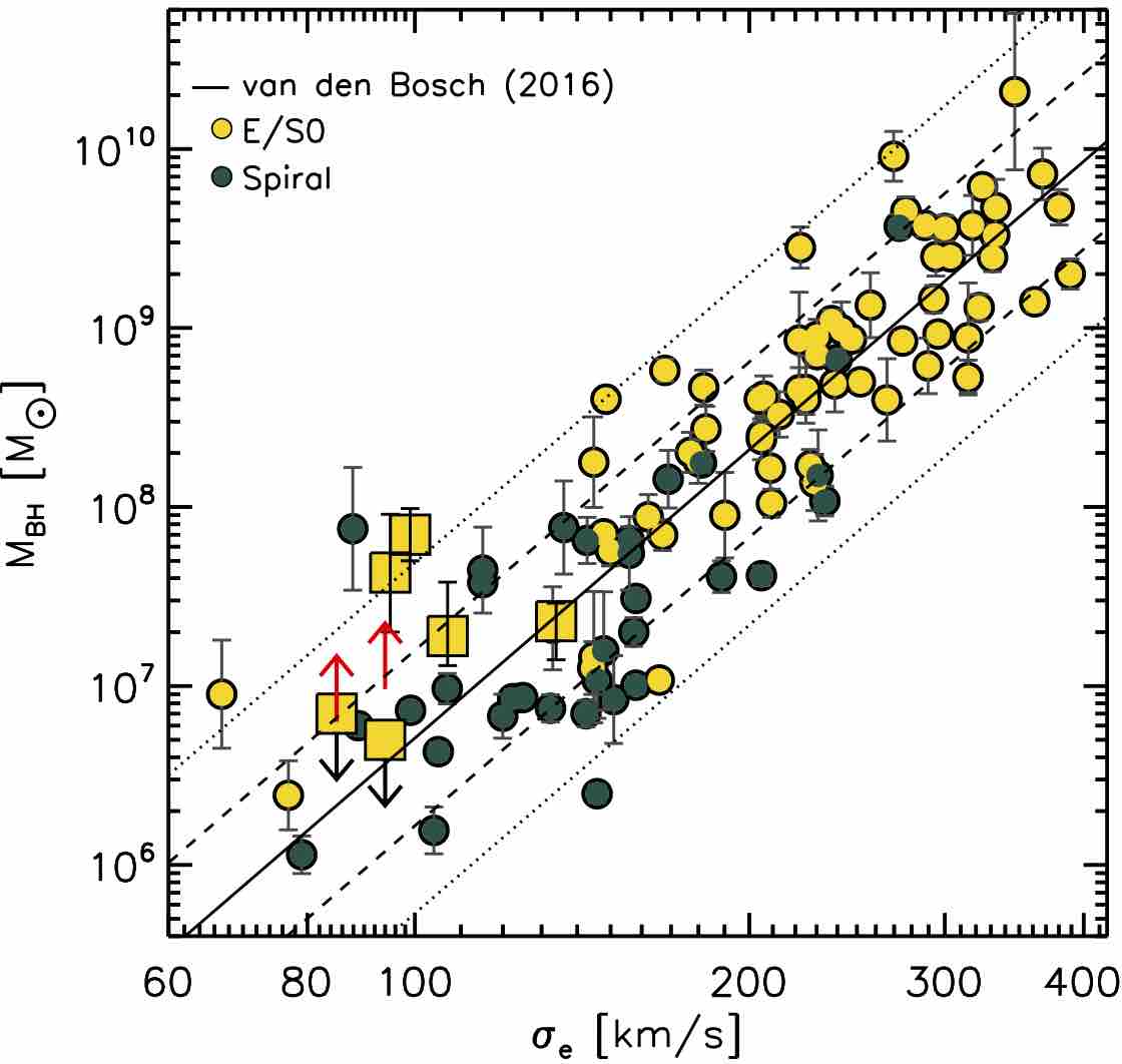
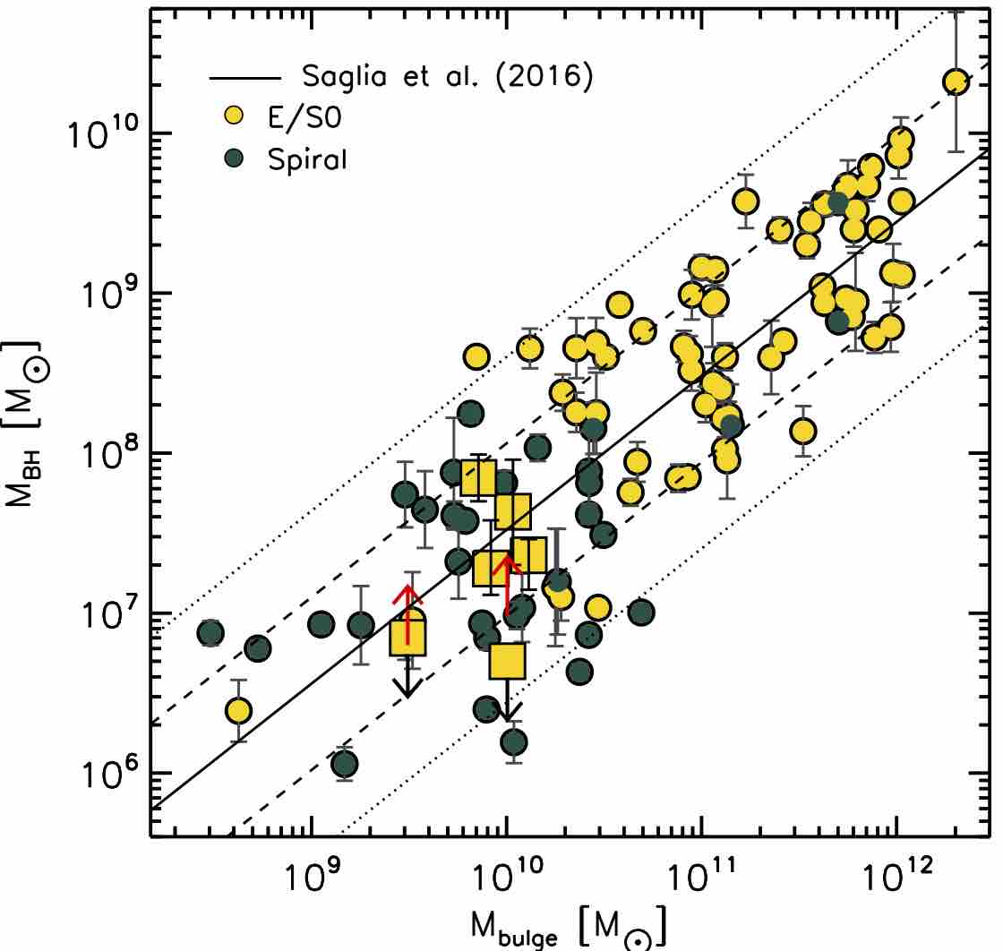
We place our galaxies on the M and MMbulge (bulge mass) relations based on a recent compilation of black hole measurements (Saglia et al., 2016) in Fig. 10. Looking at the M relation, there are two galaxies (NGC 4339 and NGC 4434) that are significantly above the relation (about away), while two (NGC 4578, and NGC 4762) lie on the relation. The two upper limits place the galaxies above the relation. Assuming that we could measure a black hole mass that has an SoI 3 times smaller than the resolution of the LGS kinematics, we could just detect black holes in those galaxies with masses within the scatter of the M scaling relation.
The situation is somewhat different on the MMbulge relation as all detections are now within the scatter of the relation, while the galaxies with the upper limits fall below the relation. We note that the position of our galaxies on this diagram is critically dependent on the estimates of the bulge mass. We use values from Table 1, derived from the total galaxy mass (Cappellari et al., 2013b) and the disc–bulge decomposition of Krajnović et al. (2013a).
Kinematically our galaxies are all fast rotators, with regular, disc-like rotations. Morphologically, they seem to consist of a spheroid and an outer disc, which are easily recognizable only in the two galaxies seen at an inclination near 90∘(NGC 4474 and NGC 4762). Ferrarese et al. (2006) fit the HST/ACS surface brightness profiles of five of our galaxies (all except NGC 4339) with Sersic (Sérsic, 1968) and core-Sérsic (Graham et al., 2003) profiles. As expected, none of these galaxies require the core-Sérsic profile and the Sérsic indices (n) of the single component Sérsic fit range between for NGC 4434 to for NGC 4578. Krajnović et al. (2013a) fit the surface brightness profiles of SDSS -band images with a combination of Sérsic and exponential profiles. Excluding the central 2.5″ of the light profiles they are able to decompose all our galaxies with the indices of the Sersic component ranging between and 2, with the exception of NGC 4551 (). This range of indices suggest M M⊙ (based on the relation from Savorgnan, 2016), which compares well with our mass estimates. If we decompose the HST images and include the central regions in the fit, this results in somewhat higher Sérsic indices for the bulge component, in the range of 2.3 - 4.2. For these Sérsic indices the predicted black hole masses are between M⊙, approximately consistent, but somewhat higher than our results.
Two of our galaxies have black holes that are more than more massive than predicted by the relation. While these are amongst the largest outliers above the relation, the fact that they exist seems to be consistent with the general behaviour of galaxies around km/s. Greene et al. (2016) find that L∗ galaxies with mega-masers have a large range of black hole masses and that no single galaxy property correlates with MBH closely. In our case, the two outliers are fast rotator ETGs, with no strong nuclear activity (all galaxies except NGC4339 were observed in the AMUSE X-ray survey Gallo et al., 2010), and old stellar populations (McDermid et al., 2015). These galaxies could simply represent the cases of galaxies which had more efficient feeding histories of their black holes, compared with other galaxies of the same mass range (Kormendy & Ho, 2013). An interesting possibility is that these galaxies assembled around direct-collapse black holes that preceded the formation of the stellar component (Agarwal et al., 2013), and have started their evolution with a more massive black hole. All our galaxies have similar and relatively high bulge Sérsic indices and the difference in black holes masses are, therefore, due to specific evolutionary paths of the black holes themselves. It is likely that the duration of the black hole feeding differed, perhaps due to the availability of the gas. This last point might be related to the environment, as most of our galaxies are Virgo Cluster members. NGC 4434, the largest outlier is however an isolated object and not a member of Virgo. The two galaxies with upper mass limits are discussed in more detail in Section 5.4.
As our galaxies populate lower ranges of the MBH scaling relations they are also important additions when considering the two black hole – galaxy growth channels as characterized in Krajnović et al. (2017). Their addition improves the statistics among moderately large, but low mass galaxies with velocity dispersion around 100 km/s, confirming the claim that for low galaxy masses MBH follows the same trend with velocity dispersion as seen for galaxy properties related to stellar populations, like age, metallicity, alpha enhancement, , and gas content.
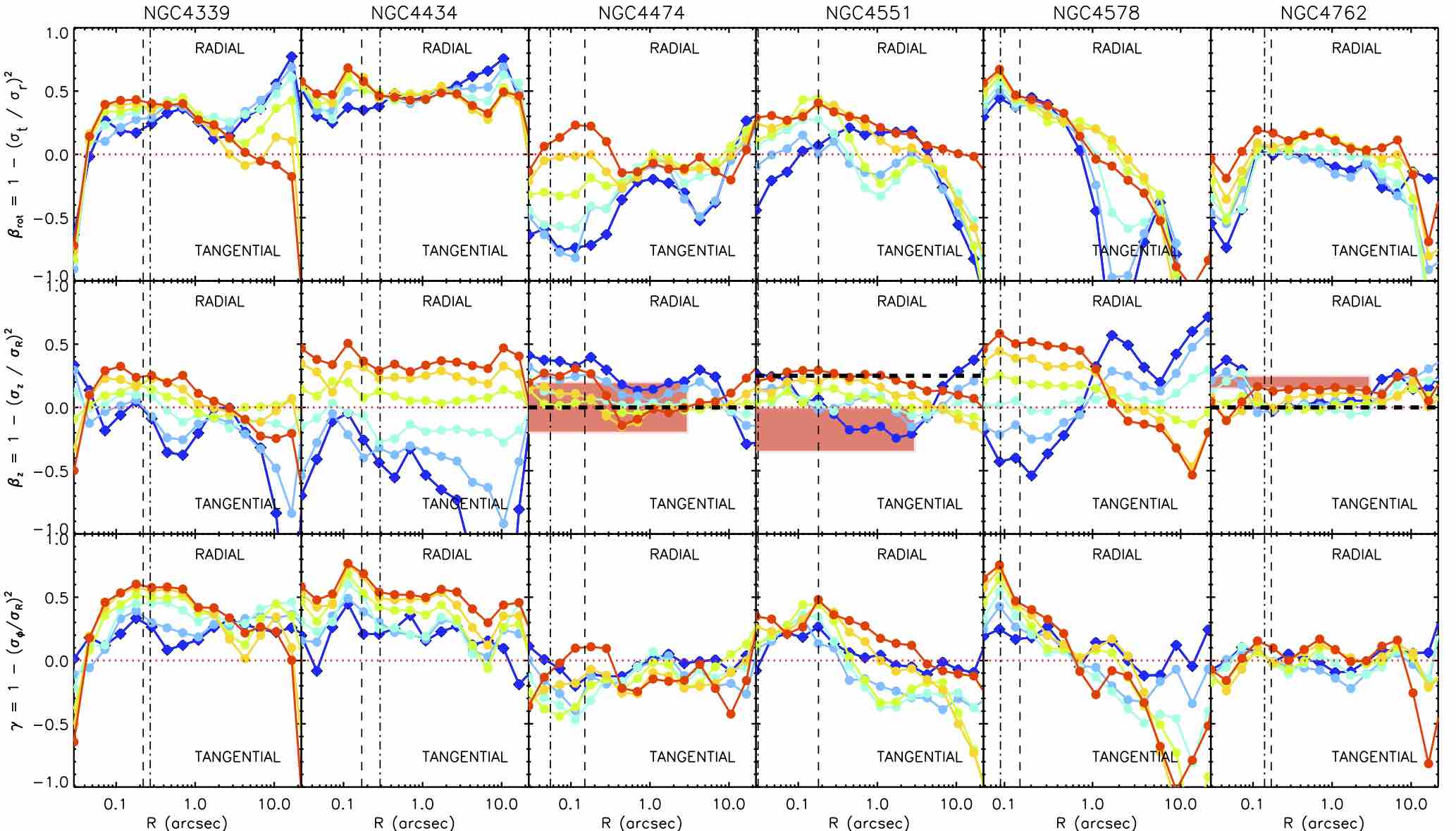
5.3 Orbital structure and the shape of the velocity ellipsoid
The internal velocity structure of galaxies is specified by the velocity dispersion tensor, which defines the spread in stellar velocities at every position. Since the velocity dispersion tensor is symmetric, it is possible to choose a set of orthogonal axes in which the tensor is diagonal. These diagonalized coordinate axes specify the velocity ellipsoid. The shape of the velocity ellipsoid, defined by the velocity dispersion along the principle axes, is a useful tool for describing the velocity structure of a system. An ‘isotropic’ system has all velocity dispersions equal, while an ‘anisotropic’ system is a system where the velocity dispersions along the principle axes mutually differ (Binney & Tremaine, 2008). The nature of the Schwarzschild modelling allows for a general investigation of the velocity ellipsoid, as a function of radius and height from the equatorial plane.
We estimate three anisotropy parameters, one in the spherical (, , ) and two in cylindrical (, , ) coordinate systems. First, we specify the ratio of radial to tangential velocity dispersion as , where , in spherical coordinates. In this case, the isotropic systems will have , while radially and tangentially anisotropic systems have positive or negative, respectively. This is a similar measure to that used in other works (e.g. Gebhardt et al., 2003; Cappellari et al., 2007; Gültekin et al., 2009a; Krajnović et al., 2009; Thomas et al., 2014), but it is best suited for spherical objects. The second anisotropy parameter is as in the JAM models. It defines the shape of the velocity ellipsoid in the meridional plane including its two symmetry axes (major and minor), assuming axisymmetry. An additional anisotropy parameter is , which describes the equatorial plane of the velocity ellipsoid. When or the cross-sections of the velocity ellipsoids are circles and we speak of an isotropic system. When or the orbital distribution is biased towards a radially anisotropy, and when or it is biased towards tangential anisotropy.
We show results for our galaxies in Fig 11, specifically for models with formally best-fitting black hole masses (for NGC 4474 and NGC 4551 we use the models with the upper limit black hole masses). While there are certain differences between the galaxies, a general conclusion is that models have nearly isotropic or mildly radially biased velocity ellipsoid throughout their bodies. In spherical coordinates, NGC 4339 and NGC 4434 seem to be somewhat more radially biased, while the velocity ellipsoid of NGC 4578 has a more complex structure, changing the shape along the major axis from a radially biased within 1″ to a tangentially biased shape beyond that radius. In more appropriate cylindrical coordinate system, essentially all galaxies are nearly isotropic, with NGC 4339, NGC 4434 and NGC 4578 showing a larger scatter in anisotropy across different polar angles defined in the meridional plane. Galaxies with the MBH upper limits show a tendency for radial anisotropy in the central regions. The same features can also be seen in the models of these galaxies assuming MBH below the upper limits
The Schwarzschild models of the three galaxies at low inclinations (NGC 4339, NGC 4434 and NGC 4578) show a larger spread in recovered radial anisotropy profiles, while models of galaxies at higher inclinations have less scatter. We do not investigate this in detail, but the effects are likely related to the difficulties in recovering the true properties of systems at low inclinations, as Schwarzschild models also suffer from the inclination–anisotropy degeneracy. We also compare the anisotropy parameter obtained from JAM and Schwarzschild models for galaxies with inclination larger than 60°. Galaxies with lower inclinations are in the regime of a strong degeneracy between inclination and anisotropy (Lablanche et al., 2012), therefore, we compare only galaxies at higher inclinations. We compare both the results of our JAM models which are restricted to the central and JAM models151515Anisotropy values for the full ATLAS3D sample are available on http://purl.org/atlas3d. of Cappellari et al. (2013a) which sample the full SAURON FoV. For both sets of models there is a rather good comparison with Schwarzschild results, except for NGC4551, for which the JAM models based on NIFS data only favour middy tangentially anisotropic solutions, but still consistent with isotropy. Schawarzschild models favour a more radially anisotropic solution, similar to the JAM models based on SAURON data. We note that this galaxy is seen at a lower inclination (°), which could also be a source of error in determination of the anisotropy.
For galaxies with firm black hole mass detections, we do not observe significant changes in the anisotropy parameters as one crosses the black hole SoI (dot–dashed line); the velocity anisotropy profiles remain mostly isotropic or mildly radially anisotropic. A mild change in anisotropy from isotropic to radial anisotropic, or a bias to radial anisotropy, is detectable in NGC 4474 and NGC 4551, galaxies with upper limits on black hole mass. We will come back to this issue in Section 5.4.
The lack of tangentially biased orbits in the region dominated by the gravitational potential of the black holes is consistent with the picture in which the tangential anisotropy is the consequence of the core scouring by interaction of binary black holes (Quinlan et al., 1995; Quinlan & Hernquist, 1997; Milosavljević & Merritt, 2001; Thomas et al., 2014). Such behaviour is expected for more massive galaxies and slow rotators in general which grow via relatively frequent dry merging (see review by Cappellari, 2016). The photometric shapes, the kinematics and the masses can rule out this kind of event in the mass assembly for our galaxies, and now we can also add the shapes of the velocity ellipsoids as evidence that the growth of the galaxies and their central black holes was not dominated by significant dissipation-less merging.
The evidence for an isotropic to mildly radially anisotropic orbital distribution seems, however, to be contrary to expectations for adiabatic growth of black holes or creation of central stellar disc from nuclear starbursts (e.g. Quinlan et al., 1995). The predictions are however done for a spherical system, and if one considers the parametrization for spherical coordinates (which might be more applicable for the vicinity of the black hole), our results are compatible with mild tangential anisotropy as predicted and found for other galaxies (e.g. see a compilation of Thomas et al., 2014).
5.4 Are there super-massive black holes in NGC 4474 and NGC 4551?
The two galaxies for which we constrain MBH to be smaller than we can resolve have unusual central dips in the velocity dispersion maps. Their radius is approximately 0.5″ for NGC 4474, and about 1″ for NGC 4551, or about 35 and 80 pc, respectively. These features have a crucial influence in the construction of the dynamical models. A black hole of M⊙ and a of 100 km/s at the distance of 16 Mpc (like for these two galaxies), would have an SoI of about 0.06″, which could, in principle, be detected, given our data resolution and the experience with similar data types and quality (both high resolution and large scale IFU data, Krajnović et al., 2009; Cappellari et al., 2010; Thater et al., 2017). Fig. 9, however, shows that this is not the case. For both galaxies it can be ruled out that black holes of such a mass are present. Furthermore, the projected angular size of the velocity dispersion dips are a factor of 10-20 larger than radius of the SoI for a M⊙ black hole. What are then the origins of central decreases in the velocity dispersion maps?
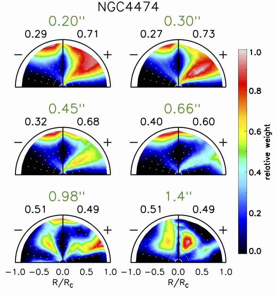
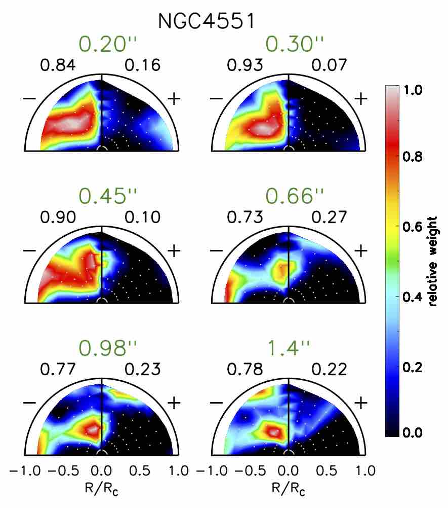
One possibility is that the dips in the velocity dispersion maps are caused by a specific stellar structure making a nuclear sub-component. The two galaxies are seen at different inclinations, NGC 4474 is almost edge on, and it has a prominent large-scale stellar disc. NGC 4551 is, however, at a moderate inclination of 65∘, which makes it difficult to recognize a large-scale disc morphology. Ferrarese et al. (2006), based on a sharp change in the ‘disciness’ parameter, , identified a nuclear disc in NGC 4551 seen at scales below 0.1″, but reported no such a structure in the case for NGC 4474, even though there is a similar behaviour of its . Even if the photometric feature in NGC 4551 on these scales is really confirmed as a disc, its size is smaller compared to the structure on the NIFS velocity dispersion maps, and it is difficult to make a direct link. Neither of the galaxies have noticeable dust, either filamentary or confined to a plane. Ellipticity of NGC 4474 is 0.15 at about 1″ and increases with a peak of 0.35 at 0.5″, before dropping to 0.13 in the centre. NGC 4551 is different in the sense that its ellipticity is relatively high (0.35) between 0.2 and 2″, but also drops to 0.2 in the centre. The rapid change of ellipticity may indicate the existence of components seen at different inclinations than the rest of the galaxy, but in the two cases the changes in ellipticity are quantitatively different while producing the same kinematic signature. Both galaxies have a central excess of light over a Sérsic fit to the full light radial profile, which for NGC 4474 is visible at radii smaller than 0.15″, while for NGC 4551 already at about 0.5″. These excesses are probably the only stellar nuclear structures which could be related to the observed dips in the kinematics.
Such structures may still correspond to stars that were once arranged in disc, if one considers the impact that minor merger events have on nuclear discs. Indeed, whereas such events easily disrupt the thin structure of discs such that they would no longer be recognized photometrically, the kinematic signature of the disc stars would survive such event, although the remnant disc may not be as dynamically cold as it originally was (Sarzi et al., 2015).
The total gravitational potential is traced by the second velocity moment, adequately approximated by a combination of the velocity dispersion and the mean rotational velocity. Therefore, in the case of a stellar disc, Vrms (or the second velocity moment), should not show a specific central feature, because the (increased) velocity and (decreased) velocity dispersions compensate. Vrms maps in Fig. 6 clearly show that this is not the case: dips in the Vrms maps are present and very similar to those seen in the velocity dispersion maps. Therefore, the morphology of the Vrms maps does not support the assumption that the kinematic dips are made by dynamically cold stellar structures such as nuclear discs.
In Fig. 12 we show the distribution of orbits in the central 1.5″ of both galaxies, covering larger regions than those displaying the velocity dispersion dips. We selected the formally best-fitting Schwarzschild models (with MBH of and M⊙ for NGC 4474 and NGC 4551 respectively), but orbital distributions are quantitatively the same for all models with black hole masses less than the derived upper limits. Each semicircle in Fig. 12 represents orbits of a given energy , while the other two integrals of motions defining an orbit are traced within the semicircle: the orbits of the highest are at the radius of the circular orbit (), while the orbits with increasing are increasingly more distant from the horizontal axis. Therefore, at a given energy, high angular momentum orbits, which are flat and build discs, are found in the corners of the semicircles, while orbits with high third integral are at the top of the semicircles, and build more spherical structures.
A striking feature of panels on Fig. 12, for both galaxies, is the lack of high angular momentum orbits confined to the disc plane. Orbits populating a disc should have a low third integral and be found close to the location of the circular orbit. To some extent these orbits are present in NGC 4551 around 0.5″ (seen on third and fourth hemispheres on Fig. 12) from the centre of the galaxy, but they do not extend closer to the assumed location of the black hole. The reason for this is seen on the Vrms map (Fig. 6), which shows increased values along the major axis at that radius (0.5″), and is evident on the maps of the mean velocity (Fig. 2) as the end points of the outer disc.
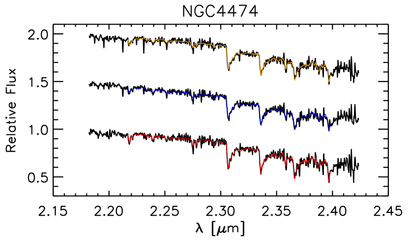
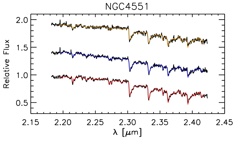
Based on stellar populations within the SAURON FoV, NGC 4474 and NGC 4551 do not seem to be significantly different from other galaxies in the sample. There is evidence for an intermediate age stellar population ( Gyr) within central 2–3″, but otherwise they have negative gradients in metallicity and ratios similar to those of other galaxies (Kuntschner, 2015; McDermid et al., 2015; Poci et al., 2017). The kinematic dips are seen only on the NIFS data and confined to the central 0.5″, a region fully within a fraction of the SAURON central pixel. Characterizing the stellar populations from NIR spectra is, however, more challenging (Silva et al., 2008; Lyubenova et al., 2008). As a test we selected three different regions in both galaxies: a central one encompassing central pixels, and two diametrically opposite regions centred on (0.7, 0.7″) and (-0.7, -0.7″) and approximately 0.2″ in radius. In this way all regions have similar S/rN after the pPXF fit. The spectra are shown on Fig. 13. We note that both NaI (2.20 m) and CaI (2.26 m) features seem to be deeper in the central spectra (for both galaxies), but we do not perform a detailed stellar population analysis. Instead, we fit the spectra with pPXF and record the templates (from GNIRS NIR stellar library of Winge et al., 2009) needed for the fit. For the central spectrum of NGC 4474 the fit required stars of the following types: F7III, G7III, K1V and K2III stars. The other two regions required these same stars and in addition G9III and K0IV stars. For the central spectrum of NGC 4551 the fit required stars of the following types: F7III, G8V, K1V and K2III stars. The other two regions required these same stars and in addition a G7III star. For both galaxies, pPXF fits are of the same quality and are able to reproduce all absorption features. Therefore, we conclude that if there are differences between the stellar population within and outside of the regions with kinematic dips, they are not significant for the observed stellar kinematics.
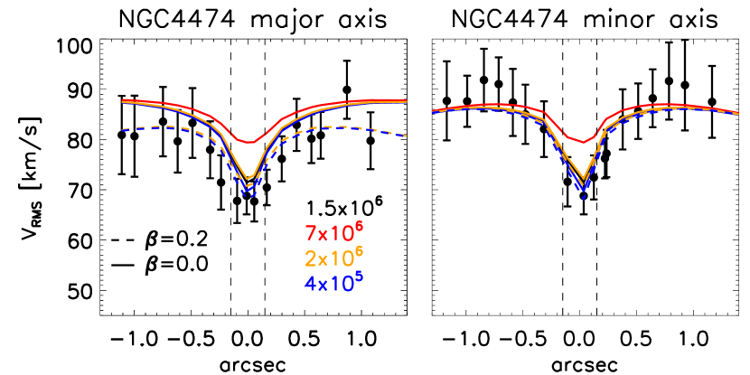
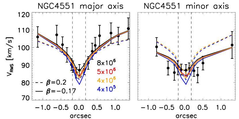
Even though we are not able to use NIR spectra to determine details of the stellar population properties within the velocity dispersion drops, we can consider what would be an effect of variable stellar populations within the NIFS FoV. For example, if IMF changes rapidly from a dwarf-rich (Salpeter) in the centre to a dwarf-poor (e.g. Chabrier) at the edge of the NIFS FoV, the M/L ratio of the stellar populations will drop by 0.25 dex (e.g. Bernardi et al., 2010). Our dynamical models assumed a constant M/L, where such as change in stellar populations M/L would be distributed between the dynamical M/L and MBH. Therefore, we run two tests using JAM models with varying M/Lpops ratios for both NGC 4474 and NGC 4551. In the first test, we assumed that the M/L of the stellar populations () decreases from a M/L based on dwarf-rich IMF in the centre to a based on dwarf-poor IMF at the edge of the NIFS FoV. In the second test we assumed an inverse change to , where the central was based on dwarf-poor IMF and the at the edge was based on dwarf-rich IMF. We introduced the change in the by fixing the based on Salpeter IMF (dwarf rich) to values from (Cappellari et al., 2013b), converted to our bands, and the based on Chabrier by subtracting 0.25 dex. The M/Lpops ratios changed between these two limiting values logarithmically for each Gaussian of the MGE model which cover the extent of the NIFS FoV.
We rerun grids of JAM models constrained by the Vrms from the NIFS data. For NGC 4474 there was no change in the estimate of MBH, only the upper limits changed. In the case of the dwarf-poor central IMF the MBH upper limit was higher than that obtained for constant in Section 4.3 by a factor of 1.4. Conversely, in the case of dwarf-rich central IMF the upper limit was smaller by a factor of 1.6 than the nominal one. Essentially, the grids were the same as in Fig. 5, with just a horizontal shift of the contours. We found similar results for NGC 4551, where the Fig. 5 grid already indicated a possible level detection of MBH. For dwarf-poor central IMF the models recovered an M M⊙. Models based on the dwarf-rich central IMF, however, constrained only an upper limit of M M⊙. In this case again the difference from the nominal models were from a factor of 1.5 to a factor of 4.
These results should take into account that recent studies (e.g. Dutton et al., 2013; La Barbera et al., 2016; van Dokkum et al., 2017) are finding evidence for a change in IMF which corresponds to dwarf-rich in the centre and dwarf-poor in outskirts, if any changes can be detected (e.g. McConnell et al., 2016). The consequence is that black holes in NGC 4474 and NGC 4551, if they are present, would be even less massive than what we constrain with our nominal models using a constant , while the MBH estimate based on the imposed lower central (due to Chabrier IMF) is not likely. Furthermore, these varying ratio tests indicate a level of the systematics on the estimate of MBH which is typically not taken into account; it seems every MBH should be considered uncertain to a factor of 1.5-2.
The absence of clear structural features (e.g. nuclear discs), which could support the central decreases in the velocity dispersion and Vrms maps, suggest that the origin of the dips is at least partially linked to the non-detection of the black holes. As shown by other galaxies in the sample, black holes exert influence on larger radii than the radii of their SoIs. Using the M scaling relation (e.g. Saglia et al., 2016), the predicted masses of black holes for NGC 4474 and NGC 4551 are and M⊙, respectively. Such black holes would have R″ and 0.025″, respectively, a factor 7-8 times smaller than the achieved resolution. In Fig. 14 we compare JAM models of various MBH with the data extracted along the major and minor axes. The models are not able to reproduce all points along both major and minor axes at the same time, but essentially all models are able to fit the dips in . By changing the anisotropy parameter, one can achieve locally better fits, but they are still not able to discriminate between various black hole models. NGC 4474 and NGC 4551 data have the lowest S/N and there are evidences of possible template mismatch. Given the uncertainties on the kinematics and the limited resolution achieved with the AO observations, only an upper limit can be given to black hole masses in these galaxies.
NGC 4474 and NGC 4551 have X-ray upper limits of and erg s-1, respectively (Gallo et al., 2010). These galaxies lack warm ionized gas in their nuclei and NGC 4551 is also not detected in the radio continuum with an upper limit of W Hz-1 at 5 GHz (Nyland et al., 2016). These black holes are dormant, and it is highly speculative to estimate their black hole masses from X-ray and radio observations of the nuclei. Using Gültekin et al. (2009c) relation between radio and X-ray flux and black hole mass, for NGC 4551 upper limits, we obtain M M⊙, about an order of magnitude larger than allowed by the models. The uncertainly on the accretion level prohibits a more robust estimate.
It is nevertheless interesting to consider a possibility that NGC 4474 and NGC 4551 are candidates for galaxies with significantly undermassive or no central black holes, joining a few more objects with stringent MBH upper limits below what is predicted by scaling relations, based on either unresolved or resolved nuclear ionised-gas, or stellar kinematics (e.g. Coccato et al., 2006; Beifiori et al., 2009; Gültekin et al., 2011).
If NGC 4474 and NGC 4551 have undermassive black holes, they are representative of galaxies where black holes did not co-evolve with hosts, perhaps due to low level and sporadic feeding (Kormendy & Ho, 2013). Among other scenarios, NGC 4474 and NGC 4551 might have never had black holes, or they lost them during one of the past merging events, when the black holes were kicked out of the galaxies. The first scenario is difficult to reconcile with current ideas about the quenching of star formation (e.g. Vogelsberger et al., 2014; Crain et al., 2015; King & Pounds, 2015). There are, however, several mechanism which could be invoked for the removal of the black holes (Batcheldor et al., 2010), of which the gravitational wave recoil originating in the merger of a binary black hole system seems the most favourable as it can provide recoil velocities in excess of 3000 km/s (e.g. Campanelli et al., 2007a; Lousto & Zlochower, 2011), adequate to eject black holes from galaxies (e.g. Campanelli et al., 2007b; Volonteri et al., 2010). The main difficulty with the second scenario is that such kicks should not occur often, requiring a special geometry and black hole spin alignment, mostly resulting in black holes oscillating around the centre of the gravitational potential instead of being completely ejected (e.g. Merritt et al., 2004; Gualandris & Merritt, 2008; Lousto et al., 2012).
If a black hole from NGC 4474 or NGC 4551 was kicked out of its host, the progenitor of the host had to go through a merger event which allowed for the creation of a binary black hole. This means that progenitors had to be of a similar mass (so that their black holes are of similar masses to about a factor of two). The light profiles of NGC 4474 or NGC 4551 show mild excesses in the centres, and these galaxies are fast rotators with large scale discs. A dry major merger, typically invoked for enabling a creation of a binary black hole (e.g. Kormendy et al., 2009), is therefore not a likely choice. Another possibility is that these galaxies first experienced a dry merger and lost their black holes followed by a subsequent accretion event that made the outer disc and the central light excess. A possible hybrid scenario is a variant to a scenario proposed by Krajnović et al. (2013b) to explain cores in fast rotator galaxies. The black hole binary was created during a wet merger, but the coalescence of black holes in this case was on a shorter time-scale than the duration of starbursts (see also Faber et al., 1997). As the starburst continued after the black holes merged and were ejected by the kick from the gravitational wave emission, it was able to create the nuclear excess of light. Both of these scenarios, like the scenario with no black holes to start with, leave open the question of how the star formation was quenched. The surroundings of these galaxies provide a possible solution. These galaxies are members of Virgo Cluster, and live in the densest environment compared with other galaxies in our sample (Cappellari et al., 2011b), implying that the (final) quenching of the star formation could have been purely environmental.
As outlined earlier (see Section 5.3), a merger of black holes should bias the orbital distribution towards tangential anisotropy. Fig. 12 shows that the Schwarzschild models require a mild increase in the radial anisotropy of the velocity tensor in the central 0.3″ for NGC 4474 (although an isotropic solution is also acceptable in this case) and NGC 4551. Parameterizing the anisotropy in spherical coordinates, NGC 4474 shows a tendency to tangential orbits, but the scatter is large and it is not possible to distinguish between trends for adiabatic black hole growth or core scouring. Taking all data together, we conclude that such orbital configurations within the scenario of the ejected black holes is possible only if the nuclear starburst is of longer duration than the merging of the black hole binary, and, therefore can replenish stars on radial orbits that were initially removed by the binary.
The evidence presented cannot prove the non-existence of central black holes in NGC 4474 and NGC 4551. The data support that these galaxies could harbour highly unusual black holes, about an order of magnitude smaller than the predictions. While it is difficult to choose between possible scenarios (a black hole that did not co-evolve, a black hole that was kicked out, or never having had a black hole at all), detecting the presence of very low-mass nuclear black holes will be achievable with the next generation of telescope facilities, such as the James Webb Space Telescope or from the ground-based Extremely Large Telescope.
6 Conclusion
We observed six ETGs (NGC 4339, NGC 4434, NGC 4474, NGC 4551, NGC 4578 and NGC 4762) selected from the ATLAS3D sample with NIFS LGS AO in order to determine the masses of the central black holes. Galaxies were selected to be fast rotators of relatively low mass ( M⊙, except NGC 4762 which is M⊙) and velocity dispersion within the effective radius of km/s ( km/s for NGC 4762). Four galaxies are members of the Virgo Cluster (at the distance of about 16 Mpc), while two are isolated objects at larger distance (at about 22 Mpc).
We extract the kinematics in the NIR and show that they are consistent with the optical observations with SAURON from the ATLAS3D survey. The spatial resolution achieved with the LGS AO is below 0.2″, allowing us to probe the stellar kinematics in the vicinity of the central black hole. We parameterize the light distributions of our galaxies using space- and ground-based imaging, and then construct the three-dimensional mass distribution assuming axisymmetry and inclinations derived in previous studies. We build two types of dynamical models: JAM, based on the Jeans equations allowing for a velocity anisotropy, and Schwarzschild models based on the superposition of orbits. The JAM models are only constrained by the high spatial resolution NIFS data, while Schwarzschild models use both large-scale SAURON data and NIFS data presented in this work. The two approaches give remarkably consistent results, in all but one galaxy the differences between JAM and Schwarzschild models are between , while for one galaxy the difference is just above confidence level. Both methods are able to constrain black hole masses for four galaxies, while for two galaxies the models favour black hole masses that are smaller than we can resolve.
Two of our galaxies (NGC 4339 and NGC 4434) have black hole masses that are more massive than the expectation from the latest M relation by about twice the reported scatter of the relation ( and M⊙, respectively, at confidence level). Two galaxies (NGC 4578 and NGC 4762) have black hole masses as predicted by the M relation ( and M⊙, respectively, at confidence level). The scatter between these measurements could be related to the differences in the feeding of the black holes, but there are no correlations with the type of internal structure (all have relatively high bulge Sérsic index and exponential discs) or the environment (objects above and on the relation from our sample comprise both isolated and cluster objects).
The data for two galaxies (NGC 4474 and NGC 4551) are consistent with not having central black holes (with upper limits of and M⊙, respectively, at confidence level). Their stellar velocity dispersion maps are characterized by large (0.5 and 1″, respectively) central declines. These cannot be attributed to nuclear discs as those are not visible in the light distribution, nor in the kinematics. The Schwarzschild models also do not require fast rotating discs to reproduce the data. Specifically, second velocity moments (), which trace the gravitational potential, also show distinct decreases in the central values. JAM models with MBH as predicted by the scaling relations ( and M⊙, respectively), which are nominally below our resolution, still produces too high central values, not compatible with the data. If there are central black holes in these galaxies they have masses less than a few M⊙. Our conjecture is that these are prime candidates for galaxies that lost their black holes, possibly due to gravitational recoils resulting from a coalescence of a black hole binary.
The nuclear orbital distribution for all our galaxies is consistent with being isotropic or mildly radially anisotropic. Given that our galaxies have Sérsic profiles or show excess of light in the nuclei, this is consistent with findings that tangentially anisotropic velocity ellipsoids in the vicinity of black holes are preferentially found in galaxies with cores (deficits of light). The mechanism for the excavation of the core via a black hole binary is linked with the removal of stars on radial orbits and modification of the orbital anisotropy. This means that our galaxies either did not experience a major dry merger (required for core excavation) or they went through a subsequent event that replenished the core. As our galaxies have old stellar populations this must have happened at large redshift (z). The galaxies which we consider candidates for not having black holes show a mild increase towards radial anisotropy within their nuclei. As their black holes were possibly kicked out by a recoil generated in the emission of gravitational waves, the coalescence of the black hole binary had to happen on a shorter time-scale than the nuclear starburst that refilled the excavated cores and changed the orbital anisotropy.
Acknowledgements
MC acknowledges support from a Royal Society University Research Fellowship. RMcD is the recipient of an Australian Research Council Future Fellowship (project number FT150100333). JF-B acknowledges support from grant AYA2016-77237-C3-1-P from the Spanish Ministry of Economy and Competitiveness (MINECO). Based on observations obtained at the Gemini Observatory, which is operated by the Association of Universities for Research in Astronomy, Inc., under a cooperative agreement with the NSF on behalf of the Gemini partnership: the National Science Foundation (United States), the National Research Council (Canada), CONICYT (Chile), Ministerio de Ciencia, Tecnologia e Innovación Productiva (Argentina), and Ministério da Ciência, Tecnologia e Inovação (Brazil). Based on observations made with the NASA/ESA Hubble Space Telescope, obtained from the data archive at the Space Telescope Science Institute. STScI is operated by the Association of Universities for Research in Astronomy, Inc. under NASA contract NAS 5-26555.
References
- Abazajian et al. (2009) Abazajian K. N., et al., 2009, ApJS, 182, 543
- Agarwal et al. (2013) Agarwal B., Davis A. J., Khochfar S., Natarajan P., Dunlop J. S., 2013, MNRAS, 432, 3438
- Agarwal et al. (2014) Agarwal B., Dalla Vecchia C., Johnson J. L., Khochfar S., Paardekooper J.-P., 2014, MNRAS, 443, 648
- Bacon et al. (2001) Bacon R., et al., 2001, MNRAS, 326, 23
- Barth et al. (2016) Barth A. J., Boizelle B. D., Darling J., Baker A. J., Buote D. A., Ho L. C., Walsh J. L., 2016, ApJ, 822, L28
- Batcheldor et al. (2010) Batcheldor D., Robinson A., Axon D. J., Perlman E. S., Merritt D., 2010, ApJ, 717, L6
- Beifiori et al. (2009) Beifiori A., Sarzi M., Corsini E. M., Dalla Bontà E., Pizzella A., Coccato L., Bertola F., 2009, ApJ, 692, 856
- Bernardi et al. (2007) Bernardi M., Sheth R. K., Tundo E., Hyde J. B., 2007, ApJ, 660, 267
- Bernardi et al. (2010) Bernardi M., Shankar F., Hyde J. B., Mei S., Marulli F., Sheth R. K., 2010, MNRAS, 404, 2087
- Binney & Tremaine (2008) Binney J., Tremaine S., 2008, Galactic dynamics. Princeton, NJ, Princeton University Press, 2008, second edition
- Blanton & Roweis (2007) Blanton M. R., Roweis S., 2007, AJ, 133, 734
- Boccas et al. (2006) Boccas M., et al., 2006, in Society of Photo-Optical Instrumentation Engineers (SPIE) Conference Series. , doi:10.1117/12.670842
- Bolatto et al. (2017) Bolatto A. D., et al., 2017, ApJ, 846, 159
- Campanelli et al. (2007a) Campanelli M., Lousto C. O., Zlochower Y., Merritt D., 2007a, Physical Review Letters, 98, 231102
- Campanelli et al. (2007b) Campanelli M., Lousto C., Zlochower Y., Merritt D., 2007b, ApJ, 659, L5
- Cappellari (2002) Cappellari M., 2002, MNRAS, 333, 400
- Cappellari (2008) Cappellari M., 2008, MNRAS, 390, 71
- Cappellari (2016) Cappellari M., 2016, ARA&A, 54, 597
- Cappellari (2017) Cappellari M., 2017, MNRAS, 466, 798
- Cappellari & Copin (2003) Cappellari M., Copin Y., 2003, MNRAS, 342, 345
- Cappellari & Emsellem (2004) Cappellari M., Emsellem E., 2004, PASP, 116, 138
- Cappellari & McDermid (2005) Cappellari M., McDermid R. M., 2005, Classical and Quantum Gravity, 22, 347
- Cappellari et al. (2006) Cappellari M., et al., 2006, MNRAS, 366, 1126
- Cappellari et al. (2007) Cappellari M., et al., 2007, MNRAS, 379, 418
- Cappellari et al. (2009) Cappellari M., Neumayer N., Reunanen J., van der Werf P. P., de Zeeuw P. T., Rix H.-W., 2009, MNRAS, 394, 660
- Cappellari et al. (2010) Cappellari M., et al., 2010, in Debattista V. P., Popescu C. C., eds, American Institute of Physics Conference Series Vol. 1240, American Institute of Physics Conference Series. pp 211–214 (arXiv:1001.3233), doi:10.1063/1.3458489
- Cappellari et al. (2011a) Cappellari M., et al., 2011a, MNRAS, 413, 813, Paper I
- Cappellari et al. (2011b) Cappellari M., et al., 2011b, MNRAS, 416, 1680, Paper VII
- Cappellari et al. (2012) Cappellari M., et al., 2012, Nature, 484, 485
- Cappellari et al. (2013a) Cappellari M., et al., 2013a, MNRAS, 432, 1709
- Cappellari et al. (2013b) Cappellari M., et al., 2013b, MNRAS, 432, 1862
- Chabrier (2003) Chabrier G., 2003, PASP, 115, 763
- Coccato et al. (2006) Coccato L., Sarzi M., Pizzella A., Corsini E. M., Dalla Bontà E., Bertola F., 2006, MNRAS, 366, 1050
- Conroy & van Dokkum (2012) Conroy C., van Dokkum P. G., 2012, ApJ, 760, 71
- Crain et al. (2015) Crain R. A., et al., 2015, MNRAS, 450, 1937
- Cretton & Emsellem (2004) Cretton N., Emsellem E., 2004, MNRAS, 347, L31
- Cretton et al. (1999) Cretton N., de Zeeuw P. T., van der Marel R. P., Rix H., 1999, ApJS, 124, 383
- Davis et al. (2013) Davis T. A., Bureau M., Cappellari M., Sarzi M., Blitz L., 2013, Nature, 494, 328
- Davis et al. (2017) Davis T. A., Bureau M., Onishi K., Cappellari M., Iguchi S., Sarzi M., 2017, MNRAS, 468, 4675
- Drehmer et al. (2015) Drehmer D. A., Storchi-Bergmann T., Ferrari F., Cappellari M., Riffel R. A., 2015, MNRAS, 450, 128
- Dutton et al. (2013) Dutton A. A., et al., 2013, MNRAS, 428, 3183
- Emsellem (2013) Emsellem E., 2013, MNRAS, 433, 1862
- Emsellem et al. (1994) Emsellem E., Monnet G., Bacon R., 1994, A&A, 285, 723
- Faber et al. (1997) Faber S. M., et al., 1997, AJ, 114, 1771
- Feldmeier-Krause et al. (2017) Feldmeier-Krause A., Zhu L., Neumayer N., van de Ven G., de Zeeuw P. T., Schödel R., 2017, MNRAS, 466, 4040
- Feldmeier et al. (2014) Feldmeier A., et al., 2014, A&A, 570, A2
- Ferrarese & Ford (2005) Ferrarese L., Ford H., 2005, Space Science Reviews, 116, 523
- Ferrarese & Merritt (2000) Ferrarese L., Merritt D., 2000, ApJ, 539, L9
- Ferrarese et al. (2006) Ferrarese L., et al., 2006, ApJS, 164, 334
- Ford et al. (1998) Ford H. C., et al., 1998, in Bely P. Y., Breckinridge J. B., eds, Society of Photo-Optical Instrumentation Engineers (SPIE) Conference Series Vol. 3356, Society of Photo-Optical Instrumentation Engineers (SPIE) Conference Series. pp 234–248
- Gallo et al. (2010) Gallo E., Treu T., Marshall P. J., Woo J.-H., Leipski C., Antonucci R., 2010, ApJ, 714, 25
- Gebhardt & Thomas (2009) Gebhardt K., Thomas J., 2009, ApJ, 700, 1690
- Gebhardt et al. (2000) Gebhardt K., et al., 2000, ApJ, 539, L13
- Gebhardt et al. (2003) Gebhardt K., et al., 2003, ApJ, 583, 92
- Gerhard (1993) Gerhard O. E., 1993, MNRAS, 265, 213
- Gerssen et al. (1997) Gerssen J., Kuijken K., Merrifield M. R., 1997, MNRAS, 288, 618
- Graham (2016) Graham A. W., 2016, Galactic Bulges, 418, 263
- Graham & Li (2009) Graham A. W., Li I.-h., 2009, ApJ, 698, 812
- Graham & Scott (2013) Graham A. W., Scott N., 2013, ApJ, 764, 151
- Graham et al. (2003) Graham A. W., Erwin P., Trujillo I., Asensio Ramos A., 2003, AJ, 125, 2951
- Graham et al. (2011) Graham A. W., Onken C. A., Athanassoula E., Combes F., 2011, MNRAS, 412, 2211
- Greene et al. (2010) Greene J. E., et al., 2010, ApJ, 721, 26
- Greene et al. (2016) Greene J. E., et al., 2016, ApJ, 826, L32
- Gualandris & Merritt (2008) Gualandris A., Merritt D., 2008, ApJ, 678, 780
- Gültekin et al. (2009a) Gültekin K., et al., 2009a, ApJ, 695, 1577
- Gültekin et al. (2009b) Gültekin K., et al., 2009b, ApJ, 698, 198
- Gültekin et al. (2009c) Gültekin K., Cackett E. M., Miller J. M., Di Matteo T., Markoff S., Richstone D. O., 2009c, ApJ, 706, 404
- Gültekin et al. (2011) Gültekin K., Richstone D. O., Gebhardt K., Faber S. M., Lauer T. R., Bender R., Kormendy J., Pinkney J., 2011, ApJ, 741, 38
- Haario et al. (2001) Haario H., Saksman E., Tamminen J., 2001, Bernoulli, 7, 223
- Häring-Neumayer et al. (2006) Häring-Neumayer N., Cappellari M., Rix H.-W., Hartung M., Prieto M. A., Meisenheimer K., Lenzen R., 2006, ApJ, 643, 226
- Holtzman et al. (1995) Holtzman J. A., Burrows C. J., Casertano S., Hester J. J., Trauger J. T., Watson A. M., Worthey G., 1995, PASP, 107, 1065
- Houghton et al. (2006) Houghton R. C. W., Magorrian J., Sarzi M., Thatte N., Davies R. L., Krajnović D., 2006, MNRAS, 367, 2
- Hu (2008) Hu J., 2008, MNRAS, 386, 2242
- Jarrett et al. (2000) Jarrett T. H., Chester T., Cutri R., Schneider S., Skrutskie M., Huchra J. P., 2000, AJ, 119, 2498
- Jeans (1922) Jeans J. H., 1922, MNRAS, 82, 132
- Khochfar et al. (2011) Khochfar S., et al., 2011, MNRAS, 417, 845, Paper VIII
- King & Pounds (2015) King A., Pounds K., 2015, ARA&A, 53, 115
- Kormendy & Ho (2013) Kormendy J., Ho L. C., 2013, ARA&A, 51, 511
- Kormendy et al. (2009) Kormendy J., Fisher D. B., Cornell M. E., Bender R., 2009, ApJS, 182, 216
- Kormendy et al. (2011) Kormendy J., Bender R., Cornell M. E., 2011, Nature, 469, 374
- Krajnović et al. (2005) Krajnović D., Cappellari M., Emsellem E., McDermid R. M., de Zeeuw P. T., 2005, MNRAS, 357, 1113
- Krajnović et al. (2009) Krajnović D., McDermid R. M., Cappellari M., Davies R. L., 2009, MNRAS, 399, 1839
- Krajnović et al. (2011) Krajnović D., et al., 2011, MNRAS, 414, 2923, Paper II
- Krajnović et al. (2013a) Krajnović D., et al., 2013a, MNRAS, 432, 1768
- Krajnović et al. (2013b) Krajnović D., et al., 2013b, MNRAS, 433, 2812
- Krajnović et al. (2017) Krajnović D., Cappellari M., McDermid R. M., 2017, preprint, (arXiv:1707.04274)
- Krist et al. (2011) Krist J. E., Hook R. N., Stoehr F., 2011, in Society of Photo-Optical Instrumentation Engineers (SPIE) Conference Series. , doi:10.1117/12.892762
- Kroupa (2002) Kroupa P., 2002, Science, 295, 82
- Kuntschner (2015) Kuntschner H., 2015, in Cappellari M., Courteau S., eds, IAU Symposium Vol. 311, Galaxy Masses as Constraints of Formation Models. pp 53–56, doi:10.1017/S1743921315003385
- Kuo et al. (2011) Kuo C. Y., et al., 2011, ApJ, 727, 20
- Kurucz (1991) Kurucz R. L., 1991, in Philip A. G. D., Upgren A. R., Janes K. A., eds, Precision Photometry: Astrophysics of the Galaxy. Davis Press, Schenectady, NY, p. 27
- La Barbera et al. (2016) La Barbera F., Vazdekis A., Ferreras I., Pasquali A., Cappellari M., Martín-Navarro I., Schönebeck F., Falcón-Barroso J., 2016, MNRAS, 457, 1468
- Lablanche et al. (2012) Lablanche P.-Y., et al., 2012, MNRAS, 424, 1495
- Lauer et al. (2007) Lauer T. R., et al., 2007, ApJ, 662, 808
- Leung et al. (2018) Leung G. Y. C., et al., 2018, Monthly Notices of the Royal Astronomical Society, p. sty288
- Li et al. (2016) Li H., Li R., Mao S., Xu D., Long R. J., Emsellem E., 2016, MNRAS, 455, 3680
- Livingston & Wallace (1991) Livingston W., Wallace L., 1991, An atlas of the solar spectrum in the infrared from 1850 to 9000 cm-1 (1.1 to 5.4 micrometer). NSO Technical Report, Tucson: National Solar Observatory, National Optical Astronomy Observatory, 1991
- Lousto & Zlochower (2011) Lousto C. O., Zlochower Y., 2011, Phys. Rev. D, 83, 024003
- Lousto et al. (2012) Lousto C. O., Zlochower Y., Dotti M., Volonteri M., 2012, Phys. Rev. D, 85, 084015
- Lyubenova et al. (2008) Lyubenova M., Kuntschner H., Silva D. R., 2008, A&A, 485, 425
- Magorrian et al. (1998) Magorrian J., et al., 1998, AJ, 115, 2285
- Mazzalay et al. (2016) Mazzalay X., Thomas J., Saglia R. P., Wegner G. A., Bender R., Erwin P., Fabricius M. H., Rusli S. P., 2016, MNRAS, 462, 2847
- McConnell & Ma (2013) McConnell N. J., Ma C.-P., 2013, ApJ, 764, 184
- McConnell et al. (2011) McConnell N. J., Ma C.-P., Gebhardt K., Wright S. A., Murphy J. D., Lauer T. R., Graham J. R., Richstone D. O., 2011, Nature, 480, 215
- McConnell et al. (2012) McConnell N. J., Ma C.-P., Murphy J. D., Gebhardt K., Lauer T. R., Graham J. R., Wright S. A., Richstone D. O., 2012, ApJ, 756, 179
- McConnell et al. (2016) McConnell N. J., Lu J. R., Mann A. W., 2016, ApJ, 821, 39
- McDermid et al. (2014) McDermid R. M., et al., 2014, ApJ, 792, L37
- McDermid et al. (2015) McDermid R. M., et al., 2015, MNRAS, 448, 3484
- McGregor et al. (2003) McGregor P. J., et al., 2003, in Iye M., Moorwood A. F. M., eds, Proc. SPIEVol. 4841, Instrument Design and Performance for Optical/Infrared Ground-based Telescopes. pp 1581–1591, doi:10.1117/12.459448
- Merritt et al. (2004) Merritt D., Milosavljević M., Favata M., Hughes S. A., Holz D. E., 2004, ApJ, 607, L9
- Metropolis et al. (1953) Metropolis N., Rosenbluth A. W., Rosenbluth M. N., Teller A. H., Teller E., 1953, J. Chem. Phys., 21, 1087
- Milosavljević & Merritt (2001) Milosavljević M., Merritt D., 2001, ApJ, 563, 34
- Mitzkus et al. (2017) Mitzkus M., Cappellari M., Walcher C. J., 2017, MNRAS, 464, 4789
- Monnet et al. (1992) Monnet G., Bacon R., Emsellem E., 1992, A&A, 253, 366
- Neumayer et al. (2007) Neumayer N., Cappellari M., Reunanen J., Rix H.-W., van der Werf P. P., de Zeeuw P. T., Davies R. I., 2007, ApJ, 671, 1329
- Nowak et al. (2007) Nowak N., Saglia R. P., Thomas J., Bender R., Pannella M., Gebhardt K., Davies R. I., 2007, MNRAS, 379, 909
- Nyland et al. (2016) Nyland K., et al., 2016, MNRAS, 458, 2221
- Onishi et al. (2015) Onishi K., Iguchi S., Sheth K., Kohno K., 2015, ApJ, 806, 39
- Poci et al. (2017) Poci A., Cappellari M., McDermid R. M., 2017, MNRAS, 467, 1397
- Quinlan & Hernquist (1997) Quinlan G. D., Hernquist L., 1997, New Astronomy, 2, 533
- Quinlan et al. (1995) Quinlan G. D., Hernquist L., Sigurdsson S., 1995, ApJ, 440, 554
- Richstone & Tremaine (1988) Richstone D. O., Tremaine S., 1988, ApJ, 327, 82
- Rix et al. (1997) Rix H., de Zeeuw P. T., Cretton N., van der Marel R. P., Carollo C. M., 1997, ApJ, 488, 702
- Rusli et al. (2013) Rusli S. P., et al., 2013, AJ, 146, 45
- Rybicki (1987) Rybicki G. B., 1987, in IAU Symp. 127: Structure and Dynamics of Elliptical Galaxies. p. 397
- Saglia et al. (2016) Saglia R. P., et al., 2016, ApJ, 818, 47
- Salpeter (1955) Salpeter E. E., 1955, ApJ, 121, 161
- Sánchez-Blázquez et al. (2006) Sánchez-Blázquez P., et al., 2006, MNRAS, 371, 703
- Sarzi et al. (2015) Sarzi M., Ledo H. R., Dotti M., 2015, MNRAS, 453, 1070
- Savorgnan (2016) Savorgnan G. A. D., 2016, ApJ, 821, 88
- Schaye et al. (2015) Schaye J., et al., 2015, MNRAS, 446, 521
- Schlafly & Finkbeiner (2011) Schlafly E. F., Finkbeiner D. P., 2011, ApJ, 737, 103
- Schulze & Gebhardt (2011) Schulze A., Gebhardt K., 2011, ApJ, 729, 21
- Schwarzschild (1979) Schwarzschild M., 1979, ApJ, 232, 236
- Scott et al. (2013a) Scott N., et al., 2013a, MNRAS, 432, 1894
- Scott et al. (2013b) Scott N., Graham A. W., Schombert J., 2013b, ApJ, 768, 76
- Sérsic (1968) Sérsic J. L., 1968, Atlas de galaxias australes. Cordoba, Argentina: Observatorio Astronomico, 1968
- Seth et al. (2014) Seth A. C., et al., 2014, Nature, 513, 398
- Shankar et al. (2016) Shankar F., et al., 2016, MNRAS, 460, 3119
- Shapiro et al. (2006) Shapiro K. L., Cappellari M., de Zeeuw T., McDermid R. M., Gebhardt K., van den Bosch R. C. E., Statler T. S., 2006, MNRAS, 370, 559
- Silva et al. (2008) Silva D. R., Kuntschner H., Lyubenova M., 2008, ApJ, 674, 194
- Siopis et al. (2009) Siopis C., et al., 2009, ApJ, 693, 946
- Sirianni et al. (2005) Sirianni M., et al., 2005, PASP, 117, 1049
- Spiniello et al. (2014) Spiniello C., Trager S., Koopmans L. V. E., Conroy C., 2014, MNRAS, 438, 1483
- Thater et al. (2017) Thater S., et al., 2017, A&A, 597, A18
- Thomas et al. (2004) Thomas J., Saglia R. P., Bender R., Thomas D., Gebhardt K., Magorrian J., Richstone D., 2004, MNRAS, 353, 391
- Thomas et al. (2011) Thomas J., et al., 2011, MNRAS, 415, 545
- Thomas et al. (2014) Thomas J., Saglia R. P., Bender R., Erwin P., Fabricius M., 2014, ApJ, 782, 39
- Thomas et al. (2016) Thomas J., Ma C.-P., McConnell N. J., Greene J. E., Blakeslee J. P., Janish R., 2016, Nature, 532, 340
- Tremaine et al. (2002) Tremaine S., et al., 2002, ApJ, 574, 740
- Valluri et al. (2004) Valluri M., Merritt D., Emsellem E., 2004, ApJ, 602, 66
- Verolme et al. (2002) Verolme E. K., et al., 2002, MNRAS, 335, 517
- Vogelsberger et al. (2014) Vogelsberger M., et al., 2014, MNRAS, 444, 1518
- Volonteri et al. (2010) Volonteri M., Gültekin K., Dotti M., 2010, MNRAS, 404, 2143
- Walsh et al. (2012) Walsh J. L., van den Bosch R. C. E., Barth A. J., Sarzi M., 2012, ApJ, 753, 79
- Walsh et al. (2013) Walsh J. L., Barth A. J., Ho L. C., Sarzi M., 2013, ApJ, 770, 86
- Walsh et al. (2016) Walsh J. L., van den Bosch R. C. E., Gebhardt K., Yıldırım A., Richstone D. O., Gültekin K., Husemann B., 2016, ApJ, 817, 2
- Winge et al. (2009) Winge C., Riffel R. A., Storchi-Bergmann T., 2009, ApJS, 185, 186
- Worthey (1994) Worthey G., 1994, ApJS, 95, 107
- Yıldırım et al. (2015) Yıldırım A., van den Bosch R. C. E., van de Ven G., Husemann B., Lyubenova M., Walsh J. L., Gebhardt K., Gültekin K., 2015, MNRAS, 452, 1792
- Zhu et al. (2018) Zhu L., et al., 2018, MNRAS, 473, 3000
- de Zeeuw (2001) de Zeeuw P. T., 2001, in Black Holes in Binaries and Galactic Nuclei. pp 78–+
- van Dokkum & Conroy (2010) van Dokkum P. G., Conroy C., 2010, Nature, 468, 940
- van Dokkum et al. (2017) van Dokkum P., Conroy C., Villaume A., Brodie J., Romanowsky A. J., 2017, ApJ, 841, 68
- van den Bosch (2016) van den Bosch R. C. E., 2016, ApJ, 831, 134
- van den Bosch & de Zeeuw (2010) van den Bosch R. C. E., de Zeeuw P. T., 2010, MNRAS, 401, 1770
- van den Bosch & van de Ven (2009) van den Bosch R. C. E., van de Ven G., 2009, MNRAS, 398, 1117
- van den Bosch et al. (2008) van den Bosch R. C. E., van de Ven G., Verolme E. K., Cappellari M., de Zeeuw P. T., 2008, MNRAS, 385, 647
- van den Bosch et al. (2012) van den Bosch R. C. E., Gebhardt K., Gültekin K., van de Ven G., van der Wel A., Walsh J. L., 2012, Nature, 491, 729
- van der Marel & Franx (1993) van der Marel R. P., Franx M., 1993, ApJ, 407, 525
- van der Marel et al. (1998) van der Marel R. P., Cretton N., de Zeeuw P. T., Rix H., 1998, ApJ, 493, 613
Appendix A An illustrative case of NGC 1277
NGC 1277 is a compact galaxy for which the Schwarzschild model of van den Bosch et al. (2012), based on seeing-limited (long-slit) stellar kinematics, initially indicated a significantly larger black hole (M M⊙) than predicted by the M relation, highlighting the galaxy as one of the most distant outliers from the black hole scaling relations. For the purpose of this section, the Schwarzschild models of van den Bosch et al. predicted a black hole in NGC 1277 much larger than the value of M M⊙ (Emsellem, 2013). The later models are based on an -body realization having the first and second moments identical to a JAM model (when computed via equations 19 – 21 in Cappellari, 2008), and were constrained with the same data as the Schwarzschild models. Emsellem (2013) did not explore the full parameter space, but assumed instead a fixed inclination (75°, as in van den Bosch et al., 2012), and an ad hoc value =10. This discrepancy of results made NGC 1277 the only galaxy for which JAM-like- and Schwarzschild-based MBH estimates did not agree. NGC 1277 is a fast rotating galaxy, consistent with axisymmetry (Yıldırım et al., 2015) and as such is suitable for JAM modelling. The seeing-limited JAM-equivalent black hole estimate was also established by the Schwarzschild models of Walsh et al. (2016) finding M M⊙ ( formal errors ignoring systematics) when using high-resolution NIFS IFU data.
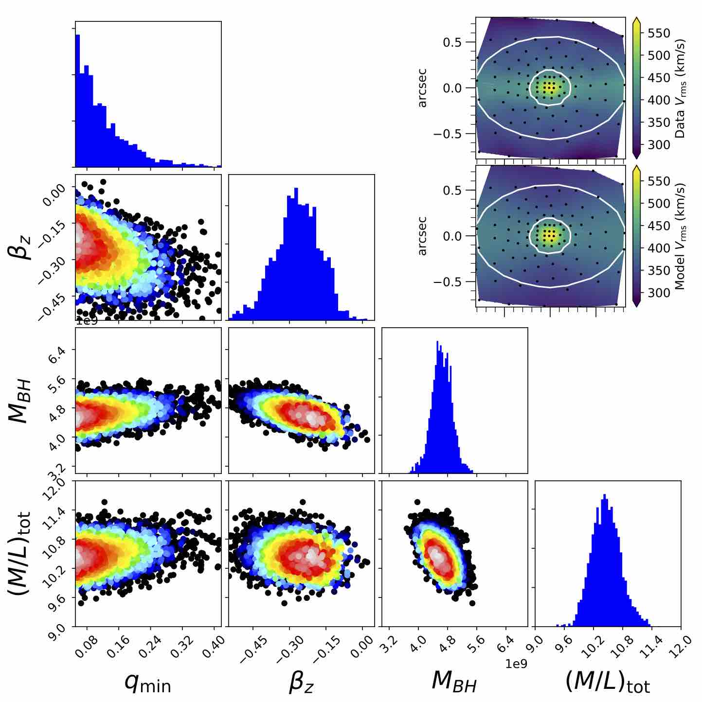
As an additional test for this paper, we used the JAM method to fit a mass-follows-light model to NGC 1277 using the same published IFU kinematics and errors of Walsh et al. (2016), where we defined , ignoring and . For maximum consistency, we adopted their published PSF parametrization, distance, and the same MGE model from van den Bosch et al. (2012). We fit for the inclination (parameterized as axial ratio , which is the intrinsic axial ratio of the flattest Gaussian in the MGE), anisotropy , total and MBH in a Bayesian framework. The calculation of the posterior probability distribution is done using the adaptive Metropolis et al. (1953) algorithm of Haario et al. (2001). This algorithm, while very efficient, is strictly speaking non-Markovian, but it has the correct ergodic properties and can be used to estimate the posterior distribution as in standard Markov chain Monte Carlo method. We assumed ignorant (constant) priors on all model parameters. The corner plots of the probability distribution for the non-linear model parameters are shown in Fig 15. The data model comparison is shown in the upper-right corner of Fig. 15. Our best-fitting model has M M⊙, , ( formal errors), and . This quantity gives the best fitting inclination (using equation 14 from Cappellari, 2008) of . Within the level this value is consistent with 75°, the assumed inclination in van den Bosch et al. (2012, based on a dust ring), and subsequently used in all other above mentioned papers. The black hole mass is consistent with Walsh et al. (2016), while their stellar = and total = 9.5 (Walsh, private communication), are somewhat smaller, but still within the uncertainties with our estimates. The velocity anisotropy in the spherical coordinate system of NGC 1277 is published in Yıldırım et al. (2015) based on Schwarzschild models of large-scale data. While their anisotropy cannot be directly compared with JAM’s in the cylindrical coordinates, we note that in both cases the models favour tangentially anisotropic velocities. This adds NGC 1277 to those galaxies that show consistent results between the Schwarzschild and JAM modelling, in this case, for the first time when using the same data.

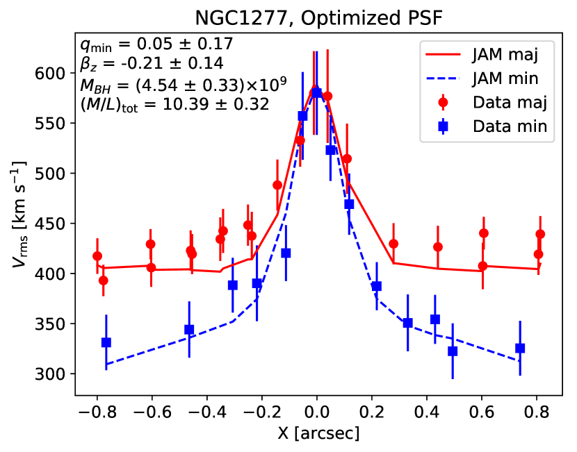
Looking for a more illustrative comparison between the data and the model we show cuts along the major and the minor axes on the top panel of Fig. 16. The model seems not to be able to reproduce the central peak in the . Similar disagreement can also be seen on fig. 4 of Walsh et al. (2016). A better fit can be achieved for a small change of the assumed PSF parameters. We changed the FWHM of the inner Gaussian component (of two Gaussian parametrization) from the 0.07″, preferred by Walsh et al. (2016), to 0.05″. This change is within the errors one can expect on the determination of the PSF (as also shown in this paper). The new PSF allows JAM model to fit essentially all data points (extracted along the major and minor axes on the figure) as is shown on the bottom panel of Fig. 16, while the change in the black hole mass and the anisotropy is essentially negligible (M M⊙ and ), and still fully consistent with the uncertainties quoted by Walsh et al. (2016).
While NGC 1277 is a more massive galaxy that those presented in this paper, its properties are in many ways similar to those of our galaxies (e.g. disc-dominated fast rotators). Therefore, it is reassuring that even for this galaxy (with initial contradictory claims) consistent black hole massed are recovered when the same, high-quality data are used, with two vastly different modelling techniques.
Appendix B Parametrisation of the PSFs
In Table 6 we show MGE parameters describing the PSF of the HST images, which were used for comparison with the NIFS reconstructed images and the determination of the NIFS PSF. In Fig. 6 we show the comparison along two axis between the NIFS reconstructed images and the HST convolved by the best-fitting PSF listed in Table 3.
Notes – For each galaxy the PSF is parameterized by 5–7 circular Gaussians. The ‘Norm’ column has the normalization of the Gaussian (such that the sum it equal to unity) and the ‘’ column has the dispersion of the Gaussian given in pixels. The conversion factor to physical units for WPFC2 is 0.0445 pixels per arcsec and for ACS is 0.05 pixels per arcsec.
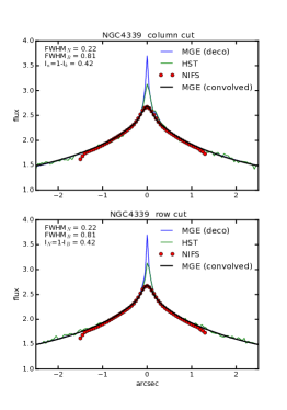
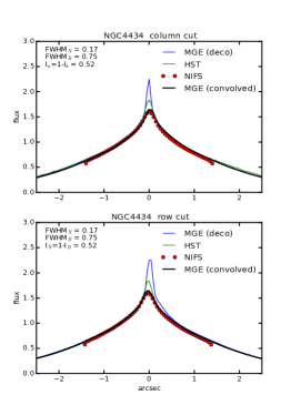
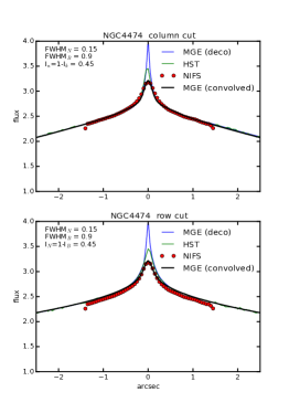
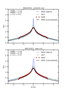
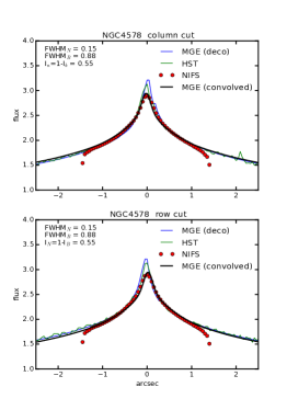
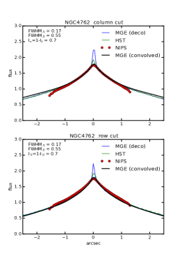
Appendix C SAURON kinematics
The extraction of SAURON kinematics161616Available from http://purl.org/atlas3d was presented in Cappellari et al. (2011a) and the velocity maps of our galaxies were already shown in Krajnović et al. (2011). Here, for completeness, we show the maps of the mean velocity, the velocity dispersion, and the and Gauss-Hermite moments, characterizing the full LOSVD. Typical error on the SAURON kinematics is noted in Table 4. Note that these maps are different from those shown in Appendix E as the data there were symmetrized for the modelling.
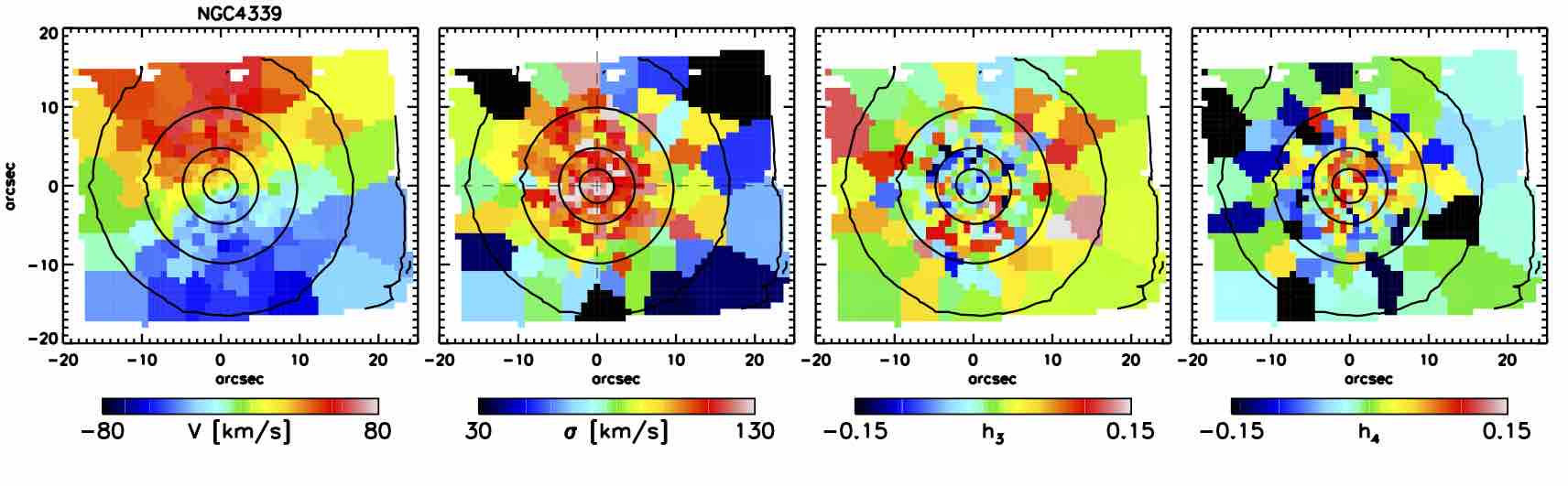
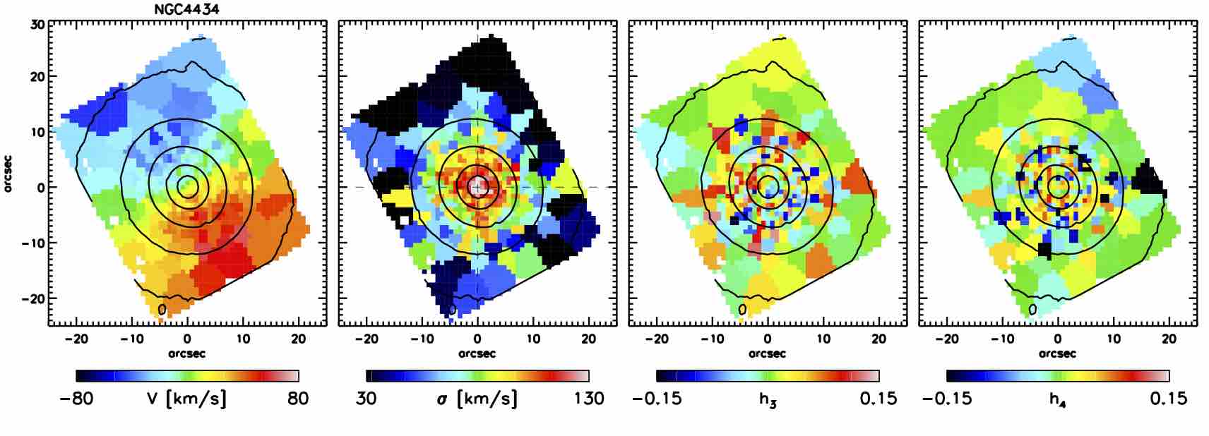
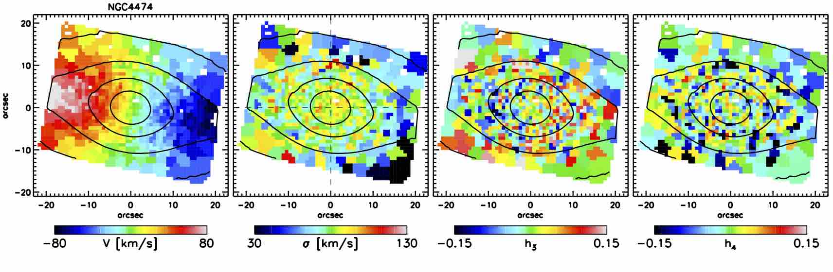
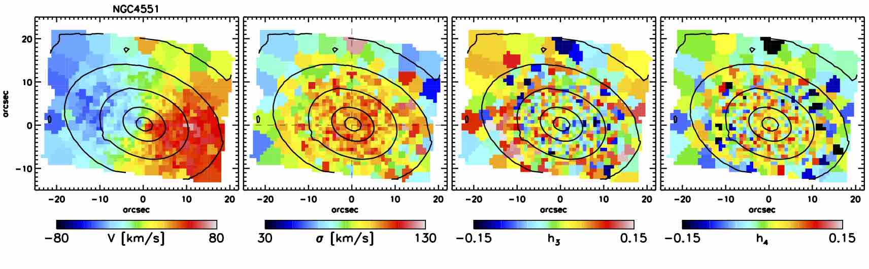

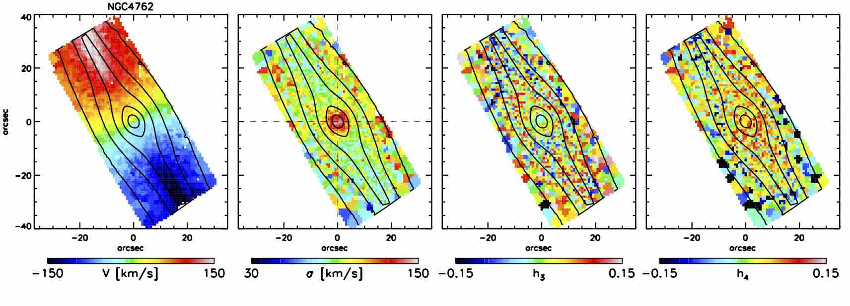
Appendix D MGE parametrization of the light distributions of sample galaxies
Notes: Galaxies from the ACS data are calibrated to the AB magnitude system (F450W band), while WFPC2 are on Vega system (Johnson R).
Appendix E Comparison of the Schwarzschild dynamical models with the symmetrised data