Efficient Bandwidth Estimation in Two-dimensional Filtered Backprojection Reconstruction

Abstract

A generalized cross-validation approach to estimate the reconstruction filter bandwidth in two-dimensional Filtered Backprojection is presented. The method writes the reconstruction equation in equivalent backprojected filtering form, derives results on eigendecomposition of symmetric two-dimensional circulant matrices and applies them to make bandwidth estimation a computationally efficient operation within the context of standard backprojected filtering reconstruction. Performance evaluations on a wide range of simulated emission tomography experiments give promising results. The superior performance holds at both low and high total expected counts, pointing to the method’s applicability even in weaker signal-noise situations. The approach also applies to the more general class of elliptically symmetric filters, with reconstruction performance often better than even that obtained with the true optimal radially symmetric filter.

I Introduction

Filtered Backprojection (FBP) [1, 2, 3] is commonly used in tomographic reconstruction where the goal is to estimate an object or emitting source distribution from its degraded linear projections that have been recorded by an appropriately designed set of detectors [4, 5, 6]. Such scenarios arise in areas such as astronomy  [7, 8, 9], materials science and non-destructive evaluation [10, 11, 12, 13, 14], electron microscopy [15] and tomosynthesis [16] or in object detection with security scanners [17]. A popular application is in emission tomography imaging such as Single Photon Emission Computed Tomography (SPECT) or Positron Emission Tomography (PET) [18, 19, 20, 21] that forms the primary setting for this article. The challenges in emission tomography inherent in the dosimetry constraints and the Poisson distribution of the sinogram emissions have meant the development of sophisticated statistical methods [22, 23, 24, 25, 26, 27]. Nevertheless, the computationally fast FBP is still very commonly used. Further, many of the gains associated with some of the sophisticated methods are typically in background regions and easily recovered by a quick postprocessing of the reconstructions [28, 29]. Also, three-dimensional (3D) PET reconstructions are often obtained from 2D sinograms acquired with septa in place or with Fourier Rebinning (FORE) [30, 31, 32]. However, FBP reconstruction is generally accompanied by smoothing that involves a bandwidth or resolution size parameter, often specified in terms of its full-width-at-half-maximum (FWHM), that must ideally be optimally set to get spatially consistent reconstructions. Similar to nonparametric function estimation in statistics, the quality of reconstruction is evaluated by, for instance, the squared error loss function [33, 34, 35, 36, 37].

Data-dependent unbiased risk estimation techniques [38, 39] – with practical modifications [40] to adjust for the extra-Poisson variation in corrected PET data – have been developed. The methodology is interpretable as a form of cross-validation (CV). Many practitioners however forego bandwidth selection schemes that involve additional steps beyond reconstruction, and instead either use a value that is fixed or visually chosen and typically undersmooths reconstructions.

The use of CV [41, 42] and the rotationally invariant Generalized CV (GCV) [43] is quite prevalent for bandwidth selection in nonparametric function estimation [44] and image restoration [45, 46, 47]. For moderate sample sizes, CV-obtained bandwidth parameters yield the best smoothed linear ridge and nonparametric regression estimators [48]. In image deblurring where a degraded version of the true image after convolving via a point-spread function is observed, [49] and [46] provide optimal GCV bandwidths that usually perform well [49] – howbeit see  [50] for examples of undersmoothing – but are impractical to obtain in tomographic applications because they require indirect function estimation (see Section 4.1 of [45]). Consequently, Section II of this article shows that the singular value decomposition (SVD) of the reconstruction (in matrix notation) can be readily obtained from results on symmetric one-dimensional (1D) and 2D circulant matrices, which are also derived here. The Predicted Residual Sums of Squares (PRESS) are then very easily obtained in a similar spirit to [43] and practically minimized en route to FBP reconstruction to obtain the GCV-estimated bandwidth. The methodology is evaluated on simulated 2D phantom data in Section III. Our implementation and results show that GCV selection and PET reconstruction can be carried out in less than a second, achieving an integrated squared error that is very close to the ideal. Moreover, our optimal reconstructions have the maximum relative benefits at lower rates of emissions. Further, the methodology can be used to optimally select parameters in the wider class of elliptically symmetric 2D kernel smoothers. Postprocessing proposed in [28] further improves reconstruction quality by removing negative artifacts. Our article concludes with some discussion including areas that could benefit from further extensions of our development. This paper also has a supplement.

II Theory and Methods

II-A Background and Preliminaries

Let $y_{r\theta}$ be the attenutation-, scatter- and randoms-corrected sinogram measurement along the line of response (LOR) indexed by $(r,\theta)$, $r=1,2,\ldots,R;\theta=1,2\ldots,\Theta$. Assume that the sinogram has $n=R\Theta(>p)$ LORs. Suppose that we use FBP to reconstruct the underlying source distribution in an imaging grid of $p$ pixels. In convolution form, the $i$th FBP-reconstructed pixel value, for $i=1,2,\ldots,p$, is

$$\hat{\lambda}_{i}^{h}=\sum_{\theta=1}^{\Theta}\sum_{r=1}^{R}e_{h}(x_{i}\cos\theta+y_{i}\sin\theta-r)y_{r\theta}.$$ (1)

Here, $e_{h}(\cdot)$ is the convolution filter with FWHM $h$. The summation over $r$ is a convolution and efficiently achieved though a series of 1D discrete Fast Fourier Transforms (FFT) and linear interpolation while the summation over $\theta$ is the slower backprojection step. The Projection Slice Theorem and properties of the Radon transform show that there is an equivalent form of FBP called Backprojected Filtering (BPF) where the backprojection step is applied first and is followed by 2D convolution in the imaging domain [51, 52, 53]. BPF reconstructions have an equivalent characterization [28] as a smoothed least-squares (LS) solution in matrix form as

$$\hat{\boldsymbol{\lambda}}^{h}=\boldsymbol{S}_{h}(\boldsymbol{K}^{\prime}\boldsymbol{K})^{-1}\boldsymbol{K}^{\prime}\boldsymbol{y},$$ (2)

where $\boldsymbol{y}$ is the $n$-dimensional vector of corrected Poisson data in the sinogram domain, $\boldsymbol{K}$ is a discretized version of the Radon transform and $\boldsymbol{S}_{h}$ is a smoothing matrix with FWHM $h$. The application of $\boldsymbol{K}^{\prime}$ to $\boldsymbol{y}$ is backprojection and the multiplication by $(\boldsymbol{K}^{\prime}\boldsymbol{K})^{-1}$ is filtering and can be done using FFTs because the matrix $(\boldsymbol{K}^{\prime}\boldsymbol{K})^{-1}$ is approximately 2D circulant. Moreover, if $\boldsymbol{S}_{h}$ is also 2D circulant, the operation $\boldsymbol{S}_{h}(\boldsymbol{K}^{\prime}\boldsymbol{K})^{-1}$ can be done in one convolution step.

Comments

We make a few remarks on our setup:

Smoothed FBP

A reviewer has pointed out that original FBP does not incorporate any smoothing and that our development here really pertains to smoothed FBP reconstructions. We agree but drop the qualifier in smoothed FBP for brevity and also because it is hard to conceive using FBP without smoothing in a practical setting because of the lack of spatial consistency in unsmoothed FBP reconstructions.

Choice of $\boldsymbol{S}_{h}$

Another reviewer has asked about the assumption of $\boldsymbol{S}_{h}$ being a circulant matrix. FBP/BPF mostly use radially symmetric smoothing filters that are 2D circulant, so we do not consider this restriction to be a major limitation. At this point, we consider $\boldsymbol{S}_{h}$ that arises from a radially symmetric Gaussian kernel, with $(k,j)$th element $S_{h}(k,j)\propto\exp{-(k^{2}+j^{2})/2h^{2}}$. (Section II-C further widens our class of reconstruction filters to include elliptically symmetric kernels.)

This paper develops an optimal method to estimate $h$ in the setup of (1). Leave-one-out CV (LOOCV) is often used to choose the optimal $h$ in density estimation [35, 54]. For FBP, a LOOCV strategy would remove $y_{j}\equiv y_{r,\theta}$ for the $j$th LOR $(r,\theta)$, obtain an estimate of $\hat{\boldsymbol{\lambda}}_{-j}^{h}\equiv\hat{\boldsymbol{\lambda}}^{h}_{-(r,\theta)}$ from the remaining LOR data ($y_{-j}$), project it along the LOR and compare the projected (predicted) value with the (observed) $y_{j}$ in terms of its squared error. LOOCV leads to the PRESS statistic

$$\mathcal{P}(h;\boldsymbol{y})=\sum_{j=1}^{n}[(\boldsymbol{K}\hat{\boldsymbol{\lambda}}_{-j}^{h})_{j}-y_{j}]^{2},$$ (3)

where $(\boldsymbol{K}\hat{\boldsymbol{\lambda}}_{-j}^{h})_{j}$ is the $j$th coordinate of the expected emissions predicted from the leave-$j$th-LOR-out reconstruction $\hat{\boldsymbol{\lambda}}_{-j}^{h}$ (obtained from $y_{-j}$) and is $\boldsymbol{k}_{j}^{\prime}\hat{\boldsymbol{\lambda}}_{-j}^{h}$ with $\boldsymbol{k}_{j}^{\prime}$ denoting the $j$th row of $\boldsymbol{K}$. Minimizing (3) over $h$, that is, finding $\operatornamewithlimits{argmin}_{h}\mathcal{P}(h;\boldsymbol{y})$ involves multiple evaluations, for each $h$, of(3), with each calculation requiring $n$ reconstructions and projections (one for each left-out LOR) without the benefit of the FFT because removing a LOR damages the circulant structure of $\boldsymbol{K}^{\prime}\boldsymbol{K}$, and choosing the $h$ minimizing (3). Such an approach, with time-consuming calculations for each $h$, is computationally impractical, so we derive an invariant version of (3) that reduces to an easily computed function of $h$.

II-B An Invariant PRESS Statistic and GCV Estimation of $h$

To obtain a GCV estimate of $h$, we first state and prove our

Theorem 1.

Let $\boldsymbol{U}=[\boldsymbol{U}_{1}\vdots\boldsymbol{U}_{2}]$ be the $n\times n$ orthogonal matrix of the left singular vectors of $\boldsymbol{K}$, with $\boldsymbol{U}$ partitioned into matrices $\boldsymbol{U}_{1}$ and $\boldsymbol{U}_{2}$ with $p$ and $n-p$ columns, respectively. Also, let $\boldsymbol{\Omega}_{h}$ be the diagonal matrix of the $p$ eigenvalues of the circulant matrix $\boldsymbol{S}_{h}$ and $c(h)=trace(\boldsymbol{\Omega}_{h})/(n-p)$. The GCV estimate of $h$ for estimators of the form (2) minimizes

$$\zeta(h)=\{\boldsymbol{z}_{1}^{\prime}(\boldsymbol{I}_{p}-\boldsymbol{\Omega}_{h})^{2}\boldsymbol{z}_{1}+[1+c(h)]^{2}\boldsymbol{z}_{2}^{\prime}\boldsymbol{z}_{2}\},$$ (4)

where $\boldsymbol{z}=\boldsymbol{U}^{\prime}\boldsymbol{y}$, $\boldsymbol{z}_{1}=\boldsymbol{U}_{1}^{\prime}\boldsymbol{y}$, $\boldsymbol{z}_{2}=\boldsymbol{U}_{2}^{\prime}\boldsymbol{y}$.

Proof:

See Appendix -A. ∎

The SVD of any $n\times p$ ($n>p$) matrix is generally expensive, requiring computations on the order of at least $20p^{3}/3$ [55]. However, the complete SVD is unnecessary to calculate (4) and obtaining $\boldsymbol{U}_{1}^{\prime}\boldsymbol{y}$ with $\boldsymbol{U}_{1}$ as in Theorem 1 is enough because $\boldsymbol{z}_{2}^{\prime}\boldsymbol{z}_{2}$ can be computed from the identity $\boldsymbol{y}^{\prime}\boldsymbol{y}=\boldsymbol{y}^{\prime}\boldsymbol{U}\boldsymbol{U}^{\prime}\boldsymbol{y}=\boldsymbol{y}^{\prime}\boldsymbol{U}_{1}\boldsymbol{U}_{1}^{\prime}\boldsymbol{y}+\boldsymbol{y}^{\prime}\boldsymbol{U}_{2}\boldsymbol{U}_{2}^{\prime}\boldsymbol{y}=\boldsymbol{z}_{1}^{\prime}\boldsymbol{z}_{1}+\boldsymbol{z}_{2}^{\prime}\boldsymbol{z}_{2}$. So we devise a practical way to obtain $\boldsymbol{U}_{1}^{\prime}\boldsymbol{y}$. Note that $\boldsymbol{U}_{1}^{\prime}\boldsymbol{y}=\boldsymbol{D}_{\bullet}^{-1}\boldsymbol{V}^{\prime}\boldsymbol{K}^{\prime}\boldsymbol{y}$ where $\boldsymbol{D}_{\bullet}$ is the diagonal matrix of the $p$ singular values of $\boldsymbol{K}$ with $\boldsymbol{V}$ being the matrix of its right singular vectors. Also, backprojection $\boldsymbol{K}^{\prime}\boldsymbol{y}$ is a necessary step in BPF. Our objective now is to efficiently compute $\boldsymbol{D}_{\bullet}$ and $\boldsymbol{V}^{\prime}\boldsymbol{x}$ for any vector $\boldsymbol{x}$. We next derive some results on the eigendecomposition of real symmetric circulant matrices.

II-B1 Spectral decomposition of circulant matrices

Let $\boldsymbol{C}=\mbox{circ}(c_{0},c_{1},\ldots,c_{p-1})$ be a circulant matrix with first row $\boldsymbol{c}=(c_{0},c_{1},\ldots,c_{p-1})^{\prime}$ and $\boldsymbol{\gamma}_{j,p}=(1,\omega_{j,p},\ldots,\omega_{j,p}^{2},\omega_{j,p}^{p-1})^{\prime}$ where $\omega_{j,p}$ is the $j$th ($j=1,2,\ldots,p$) of the $p$ complex roots of unity. Then [56] shows that $d_{j}=\boldsymbol{c}^{\prime}\boldsymbol{\gamma}_{j,p}$ is the $j$th eigenvalue of $\boldsymbol{C}$, with corresponding eigenvector $\boldsymbol{\gamma}_{j,p}$. Thus the eigenvalues of any circulant matrix can be speedily computed by using FFTs and scaling to equate the mean to $c_{0}$. Also, if $\boldsymbol{\Gamma}_{p}$ is the matrix with $j$ column given by $\boldsymbol{\gamma}_{j,p}$, then $\boldsymbol{\Gamma}_{p}^{\prime}\boldsymbol{x}$ is the forward Discrete Fourier Transform (DFT) of $\boldsymbol{x}$ while $\boldsymbol{\Gamma}_{p}\boldsymbol{x}$ is the inverse DFT of $\boldsymbol{x}$. However, these vectors are not necessarily real-valued and not directly useful to us for finding $\boldsymbol{V}$. So we derive further reductions for symmetric circulant matrices.

Theorem 2.

Let $\boldsymbol{C}$ be a $p\times p$ symmetric circulant matrix. Then the eigenvalues of $\boldsymbol{C}$ are all real and the spectral decomposition of $\boldsymbol{C}=\boldsymbol{V}\boldsymbol{D}\boldsymbol{V}^{\prime}$ where, for even $p$, $\boldsymbol{V}=[\boldsymbol{1}/\sqrt{p},\boldsymbol{M}_{c},\pm\boldsymbol{1}/\sqrt{p},\boldsymbol{M}_{s}]$ with $\boldsymbol{1}=(1,1,\ldots,1)^{\prime}$, $\pm\boldsymbol{1}=(1,-1,1,-1,\ldots,1,-1)^{\prime}$, and $\boldsymbol{M}_{c}$ and $\boldsymbol{M}_{s}$ are $p\times(p/2-1)$-matrices with $(j,k)$th element given by $\sqrt{2/p}\cos{\left(2\pi k(j-1)/p\right)}$ and $\sqrt{2/p}\sin{\left(2\pi(p-k)(j-1)/p\right)}$, respectively. Further, $\boldsymbol{D}$ is the diagonal matrix of eigenvalues with $k$th entry

$$d_{k}=c_{0}+\sum_{j=1}^{p/2-1}c_{j}\cos\left(\frac{2\pi kj}{p}\right)+c_{p/2}(-1)^{k};\quad 0\leq k\leq p-1.$$ (5)

For odd $p$, the expression for the eigenvalues does not contain the last term. Also then, $\boldsymbol{V}$ does not contain the column vector $\pm\boldsymbol{1}/\sqrt{p}$ and $\boldsymbol{M}_{s}$, $\boldsymbol{M}_{s}$ are $p\times(p-1)/2$-matrices.

Proof:

See Appendix -B.∎

Corollary 3.

For a real vector $\boldsymbol{x}=(x_{1},x_{2},\ldots,x_{p})^{\prime}$, we have

1. $\boldsymbol{\alpha}\doteq\boldsymbol{V}^{\prime}\boldsymbol{x}$ can be computed directly from $\boldsymbol{\beta}\doteq\boldsymbol{\Gamma}^{\prime}\boldsymbol{x}$ because the first and $(p/2)$th (for $p$ even) elements of $\boldsymbol{\alpha}$ are the real parts of the corresponding elements of $\boldsymbol{\beta}$. For $k=2,3,\ldots,[(p-1)/2]$, the $k$th element of $\boldsymbol{\alpha}$ is the real part of the scaled sum of the $k$th and the $(p-k+2)$th elements of $\boldsymbol{\beta}$ while the $(p-k+2)$th element of $\boldsymbol{\alpha}$ is the imaginary part of the scaled difference of the $k$th and the $(p-k+2)$th elements of $\boldsymbol{\beta}$. In both cases, the scaling factor is $\sqrt{2}$. Also, here $[\xi]$ is the smallest integer that is no more than $\xi$.

2. Let $\boldsymbol{\psi}_{1}=(\sqrt{2}x_{1},x_{2},x_{3},\ldots,\sqrt{2}^{{\mathcal{I}}[p\mbox{ even}]}x_{[p/2]+1},\boldsymbol{0}^{\prime})^{\prime}$, where $\boldsymbol{0}$ is a vector of 0’s and ${\mathcal{I}}[\cdot]$ is the indicator function. Also, let $\boldsymbol{\psi}_{2}=(\boldsymbol{0},x_{[p/2]+2},x_{[p/2]+3},\ldots,x_{p})^{\prime}$. Then each element of $\boldsymbol{V}\boldsymbol{x}$ is the sum of the real and imaginary parts of the corresponding elements of $\boldsymbol{\Gamma}^{\prime}\boldsymbol{\psi}_{1}/\sqrt{2}$ and $\boldsymbol{\Gamma}^{\prime}\boldsymbol{\psi}_{2}/\sqrt{2}$, respectively.

Proof:

Part 1 follows from the proof of Theorem 2 while part 2 follows by direct substitution. ∎

Corollary 3 means that both $\boldsymbol{V}^{\prime}\boldsymbol{x}$ and $\boldsymbol{V}\boldsymbol{x}$ can be efficiently computed using FFTs. We now provide additional reductions on 2D circulant matrices needed to calculate (4) for BPF.

II-B2 Spectral Decomposition of 2D Circulant Matrices

Definition 4.

A 2D circulant matrix or, alternatively, a block-circulant-circulant-block (BCCB) matrix is a $pq\times pq$-dimensional matrix $\boldsymbol{\mathcal{C}}$ with $p$ circulant blocks of $q$-dimensional circulant matrices. Thus, $\boldsymbol{\mathcal{C}}=\mbox{circ}(\boldsymbol{C}^{(0)},\boldsymbol{C}^{(1)},\ldots,\boldsymbol{C}^{(p-1)})$, where each $\boldsymbol{C}^{(i)}=\mbox{circ}(c_{0}^{(i)},c_{1}^{(i)},\ldots,c_{q-1}^{(i)})$.

Note that a symmetric BCCB matrix necessarily has symmetric blocks of symmetric circulant matrices. We now state a result on the eigen-decomposition of such matrices.

Theorem 5.

Let $\{\boldsymbol{\gamma}_{k,p};k=1,2,\ldots,p\}$ and $\{\boldsymbol{\gamma}_{k,q};k=1,2,\ldots,q\}$ be as in Section II-B1. The $(k,j)$th eigenvalue of a BCCB matrix $\boldsymbol{\mathcal{C}}$ is $d_{k,j}=\sum_{l=0}^{p-1}\sum_{m=0}^{q-1}c_{m}^{(l)}\omega_{k,p}^{l}\omega_{j,q}^{m}$, with eigenvector $\boldsymbol{\gamma}_{k,p}\otimes\boldsymbol{\gamma}_{j,q}$. Then the spectral decomposition of $\boldsymbol{\mathcal{C}}=(\boldsymbol{\Gamma}_{p}\otimes\boldsymbol{\Gamma}_{q})\boldsymbol{D}(\boldsymbol{\Gamma}_{p}\otimes\boldsymbol{\Gamma}_{q})^{\prime}$ where $\boldsymbol{D}$ is the diagonal matrix of eigenvalues $\{d_{k,j};j=1,2,\ldots,q,k=1,2,\ldots,p\}$.

Proof:

The result follows by direct substitution and the fact that $\boldsymbol{\gamma}_{k,p}$ and $\boldsymbol{\gamma}_{k,q}$ are eigenvectors of $p\times p$ and $q\times q$ 1D circulant matrices, respectively. ∎

Theorem 5 means that 2D FFTs can be used for eigendecomposition of a BCCB matrix $\boldsymbol{\mathcal{C}}$. More pertinently, the eigenvalues $d_{k,j}$ are scaled versions of the 2D FFT of $\boldsymbol{\mathcal{C}}$, with scaling factor that equates the mean $d_{k,j}$ to the first element of $\boldsymbol{\mathcal{C}}$. We now derive results for symmetric BCCB matrices.

Corollary 6.

Let $\boldsymbol{V}_{p}$ and $\boldsymbol{V}_{q}$ be as in Theorem 2. Then the spectral decomposition of a symmetric BCCB matrix $\boldsymbol{\mathcal{C}}$ is given by $\boldsymbol{\mathcal{C}}=(\boldsymbol{V}_{p}\otimes\boldsymbol{V}_{q})\boldsymbol{D}(\boldsymbol{V}_{p}\otimes\boldsymbol{V}_{q})^{\prime}$, with $\boldsymbol{D}$ as in Theorem 5.

Proof:

Standard results on real symmetric matrices guarantee such a real-valued spectral decomposition. Replacing $\boldsymbol{\Gamma}_{p}$ by $\boldsymbol{V}_{p}$ and $\boldsymbol{\Gamma}_{q}$ by $\boldsymbol{V}_{q}$ in Theorem 5 yields the result. ∎

Corollary 6 means that for BCCB matrices, $\boldsymbol{V}^{\prime}\boldsymbol{x}$ can be computed for any $\boldsymbol{x}$ using forward FFTs. Hence, $\boldsymbol{U}_{1}^{\prime}\boldsymbol{y}$ of Theorem 1 is easily calculated in a one-time calculation that can be used together with the bandwidth-dependent parts of (4) to find the minimum. These latter calculations all involve linear operations on the FFT results and can be speedily executed.

II-C Extension to Elliptically Symmetric Smoothing Kernels

Most 2D FBP/BPF reconstruction filters are radially symmetric. But the wider class of elliptically symmetric kernels, such as the 2D Gaussian kernel with parameters $(h_{1},h_{2},\rho)$

$$S_{h_{1},h_{2},\rho}(k,j)\propto\exp{\left\{-\frac{1}{1-\rho^{2}}\left(\frac{k^{2}}{h_{1}^{2}}+\frac{j^{2}}{h_{2}^{2}}-2\rho\frac{kj}{h_{1}h_{2}}\right)\right\}},$$

provide greater flexibility because they allow for differential smoothness along different directions and can better accommodate the natural orientation of elongated structures. However, visually selecting optimal parameters for such kernels can be taxing because of the larger set of parameters involved. Unlike FBP that uses 1D filtering, BPF uses 2D filtering and so it is easy to incorporate such kernels. Our development of Section II-B extends immediately, with $h$ in (4) replaced by $h_{1},h_{2},\rho$ while optimizing (4), making it possible to use elliptically symmetric smoothing kernels in BPF reconstruction.

II-D Overview of the GCV Bandwidth Selector

We summarize here the steps of our method:

1. Corrected sinogram data. Get sinogram data $\boldsymbol{y}$ after corrections for attenuation, scatter, randoms and so on.

2. Backprojection. Backproject $\boldsymbol{y}\rightarrow\tilde{\boldsymbol{\lambda}}\doteq\boldsymbol{K}^{\prime}\boldsymbol{y}$.

3. Optimal bandwidth selection. Apply the following steps:

   1. Obtain $\boldsymbol{D}^{2}_{\bullet}\equiv\boldsymbol{D}$ and (nominally) $\boldsymbol{V}=\boldsymbol{V}_{p}\otimes\boldsymbol{V}_{q}$ for the approximately circulant $\boldsymbol{K}^{\prime}\boldsymbol{K}$ following Theorem 5 and Corollary 6. Use forward FFTs to calculate $\boldsymbol{V}^{\prime}\tilde{\boldsymbol{\lambda}}$ and get $\boldsymbol{z}_{1}=\boldsymbol{U}_{1}^{\prime}\boldsymbol{y}=\boldsymbol{D}^{-1}_{\bullet}\boldsymbol{V}^{\prime}\tilde{\boldsymbol{\lambda}}$. Also, obtain $\boldsymbol{z}_{2}^{\prime}\boldsymbol{z}_{2}=\boldsymbol{y}^{\prime}\boldsymbol{y}-\boldsymbol{z}_{1}^{\prime}\boldsymbol{z}_{1}$.

   2. For each $h$, obtain the eigenvalues, and hence $\boldsymbol{\Omega}_{h}$, of the circulant smoothing matrix $\boldsymbol{S}_{h}$, using Theorem 5. Calculate $\zeta(h)$ in (4). Then $h_{G}=\operatornamewithlimits{argmin}_{h}\zeta(h)$ is the GCV-estimated $h$.

4. Filtering. The optimal GCV reconstruction is $\boldsymbol{\lambda}^{h_{G}}=\boldsymbol{S}_{h_{G}}(\boldsymbol{K}^{\prime}\boldsymbol{K})^{-1}\tilde{\boldsymbol{\lambda}}$.

Our GCV selection method only needs the additional Step 3 beyond BPF reconstruction. But Step 3a is a one-time calculation, done by FFT, as also is Step 3b, unless the smoothing matrix is specified in the Fourier domain, in which case $\boldsymbol{\Omega}_{h}$ is provided. Further, our algorithm outlined above details the method for radially symmetric smoothing kernels. For elliptically-symmetric kernels as in Section II-C, the $h$ is replaced by the vector $(h_{1},h_{2},\rho)$ in Steps 3b and 4.

A reviewer asked about $\boldsymbol{z}_{1}$ and $\boldsymbol{z}_{2}$. Our development shows that $\boldsymbol{z}_{1}$ to be a weighted version of the forward FFT of the backprojected sinogram data, with the weights given by the square root of the ramp filter. Further $\boldsymbol{z}_{2}^{\prime}\boldsymbol{z}_{2}$ is the residual sum of squares after removing the effect of the projection of $\boldsymbol{z}_{1}=\boldsymbol{U}_{1}\boldsymbol{y}$ from the corrected sinogram data $\boldsymbol{y}$. Separately, as also pointed out by the reviewer, the same matrices diagonalize the circulant matrices $\boldsymbol{S}_{h}$ and $\boldsymbol{K}^{\prime}\boldsymbol{K}$ since their orders are the same.

III Performance Evaluations

III-A Experimental Setup

The performance of our GCV approach was explored in a series of simulated but realistic 2D PET experiments. Our setup used the specifications and the sixth slice of the digitized Hofmann [57] phantom (Figure 1a) on a discretized imaging domain having $128\times 128$ pixels of dimension 2.1 mm each. Our sinogram domain had $128\times 320$ distance-angle bins (LORs) of size $2.1\mbox{mm}\times\pi/320\mbox{ radians}$.

(a) Ground Truth

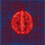
(b) Gold standard FBP

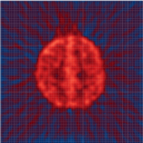
(c) GCV-reconstructed FBP

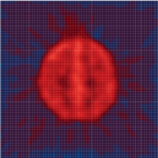
(d) MRUP-reconstructed FBP

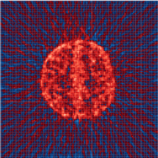
(e) MRUE-reconstructed FBP

Figure 1: (a) The phantom, with colormap (ranging from [-1,1] to account for negative artifacts) that is used for all the reconstructed images in this article. BPF reconstruction using the (b) optimal, (c) GCV- (d) MRUE- and (e) MRUP-selected bandwidths.

Pseudo-random Poisson realizations were simulated in the sinogram domain with mean intensity given by the corresponding discretized Radon transform of the phantom. The total expected counts $\Lambda$ varied over 9 distinct equi-spaced (on a $\log_{2}$ scale) values between $10^{4}$ and $10^{6}$ counts. Therefore, $\Lambda$ ranged from the very low (about 0.61 counts per pixel) to the moderately high (61 counts per pixel) and matched the range of values typically seen in individual scans in dynamic 2D PET studies [58]. Our first set of evaluations used a radially symmetric Gaussian kernel $\boldsymbol{S}_{h}$ with FWHM $h$. Subsequent evaluations used elliptically symmetric Gaussian kernels with parameters $h_{1},h_{2},\rho$. We use “BPFe” to denote BPF reconstructions with elliptically symmetric kernels and “GCVe” to denote GCV estimated parameters in these settings. We also evaluated performance in applying reducing negative artifacts as per [28] – we add “+” in the nomenclature to denote this additional postprocessing step. For each simulated sinogram dataset, we obtained the optimal BPF, BPFe, BPF+ and BPFe+ reconstructions and the corresponding optimal bandwidths as follows: for the BPF reconstruction $\hat{\boldsymbol{\lambda}}^{h}$ using a radially symmetric Gaussian filter with FWHM $h$, we calculated the Root Mean Squared Error (RMSE) $\mathcal{R}_{h}=\parallel\!\hat{\boldsymbol{\lambda}}^{h}-\boldsymbol{\lambda}\!\parallel/\sqrt{p}$, with $\boldsymbol{\lambda}$ the true source distribution (the Hoffman [57] phantom). The $h_{O}$ corresponding to the BPF reconstruction that minimizes the RMSE (i.e., the $h_{O}$ such that $\mathcal{R}_{h_{O}}\leq\mathcal{R}_{h}$ for all $h\neq h_{O}$) is our true optimal FWHM for the simulated sinogram dataset. Similar optimal FWHM parameters and gold standard reconstructions were obtained for BPFe, BPF+ and BPFe+ reconstructions (note that BPFe and BPFe+ have trivariate smoothing parameters.) We evaluated performance of reconstructions obtained using our GCV-estimated procedure ($h_{G}$) in terms of the RMSE and compared them (for BPF and BPF+ reconstructions) with corresponding calculations obtained using the MRUE- and MRUP-estimated [39, 40] bandwidths $h_{E}$ and $h_{P}E$, respectively. We also evaluated performance of each reconstruction in terms of its RMSE efficiency relative to the gold standard reconstruction obtained using $h_{O}$, that is, we calculated RMSE efficiency for a BPF reconstruction with filter resolution $h$ as $\mathcal{R}_{h}/\mathcal{R}_{h_{O}}$. Corresponding evaluations were done for BPFe, BPF+ and BPFe+ reconstructions, with smoothing parameters in BPFe and BPFe+ optimized over trivariate sets. Reducing negativity artifacts does not involve choosing a $h$ beyond that chosen for BPF or BPFe; however the optimal BPF+ or BPFe+ bandwidths may be different from the optimal BPF and BPFe ones. We simulated 1000 sinogram datasets and evaluated reconstruction performance using the different methods.

III-B Results

III-B1 Illustrative Examples

We first illustrate performance on a sample simulated sinogram realization with $\Lambda=10^{5}$.

BPF reconstruction

Figure 1b provides the “gold standard” BPF/FBP reconstruction

TABLE I: Bandwidths and RMSEs obtained with BPF reconstructions using bandwidths from different selection methods.

Estimation Method	Gold Standard	GCV	MRUP	MRUE
Optimal Bandwidth	3.183	3.279	15.32	1.397
RMSE ($\times 10^{-5}$)	$8.376$	$8.378$	$10.32$	$10.83$

obtained using $h_{O}$. BPF reconstructions obtained using $h_{G}$, $h_{P}$ and $h_{E}$ are in Figures 1c, 1d and 1e, respectively. Table I provides the estimated bandwidths and numerically summarizes performance in terms of the RMSEs. Performance using MRUE ($h_{E}=1.397$ pixels, RMSE$=1.083\times 10^{-4}$) and MRUP ($h_{P}=15.322$ pixels, RMSE$=1.032\times 10^{-4}$) bandwidths is not satisfactory, with the methods considerably under- and over-estimating the bandwidths, respectively. (Following [39], $h_{P}$ is specified in the 1D filtering domain of the projection distances, and is not directly comparable in numerical value to the 2D filter bandwidth). On the other hand, GCV ($h_{G}=3.279$ pixels, RMSE $=8.378\times 10^{-5}$) tracks the optimal value ($h_{O}=3.183$ pixels, RMSE $=8.376\times 10^{-5}$) very closely, both in terms of bandwidth selection and reconstruction ability.

BPFe reconstruction

We next illustrate GCVe’s performance in choosing optimal parameters for BPFe reconstructions. Figure 2 shows reconstructions obtained using the

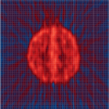
(a) BPFe Gold standard

(b) GCVe reconstruction

Estimation Method Optimal Parameters RMSE $(h_{1},h_{2},\rho)$ ($\times 10^{-5}$) Gold Standard (5.143, 2.488, -0.122) 8.289 GCVe-estimated (3.249, 3.058, 0.170) $8.378$

(c) Reconstruction performance

Figure 2: BPFe reconstructions with the (a) optimal and (b) GCVe-estimated smoothing parameters along with (c) summary of reconstruction performance.

true optimal and the GCVe-selected parameters. The

(a) BPF+ Gold standard

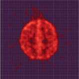
(b) GCV+

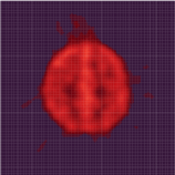
(c) MRUP+

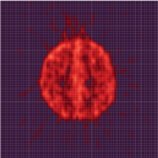
(d) BPFe+ Gold standard

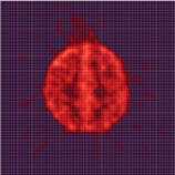
(e) GCVe+

Figure 3: (a-c) BPF+ reconstructions using the (a) optimal, (b) GCV- and (c) MRUP-estimated bandwidths. (d, e) BPFe+ reconstructions using the (d) optimal and (e) GCVe-estimated parameters.

reconstruction RMSE (Figure 2c) of $8.367\times 10^{-5}$ obtained using BPFe with GCVe even marginally outperforms BPF reconstruction using $h_{O}$ and compares favorably with the true optimal RMSE of $8.289\times 10^{-5}$. The illustration shows some undersmoothing with GCVe and scope for improved parameter estimates, but the wider class of elliptically symmetric kernels throws opens the possibility for further improvements to reconstruction.

Reconstructions with reduced negative artifacts

We also explored performance in BPF+ and BPFe+ reconstructions, having gold standards as per Figure 3a ($h_{O+}=2.766$; RMSE = $7.873\times 10^{-5}$) and Figure 3d ($h_{1}=3.818,h_{2}=2.216,\rho=-0.035$; RMSE = $7.831\times 10^{-5}$), respectively. For BPF+, the GCV-estimated bandwidth of $h=3.279$ yields the reconstruction of Figure 3b (RMSE$=7.976\times 10^{-5}$) while MRUP provides the BPF+ reconstruction of Figure 3c (RMSE=$1.008\times 10^{-4}$). For brevity of display, we forego discussing BPF+ reconstructions done with MRUE-selected bandwidths, noting simply that they also improve over BPF under BPF+ (with RMSE=$8.646\times 10^{-5}$ in this example) but that improvement falls far short of that obtained using GCV. Figure 3e also shows improvement of BPFe+ over BPFe (RMSE = $7.968\times 10^{-5}$) when negative artifacts are eliminated using [28], but the improvement is very marginal. Note that [28] reduces negative artifacts using a radially symmetric filter – an alternative approach that allows for greater flexibility in smoothing out negative values may be more appropriate.

III-B2 Large-scale Simulation Study

We report results of our large-scale simulation study on the performance (in terms of RMSE) of the different bandwidth selection and reconstruction methods and their distribution for different values of $\Lambda$. Reconstructions using MRU bandwidths have RMSEs substantially higher than those using the optimal or GCV-estimated bandwidths (Figure 4a) and certainly for lower values of $\Lambda$, so we display performance of these estimators separately in Figure 4b in order to attain finer granularity for displays involving our methods. Figure 4a displays RMSEs of BPF, BPFe, BPF+ and BPFe+ reconstructions obtained with GCV and the corresponding true optimal bandwidth parameters. The BPFe reconstructions using the GCVe-estimated bandwidths have similar, if not lower RMSEs, to those obtained with the gold standard BPF reconstructions. Reducing negative artifacts [28] improves the quality of BPF or BPFe reconstructions that is more substantial at higher $\Lambda$-values. But the improvement with using GCVe-estimated elliptically symmetric filters over GCV-estimated radially symmetric filters tapers off at higher total expected counts. However, the optimal BPFe estimator improves reconstruction quality in terms of having lower RMSEs over the gold standard BPF reconstructions. Thus, the performance of GCVe-estimated reconstruction relative to the gold standard BPFe is not as strong as that of the GCV-estimated reconstruction relative to the BPF gold standard. This observation is also supported by the relative RMSE efficiency displays in Figure 4c. This may be because, as per the table in Figure 2c of our illustrative example, the bandwidth parameter sets are quite different than the true optimal BPFe parameters.

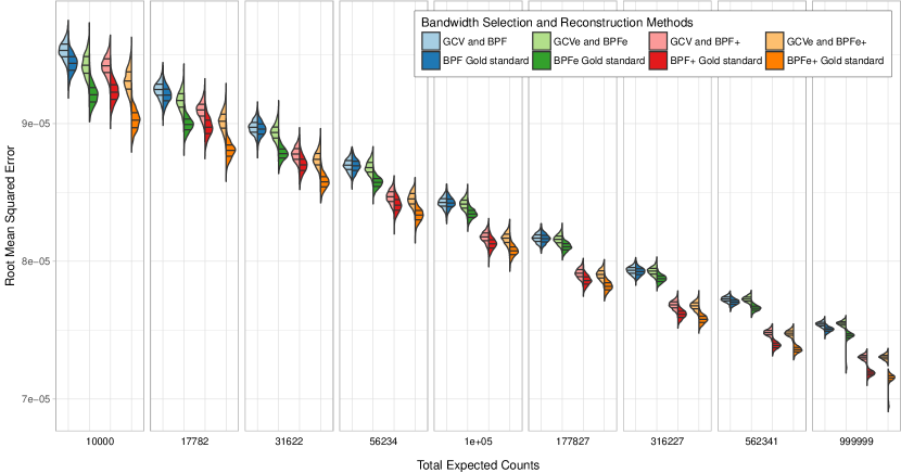
(a)

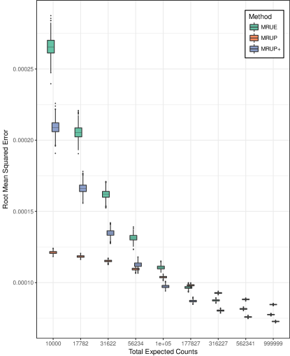
(b)

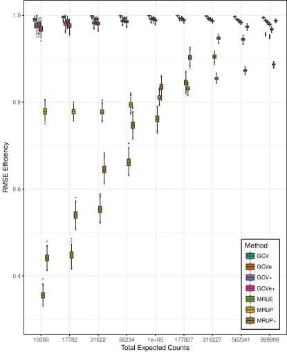
(c)

Figure 4: (a) Split violin plot distributions against total expected counts ($\Lambda$) of the 1000 RMSEs for reconstructions using GCV-estimated (left violin lobe) and the corresponding gold standard (right lobe) reconstruction. For each $\Lambda$-value, violins are in the order of BPF, BPFe, BPF+ and BPFe+ reconstructions. Bars on each split violin display the upper, median and lower quartiles of the RMSEs. (b)RMSEs of MRUE, MRUP and MRUP+ reconstructions and (c) RMSEs of all reconstructions relative to the corresponding gold standard for different total expected counts using different bandwidth selection and reconstruction methods.

Nevertheless, Figure 4a shows that any of the GCV methods out-performs the MRUE methods, especially at low total expected counts, both in terms of raw RMSE (Figure 4b) and relative RMSE efficiency (Figure 4c). Indeed, the relative RMSE efficiencies are almost always above 0.95 for the GCV methods. However, the MRU reconstructions are rather poor, especially at lower values of $\Lambda$. The MRUP results reported here are a bit more pessimistic than those over limited $\Lambda$ reported in [39] and [40]. Interestingly and contrary to their results, for larger (but not smaller) values of $\Lambda$, MRUE outperforms MRUP: comparison with their computer code indicates that the optimal bandwidths are often attained outside their chosen ranges for several cases. Reducing negative artifacts as per [28] improves MRUE reconstructions slightly – we omit these RMSEs in Figures 4b and 4c for clarity of display. The methods of [28] degrades MRUP reconstructions for lower $\Lambda$-values but with increasing $\Lambda$, MRUP+ generally performs the best among all MRUE estimates. The rate of efficiency of reconstructions with increasing $\Lambda$ obtained using GCV-selected bandwidths is lower than either MRUE or MRUP, but the implications are unclear, given its superior performance at all $\Lambda$. The results point to the ability of the GCV-estimated bandwidths in obtaining improved reconstructions in situations with low and high expected total emissions.

III-C Some Theoretical Analysis of the GCV Selector

We now discuss some theoretical properties of the reconstructions obtained using the GCV-selected bandwidth. Because our primary setting for investigating bandwidth selection in this article is PET and because of the additional complication provided by the Poisson distribution of the emissions, our investigation is in the context of an idealized emission tomography experiment. Suppose that we have $\boldsymbol{y}$ realized from an inhomogeneous Poisson Process with $\mathbb{E}(\boldsymbol{y})=\boldsymbol{\mu}=\boldsymbol{K}\boldsymbol{\lambda}$, and $\Lambda=\sum_{d,\theta}\mu_{d,\theta}$. Our interest is in estimating $\boldsymbol{f}=\boldsymbol{\lambda}/\Lambda$, for which we propose the estimator $\hat{\boldsymbol{f}}^{h}=\hat{\boldsymbol{\lambda}}^{h}/\hat{\Lambda}$. As in [40], define the loss function in the estimation and prediction domains to be $L_{e}(\hat{\boldsymbol{f}}^{h},\boldsymbol{f})=\parallel\!\hat{\boldsymbol{f}}^{h}-\boldsymbol{f}\!\parallel^{2}$ and $L_{P}(\hat{\boldsymbol{\mu}}^{h},\boldsymbol{\mu})=\Lambda^{-2}\parallel\!\hat{\boldsymbol{\mu}}^{h}-\boldsymbol{\mu}\!\parallel^{2}$, respectively, with corresponding risk functions as ${\mathcal{R}}_{e}(\hat{\boldsymbol{f}}^{h},\boldsymbol{f})$ and ${\mathcal{R}}_{P}(\hat{\boldsymbol{\mu}}^{h},\boldsymbol{\mu})$. From the SVD of $\boldsymbol{K}=\boldsymbol{U}_{1}\boldsymbol{D}_{\bullet}\boldsymbol{V}$ (where $\boldsymbol{U}_{1}^{\prime}\boldsymbol{U}_{1}=\boldsymbol{I}_{p}$ when $n\geq p$), we have $\boldsymbol{K}^{\prime}\boldsymbol{K}=\boldsymbol{V}\boldsymbol{D}^{2}_{\bullet}\boldsymbol{V}^{\prime}$, $(bK^{\prime}\boldsymbol{K})^{-1}=\boldsymbol{V}\boldsymbol{D}^{-2}_{\bullet}\boldsymbol{V}^{\prime}$. Also $\boldsymbol{S}_{h}=\boldsymbol{V}\boldsymbol{\Omega}_{h}\boldsymbol{V}^{\prime}$ because it is circulant, so that $\boldsymbol{S}_{h}(\boldsymbol{K}^{\prime}\boldsymbol{K})^{-1}\boldsymbol{K}^{\prime}=\boldsymbol{V}\boldsymbol{\Omega}_{h}\boldsymbol{D}_{\bullet}^{-1}\boldsymbol{U}_{1}^{\prime}$ and $\boldsymbol{K}\boldsymbol{S}_{h}(\boldsymbol{K}^{\prime}\boldsymbol{K})^{-1}\boldsymbol{K}^{\prime}=\boldsymbol{U}_{1}\boldsymbol{\Omega}_{h}\boldsymbol{U}_{1}^{\prime}$. Then

$$\begin{split}{\mathcal{R}}_{P}(\hat{\boldsymbol{\mu}}^{h},\boldsymbol{\mu})&=\Lambda^{-2}\mathbb{E}\parallel\!\boldsymbol{K}\boldsymbol{S}_{h}(\boldsymbol{K}^{\prime}\boldsymbol{K})^{-1}\boldsymbol{K}^{\prime}\boldsymbol{y}-\boldsymbol{K}\boldsymbol{\lambda}\!\parallel^{2}\\ &=\Lambda^{-2}\mathbb{E}\parallel\!\boldsymbol{U}_{1}\boldsymbol{\Omega}_{h}\boldsymbol{U}_{1}^{\prime}(\boldsymbol{y}-\boldsymbol{\mu})+\boldsymbol{K}\boldsymbol{S}_{h}\boldsymbol{\lambda}-\boldsymbol{K}\boldsymbol{\lambda}\!\parallel^{2}\\ &=\Lambda^{-2}\mathbb{E}\parallel\!\boldsymbol{U}_{1}\boldsymbol{\Omega}_{h}\boldsymbol{U}_{1}^{\prime}(\boldsymbol{y}-\boldsymbol{\mu})-\boldsymbol{U}_{1}\boldsymbol{D}_{\bullet}(\boldsymbol{I}_{p}-\boldsymbol{\Omega}_{h})\boldsymbol{V}^{\prime}\boldsymbol{\lambda}\!\parallel^{2}.\\ &=\Lambda^{-2}\mathbb{E}[tr\{(\boldsymbol{y}-\boldsymbol{\mu})^{\prime}\boldsymbol{U}_{1}\boldsymbol{\Omega}_{h}^{2}\boldsymbol{U}_{1}^{\prime}(\boldsymbol{y}-\boldsymbol{\mu})]\\ &\qquad\qquad+\Lambda^{-2}\mathbb{E}[tr\{(\boldsymbol{y}-\boldsymbol{\mu})^{\prime}\boldsymbol{U}_{1}\boldsymbol{\Omega}_{h}^{2}\boldsymbol{D}_{\bullet}(\boldsymbol{I}_{p}-\boldsymbol{\Omega}_{h})\boldsymbol{V}^{\prime}\boldsymbol{\lambda}\}]+\Lambda^{-2}tr\{\boldsymbol{\lambda}^{\prime}\boldsymbol{V}(\boldsymbol{I}_{p}-\boldsymbol{\Omega}_{h})^{2}\boldsymbol{D}_{\bullet}^{2}\boldsymbol{V}^{\prime}\boldsymbol{\lambda}\}.\\ \end{split}$$

Interchanging the expectation and the trace operators, the second term vanishes because $\mathbb{E}\boldsymbol{y}=\boldsymbol{\mu}$. Also using the property that the trace of the product of two conformable matrices is the trace of their product in the reverse order (as long as they are also conformable in the reverse order), the first term equals $\Lambda^{-2}tr[\boldsymbol{V}\boldsymbol{D}_{\bullet}^{-1}\boldsymbol{\Omega}_{h}\boldsymbol{U}_{1}^{\prime}\boldsymbol{U}_{1}\boldsymbol{\Omega}_{h}\boldsymbol{D}_{\bullet}^{-1}\boldsymbol{V}^{\prime}\boldsymbol{\Sigma}]$ and then

$${\mathcal{R}}_{P}(\hat{\boldsymbol{\mu}}^{h},\boldsymbol{\mu})=\Lambda^{-2}tr\{\boldsymbol{U}_{1}\boldsymbol{\Omega}_{h}^{2}\boldsymbol{U}_{1}^{\prime}\boldsymbol{\Sigma}+\boldsymbol{\lambda}^{\prime}\boldsymbol{V}\boldsymbol{D}_{\bullet}^{2}(\boldsymbol{I}_{p}-\boldsymbol{\Omega}_{h})^{2}\boldsymbol{V}^{\prime}\boldsymbol{\lambda}\}.$$

Under the idealized conditions of this section, $\boldsymbol{\Sigma}\equiv\mbox{diag}(\boldsymbol{\mu})$ is the dispersion matrix of $\boldsymbol{y}$. Now ${\mathcal{R}}_{e}(\hat{\boldsymbol{f}}^{h},\boldsymbol{f})=\Lambda^{-2}\mathbb{E}\parallel\!\hat{\boldsymbol{\lambda}}^{h}-\boldsymbol{\lambda}\!\parallel^{2}=\Lambda^{-2}\mathbb{E}\parallel\!\boldsymbol{V}\boldsymbol{\Omega}_{h}\boldsymbol{D}_{\bullet}^{-1}\boldsymbol{U}_{1}^{\prime}\boldsymbol{y}-\boldsymbol{\lambda}\!\parallel^{2}$ and using similar arguments as for ${\mathcal{R}}_{P}(\hat{\boldsymbol{\mu}}^{h},\boldsymbol{\mu})$ yields

$${\mathcal{R}}_{e}(\hat{\boldsymbol{f}}^{h},\boldsymbol{f})=\Lambda^{-2}tr\{\boldsymbol{U}_{1}\boldsymbol{D}_{\bullet}^{-2}\boldsymbol{\Omega}_{h}^{2}\boldsymbol{U}_{1}^{\prime}\boldsymbol{\Sigma}+\boldsymbol{\lambda}^{\prime}\boldsymbol{V}(\boldsymbol{I}_{p}-\boldsymbol{\Omega}_{h})^{2}\boldsymbol{V}^{\prime}\boldsymbol{\lambda}\}=\Lambda^{-2}tr\{\boldsymbol{D}_{\bullet}^{-2}[\boldsymbol{\Omega}_{h}^{2}\boldsymbol{U}_{1}^{\prime}\boldsymbol{\Sigma}\boldsymbol{U}_{1}+\boldsymbol{D}_{\bullet}^{2}(\boldsymbol{I}_{p}-\boldsymbol{\Omega}_{h})^{2}\boldsymbol{V}^{\prime}\boldsymbol{\lambda}\boldsymbol{\lambda}^{\prime}\boldsymbol{V}]\}.$$

Exploiting the diagonality of $\boldsymbol{D}_{\bullet}$ and the nonnegative definiteness of the matrices inside the trace operator yields that ${\mathcal{R}}^{\prime}_{e}(\hat{\boldsymbol{f}}^{h},\boldsymbol{f})\leq tr\{\boldsymbol{D}_{\bullet}^{-2}\}{\mathcal{R}}^{\prime}_{P}(\hat{\boldsymbol{\mu}}^{h},\boldsymbol{\mu})$. Using similar arguments, ${\mathcal{R}}^{\prime}_{P}(\hat{\boldsymbol{\mu}}^{h},\boldsymbol{\mu})\leq tr\{\boldsymbol{D}_{\bullet}^{2}\}{\mathcal{R}}^{\prime}_{e}(\hat{\boldsymbol{f}}^{h},\boldsymbol{f})$ so that both risks are minimized at the same $h$. From Theorem 1,

$$\begin{split}\Lambda^{-2}\mathbb{E}\zeta(h)&=\Lambda^{-2}\{tr[(\boldsymbol{I}_{p}-\boldsymbol{\Omega}_{h})^{2}\boldsymbol{U}_{1}^{\prime}\boldsymbol{\Sigma}\boldsymbol{U}_{1}]+\boldsymbol{\lambda}^{\prime}\boldsymbol{V}(\boldsymbol{I}_{p}-\boldsymbol{\Omega}_{h})^{2}\boldsymbol{D}_{\bullet}^{2}\boldsymbol{V}^{\prime}\boldsymbol{\lambda}+(1+c(h))^{2}tr\boldsymbol{U}_{2}^{\prime}\boldsymbol{\Sigma}\boldsymbol{U}_{2}\}\\ &={\mathcal{R}}_{P}(\hat{\boldsymbol{\mu}}^{h},\boldsymbol{\mu})+\Lambda^{-2}[\{1+c(h)\}^{2}tr\boldsymbol{\Sigma}-\{2c(h)+c^{2}(h)tr\boldsymbol{U}_{1}^{\prime}\boldsymbol{\Sigma}\boldsymbol{U}_{1}-2tr\boldsymbol{\Omega}_{h}\boldsymbol{U}_{1}^{\prime}\boldsymbol{\Sigma}\boldsymbol{U}_{1}\}]\\ &={\mathcal{R}}_{P}(\hat{\boldsymbol{\mu}}^{h},\boldsymbol{\mu})+\Lambda^{-1}[\{1+c(h)\}^{2}\vartheta_{n,p}-\{2c(h)+c^{2}(h)\}tr\boldsymbol{\varphi}_{n,p}-2tr\boldsymbol{\Omega}_{h}\boldsymbol{\varphi}_{n,p}],\end{split}$$

where $\vartheta_{n,p}=\Lambda^{-1}tr\boldsymbol{\Sigma}$ and the matrix $\boldsymbol{\varphi}_{n,p}=\Lambda^{-1}\boldsymbol{U}^{\prime}\boldsymbol{\Sigma}\boldsymbol{U}$ are both free of $\Lambda$. Thus, as $\Lambda\rightarrow\infty$,

$$\frac{\mid\mathbb{E}\zeta(h)-{\mathcal{R}}_{P}(\hat{\boldsymbol{\mu}}^{h},\boldsymbol{\mu})\mid}{{\mathcal{R}}_{P}(\hat{\boldsymbol{\mu}}^{h},\boldsymbol{\mu})}\rightarrow 0.$$

For $n>>p$, we have $\mathbb{E}\zeta^{\prime}(h)\approx{\mathcal{R}}^{\prime}_{P}(\hat{\boldsymbol{\mu}}^{h},\boldsymbol{\mu})-\frac{2}{\Lambda}\frac{d}{dh}tr\boldsymbol{\Omega}_{h}\boldsymbol{\varphi}_{n,p}$ so that for large $\Lambda$, the risk has an inflexion point close to the bandwidth optimizing $\mathbb{E}\zeta(h)$. On the other hand, for smaller values of $\Lambda$, the $h$ optimizing ${\mathcal{R}}_{P}(\hat{\boldsymbol{\mu}}^{h},\boldsymbol{\mu})$ is large and close to the minimizer for $\mathbb{E}\zeta(h)$. (To see this, consider the example of using a Butterworth filter for which the $\nu$th diagonal element of $\boldsymbol{\Omega}_{h}$ is $(1+h\parallel\nu\parallel^{r})^{-1}$.) This discussion provides some theoretical understanding of GCV’s good performance in selecting $h$ for all values of $\Lambda$ when $n>>p$ as is the case with emission tomography or in our experiments.

A reviewer wondered about performance when $n>>p$ is not satisfied. The supplement shows results on our large-scale simulation study done for cases when $\boldsymbol{K}^{\prime}\boldsymbol{K}$ is nearly ill-conditioned, and also not as well-conditioned as in our experiments in Section III-B2. Interestingly the GCV-estimated BPF methods do not do well relative to the optimal, but the GCV-estimated BPF+ methods continue to do well. This phenomenon needs more study.

IV Discussion

This paper developed a computationally efficient and practical approach to selecting the filter resolution size in 2D FBP reconstructions. Our approach hinges on implementing FBP through its equivalent BPF form, uses GCV and outperforms available adaptive methods in simulated PET studies, irrespective of the total expected rates of emissions. The approach also has the ability to incorporate a wider class of elliptically symmetric 2D reconstruction filters with the potential for further improving performance. In general, FBP is more commonly used than BPF, but this is perhaps because of its origins in X-ray computed tomography where reconstruction can begin along LORs for a given projection angle even while data along other projection angles are being acquired. However, in emission tomography, the data need to be completely acquired in the given time interval before reconstruction can begin so using BPF may not be much of a slower alternative to FBP. The easy estimation of the filter resolution size and its good performance even at lower emissions rates (which translates to lower signal-noise ratio for other applications) potentially makes it desirable to also use BPF in applications where reconstruction in the form of the 1D filtering step can be begun synchronous with data acquisition at other projection angles also, This would hold especially if the waiting time for data acquisition at all angles is more than compensated by the increased reconstruction accuracy afforded by GCV selection of the bandwidth. Methods speeding up backprojection [59] can further reduce the cost for using BPF.

There are a number of extensions that could benefit from our development. For instance, adopting an improved windowing function for windowed FBP has been shown [60] to improve reconstruction accuracy over FBP. It would be instructive to see the performance of GCV-selected bandwidths in such scenarios. Separately, the FORE algorithms [30] recast the 3D PET reconstruction problem into several 2D reconstructions. [61] showed that FORE reconstructions using ordered subsets expectation maximization (FORE+OSEM) are out-performed by the attenuation-weighted ordered subsets expectation maximization (FORE+AWOSEM) refinement and FORE+FBP reconstructions. It would be worth investigating whether FORE+FBP reconstructions can be further improved by using BPFe+ in place of FBP, and with optimal GCVe-estimated bandwidth. It would also be worth evaluating whether BPFe+ reconstructions with optimal GCVe-estimated bandwidths can improve estimates of kinetic model parameters in dynamic PET imaging where FBP reconstructions are the norm. There is scope for optimism here, given our method’s good performance for both lower and higher radiotracer uptake values. Nevertheless, this performance needs to be evaluated and calibrated in such contexts. Finally, another set of potential extensions could make possible the practical implementation of penalized reconstruction methods [50] in BPF or for regularizing reconstructions obtained using [22, 23, 27]. Thus, we see that while the methods developed here show promise in improving 2D FBP/BPF reconstruction by improved estimation of the filter resolution size using GCV, issues that merit further attention remain.

-A Proof of Theorem 1

The development and proof of the theorem closely mirror that of estimating the ridge regression parameter in [43]. Define the $(n-1)\times p$ matrix $\boldsymbol{K}_{-j}$ to be $\boldsymbol{K}$ with the $j$th row $\boldsymbol{k}_{j}^{\prime}$ removed. So, $\boldsymbol{K}^{\prime}=(\boldsymbol{K}_{-j}^{\prime},\boldsymbol{k}_{j})$. We will use the following equalities: $\boldsymbol{K}_{-j}^{\prime}\boldsymbol{K}_{-j}=\boldsymbol{K}^{\prime}\boldsymbol{K}-\boldsymbol{k}_{j}\boldsymbol{k}_{j}^{\prime}$ and $\boldsymbol{K}_{-j}\boldsymbol{y}_{-j}=\boldsymbol{K}\boldsymbol{y}-\boldsymbol{k}_{j}y_{j}$ and $\hat{\boldsymbol{\lambda}}_{-j}^{h}=\boldsymbol{S}_{h}(\boldsymbol{K}_{-j}^{\prime}\boldsymbol{K}_{-j})^{-1}\boldsymbol{K}_{-j}\boldsymbol{y}_{-j}$. The LOOCV mean squared error (CVMSE) is $\tau(h)=\frac{1}{n}\sum_{j=1}^{n}(\boldsymbol{k}_{j}^{\prime}\hat{\boldsymbol{\lambda}}^{h}_{-j}-y_{j})^{2}.$ Let $\hat{\boldsymbol{\lambda}}=\boldsymbol{Q}_{\boldsymbol{K}}\boldsymbol{K}^{\prime}\boldsymbol{y}$ be the (unsmoothed) LS reconstruction, with $\boldsymbol{Q}_{\boldsymbol{K}}\equiv(\boldsymbol{K}^{\prime}\boldsymbol{K})^{-1}$ in order to compress expressions. Using the Sherman-Morrison-Woodbury theorem, it follows that

$$\begin{split}\boldsymbol{k}_{j}^{\prime}\hat{\boldsymbol{\lambda}}^{h}_{-j}-y_{j}&=\boldsymbol{k}_{j}^{\prime}\boldsymbol{S}_{h}\left[\boldsymbol{Q}_{\boldsymbol{K}}+\frac{\boldsymbol{Q}_{\boldsymbol{K}}\boldsymbol{k}_{j}\boldsymbol{k}_{j}^{\prime}\boldsymbol{Q}_{\boldsymbol{K}}}{1-\boldsymbol{k}_{j}^{\prime}\boldsymbol{Q}_{\boldsymbol{K}}\boldsymbol{k}_{j}}\right](\boldsymbol{K}^{\prime}y-\boldsymbol{k}_{j}y_{j})-y_{j}\\ &=\boldsymbol{k}_{j}^{\prime}\hat{\boldsymbol{\lambda}}^{h}+\frac{\boldsymbol{k}_{j}^{\prime}\boldsymbol{S}_{h}\boldsymbol{Q}_{\boldsymbol{K}}\boldsymbol{k}_{j}\boldsymbol{k}_{j}^{\prime}\hat{\boldsymbol{\lambda}}}{1-\boldsymbol{k}_{j}^{\prime}\boldsymbol{Q}_{\boldsymbol{K}}\boldsymbol{k}_{j}}-\boldsymbol{k}_{j}^{\prime}\boldsymbol{S}_{h}\boldsymbol{Q}_{\boldsymbol{K}}\boldsymbol{k}_{j}y_{j}-\frac{\boldsymbol{k}_{j}^{\prime}\boldsymbol{S}_{h}\boldsymbol{Q}_{\boldsymbol{K}}\boldsymbol{k}_{j}\boldsymbol{k}_{j}^{\prime}\boldsymbol{Q}_{\boldsymbol{K}}\boldsymbol{k}_{j}y_{j}}{1-\boldsymbol{k}_{j}^{\prime}\boldsymbol{Q}_{\boldsymbol{K}}\boldsymbol{k}_{j}}-y_{j}\\ &=(\boldsymbol{k}_{j}^{\prime}\hat{\boldsymbol{\lambda}}^{h}-y_{j})+\frac{\Gamma_{jj,h}}{1-\Gamma_{jj}}(\boldsymbol{k}_{j}^{\prime}\hat{\boldsymbol{\lambda}}-y_{j})\\ \end{split}$$

where $\Gamma_{jj,h}=\boldsymbol{k}_{j}^{\prime}\boldsymbol{S}_{h}\boldsymbol{Q}_{\boldsymbol{K}}\boldsymbol{k}_{j}$ and $\Gamma_{jj}=\boldsymbol{k}_{j}^{\prime}\boldsymbol{Q}_{\boldsymbol{K}}\boldsymbol{k}_{j}$. Let $\boldsymbol{\Delta}_{h}$ be the diagonal matrix with $\Gamma_{jj,h}/(1-\Gamma_{jj})$ as the $(j,j)$th element. Then, using the above, the CVMSE reduces to

$$\begin{split}\tau(h)&=\frac{1}{n}\left\{\boldsymbol{y}^{\prime}\left[\boldsymbol{I}_{n}-\boldsymbol{K}\boldsymbol{S}_{h}\boldsymbol{Q}_{\boldsymbol{K}}\boldsymbol{K}^{\prime}\right]^{\prime}[\boldsymbol{I}_{n}-\boldsymbol{K}\boldsymbol{S}_{h}\boldsymbol{Q}_{\boldsymbol{K}}\boldsymbol{K}^{\prime}\right]\boldsymbol{y}+2\boldsymbol{y}^{\prime}\left[\boldsymbol{I}_{n}-\boldsymbol{K}\boldsymbol{S}_{h}\boldsymbol{Q}_{\boldsymbol{K}}\boldsymbol{K}^{\prime}\right]^{\prime}\boldsymbol{\Delta}_{h}\left[\boldsymbol{I}_{n}-\boldsymbol{K}\boldsymbol{Q}_{\boldsymbol{K}}\boldsymbol{K}^{\prime}\right]\boldsymbol{y}\\ &\qquad\qquad\left.+\boldsymbol{y}^{\prime}\left[\boldsymbol{I}_{n}-\boldsymbol{K}\boldsymbol{Q}_{\boldsymbol{K}}\boldsymbol{K}^{\prime}\right]^{\prime}\boldsymbol{\Delta}^{2}_{h}\left[\boldsymbol{I}_{n}-\boldsymbol{K}\boldsymbol{Q}_{\boldsymbol{K}}\boldsymbol{K}^{\prime}\right]\boldsymbol{y}\right\}.\end{split}$$ (6)

Let $\boldsymbol{D}_{\bullet}$ be the diagonal matrix of the square root of the $p$ eigenvalues of $\boldsymbol{K}^{\prime}\boldsymbol{K}$. Let $\boldsymbol{K}=\boldsymbol{U}\boldsymbol{D}\boldsymbol{V}^{\prime}$ be the SVD of $\boldsymbol{K}$ with $\boldsymbol{U}$ as in the theorem statement, $\boldsymbol{D}$ be $\boldsymbol{D}_{\bullet}$ augmented row-wise by an $(n-p)\times p$ matrix of zeros, and $\boldsymbol{V}$ have columns containing the right singular vectors of $\boldsymbol{K}$. Further, let $\boldsymbol{W}$ be the corresponding unitary matrix that diagonalizes any 1D (see [56]) or 2D (see Theorem 5) circulant matrix. Under the rotated generalized linear model having observations $\tilde{\boldsymbol{y}}=\boldsymbol{W}\boldsymbol{U}^{\prime}\boldsymbol{y}$, the reconstruction problem reformulates to estimating $\boldsymbol{\lambda}$ from $\mathbb{E}(\tilde{\boldsymbol{y}})=\boldsymbol{W}\boldsymbol{D}\boldsymbol{V}^{\prime}\boldsymbol{\lambda}\equiv\tilde{\boldsymbol{K}}\boldsymbol{\lambda}$, where $\tilde{\boldsymbol{K}}=\boldsymbol{W}\boldsymbol{D}\boldsymbol{V}^{\prime}$.

Now $\tilde{\boldsymbol{K}}^{\prime}\tilde{\boldsymbol{K}}=\boldsymbol{V}\boldsymbol{D}_{\bullet}^{2}\boldsymbol{V}^{\prime}$ so that $\tilde{\boldsymbol{K}}(\tilde{\boldsymbol{K}}^{\prime}\tilde{\boldsymbol{K}})^{-1}\tilde{\boldsymbol{K}}^{\prime}$ and $\tilde{\boldsymbol{K}}\boldsymbol{S}_{h}(\tilde{\boldsymbol{K}}^{\prime}\tilde{\boldsymbol{K}})^{-1}\tilde{\boldsymbol{K}}^{\prime}$ are both circulant, with each having exactly $p$ positive and non-zero eigenvalues given by the diagonal elements of $\boldsymbol{I}_{p}$ and $\boldsymbol{\Omega}_{h}$ respectively. Consequently $(\boldsymbol{I}_{n}-\tilde{\boldsymbol{K}}(\tilde{\boldsymbol{K}}^{\prime}\tilde{\boldsymbol{K}})^{-1}\tilde{\boldsymbol{K}}^{\prime})=\boldsymbol{W}{\mathcal{D}}_{(\boldsymbol{0}_{p},\boldsymbol{I}_{n-p})}\boldsymbol{W}^{*}$ and $(\boldsymbol{I}_{n}-\tilde{\boldsymbol{K}}\boldsymbol{S}_{h}(\tilde{\boldsymbol{K}}^{\prime}\tilde{\boldsymbol{K}})^{-1}\tilde{\boldsymbol{K}}^{\prime})=\boldsymbol{W}{\mathcal{D}}_{(\boldsymbol{I}_{p}-\boldsymbol{\Omega}_{h},\boldsymbol{I}_{n-p})}\boldsymbol{W}^{*}$ where $\boldsymbol{W}^{*}$ is the complex conjugate transpose of $\boldsymbol{W}$, $\boldsymbol{0}_{p}$ is a $p\times p$ matrix of zeros and ${\mathcal{D}}_{(\boldsymbol{A},\boldsymbol{B})}$ denotes a block-diagonal matrix with matrices $\boldsymbol{A}$ and $\boldsymbol{B}$ in the diagonals. Therefore, both $\tilde{\boldsymbol{K}}\boldsymbol{S}_{h}(\tilde{\boldsymbol{K}}^{\prime}\tilde{\boldsymbol{K}})^{-1}\tilde{\boldsymbol{K}}^{\prime}$ and $(\boldsymbol{I}-\tilde{\boldsymbol{K}}(\tilde{\boldsymbol{K}}^{\prime}\tilde{\boldsymbol{K}})^{-1}\tilde{\boldsymbol{K}}^{\prime})$ are circulant (the latter is also idempotent) with constant diagonals. In the rotated framework, $\Gamma_{jj,h}=tr(\boldsymbol{\Omega}_{h})/n$ (note that $tr(\boldsymbol{\Omega}_{h})$ is $p$ times any diagonal element of $\boldsymbol{S}_{h}$) while $1-\Gamma_{jj}=(n-p)/n$, and so $\boldsymbol{\Delta}_{h}=c(h)\boldsymbol{I}_{n}$. In the rotated framework, we consider the three terms in (6) individually. The first term reduces to

$$\tilde{\boldsymbol{y}}^{\prime}[\boldsymbol{I}-\tilde{\boldsymbol{K}}\boldsymbol{S}_{h}(\tilde{\boldsymbol{K}}^{\prime}\tilde{\boldsymbol{K}})^{-1}\tilde{\boldsymbol{K}}^{\prime}]^{\prime}[\boldsymbol{I}-\tilde{\boldsymbol{K}}\boldsymbol{S}_{h}(\tilde{\boldsymbol{K}}^{\prime}\tilde{\boldsymbol{K}})^{-1}\tilde{\boldsymbol{K}}^{\prime}]\tilde{\boldsymbol{y}}\equiv\boldsymbol{y}^{\prime}\boldsymbol{U}{\mathcal{D}}^{2}_{(\boldsymbol{I}_{p}-\boldsymbol{\Omega}_{h},\boldsymbol{I}_{n-p})}\boldsymbol{U}^{\prime}\boldsymbol{y}=\boldsymbol{z}_{1}^{\prime}(\boldsymbol{I}_{p}-\boldsymbol{\Omega}_{h})^{2}\boldsymbol{z}_{1}+\boldsymbol{z}_{2}^{\prime}\boldsymbol{z}_{2},$$

while the second term

$$2\tilde{\boldsymbol{y}}^{\prime}[\boldsymbol{I}_{n}-\tilde{\boldsymbol{K}}\boldsymbol{S}_{h}(\tilde{\boldsymbol{K}}^{\prime}\tilde{\boldsymbol{K}})^{-1}\tilde{\boldsymbol{K}}^{\prime}]^{\prime}\boldsymbol{\Delta}_{h}[\boldsymbol{I}_{n}-\tilde{\boldsymbol{K}}(\tilde{\boldsymbol{K}}^{\prime}\tilde{\boldsymbol{K}})^{-1}\tilde{\boldsymbol{K}}^{\prime}]\tilde{\boldsymbol{y}}\equiv 2c(h)\boldsymbol{y}^{\prime}\boldsymbol{U}{\mathcal{D}}_{(\boldsymbol{I}_{p}-\boldsymbol{\Omega}_{h},\boldsymbol{I}_{n-p})}{\mathcal{D}}_{(\boldsymbol{0}_{p,p},\boldsymbol{I}_{n-p})}\boldsymbol{U}\boldsymbol{y}=2c(h)\boldsymbol{z}_{2}^{\prime}\boldsymbol{z}_{2}$$

with $\boldsymbol{0}_{r,s}$ being the $r\times s$ matrix of zeroes. The third term

$$\tilde{\boldsymbol{y}}^{\prime}[\boldsymbol{I}_{n}-\tilde{\boldsymbol{K}}(\tilde{\boldsymbol{K}}^{\prime}\tilde{\boldsymbol{K}})^{-1}\tilde{\boldsymbol{K}}^{\prime}]^{\prime}\boldsymbol{\Delta}_{h}^{2}[\boldsymbol{I}_{n}-\tilde{\boldsymbol{K}}(\tilde{\boldsymbol{K}}^{\prime}\tilde{\boldsymbol{K}})^{-1}\tilde{\boldsymbol{K}}^{\prime}]\tilde{\boldsymbol{y}}\equiv c^{2}(h)\boldsymbol{y}^{\prime}\boldsymbol{U}{\mathcal{D}}_{(\boldsymbol{0}_{p},\boldsymbol{I}_{n-p})}\boldsymbol{U}^{\prime}\boldsymbol{y}=c^{2}(h)\boldsymbol{z}_{2}^{\prime}\boldsymbol{z}_{2}.$$

Theorem 1 follows, after scaling all sides by $n$. $\Box$

-B Proof of Theorem 2

Let $\ell$ be the integer part of $(p+1)/2$. Let $\boldsymbol{c}=\{c_{0},c_{1},c_{2},\ldots,c_{\ell-1},c_{\ell},c_{\ell-1},\ldots,c_{2},c_{1}\}$ be the first row of $\boldsymbol{\mathcal{C}}$ for even $p$; the middle term $c_{\ell}$ is absent for odd $p$. Writing the $k$th of the $p$ complex roots of unity as $\exp\{i2\pi k/p\}=\cos(2\pi k/p)+i\sin(2\pi k/p)$, the $k$th eigenvalue of $\boldsymbol{\mathcal{C}}$ is $d_{k}=\sum_{j=0}^{p-1}c_{j}\omega_{k}^{j}=c_{0}+\sum_{j=1}^{\ell-1}c_{j}\cos({2\pi kj}/p)+c_{p/2}(-1)^{\ell};0\leq k\leq p-1$, with the last term in the summation absent for $p$ odd. From [56] or directly, an eigenvector corresponding to $d_{k}$ is $\boldsymbol{\gamma}(\omega_{k})=\{1,\omega_{k}^{1},\omega_{k}^{2},\ldots,\omega_{k}^{p-1}\}$. Further, $d_{k}=d_{p-k}$ for $k=1,2\ldots,\ell-1$. This means that any symmetric circulant matrix has two (only one for $p$ odd) real eigenvalues of algebraic multiplicity one with eigenvectors given, up to constant division, by $\boldsymbol{1}=\{1,1,\ldots,1\}$ and (for $p$ even) $\pm\boldsymbol{1}=\{1,-1,1,-1,\ldots,1,-1\}$. There are at most $\ell-1$ distinct eigenvalues of algebraic multiplicity 2: for $1\leq k\leq\ell-1$, the eigenvectors corresponding to $d_{k}$ are $\gamma(\omega_{k})$ and $\gamma(\bar{\omega}_{k})$, where $\bar{\omega}_{k}$ is the complex conjugate of $\omega_{k}$. Therefore, $\gamma(\omega_{k})+\gamma(\bar{\omega}_{k})$ and $i(\gamma(\omega_{k})-\gamma(\bar{\omega}_{k}))$ are also distinct (and real) eigenvectors that correspond to $d_{k}$. Theorem 2 follows. $\Box$

Supplement

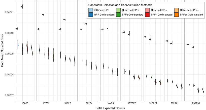
(a)

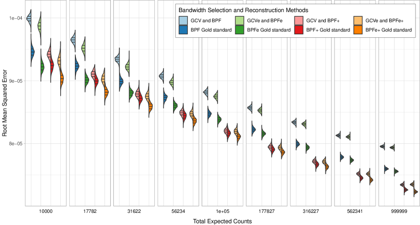
(b)

Figure S-1: Split violin plot distributions against total expected counts ($\Lambda$) of the 1000 RMSEs for reconstructions using GCV-estimated (left violin lobe) and the corresponding gold standard (right lobe) reconstructions for simulation experiments with (a) $128\times 129$ and (b) $128\times 160$ distance-angle pairs. The imaging domain had $128\times 128$ pixels.

References

- [1] R. N. Bracewell and A. C. Riddle, “Inversion of Fan-Beam Scans in Radio Astronomy,” The Astrophysical Journal, vol. 150, p. 427, Nov. 1967.
- [2] G. N. Ramachandran and A. V. Lakshminarayanan, “Three-dimensional reconstruction from radiographs and electron micrographs: Application of convolutions instead of fourier transforms,” Proceedings of the National Academy of Sciences, vol. 68, no. 9, pp. 2236–2240, 1971. [Online]. Available: http://www.pnas.org/content/68/9/2236
- [3] A. Kak and M. Slaney, Principles of Computerized Tomographic Imaging. IEEE Press, 1988.
- [4] R. M. Mersereau and A. V. Oppenheim, “Digital reconstruction of multidimensional signals from their projections,” Proceedings of the IEEE, vol. 62, no. 10, pp. 1319–1338, Oct 1974.
- [5] P. P. Bruyant, “Analytic and iterative reconstruction algorithms in spect,” Journal of Nuclear Medicine, vol. 43, no. 10, pp. 1343–1358, 2002.
- [6] G. T. Herman, Fundamentals of computerized tomography: Image reconstruction from projection, 2nd ed. Springer, 2009.
- [7] H. R. Na and H. Lee, “Resolution degradation parameters of ionospheric tomography,” Radio Science, vol. 29, no. 1, pp. 115–125, Jan.-Feb. 1994. [Online]. Available: https://agupubs.onlinelibrary.wiley.com/doi/abs/10.1029/93RS02734
- [8] J.-L. Starck and F. Murtagh, Astronomical image and data analysis, 2nd ed., ser. Astronomy and Astrophysics library. Berlin: Springer, 2006.
- [9] A. Haefner, D. Gunter, R. Barnowski, and K. Vetter, “A filtered back-projection algorithm for compton camera data,” IEEE Transactions on Nuclear Science, vol. 62, no. 4, pp. 1911–1917, Aug 2015.
- [10] Y. Nagata, J. Huang, J. D. Achenbach, and S. Krishnaswamy, “Lamb wave tomography using laser-based ultrasonics,” in Review of Progress in Quantitative Nondestructive Evaluation: Volume 14, D. O. Thompson and D. E. Chimenti, Eds. Boston, MA: Springer US, 1995, pp. 561–568. [Online]. Available: https://doi.org/10.1007/978-1-4615-1987-4˙68
- [11] W. Wright, D. Hutchins, D. Jansen, and D. Schindel, “Air-coupled lamb wave tomography,” IEEE Transactions on Ultrasonics, Ferroelectrics, and Frequency Control, vol. 44, no. 1, pp. 53–59, Jan 1997.
- [12] S. Lade, D. Paganin, and M. Morgan, “3-d vector tomography of doppler-transformed fields by filtered-backprojection,” Optics Communications, vol. 253, no. 4, pp. 382 – 391, 2005. [Online]. Available: http://www.sciencedirect.com/science/article/pii/S0030401805004189
- [13] X. Zhao, R. L. Royer, S. E. Owens, and J. L. Rose, “Ultrasonic lamb wave tomography in structural health monitoring,” Smart Materials and Structures, vol. 20, no. 10, p. 105002, 2011. [Online]. Available: http://stacks.iop.org/0964-1726/20/i=10/a=105002
- [14] A. Myagotin, A. Voropaev, L. Helfen, D. Hänschke, and T. Baumbach, “Efficient volume reconstruction for parallel-beam computed laminography by filtered backprojection on multi-core clusters,” IEEE Transactions on Image Processing, vol. 22, no. 12, pp. 5348–5361, Dec 2013.
- [15] K. Prabhat, K. A. Mohan, C. Phatak, C. Bouman, and M. D. Graef, “3d reconstruction of the magnetic vector potential using model based iterative reconstruction,” Ultramicroscopy, vol. 182, pp. 131 – 144, 2017. [Online]. Available: http://www.sciencedirect.com/science/article/pii/S0304399117301948
- [16] I. Sechopoulos, “A review of breast tomosynthesis. part ii. image reconstruction, processing and analysis, and advanced applications,” Medical Physics, vol. 40, no. 1, p. 014302, Jan 2013. [Online]. Available: https://aapm.onlinelibrary.wiley.com/doi/abs/10.1118/1.4770281
- [17] N. Megherbi, T. P. Breckon, G. T. Flitton, and A. Mouton, “Radon transform based automatic metal artefacts generation for 3d threat image projection,” pp. 8901 – 8901 – 9, 2013. [Online]. Available: https://doi.org/10.1117/12.2028506
- [18] M. Ter-Porgossian, M. E. Raichle, and B. E. Sobel, “Positron emission tomography,” Scientific American, vol. 243(4), pp. 170–181, 1980.
- [19] D. Hawe, F. R. H. Fernández, L. O’Suilleabháin, J. Huang, E. Wolsztynski, and F. O’Sullivan, “Kinetic analysis of dynamic positron emission tomography data using open-source image processing and statistical inference tools,” in Wiley Interdisciplinary Reviews: Computational Statistics, 2012, vol. 4, no. 3, pp. 316–322.
- [20] F. O’Sullivan, “Locally constrained mixture representation of dynamic imaging data from PET and MR studies,” Biostatistics, vol. 7:2, pp. 318–338, 2006.
- [21] E. Wolsztynski, F. O’Sullivan, J. O’Sullivan, and J. F. Eary, “Statistical assessment of treatment response in a cancer patient based on pre-therapy and post-therapy FDG-PET scans,” Statistics in Medicine, vol. 36, no. 7, pp. 1172–1200, 2017.
- [22] Y. Vardi, L. A. Shepp, and L. A. Kaufman, “Statistical model for positron emission tomography,” Journal of the American Statistical Association, vol. 80, pp. 8–37, 1985.
- [23] P. J. Green, “Bayesian reconstruction from positron emission tomography using a modified EM algorithm,” IEEE Transactions on Medical Imaging, vol. 9, pp. 84–93, 1990.
- [24] H. M. Hudson and R. S. Larkin, “Accelerated image reconstruction using ordered subsets of projection data,” IEEE Transactions on Medical Imaging, vol. 13, no. 4, pp. 601–609, Dec 1994.
- [25] J. Nuyts and J. A. Fessler, “A penalized-likelihood image reconstruction method for emission tomography, compared to postsmoothed maximum-likelihood with matched spatial resolution,” IEEE Transactions on Medical Imaging, vol. 22, no. 9, p. 1042–1052, 2003.
- [26] J. W. Stayman and J. A. Fessler, “Compensation for nonuniform resolution using penalized-likelihood reconstruction in space-variant imaging systems,” IEEE Transactions on Medical Imaging, vol. 23, no. 3, p. 269–284, 2004.
- [27] F. O’Sullivan and L. O’Suilleabháin, “A multi-grid approach to ML reconstruction in PET: A fast alternative to EM-based techniques,” in 2013 IEEE Nuclear Science Symposium and Medical Imaging Conference Record, 2013, pp. 1–5.
- [28] F. O’Sullivan, Y. Pawitan, and D. Haynor, “Reducing negativity artifacts in emission tomography: Post-processing filtered backprojection solutions,” IEEE Transactions on Medical Imaging, vol. 12, pp. 653–663, 1993.
- [29] F. O’Sullivan, “A study of least squares and maximum likelihood for image reconstruction in positron emission tomography,” Annals of Statistics, vol. 23:4, pp. 1267–1300, 1995.
- [30] M. Defrise, P. E. Kinahan, D. W. Townsend, C. Michel, M. Sibomana, and D. F. Newport, “Exact and approximate rebinning algorithms for 3-d PET data,” IEEE Transactions on Medical Imaging, vol. 16, no. 2, pp. 145–158, April 1997.
- [31] M. E. Daube-Witherspoon, L. M. Popescu, S. Matej, C. A. Cardi, R. M. Lewitt, and J. S. Karp, “Rebinning and reconstruction of point source transmission data for positron emission tomography,” in 2003 IEEE Nuclear Science Symposium. Conference Record (IEEE Cat. No.03CH37515), vol. 4, Oct 2003, pp. 2839–2843 Vol.4.
- [32] K. Lee, P. E. Kinahan, J. A. Fessler, R. S. Miyaoka, M. Janes, and T. K. Lewellen, “Pragmatic fully 3d image reconstruction for the mices mouse imaging pet scanner,” Physics in Medicine & Biology, vol. 49, no. 19, p. 4563, 2004. [Online]. Available: http://stacks.iop.org/0031-9155/49/i=19/a=008
- [33] P. Hall, “On global properties of variable bandwidth density estimators,” Annals of Statistics, vol. 20, pp. 762–778, 1992.
- [34] D. Nychka and D. D. Cox, “Convergence rates for regularized solutions of integral equations from discrete noisy data,” Annals of Statistics, vol. 17, pp. 556–572, 1989.
- [35] B. W. Silverman, Density Estimation for Statistics and Data Analysis. London: Chapman and Hall, 1986.
- [36] C. J. Stone, “An asymptotically optimal window selection rule for kernel density estimates,” Annals of Statistics, vol. 12, pp. 1289–1297, 1984.
- [37] G. Wahba, Spline Models in Statistics. Philadelphia: SIAM, 1990.
- [38] D. A. Girard, “Optimal regularized reconstruction in computer tomography,” SIAM Journal of Scientific and Statistical Computation, vol. 8, pp. 934–950, 1987.
- [39] Y. Pawitan and F. O’Sullivan, “Data-dependent bandwidth selection for emission computed tomography reconstruction,” IEEE Transactions on Medical Imaging, vol. 12, pp. 653–663, 1993.
- [40] F. O’Sullivan and Y. Pawitan, “Bandwidth selection for indirect density estimation based on corrupted histogram data,” Jounal of the American Statistical Association, vol. 91, pp. 610–627, 1996.
- [41] S. Geisser, “The predictive sample reuse method with applications,” Journal of the Americal Statistical Association, vol. 70(350), pp. 320–328, 1975.
- [42] C. J. Stone, “Cross-validation and multinomial prediction,” Biometrika, vol. 61, pp. 509–515, 1974.
- [43] G. H. Golub, M. Heath, and G. Wahba, “Generalized crossvalidation as a method for choosing a good ridge parameter,” Technometrics, vol. 21, pp. 215–223, 1979.
- [44] P. Craven and G. Wahba, “Smoothing noisy data with spline functions,” Numerical Methods, vol. 31, pp. 377–403, 1979.
- [45] S. J. Reeves and R. M. Merserau, “Optimal estimation of the regularization parameter and stabilizing functional for regularized image restoration,” Optical Engineering, vol. 29(5), pp. 445–454, 1990.
- [46] S. J. Reeves, “A cross-validation framework for solving image restoration problems,” Journal of Visual Communications and Image Representation, vol. 3, pp. 433–445, 1992.
- [47] N. Nguyen, P. Milanfar, and G. Golub, “Efficient generalized cross-validation with applications to parametric image restoration and resolution enhancement,” IEEE Transactions on Image Processing, vol. 10(9), pp. 1299–1308, 2001.
- [48] P. Hall and D. M. Titterington, “Common structure of techniques for choosing smoothing parameters in regression problems,” Journal of the Royal Statistical Society, B, vol. 49, pp. 184–198, 1987.
- [49] A. M. Thompson, J. C. Brown, J. W. Kay, and D. M. Titterington, “A study of methods of choosing the smoothing parameter in image restoration by regularization,” IEEE Transactions on Pattern Analysis and Machine Intelligence, vol. 13(4), pp. 326–339, 1991.
- [50] A. M. Thompson, J. W. Kay, and D. M. Titterington, “A cautionary note about crossvalidatory choice,” Journal of Statistical Computing and Simulation, vol. 33, pp. 199–216, 1989.
- [51] R. M. Mersereau and A. V. Oppenheim, “Digital reconstruction of multidimensional signals from their projections,” Proceedings of the IEEE, vol. 62, no. 10, pp. 1319–1338, October 1974.
- [52] F. Natterer, Mathematics of Computerized Tomography. New York: Wiley, 1986.
- [53] S. R. Deans, The Radon Transform and Some of Its Applications. Malabar, Florida: Krieger Publishing Company, 1993.
- [54] M. Wand and M. Jones, Kernel Smoothing. London: Chapman and Hall, 1995.
- [55] J. W. Demmel, Applied Numerical Linear Algebra. Philadelphia: SIAM, 1997.
- [56] R. Bellman, An Introduction to Matrix Analysis. New York: McGraw-Hill, 1960.
- [57] E. J. Hoffman, P. D. Cutler, W. M. Digby, and J. C. Mazziotta, “3-d phantom to simulate cerebral blood flow and metabolic images for pet,” IEEE Transactions on Nuclear Science, vol. 37, pp. 616–620, 1990.
- [58] M. E. Phelps, S. C. Huang, E. J. Hoffman, C. Selin, L. Sokoloff, and D. E. Kuhl, “Tomographic measurement of local cerebral glucose metabolic rate in humans with [f-18]2-fluoro-2-deoxy-d-glucose: Validation of method,” Annals of Neurology, vol. 6, pp. 371–388, 1979.
- [59] E. Miqueles, N. Koshev, and E. S. Helou, “A backprojection slice theorem for tomographic reconstruction,” IEEE Transactions on Image Processing, vol. 27, no. 2, pp. 894–906, Feb 2018.
- [60] G. L. Zeng, “Revisit of the ramp filter,” IEEE Transactions on Nuclear Science, vol. 62, no. 1, pp. 131–136, Feb 2015.
- [61] C. Lartizien, P. E. Kinahan, R. Swensson, C. Comtat, M. Lin, V. Villemagne, and R. Trébossen, “Evaluating image reconstruction methods for tumor detection in 3-dimensional whole-body pet oncology imaging,” Journal of Nuclear Medicine, vol. 44, no. 2, pp. 276–290, 2003. [Online]. Available: http://jnm.snmjournals.org/content/44/2/276.abstract