Error Estimation for Randomized Least-Squares Algorithms via the Bootstrap

Abstract

Over the course of the past decade, a variety of randomized algorithms have been proposed for computing approximate least-squares (LS) solutions in large-scale settings. A longstanding practical issue is that, for any given input, the user rarely knows the actual error of an approximate solution (relative to the exact solution). Consequently, the user often appeals to worst-case error bounds that tend to offer only qualitative guidance. As a more practical alternative, we propose a bootstrap method to compute a posteriori error estimates for randomized LS algorithms. These estimates permit the user to numerically assess the error of a given solution, and to predict how much work is needed to improve a “preliminary” solution. From a practical standpoint, the method also has considerable flexibility, insofar as it can be applied to several popular sketching algorithms, as well as a variety of error metrics. Moreover, the extra step of error estimation does not add much cost to an underlying sketching algorithm. Finally, we demonstrate the effectiveness of the method with both theoretical and empirical results.

Keywords: Bootstrap, matrix sketching, randomized linear algebra, least squares.

1 Introduction

Randomized sketching algorithms have been intensively studied in recent years as a general approach to computing fast approximate solutions to large-scale least-squares (LS) problems (Drineas et al., 2006, Rokhlin and Tygert, 2008, Avron et al., 2010, Drineas et al., 2011, Mahoney, 2011, Drineas et al., 2012, Clarkson and Woodruff, 2013, Woodruff, 2014, Ma et al., 2014, Meng et al., 2014, Pilanci and Wainwright, 2015, 2016). During this time, much progress has been made in analyzing the performance of these algorithms, and existing theory provides a good qualitative description of approximation error (relative to the exact solution) in terms of various problem parameters. However, in practice, the user rarely knows the actual error of a randomized solution, or how much extra computation may be needed to achieve a desired level of accuracy.

A basic source of this problem is that it is difficult to translate theoretical error bounds into numerical error bounds that are tight enough to be quantitatively meaningful. For instance, theoretical bounds are often formulated to hold for the worst-case input among a large class of possible inputs. Consequently, they are often pessimistic for “generic” problems, and they may not account for the structure that is unique to the input at hand. Another practical issue is that these bounds typically involve constants that are either conservative, unspecified, or dependent on unknown parameters.

In contrast with worst-case error bounds, we are interested in “a posteriori” error estimates. By this, we mean error bounds that can be estimated numerically in terms of the computed solution or other observable information. Although methods for obtaining a posteriori error estimates are well-developed in some areas of computer science and applied mathematics, there has been very little development for randomized sketching algorithms (cf. Section 1.4). (For brevity, we will usually omit the qualifier ‘a posteriori’ from now on when referring to error estimation.)

The main purpose of this paper is to show that it is possible to directly estimate the error of randomized LS solutions in a way that is both practical and theoretically justified. Accordingly, we propose a flexible estimation method that can enhance existing sketching algorithms in a variety of ways. In particular, we will explain how error estimation can help the user to (1) select the “sketch size” parameter, (2) assess the convergence of iterative sketching algorithms, and (3) measure error in a wider range of metrics than can be handled by existing theory.

1.1 Setup and Background

Consider a large, overdetermined LS problem, involving a rank $d$ matrix $A\in{\mathbb{R}}^{n\times d}$, and a vector $b\in{\mathbb{R}}^{n}$, where $n\gg d$. These inputs are viewed as deterministic, and the exact solution is denoted

$$x_{\textup{opt}}:=\mathop{\rm argmin}_{x\in{\mathbb{R}}^{d}}\|Ax-b\|_{2}.$$ (1)

The large number of rows $n$ is often a major computational bottleneck, and sketching algorithms overcome this obstacle by effectively solving a smaller problem involving $m$ rows, where $d\ll m\ll n$. In general, this reduction is carried out with a random sketching matrix $S\in{\mathbb{R}}^{m\times n}$ that maps the full matrix $A$ into a smaller sketched matrix $\tilde{A}:=SA$ of size $m\times d$. However, various sketching algorithms differ in the way that the matrix $S$ is generated, or the way that $\tilde{A}$ is used. Below, we quickly summarize three of the most well-known types of sketching algorithms for LS.

Classic Sketch (CS).   For a given sketching matrix $S$, this type of algorithm produces a solution

$$\tilde{x}:=\mathop{\rm argmin}_{x\in{\mathbb{R}}^{d}}\textstyle\|S(Ax-b)\|_{2},$$ (2)

and chronologically, this was the first type of sketching algorithm for LS (Drineas et al., 2006).

Hessian Sketch (HS).    The HS algorithm modifies the objective function in the problem (1) so that its Hessian is easier to compute (Pilanci and Wainwright, 2016, Becker et al., 2017), leading to a solution

$$\breve{x}:=\underset{x\in{\mathbb{R}}^{d}}{\mathop{\rm argmin}}\Big{\{}\textstyle\frac{1}{2}\|SAx\|_{2}^{2}-\langle A^{\top}b,\,x\rangle\Big{\}}.$$ (3)

This algorithm is also called “partial sketching”.

Iterative Hessian Sketch (IHS).   One way to extend HS is to refine the solution iteratively. For a given iterate $\hat{x}_{i}\in{\mathbb{R}}^{d}$, the following update rule is used

$$\hat{x}_{i+1}:=\underset{x\in{\mathbb{R}}^{d}}{\mathop{\rm argmin}}\Big{\{}\textstyle\frac{1}{2}\|S_{i+1}A(x-\hat{x}_{i})\|_{2}^{2}+\langle A^{\top}(A\hat{x}_{i}-b)\,,\,x\rangle\Big{\}},$$

where $S_{i+1}\in{\mathbb{R}}^{m\times n}$ is a random sketching matrix that is generated independently of $S_{1},\dots,S_{i}$, as proposed in Pilanci and Wainwright (2016). If we let $t\geq 1$ denote the total number of IHS iterations, then we will generally write $\hat{x}_{t}$ to refer to the final output of IHS.

Remark. If the initial point for IHS is chosen as $\hat{x}_{0}=0$, then the first iterate $\hat{x}_{1}$ is equivalent to the HS solution $\breve{x}$ in equation (3). Consequently, HS may be viewed as a special case of IHS, and so we will restrict our discussion to CS and IHS for simplicity.

With regard to the choice of the sketching matrix, many options have been considered in the literature, and we refer to the surveys Mahoney (2011) and Woodruff (2014). Typically, the matrix $S$ is generated so that the relation ${\mathbb{E}}[S^{\top}S]=I_{n}$ holds, and that the rows of $S$ are i.i.d. random vectors (or nearly i.i.d.). Conceptually, our proposed method only relies on these basic properties of $S$, and in practice, it can be implemented with any sketching matrix.

To briefly review the computational benefits of sketching algorithms, first recall that the cost of solving the full least-squares problem (1) by standard methods is $\mathcal{O}(nd^{2})$ (Golub and Van Loan, 2012). On the other hand, if the cost of computing the matrix product $SA$ is denoted $C_{\text{sketch}}$, and if a standard method is used to solve the sketched problem (2), then the total cost of CS is $\mathcal{O}(md^{2}+C_{\text{sketch}})$. Similarly, the total cost of IHS with $t$ iterations is $\mathcal{O}(t(md^{2}+C_{\text{sketch}}))$. Regarding the sketching cost $C_{\text{sketch}}$, it depends substantially on the choice of $S$, but there are many types that improve upon the naive $\mathcal{O}(mnd)$ cost of unstructured matrix multiplication. For instance, if $S$ is chosen to be a Sub-sampled Randomized Hadamard Transform (SRHT), then $C_{\text{sketch}}=\mathcal{O}(nd\log(m))$ (Ailon and Chazelle, 2006, Sarlós, 2006, Ailon and Liberty, 2009). Based on these considerations, sketching algorithms can be more efficient than traditional LS algorithms when $md^{2}+nd\log(m)\ll nd^{2}$.

1.2 Problem Formulation

For any problem instance, we will estimate the errors of the random vectors $\tilde{x}$ and $\hat{x}_{t}$ in terms of high-probability bounds. Specifically, if we let $\|\cdot\|_{\circ}$ denote any norm on ${\mathbb{R}}^{d}$, and let $\alpha\in(0,1)$ be fixed, then our goal is to construct numerical estimates $\tilde{\varepsilon}(\alpha)$ and $\hat{\varepsilon}_{t}(\alpha)$, such that the bounds

$$\|\tilde{x}-x_{\textup{opt}}\|_{\circ} \leq\tilde{\varepsilon}(\alpha)$$ (4)

$$\|\hat{x}_{t}-x_{\textup{opt}}\|_{\circ} \leq\hat{\varepsilon}_{t}(\alpha)$$ (5)

each hold with probability at least $1-\alpha$. (This probability will account for the randomness in both the sketching algorithm, and the bootstrap sampling described below.) Also, the algorithm for computing $\tilde{\varepsilon}(\alpha)$ or $\hat{\varepsilon}_{t}(\alpha)$ should be efficient enough so that the total cost of computing $(\tilde{x},\tilde{\varepsilon}(\alpha))$ or $(\hat{x}_{t},\hat{\varepsilon}_{t}(\alpha))$ is still much less than the cost of computing the exact solution $x_{\textup{opt}}$ — otherwise, the extra step of error estimation would defeat the purpose of sketching. (This cost will be addressed in Section 2.3.) Since $x_{\textup{opt}}$ is unknown to the user, it might seem surprising that it is possible to construct error estimates that satisfy the conditions above, and indeed, the limited knowledge of $x_{\textup{opt}}$ is the main source of difficulty.

1.3 Main Contributions

At a high level, a distinguishing feature of our approach is that it applies inferential ideas from statistics in order to enhance large-scale computations. To be more specific, the novelty of this approach is that it differs from the traditional framework of using bootstrap methods to quantify uncertainty arising from data (Davison and Hinkley, 1997). Instead, we are using these methods to quantify uncertainty in the outputs of randomized algorithms — and there do not seem to be many works that have looked at the bootstrap from this angle. From a more theoretical standpoint, another main contribution is that we offer the first guarantees for a posteriori error estimation involving the CS and IHS algorithms. (As a clarification, it should be noted that these results appeared in a conference version of the current work (Lopes et al., 2018), but the proofs here have not previously been published.)

Looking beyond the present setting, there may be further opportunities for using bootstrap methods to estimate the errors of other randomized algorithms. In concurrent work, we have taken this approach in the distinct settings of randomized matrix multiplication, and randomized ensemble classifiers (Lopes et al., 2017, Lopes, 2018).

1.4 Related work

The general problem of error estimation for approximation algorithms has been considered in a wide range of situations, and we refer to the following works for surveys and examples: Pang (1987), Verfürth (1994), Jiránek et al. (2010), Ainsworth and Oden (2011), Colombo and Vlassis (2016). In the context of sketching algorithms, there is only a handful of papers that address error estimation, and these are geared toward low-rank approximation (Liberty et al., 2007, Woolfe et al., 2008, Halko et al., 2011), or matrix multiplication (Sarlós, 2006, Lopes et al., 2017). In addition to the works just mentioned, the recent preprint Ahfock et al. (2017) explores statistical properties of the CS and HS algorithms, and it develops analytical formulas for describing how $\tilde{x}$ and $\breve{x}$ fluctuate around $x_{\textup{opt}}$. Although these formulas offer insight into error estimation, their application is limited by the fact that they involve unknown parameters. Also, the approach in (Ahfock et al., 2017) does not address IHS. Lastly, error estimation for LS approximations can be studied from a Bayesian perspective, and this has been pursued in the paper (Bartels and Hennig, 2016), but with a focus on algorithms that differ from the ones studied here.

Notation. The following notation is needed for our proposed algorithms. Let $\tilde{b}:=Sb\in{\mathbb{R}}^{m}$ denote the sketched version of $b$. If $\textbf{i}=(i_{1},\dots,i_{m})$ is a vector containing $m$ numbers from $\{1,\dots,m\}$, then $\tilde{A}(\textbf{i},:)$ refers to the $m\times d$ matrix whose $j$th row is equal to the $i_{j}$th row of $\tilde{A}$. Similarly, the $j$th component of the vector $\tilde{b}(\textbf{i})$ is the $i_{j}$th component of $\tilde{b}$. Next, for any fixed $\alpha\in(0,1)$, and any finite set of real numbers $C=\{c_{1},\dots,c_{k}\}$, the expression $\text{quantile}(c_{1},\dots,c_{k};1-\alpha)$ is defined as the smallest element $c_{i_{0}}\in C$ for which the sum $\frac{1}{k}\sum_{i=1}^{k}1\{c_{i}\leq c_{i_{0}}\}$ is at least $1-\alpha$. Lastly, the distribution of a random variable $U$ is denoted $\mathcal{L}(U)$, and the conditional distribution of $U$ given a random variable $V$ is denoted $\mathcal{L}(U|V)$.

2 Method

The proposed bootstrap method is outlined in Sections 2.1 and 2.2 for the cases of CS and IHS respectively. The formal analysis can be found in the proof of Theorem 1 in the appendices. Later on, in Section 2.3, we discuss computational cost and speedups.

2.1 Error Estimation for CS

The main challenge we face is that the distribution of the random variable $\|\tilde{x}-x_{\textup{opt}}\|_{\circ}$ is unknown. If we had access to this distribution, we could find the tightest possible upper bound on $\|\tilde{x}-x_{\textup{opt}}\|_{\circ}$ that holds with probability at least $1-\alpha$. (This bound is commonly referred to as the $(1-\alpha)$-quantile of the random variable $\|\tilde{x}-x_{\textup{opt}}\|_{\circ}$.)

From an intuitive standpoint, the idea of the proposed bootstrap method is to artificially generate many samples of a random vector, say $\tilde{x}^{*}$, whose fluctuations around $\tilde{x}$ are statistically similar to the fluctuations of $\tilde{x}$ around $x_{\textup{opt}}$. In turn, we can use the empirical $(1-\alpha)$-quantile of the values $\|\tilde{x}^{*}-\tilde{x}\|_{\circ}$ to obtain the desired estimate $\tilde{\varepsilon}(\alpha)$ in (4).

Remark. As a technical clarification, it is important to note that our method relies only on a single run of CS, involving just one sketching matrix $S$. Consequently, the bootstrapped vectors $\tilde{x}^{*}$ will be generated conditionally on the given $S$. In this way, the bootstrap aims to generate random vectors $\tilde{x}^{*}$, such that for a given draw of $S$, the conditional distribution $\mathcal{L}(\tilde{x}^{*}-\tilde{x}\,|\,S)$ is approximately equal to the unknown distribution $\mathcal{L}(\tilde{x}-x_{\textup{opt}})$.

Algorithm 1

(Error estimate for CS).
Input: A positive integer $B$, and the sketches $\tilde{A}$, $\tilde{b}$, and $\tilde{x}$.
For $l=1,\dots,B$  do 1. Draw a vector $\textbf{i}:=(i_{1},\dots,i_{m})$ by sampling $m$ numbers with replacement from $\{1,\dots,m\}$. 2. Form the matrix $\tilde{A}^{*}:=\tilde{A}(\textbf{i},:)$, and vector $\tilde{b}^{*}:=\tilde{b}(\textbf{i})$. 3. Compute the following vector and scalar, $$\tilde{x}^{*}:=\mathop{\rm argmin}_{x\in{\mathbb{R}}^{d}}\|\tilde{A}^{*}x-\tilde{b}^{*}\|_{2}\text{ \ \ \ \ \ and \ \ \ \ \ }\varepsilon_{l}^{*}:=\|\tilde{x}^{*}-\tilde{x}\|_{\circ}.$$ (6) Return: $\tilde{\varepsilon}(\alpha):=\text{quantile}(\varepsilon_{1}^{*},\dots,\varepsilon_{B}^{*};1-\alpha)$.

Heuristic interpretation of Algorithm 1. To explain why the bootstrap works, let $\mathbb{S}_{A}$ denote the set of positive semidefinite matrices $M\in{\mathbb{R}}^{n\times n}$ such that $A^{\top}MA$ is invertible, and define the map $\psi:\mathbb{S}_{A}\to{\mathbb{R}}^{d}$ according to

$$\psi(M)=(A^{\top}MA)^{-1}A^{\top}Mb.$$ (7)

This map leads to the relation

$$\tilde{x}-x_{\textup{opt}}=\psi(S^{\top}S)-\psi(I_{n}),$$ (8)

where $I_{n}$ denotes the $n\times n$ identity matrix. By analogy, if we let $S^{*}\in{\mathbb{R}}^{m\times n}$ denote a matrix obtained by sampling $m$ rows from $S$ with replacement, then $\tilde{x}^{*}$ can be written as

$$\tilde{x}^{*}=\mathop{\rm argmin}_{x\in{\mathbb{R}}^{d}}\|S^{*}(Ax-b)\|_{2},$$ (9)

and the definition of $\psi$ gives

$$\tilde{x}^{*}-\tilde{x}\ =\ \psi(S^{*\top}S^{*})-\psi(S^{\top}S).$$ (10)

Using the corresponding relations (8) and (10), it becomes easier to explain why the distributions $\mathcal{L}(\tilde{x}-x_{\textup{opt}})$ and $\mathcal{L}(\tilde{x}^{*}-\tilde{x}|S)$ should be nearly equal.

To proceed, if we let $s_{1},\dots,s_{m}\in{\mathbb{R}}^{n}$ denote the rows of $\sqrt{m}S$, it is helpful to note the basic algebraic fact

$$S^{\top}S-I_{n}=\textstyle\frac{1}{m}\textstyle\sum_{i=1}^{m}(s_{i}s_{i}^{\top}-I_{n}).$$ (11)

Given that sketching matrices are commonly constructed so that $s_{1},\dots,s_{m}$ are i.i.d. (or nearly i.i.d.) with ${\mathbb{E}}[s_{1}s_{1}^{\top}]=I_{n}$, the matrix $S^{\top}S$ becomes an increasingly good approximation to $I_{n}$ as $m$ becomes large. Hence, it is natural to consider a first-order expansion of the right side of (8),

$$\tilde{x}-x_{\textup{opt}}\ \approx\ \psi_{I_{n}}^{\prime}(S^{\top}S-I_{n}),$$ (12)

where $\psi^{\prime}_{I_{n}}$ is the differential of the map $\psi$ at $I_{n}$. Likewise, if we define a set of vectors $v_{1},\dots,v_{m}\in{\mathbb{R}}^{d}$ as $v_{i}:=\psi_{I_{n}}^{\prime}(s_{i}s_{i}^{\top}-I_{n})$, then the linearity of $\psi_{I_{n}}^{\prime}$ gives

$$\tilde{x}-x_{\textup{opt}}\ \approx\ \textstyle\frac{1}{m}\textstyle\sum_{i=1}^{m}v_{i},$$ (13)

and furthermore, the vectors $v_{1},\dots,v_{m}$ are i.i.d. whenever the vectors $s_{1},\dots,s_{m}$ are. Consequently, as the sketch size $m$ becomes large, the central limit theorem suggests that the difference $\sqrt{m}(\tilde{x}-x_{\textup{opt}})$ should be approximately Gaussian,

$$\mathcal{L}\big{(}\sqrt{m}(\tilde{x}-x_{\textup{opt}})\big{)}\ \approx\ \mathcal{N}\big{(}0,\Sigma\big{)},$$ (14)

where we put $\Sigma:={\mathbb{E}}[v_{1}v_{1}^{\top}]$.

To make the connection with $\tilde{x}^{*}-\tilde{x}$, each of the preceding steps can be carried out in a corresponding manner. Specifically, if the differential of $\psi$ at $S^{\top}S$ is sufficiently close to the differential at $I_{n}$, then an expansion of equation (10) leads to the bootstrap analogue of (13),

$$\tilde{x}^{*}-\tilde{x}\ \approx\ \textstyle\frac{1}{m}\textstyle\sum_{i=1}^{m}v_{i}^{*},$$ (15)

where $v_{i}^{*}:=\psi_{I_{n}}^{\prime}(s_{i}^{*}s_{i}^{*\top}-S^{\top}S)$, and the vector $s_{i}^{*}$ is the $i$th row of $\sqrt{m}S^{*}$. Since the row vectors $s_{1}^{*},\dots,s_{m}^{*}$ are obtained by sampling with replacement from $\sqrt{m}S$, it follows that the vectors $v_{1}^{*},\dots,v_{m}^{*}$ are conditionally i.i.d. given $S$, and also, ${\mathbb{E}}[v_{i}^{*}|S]=0$. Therefore, if we condition on $S$, the central limit theorem suggests that as $m$ becomes large

$$\mathcal{L}\big{(}\sqrt{m}(\tilde{x}^{*}-\tilde{x})\,|\,S\big{)}\ \approx\ \mathcal{N}\big{(}0,\hat{\Sigma}\big{)},$$ (16)

where the conditional covariance matrix is denoted by $\hat{\Sigma}:={\mathbb{E}}\big{[}v_{i}^{*}v_{i}^{*\top}\big{|}S\big{]}$. Comparing the Gaussian approximations (14) and (16), this heuristic argument indicates that the distributions $\mathcal{L}(\tilde{x}-x_{\textup{opt}})$ and $\mathcal{L}(\tilde{x}^{*}-\tilde{x}|S)$ should be close as long as $\hat{\Sigma}$ is close to $\Sigma$, and when $m$ is large, this is enforced by the law of large numbers.

2.2 Error Estimation for IHS

At first sight, it might seem that applying the bootstrap to IHS would be substantially different than in the case of CS — given that IHS is an iterative algorithm, whereas CS is a “one-shot” algorithm. However, the bootstrap only needs to be modified slightly. Furthermore, the bootstrap relies on just the final two iterations of a single run of IHS.

To fix some notation, recall that $t$ denotes the total number of IHS iterations, and let $S_{t}\in{\mathbb{R}}^{m\times n}$ denote the sketching matrix used in the last iteration. Also define the matrix $\tilde{A}_{t}:=S_{t}A$, and the gradient vector $g_{t-1}:=A^{\top}(A\hat{x}_{t-1}-b)$ that is computed during the second-to-last iteration of IHS. Lastly, we note that the user can select any initial point $\hat{x}_{0}$ for IHS, and this choice does not restrict our method.

Algorithm 2

(Error estimate for IHS).
Input: A positive integer $B$, the sketch $\tilde{A}_{t}$, the gradient $g_{t-1}$, the second-to-last iterate $\hat{x}_{t-1}$, and the last iterate $\hat{x}_{t}$.
For $l=1,\dots,B$  do 1. Draw a vector $\textbf{i}:=(i_{1},\dots,i_{m})$ by sampling $m$ numbers with replacement from $\{1,\dots,m\}$. 2. Form the matrix $\tilde{A}_{t}^{*}:=\tilde{A}_{t}(\textbf{i},:)$. 3. Compute the following vector and scalar, $$\hat{x}_{t}^{*}:=\underset{x\in{\mathbb{R}}^{d}}{\mathop{\rm argmin}}\Big{\{}\textstyle\frac{1}{2}\|\tilde{A}_{t}^{*}(x-\hat{x}_{t-1})\|_{2}^{2}+\big{\langle}g_{t-1}\,,\,x\big{\rangle}\Big{\}}\text{ \ \ \ \ \ and \ \ \ \ \ }\varepsilon_{t,l}^{*}:=\|\hat{x}_{t}^{*}-\hat{x}_{t}\|_{\circ}.$$ (17) Return: $\hat{\varepsilon}_{t}(\alpha):=\text{quantile}(\varepsilon_{t,1}^{*},\dots,\varepsilon_{t,B}^{*};1-\alpha)$.

Remark. The ideas underlying the IHS version of the bootstrap are broadly similar to those discussed for the CS version. However, the details of this argument are much more involved than in the CS case, owing to the iterative nature of IHS. A formal analysis may be found in the proof of Theorem 1 in the appendices.

2.3 Computational Cost and Speedups

Of course, the quality control that is provided by error estimation does not come for free. Nevertheless, there are several special properties of Algorithms 1 and 2 that keep their computational cost in check, and in particular, the cost of computing $(\tilde{x},\tilde{\varepsilon}(\alpha))$ or $(\hat{x}_{t},\hat{\varepsilon}_{t}(\alpha))$ is much less than the cost of solving the full LS problem (1). These properties are summarized below.

1. Cost of error estimation is independent of $n$.
   The inputs to Algorithms 1 and 2 consist of pre-computed matrices of size $m\times d$, or pre-computed vectors of dimension $d$. Consequently, both algorithms are highly scalable in the sense that their costs do not depend on the large dimension $n$. As a point of comparison, it should be noted that sketching algorithms for LS generally have costs that scale linearly with $n$.

2. Implementation is embarrassingly parallel.
   Due to the fact that each bootstrap sample is computed independently of the others, the for-loops in Algorithms 1 and 2 can be easily distributed. Furthermore, it turns out that in practice, as few as $B=20$ bootstrap samples are often sufficient to obtain good error estimates, as illustrated in Section 4. Consequently, even if the error estimation is done on a single workstation, it is realistic to suppose that the user has access to $N$ processors such that the number of bootstrap samples per processor is $B/N=\mathcal{O}(1)$. If this is the case, and if $\|\cdot\|_{\circ}$ is any $\ell_{p}$ norm on $\mathbb{R}^{d}$, then it follows that the per-processor cost of both algorithms is only $\mathcal{O}(md^{2})$. Lastly, the communication costs in this situation are also very modest. In fact, it is only necessary to send a single $m\times d$ matrix, and at most three $d$-vectors to each processor. In turn, when the results are aggregated, only $B$ scalars are sent back to the central processor.

3. Bootstrap computations have free warm starts.
   The bootstrap samples $\tilde{x}^{*}$ and $\hat{x}_{t}^{*}$ can be viewed as perturbations of the actual sketched solutions $\tilde{x}$ and $\hat{x}_{t}$. This is because the associated optimization problems only differ with respect to resampled versions of $\tilde{A}$ and $\tilde{b}$. Therefore, if a sub-routine for computing $\tilde{x}^{*}$ or $\hat{x}_{t}^{*}$ relies on an initial point, then $\tilde{x}$ or $\hat{x}_{t}$ can be used as warm starts at no additional cost. By contrast, note that warm starts are not necessarily available when $\tilde{x}$ or $\hat{x}_{t}$ are first computed. In this way, the computation of the bootstrap samples is easier than a naive repetition of the underlying sketching algorithm.

4. Error estimates can be extrapolated.
   The basic idea of extrapolation is to estimate the error of a “rough” initial sketched solution, say $\tilde{x}_{\text{init}}$ or $\hat{x}_{\text{init}}$, and then predict how much additional computation should be done to obtain a better solution $\tilde{x}$ or $\hat{x}_{t}$. There are two main benefits of doing this. First, the computation is adaptive, in the sense that “just enough” work is done to achieve the desired degree of error. Secondly, when error estimation is based on the rough initial solutions $\tilde{x}_{\text{init}}$ or $\hat{x}_{\text{init}}$, the bootstrap computations are substantially faster, because $\tilde{x}_{\text{init}}$ and $\hat{x}_{\text{init}}$ are constructed from very small sketching matrices. There are also two ways that extrapolation can be done — either with respect to the sketch size $m$, or the number of iterations $t$, and these techniques are outlined in the following paragraphs.

2.4 Extrapolating with respect to $m$ for CS

The reasoning given in Section 2.1 based on the central limit theorem indicates that the standard deviation of $\|\tilde{x}-x_{\textup{opt}}\|_{\circ}$ scales like $1/\sqrt{m}$ as a function of $m$. Therefore, if a rough initial solution $\tilde{x}_{\text{init}}$ is computed with a small sketch size $m_{0}$ satisfying $d<m_{0}<m$, then the fluctuations of $\|\tilde{x}_{\text{init}}-x_{\textup{opt}}\|_{\circ}$ should be larger than those of $\|\tilde{x}-x_{\textup{opt}}\|_{\circ}$ by a factor of $\sqrt{m/m_{0}}$. This simple scaling relationship is useful to consider, because if we let $\tilde{\varepsilon}_{\text{init}}(\alpha)$ denote the error estimate obtained by applying Algorithm 1 to $\tilde{x}_{\text{init}}$, then it is natural to expect that the re-scaled quantity

$$\tilde{\varepsilon}_{\text{extrap},m}(\alpha)\;:=\;\sqrt{\textstyle\frac{m_{0}}{m}}\>\tilde{\varepsilon}_{\text{init}}(\alpha)$$ (18)

should be approximately equal to the ordinary estimate $\tilde{\varepsilon}(\alpha)$ for $\tilde{x}$. The advantage of $\tilde{\varepsilon}_{\text{extrap},m}(\alpha)$ is that it is cheaper to compute, since the bootstrapping can be done with a $m_{0}\times d$ matrix, rather than an $m\times d$ matrix. Furthermore, once $\tilde{\varepsilon}_{\text{init}}(\alpha)$ has been computed, the user can instantly obtain $\tilde{\varepsilon}_{\text{extrap},m}(\alpha)$ as a function of $m$ for all $m>m_{0}$, using the scaling rule (18). In turn, this allows the user to “look ahead” and see how large $m$ should be chosen to achieve a desired level of accuracy. Simulations demonstrating the effectiveness of this technique are given in Section 4.

2.5 Extrapolating with respect to $t$ for IHS

The IHS algorithm is known to enjoy linear convergence in the $\ell_{2}$-norm under certain conditions (Pilanci and Wainwright, 2016). This means that the $i$th iterate $\hat{x}_{i}$ satisfies the following bound with high probability

$$\|\hat{x}_{i}-x_{\textup{opt}}\|_{2}\leq c\,\eta^{i},$$ (19)

where $c>0$ and $\eta\in(0,1)$ are unknown parameters that do not depend on $i$.

The simple form of this bound lends itself to extrapolation. Namely, if estimates $\hat{c}$ and $\hat{\eta}$ can be obtained after the first 2 iterations of IHS, then the user can construct the extrapolated error estimate

$$\hat{\varepsilon}_{\text{extrap},i}(\alpha):=\hat{c}\,\hat{\eta}^{i},$$ (20)

which predicts how the error will decrease at all subsequent iterations $i\geq 3$. As a result, the user can adaptively determine how many extra iterations (if any) are needed for a specified error tolerance. Furthermore, with the help of Algorithm 2, it is straightforward to estimate $c$ and $\eta$. Indeed, from looking at the condition (19), we desire estimates $\hat{c}$ and $\hat{\eta}$ that solve the two equations

$$\hat{c}\,\hat{\eta}=\hat{\varepsilon}_{1}(\alpha)\ \ \ \text{ and }\ \ \ \ \hat{c}\,\hat{\eta}^{2}=\hat{\varepsilon}_{2}(\alpha),$$ (21)

and direct inspection shows that the choices $\hat{\eta}:=\textstyle\frac{\hat{\varepsilon}_{2}(\alpha)}{\hat{\varepsilon}_{1}(\alpha)}$ and $\hat{c}:=\textstyle\frac{\hat{\varepsilon}_{1}(\alpha)}{\hat{\eta}}$ serve this purpose. In Section 4, our experiments show that this simple extrapolation procedure works remarkably well.

3 Main Result

In this section, we show that the estimates $\tilde{\varepsilon}(\alpha)$ and $\hat{\varepsilon}_{t}(\alpha)$ are consistent — in the sense that they satisfy the desired conditions (4) and (5) as the problem size becomes large. The setup and assumptions for our main result are given below.

Asymptotics. We consider an asymptotic framework involving a sequence of LS problems indexed by $n$. This means that we allow each of the objects $A=A(n),S=S(n),$ and $b=b(n)$ to implicitly depend on $n$. Likewise, the solutions $\tilde{x}=\tilde{x}(n)$ and $\hat{x}_{t}=\hat{x}_{t}(n)$ implicitly depend on $n$.

Since sketching algorithms are most commonly used when $d\ll n$, our results will treat $d$ as fixed while $n\to\infty$. Also, the sketch size $m$ is often selected as a large multiple of $d$, and so we treat $m=m(n)$ as diverging simultaneously with $n$. However, we make no restriction on the size of the ratio $m/n$, which may tend to 0 at any rate. In the same way, the number of bootstrap samples $B=B(n)$ is assumed to diverge with $n$, and the ratio $B/n$ may tend to 0 at any rate. With regard to the number of iterations $t$, its dependence on $n$ is completely unrestricted, and $t=t(n)$ is allowed to remain fixed or diverge with $n$. (The fixed case with $t=1$ is of interest since it describes the HS algorithm.) Apart from these scaling conditions, we use the following two assumptions on $A$ and $b$, as well as the sketching matrices.

Assumption 1. The matrix $H_{n}:=\frac{1}{n}A^{\top}A$ is positive definite for each $n$, and there is a positive definite matrix $H_{\infty}\in{\mathbb{R}}^{d\times d}$ such that $\sqrt{m}(H_{n}-H_{\infty})\to 0$ as $n\to\infty$. Also, if $\texttt{g}_{n}:=\frac{1}{n}A^{\top}b$, then there is a vector $\texttt{g}_{\infty}\in{\mathbb{R}}^{d}$ such that $\sqrt{m}(\texttt{g}_{n}-\texttt{g}_{\infty})\to 0$. Lastly, let $a_{1},\dots,a_{n}$ denote the rows of $A$, and let $e_{1},\dots,e_{n}$ denote the standard basis vectors in ${\mathbb{R}}^{n}$. Then, for any fixed matrix $C\in{\mathbb{R}}^{d\times d}$ and fixed vector $c\in{\mathbb{R}}^{d}$, the sum $\textstyle\frac{1}{n^{2}}\sum_{j=1}^{n}\big{(}a_{j}^{\top}Ca_{j}+e_{j}^{\top}bc^{\top}a_{j}\big{)}^{2}$ converges to a limit (possibly zero) as $n\to\infty$.

In essence, this assumption ensures that the sequence of LS problems is “asymptotically stable”, in the sense that the optimal solution $x_{\textup{opt}}$ does not change erratically from $n$ to $n+1$.

Assumption 2. In the case of CS, the rows of $S$ are generated as i.i.d. vectors, where the $i$th row is of the form $\frac{1}{\sqrt{m}}(s_{i,1},\dots,s_{i,n})$, and the random variables $s_{i,1},\dots,s_{i,n}$ are i.i.d. with mean 0, variance 1, ${\mathbb{E}}[s_{1,1}^{4}]>1$, and ${\mathbb{E}}[s_{1,1}^{8}]<\infty$. In addition, the distribution of $s_{1,1}$ remains fixed with respect to $n$, and in the case of IHS, the matrices $S_{1},\dots,S_{t}$ are i.i.d. copies of $S$.

Remarks.  To clarify the interpretation of our main result, it is important to emphasize that $A$ and $b$ are viewed as deterministic, and the probability statements arise only from the randomness in the sketching algorithm, and the randomness in the bootstrap sampling. From an operational standpoint, the result says that as the problem size becomes large $(n\to\infty)$, the outputs $\tilde{\varepsilon}(\alpha)$ and $\hat{\varepsilon}_{t}(\alpha)$ of our method will bound the errors $\|\tilde{x}-x_{\textup{opt}}\|_{\circ}$ and $\|\hat{x}_{t}-x_{\textup{opt}}\|_{\circ}$ with a probability that is effectively $1-\alpha$ or larger.

Theorem 1

Let $\|\cdot\|_{\circ}$ be any norm on ${\mathbb{R}}^{d}$, and suppose that Assumptions 1 and 2 hold. Also, for any number $\alpha\in(0,1)$ chosen by the user, let $\tilde{\varepsilon}(\alpha)$ and $\hat{\varepsilon}_{t}(\alpha)$ be the outputs of Algorithms 1 and 2 respectively. Then, there is a sequence of numbers $\delta_{n}>0$ satisfying $\delta_{n}\to 0$ as $n\to\infty$, such that the following inequalities hold for all $n$,

$$\textstyle{\mathbb{P}}\Big{(}\|\tilde{x}-x_{\textup{opt}}\|_{\circ}\leq\tilde{\varepsilon}(\alpha)\Big{)}\geq 1-\alpha-\delta_{n},$$ (22)

and

$$\textstyle{\mathbb{P}}\Big{(}\|\hat{x}_{t}-x_{\textup{opt}}\|_{\circ}\leq\hat{\varepsilon}_{t}(\alpha)\Big{)}\geq 1-\alpha-\delta_{n}.$$ (23)

Remarks. Although this result can be stated in a concise form, the proof is actually quite involved. Perhaps the most significant technical obstacle is the sequential nature of the IHS algorithm. To handle the dependence of $\hat{x}_{t}$ on the previous iterates, it is natural to analyze $\hat{x}_{t}$ conditionally on them. However, because the set of previous iterates can grow with $n$, it seems necessary to establish distributional limits that hold “uniformly” over those iterates — and this need for uniformity creates difficulties when applying standard arguments.

More generally, to place this result within the context of the sketching literature, it is worth noting that guarantees for sketching algorithms typically show that a sketched solution is close to an exact solution with high probability (up to multiplicative constants). By contrast, Theorem 1 is more fine-grained, since it is concerned with distributional approximation, in terms of specific quantiles of the random variables $\|\tilde{x}-x_{\textup{opt}}\|_{\circ}$ or $\|\hat{x}_{t}-x_{\textup{opt}}\|_{\circ}$. In particular, the lower bounds are asymptotically equal to $1-\alpha$ and do not involve any multiplicative constants. Lastly, it should also be noticed that the norm $\|\cdot\|_{\circ}$ is arbitrary, whereas other analyses of sketching algorithms are often restricted to particular norms.

4 Experiments

In this section, we present experimental results in the contexts of CS and IHS. At a high level, there are two main takeaways: (1) The extrapolation rules accurately predict how estimation error depends on $m$ or $t$, and this is shown in a range of conditions. (2) In all of the experiments, the algorithms are implemented with only $B=20$ bootstrap samples. The fact that favorable results can be obtained with so few samples underscores the point that the method incurs only modest cost in exchange for an accuracy guarantee.

4.1 Data examples

Our numerical results are based on four linear regression datasets; two natural, and two synthetic. The natural datasets ‘YearPredictionMSD’, $n=463,\!715$, $d=90$, abbrev. MSD), and ‘cpusmall’ ($n=8,192$, $d=12$, abbrev. CPU) are available at the LIBSVM repository (Chang and Lin, 2011).

The synthetic datasets are both of size $(n=50,\!000,d=100)$, but they differ with respect to the condition number of $A^{\top}A$. The condition numbers in the ‘Ill-conditioned’ and ‘Well-conditioned’ cases are respectively $10^{12}$ and $10^{2}$. To generate the matrix $A\in{\mathbb{R}}^{n\times d}$, we selected the factors of its s.v.d.  $A=U\text{diag}(\sigma)V^{T}$ as follows:

• The rows of a matrix $X\in{\mathbb{R}}^{n\times d}$ were sampled i.i.d. from a multivariate $t$-distribution, $t_{2}(\mu,C)$, with $2$ degrees of freedom, mean $\mu=0$, and covariance $c_{ij}=2\times 0.5^{|i-j|}$ where $C=[c_{ij}]$. Let $U\in{\mathbb{R}}^{d\times d}$ be the orthogonal basis of $X$ (i.e. the $Q$ factor in a QR decomposition of $X$). In this way, $A$ has high row coherence, which can create difficulties for sampling-based sketching matrices.

• We generated $V\in{\mathbb{R}}^{d\times d}$ as the orthogonal basis of a $d\times d$ standard Gaussian matrix.

• We generated the vector $\sigma\in{\mathbb{R}}^{d}$ in two ways. First, we let the entries of $c\in{\mathbb{R}}^{d}$ be equally spaced between $0$ and $-6$, and then we put $\sigma_{i}=10^{c_{i}}$ for all $i\in[d]$. In this way, $A^{\top}A$ has a condition number of $10^{12}$. Second, we let the entries of $\sigma$ be equally spaced between $0.1$ and $1$. In this way, the condition number of $A^{\top}A$ is only $100$.

Lastly, we defined the approximately sparse vector $x=[{\bf 1}_{0.2d},{\epsilon}\cdot{\bf 1}_{0.6d},{\bf 1}_{0.2d}]\in{\mathbb{R}}^{d}$ with ${\epsilon}=0.1$, and ${\bf 1}_{k}$ being the all-ones vector of dimension $k$. Then, by generating a vector $z\in{\mathbb{R}}^{n}$ whose coordinates are i.i.d. ${\mathcal{N}}(0,\tau^{2})$ with $\tau=.001$, we put $b=Ax+z$. In previous work, a number of other experiments in randomized matrix computations have been designed in this way (Ma et al., 2014, Yang et al., 2016).

4.2 Experiments for CS.

For each value of $m$ in the grid $\{5d,\dots,30d\}$, we generated 1,000 independent SRHT sketching matrices $S\in{\mathbb{R}}^{m\times n}$, leading to 1,000 realizations of of $(\tilde{A},\tilde{b},\tilde{x})$. Then, we computed the .95 sample quantile among the 1,000 values of $\|\tilde{x}-x_{\textup{opt}}\|$ at each grid point. We denote this value as $\varepsilon_{\text{CS},m}(.05)$, and we view it as an ideal benchmark that satisfies ${\mathbb{P}}\big{(}\|\tilde{x}-x_{\textup{opt}}\|\leq\varepsilon_{\text{CS},m}(.05)\big{)}\approx.95$ for each $m$. Also, the value $\varepsilon_{\text{CS},m}(.05)$ is plotted as a function of $m$ with the dashed black line in Figure 1. Next, using an initial sketch size of $m_{0}=5d$, we applied Algorithm 1 to each of the 1,000 realizations of $\tilde{A}\in{\mathbb{R}}^{m_{0}\times d}$ and $\tilde{b}\in{\mathbb{R}}^{m_{0}}$ computed previously, leading to 1,000 realizations of the initial error estimate $\tilde{\varepsilon}_{\text{init}}(.05)$. In turn, we applied the extrapolation rule (18) to each realization of $\tilde{\varepsilon}_{\text{init}}(.05)$, providing us with 1,000 extrapolated curves of $\tilde{\varepsilon}_{\text{extrap},m}(.05)$ at all grid points $m\geq m_{0}$. The average of these curves is plotted in blue in Figure 1, with the yellow and green curves being one standard deviation away.

Comments on results for CS. An important conclusion to draw from Figure 1 is that the extrapolated estimate $\tilde{\varepsilon}_{\text{extrap},m}(.05)$ is a nearly unbiased estimate of $\tilde{\varepsilon}_{\text{CS},m}(.05)$ at values of $m$ that are well beyond $m_{0}$. This means that in addition to yielding accurate estimates, the extrapolation rule (18) provides substantial computational savings — because the bootstrap computations can be done at a value $m_{0}$ that is much smaller than the value $m$ ultimately selected for a higher quality $\tilde{x}$. Furthermore, these conclusions hold regardless of whether the error is measured with the $\ell_{2}$-norm $(\|\cdot\|_{\circ}=\|\cdot\|_{2})$ or the $\ell_{\infty}$-norm ($\|\cdot\|_{\circ}=\|\cdot\|_{\infty}$), which correspond to the top and bottom rows of Figure 1.

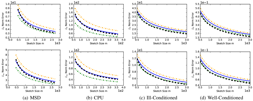
Figure 1: Numerical results for CS with extrapolation. The black dashed curve represents the ideal benchmark $\varepsilon_{\text{CS},m}(.05)$ described in the text. The average extrapolated estimate is shown in blue, with the yellow and green curves being one standard deviation away. Note: The upper row shows results for $\ell_{2}$ error ($\|\cdot\|_{\circ}=\|\cdot\|_{2}$), and the lower row shows results for $\ell_{\infty}$ error ($\|\cdot\|_{\circ}=\|\cdot\|_{\infty}$).

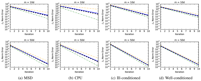
Figure 2: Numerical results for IHS with extrapolation. The black dashed curve represents the ideal benchmark $\varepsilon_{\text{IHS},i}(.05)$ described in the text. The average extrapolated estimate is shown in blue, with the yellow and green curves being one standard deviation away. The upper row shows results for $m=10d$, and the lower row shows results for $m=50d$.

Experiments for IHS.  The experiments for IHS were organized similarly to the case of CS, except that the sketch size $m$ was fixed (at either $m=10d$, or $m=50d$), and results were considered as a function of the iteration number. To be specific, the IHS algorithm was run 1,000 times, with $t=10$ total iterations on each run, and with SRHT sketching matrices being used at each iteration. For a given run, the successive error values $\|\hat{x}_{i}-x_{\textup{opt}}\|_{2}$ at $i=1,\dots,10$, were recorded. At each $i$, we computed the .95 sample quantile among the 1,000 error values, which is denoted as $\varepsilon_{\text{IHS},i}(.05)$, and is viewed as an ideal benchmark that satisfies ${\mathbb{P}}\big{(}\|\hat{x}_{i}-x_{\textup{opt}}\|_{2}\leq\varepsilon_{\text{IHS},i}(.05)\big{)}\approx.95$. In the plots, the value $\varepsilon_{\text{IHS},i}(.05)$ is plotted with the dashed black curve as a function of $i=1,\dots,10$. In addition, for each of the 1,000 runs, we applied Algorithm 2 at $i=1$ and $i=2$, producing 1,000 extrapolated values $\hat{\varepsilon}_{\text{extrap},i}(.05)$ at each $i\geq 3$. The averages of the extrapolated values are plotted in blue, and again, the yellow and green curves are obtained by adding or subtracting one standard deviation.

Comments on results for IHS. At a glance, Figure 2 shows that the extrapolated estimate stays on track with the ideal benchmark, and is a nearly unbiased estimate of $\varepsilon_{\text{IHS},i}(.05)$, for $i=3,\dots,10$. An interesting feature of the plots is how much the convergence rate of IHS depends on $m$. Specifically, we see that after 10 iterations, the choice of $m=10d$ versus $m=50d$ can lead to a difference in accuracy that is 4 or 5 orders of magnitude. This sensitivity to $m$ illustrates why selecting $t$ is a non-trivial issue in practice, and why the extrapolated estimate can provide a valuable source of extra information.

5 Conclusion

We have proposed a systematic approach to answer a very practical question that arises for randomized LS algorithms: “How accurate is a given solution?” A distinctive aspect of the method is that it leverages the bootstrap — a tool ordinarily used for statistical inference — in order to serve a computational purpose. To our knowledge, it is also the first error estimation method for randomized LS that is supported theoretical guarantees. Furthermore, the method does not add much cost to an underlying sketching algorithm, and it has been shown to perform well on several examples.

Acknowledgments

Lopes is partially supported by NSF grant DMS-1613218.

Outline of Appendices

The proof of Theorem 1 is decomposed into two parts, with the bounds for IHS and CS being handled in Appendices A and B respectively.

A Proof of Theorem 1 for Iterative Hessian Sketch

To make the structure of the proof clearer, the main ingredients are combined in Appendix A.1. The lower-level arguments are given in Appendix A.2.

Remark on notation.

Since we will often need to condition on the sketching matrices $S_{1},\dots,S_{t}$ in the IHS algorithm, we define $\mathcal{S}_{k}:=\{S_{1},\dots,S_{k}\}$ for any $1\leq k\leq t$, and put $\mathcal{S}_{0}:=\emptyset$.

A.1 High-level proof of the bound (23)

For any $\tau\in{\mathbb{R}}$, define the conditional distribution function

$$F_{n}(\tau):=\mathbb{P}\Big{(}\|\hat{x}_{t}-x_{\textup{opt}})\|_{\circ}\leq\tau\Big{\bracevert}\mathcal{S}_{t-1}\Big{)}.$$

Next, let $\varepsilon_{1}^{*},\dots,\varepsilon_{B}^{*}$ be the samples generated by Algorithm 2, and define the empirical distribution function

$$\hat{F}_{n,B}(\tau):=\textstyle\frac{1}{B}\textstyle\sum_{l=1}^{B}1\{\varepsilon_{l}^{*}\leq\tau\}.$$

In Proposition 2 below, we show that as $n\to\infty$,

$$\sup_{\tau\in{\mathbb{R}}}\Big{|}\hat{F}_{n,B}(\tau)-F_{n}(\tau)\Big{|}\to 0\text{ \ \ \ in \ $\mathbb{P}(\cdot\,|\mathcal{S}_{t-1})$-probability}.$$ (24)

Establishing this limit is the most difficult part of the proof. Next, for any number $p\in(0,1)$, and any distribution function $G$, define the quantile function $G^{-1}(p)=\inf\{\tau:G(\tau)\geq p\}$. Using this definition, as well as the limit (24), it follows that for any fixed $\delta\in(0,1-\alpha)$, the event

$$\mathcal{E}_{n}(\delta):=\Big{\{}\hat{\varepsilon}_{t}(\alpha)\geq F_{n}^{-1}(1-\alpha-\delta)\Big{\}}$$ (25)

satisfies

$$\mathbb{P}(\mathcal{E}_{n}(\delta)|\mathcal{S}_{t-1})\to 1,$$ (26)

and handful of details for checking this are given immediately after the end of this proof. We now use the event $\mathcal{E}_{n}(\delta)$ to derive an upper bound on the probability $\mathbb{P}\big{(}\|\hat{x}_{t}-x_{\textup{opt}}\|_{\circ}>\hat{\varepsilon}_{t}(\alpha)\big{|}\mathcal{S}_{t-1}\big{)}$. From the definition of $\mathcal{E}_{n}(\delta)$, it follows that

$$\mathbb{P}\Big{(}\|\hat{x}_{t}-x_{\textup{opt}}\|_{\circ}>\hat{\varepsilon}_{t}(\alpha)\Big{|}\mathcal{S}_{t-1}\Big{)}$$

$$=\;\mathbb{P}\Big{(}\Big{\{}\|\hat{x}_{t}-x_{\textup{opt}}\|_{\circ}>\hat{\varepsilon}_{t}(\alpha)\Big{\}}\cap\mathcal{E}_{n}(\delta)\Big{|}\mathcal{S}_{t-1}\Big{)}\,+\,\mathbb{P}\Big{(}\Big{\{}\|\hat{x}_{t}-x_{\textup{opt}}\|_{\circ}>\hat{\varepsilon}_{t}(\alpha)\Big{\}}\cap\mathcal{E}_{n}^{c}(\delta)\Big{|}\mathcal{S}_{t-1}\Big{)}$$

$$\leq\;\mathbb{P}\Big{(}\|\hat{x}_{t}-x_{\textup{opt}}\|_{\circ}>F_{n}^{-1}(1-\alpha-\delta)\Big{|}\mathcal{S}_{t-1}\Big{)}\,+\,\mathbb{P}(\mathcal{E}_{n}^{c}(\delta)|\mathcal{S}_{t-1})$$

$$=\;1-F_{n}\Big{(}F_{n}^{-1}(1-\alpha-\delta)\Big{)}\,+\,\mathbb{P}(\mathcal{E}_{n}^{c}(\delta)|\mathcal{S}_{t-1})$$

$$\leq\;\alpha+\delta+\mathbb{P}(\mathcal{E}_{n}^{c}(\delta)|\mathcal{S}_{t-1}),$$

and in the last step we have used the basic fact $F_{n}(F_{n}^{-1}(p))\geq p$ for any $p\in(0,1)$. So, by taking the complement of the event $\{\|\hat{x}_{t}-x_{\textup{opt}}\|_{\circ}>\hat{\varepsilon}_{t}(\alpha)\}$, the previous bounds give

$$\mathbb{P}\Big{(}\|\hat{x}_{t}-x_{\textup{opt}}\|_{\circ}\ \leq\ \hat{\varepsilon}_{t}(\alpha)\Big{|}\mathcal{S}_{t-1}\Big{)}\geq 1-\alpha-\delta-\mathbb{P}(\mathcal{E}_{n}^{c}(\delta)|\mathcal{S}_{t-1}).$$ (27)

Taking the expectation of both sides with respect to $\mathcal{S}_{t-1}$ leads to

$$\mathbb{P}\Big{(}\|\hat{x}_{t}-x_{\textup{opt}}\|_{\circ}\ \leq\ \hat{\varepsilon}_{t}(\alpha)\Big{)}\geq 1-\alpha-\delta-\mathbb{P}(\mathcal{E}_{n}^{c}(\delta)).$$ (28)

Then, taking $\liminf_{n\to\infty}$ on both sides with $\delta$ held fixed, and noting that that $\mathbb{P}(\mathcal{E}_{n}^{c}(\delta))\to 0$ (by the dominated convergence theorem and the limit (26)), we obtain

$$\liminf_{n\to\infty}\mathbb{P}\Big{(}\|\hat{x}_{t}-x_{\textup{opt}}\|_{\circ}\ \leq\ \hat{\varepsilon}_{t}(\alpha)\Big{)}\geq 1-\alpha-\delta.$$ (29)

Since the left side above does not depend on the arbitrarily small number $\delta$, it follows that

$$\liminf_{n\to\infty}\mathbb{P}\Big{(}\|\hat{x}_{t}-x_{\textup{opt}}\|_{\circ}\ \leq\ \hat{\varepsilon}_{t}(\alpha)\Big{)}\geq 1-\alpha,$$ (30)

and this implies the inequality (23). $\square$

Details for showing (26).

Due to the fact that $\hat{\varepsilon}_{t}(\alpha)$ can be expressed as $\hat{F}_{n,B}^{-1}(1-\alpha)$, we have the basic inequality $\hat{F}_{n,B}(\hat{\varepsilon}_{t}(\alpha))\geq 1-\alpha$. Also, if we define $\hat{\delta}_{n}:=|\hat{F}_{n,B}(\hat{\varepsilon}_{t}(\alpha))-F_{n}(\hat{\varepsilon}_{t}(\alpha))|$, then

$$\begin{split}F_{n}(\hat{\varepsilon}_{t}(\alpha))&\geq\hat{F}_{n,B}(\hat{\varepsilon}_{t}(\alpha))-\hat{\delta}_{n}\\[5.69046pt] &\geq 1-\alpha-\hat{\delta}_{n}.\end{split}$$ (31)

Next, the limit (24) ensures that for any fixed $\delta\in(0,1-\alpha)$, the event $\mathcal{E}_{n}^{\prime}(\delta):=\{\hat{\delta}_{n}\leq\delta\}$ satisfies $\mathbb{P}(\mathcal{E}_{n}^{\prime}|\mathcal{S}_{t-1})\to 1$. Furthermore, in light of the inquality (31) it is simple to check that $\mathcal{E}_{n}^{\prime}(\delta)\subset\mathcal{E}_{n}(\delta)$, which implies (26).

Proposition 2

If the conditions of Theorem 1 hold, then the limit (24) holds.

Proof Let $\|\hat{x}_{t}^{*}-\hat{x}_{t}\|_{\circ}$ be a bootstrap sample generated by Algorithm 2, and for any $\tau\in{\mathbb{R}}$, define the conditional distribution function

$$\hat{F}_{n}(\tau):=\mathbb{P}\Big{(}\|\hat{x}_{t}^{*}-\hat{x}_{t}\|_{\circ}\leq\tau\Big{|}\mathcal{S}_{t}\Big{)}.$$ (32)

(Note that the set $\mathcal{S}_{t}$ has been conditioned on here, which means that $\hat{F}_{n}$ is a random function with respect to $\mathbb{P}(\cdot\,|\mathcal{S}_{t-1})$.) Another important observation is that the bootstrap samples $\varepsilon_{1}^{*},\dots,\varepsilon_{B}^{*}$ may be regarded as i.i.d. draws from $\hat{F}_{n}$. Due to the Dvoretzky-Kiefer-Wolfowitz inquality (Dvoretzky et al., 1956, Massart, 1990), if $B\to\infty$ with $n\to\infty$, then

$$\sup_{\tau\in{\mathbb{R}}}\Big{|}\hat{F}_{n,B}(\tau)-\hat{F}_{n}(\tau)\Big{|}\to 0\text{ \ \ \ in \ \ $\mathbb{P}(\cdot\,|\mathcal{S}_{t-1})$-probability.}$$ (33)

(Note that this holds regardless of the rate at which $B$ diverges, and so no conditions on the relative sizes of $B$ and $n$ are needed.) So, due to the simple inequality

$$\sup_{\tau\in{\mathbb{R}}}\Big{|}\hat{F}_{n,B}(\tau)-F_{n}(\tau)\Big{|}\ \leq\ \sup_{\tau\in{\mathbb{R}}}\Big{|}\hat{F}_{n,B}(\tau)-\hat{F}_{n}(\tau)\Big{|}\ +\ \sup_{\tau\in{\mathbb{R}}}\Big{|}\hat{F}_{n}(\tau)-F_{n}(\tau)\Big{|},$$

the proof reduces to showing that

$$\sup_{\tau\in{\mathbb{R}}}\Big{|}\hat{F}_{n}(\tau)-F_{n}(\tau)\Big{|}\to 0\text{ \ \ \ in \ \ $\mathbb{P}(\,\cdot\,|\mathcal{S}_{t-1})$-probability,}$$ (34)

and this is the core aspect of the proof. This limit follows directly from Lemma 6, which can be found at the end of the next subsection. (Prior to Lemma 6, there are three other lemmas that assemble the main arguments.) $\square$

A.2 Lemmas supporting the proof of Proposition 2

In this section we will use some specialized notation. In addition, our proofs will rely on the convergence of conditional distributions, as reviewed below.

Notation for vectors and matrices.

We use $e_{1},\dots,e_{d}$ to refer to the standard basis vectors in ${\mathbb{R}}^{d}$. Next, we define two basic operations $\textup{uvec}(\cdot)$ and $\textup{sym}(\cdot)$ on matrices and vectors. For a symmetric matrix $M\in{\mathbb{R}}^{d\times d}$, let $\textup{uvec}(M)\in{\mathbb{R}}^{d(d+1)/2}$ be the vector obtained by extracting the upper triangular portion of $M$, where the entries of $\textup{uvec}(M)$ are ordered row-wise (starting from the first row). For example,

$$M=\begin{pmatrix}m_{11}&m_{12}\\ m_{21}&m_{22}\end{pmatrix}\ \ \ \Longrightarrow\ \ \ \textup{uvec}(M)=(m_{11},m_{12},m_{22}).$$

Next, for any vector $u\in{\mathbb{R}}^{d(d+1)/2}$, let $\textup{sym}(u)$ be the unique symmetric matrix in ${\mathbb{R}}^{d\times d}$ that satisfies $\textup{uvec}(\textup{sym}(u))=u$. For example,

$$u=(u_{1},u_{2},u_{3})\ \ \ \Longrightarrow\ \ \ \text{sym}(u)=\begin{pmatrix}u_{1}&u_{2}\\ u_{2}&u_{3}\end{pmatrix}.$$

Define the normalized matrix $\bar{A}_{n}:=\frac{1}{\sqrt{n}}A$, as well as the following analogues of $H_{n}=\frac{1}{n}A^{\top}A$,

$$\tilde{H}_{n}:=\textstyle\frac{1}{n}A^{\top}S_{t}^{\top}S_{t}A\ \ \ \ \text{ and }\ \ \ \tilde{H}_{n}^{*}:=\textstyle\frac{1}{n}A^{\top}S_{t}^{*\top}S_{t}^{*}A.$$ (35)

Lastly, when referring to the rows of $\sqrt{m}S_{t}$, we will omit the dependence on $t$ and write simply $s_{1},\dots,s_{m}$ for ease of notation.

Convergence of conditional distributions.

If a sequence of random vectors $V_{n}$ converges in distribution to a random vector $V$, we write $\mathcal{L}(V_{n})\xrightarrow{\ d\ }\mathcal{L}(V)$. In some situations, we will also need to discuss convergence of conditional distributions. To review the meaning of this notion, let $d_{\text{LP}}(\mathcal{L}(V_{n}),\mathcal{L}(V))$ denote the Lévy-Prohorov distance (Dudley, 2002, p. 394) between the distributions $\mathcal{L}(V_{n})$ and $\mathcal{L}(V)$, and note the basic fact that $d_{\text{LP}}(\mathcal{L}(V_{n}),\mathcal{L}(V))\to 0$ if and only if $\mathcal{L}(V_{n})\xrightarrow{\ d\ }\mathcal{L}(V)$. Now, suppose $U_{n}$ is another sequence of random vectors, and let $d_{\text{LP}}(\mathcal{L}(V_{n}|U_{n}),\mathcal{L}(V|U_{n}))$ denote the $d_{\text{LP}}$ distance between $\mathcal{L}(V_{n}|U_{n})$ and $\mathcal{L}(V|U_{n})$, which are random probability distributions. Likewise, the sequence $\{d_{\text{LP}}(\mathcal{L}(V_{n}|U_{n}),\mathcal{L}(V|U_{n}))\}_{n=1}^{\infty}$ may be regarded as a sequence of scalar random variables, and if it happens that this sequence converges to 0 in probability, then we say ‘$\mathcal{L}(V_{n}|U_{n})\xrightarrow{\ d\ }\mathcal{L}(V|U_{n})\text{ in probability}$’.

The rest of this subsection consists of the four lemmas needed to prove Proposition 2.

Lemma 3

Suppose the conditions of Theorem 1 hold. Then, there is a mean-zero random vector $V\in{\mathbb{R}}^{d(d+1)/2}$ with a multivariate normal distribution and a positive definite covariance matrix, such that as $n\to\infty$,

$$\mathcal{L}\big{\{}\sqrt{m}(\textup{uvec}(\tilde{H}_{n})-\textup{uvec}(H_{n}))\big{\}}\xrightarrow{\ d\ }\mathcal{L}(V).$$ (36)

Proof. Due to the Cramér-Wold theorem (van der Vaart, 1998), it sufficient to show that for any fixed non-zero vector $c\in{\mathbb{R}}^{d(d+1)/2}$, the scalar random variable $\langle\sqrt{m}(\textup{uvec}(\tilde{H}_{n})-\textup{uvec}(H_{n})),c\rangle$ converges in distribution to a zero-mean Gaussian random variable with positive variance. It is clear that for any such vector $c$, there is a corresponding upper triangular matrix $C\in{\mathbb{R}}^{d\times d}$ such that

$$\small\begin{split}\langle\sqrt{m}(\textup{uvec}(\tilde{H}_{n})-\textup{uvec}(H_{n})),c\rangle\ &=\ \sqrt{m}\big{(}\mathrm{tr}(\tilde{H}_{n}C)-\mathrm{tr}(H_{n}C)\big{)}\\[5.69046pt] &=\frac{1}{\sqrt{m}}\sum_{i=1}^{m}\Big{(}s_{i}^{\top}\bar{A}_{n}C\bar{A}_{n}^{\top}s_{i}-\mathrm{tr}(\bar{A}_{n}C\bar{A}_{n}^{\top})\Big{)},\\[5.69046pt] &=\frac{1}{\sqrt{m}}\sum_{i=1}^{m}\xi_{i,n}\end{split}$$ (37)

where we define the random variable $\xi_{i,n}:=s_{i}^{\top}\bar{A}_{n}C\bar{A}_{n}^{\top}s_{i}-\mathrm{tr}(\bar{A}_{n}C\bar{A}_{n}^{\top})$. It is also clear that $\xi_{1,n},\dots,\xi_{m,n}$ are i.i.d. with mean zero.

As a preparatory step towards applying the central limit theorem, we now show that $\mathsf{var}(\xi_{1,n})$ converges to a positive limit. Because each vector $s_{i}$ is composed of i.i.d. random variables, we may use an exact formula for the variance of quadratic forms (Bai and Silverstein, 2004, eqn. 1.15), which leads to

$$\mathsf{var}(\xi_{1,n}) =\mathsf{var}\Big{(}s_{1}^{\top}\bar{A}_{n}C\bar{A}_{n}^{\top}s_{1}\Big{)}$$ (38)

$$=2\big{\|}\bar{A}_{n}C\bar{A}_{n}^{\top}\big{\|}_{F}^{2}+(\kappa-3)\sum_{j=1}^{n}(e_{j}^{\top}\bar{A}_{n}C\bar{A}_{n}^{\top}e_{j})^{2},$$ (39)

where we recall that $\kappa:=\mathbb{E}[s_{i,j}^{4}]$ does not depend on $n$. Next, observe that the relation $\|\bar{A}_{n}C\bar{A}_{n}^{\top}\|_{F}^{2}=\mathrm{tr}(CH_{n}CH_{n})$ implies that $\|\bar{A}_{n}C\bar{A}_{n}^{\top}\|_{F}^{2}\to\|H_{\infty}^{1/2}CH_{\infty}^{1/2}\|_{F}^{2}$, and also, the second term in line (39) converges to a limit, say $(\kappa-3)\ell(C)$, due to Assumption 1. Hence,

$$\mathsf{var}(\xi_{1,n})\to 2\|H_{\infty}^{1/2}CH_{\infty}^{1/2}\|_{F}^{2}+(\kappa-3)\ell(C).$$ (40)

Now that we have shown $\mathsf{var}(\xi_{1,n})$ converges to a limit, we verify that this limit is positive. Since we assume $\kappa>1$, it is clear that $\kappa-3>{\epsilon}_{0}-2$ for some fixed ${\epsilon}_{0}\in(0,1)$. Also, since the second term in line (39) represents the sum of the squares of the diagonal entries of $\bar{A}_{n}C\bar{A}_{n}^{\top}$, the sum of the two terms must be at least ${\epsilon}_{0}\|\bar{A}_{n}C\bar{A}_{n}^{\top}\|_{F}^{2}$. Therefore, the limit of $\mathsf{var}(\xi_{1,n})$ is lower-bounded by ${\epsilon}_{0}\|H_{\infty}^{1/2}CH_{\infty}^{1/2}\|_{F}^{2}$, and because $H_{\infty}$ is positive definite, this lower bound is positive when $C\neq 0.$

Given that $\mathsf{var}(\xi_{1,n})$ converges to a positive limit, we now apply the central limit theorem. More specifically, since the common distribution of the variables $\{\xi_{1,n},\dots,\xi_{m,n}\}$ changes with $n$, we use the Lindeberg central limit theorem for triangular arrays (van der Vaart, 1998, Prop. 2.27). In addition to the existence of a limit for $\mathsf{var}(\xi_{1,n})$, this theorem requires that the limit $\mathbb{E}\big{[}\xi_{1,n}^{2}1\{|\xi_{1,n}|>{\epsilon}\sqrt{m}\}\big{]}\to 0$ holds for any fixed ${\epsilon}>0$ as $n\to\infty$. To verify this condition, the Cauchy-Schwarz inequality gives

$$\mathbb{E}\big{[}\xi_{1,n}^{2}1\{|\xi_{1,n}|>{\epsilon}\sqrt{m}\}\big{]}\ \leq\sqrt{\mathbb{E}[\xi_{1,n}^{4}]}\cdot\sqrt{\mathbb{P}(\xi_{1,n}>{\epsilon}\sqrt{m})}.$$ (41)

In turn, using a classical bound for moments of random quadratic forms  (Bai and Silverstein, 2010, Lemma B.26), and the assumption that $\mathbb{E}[s_{i,j}^{8}]<\infty$, it is straightforward to check that $\mathbb{E}[\xi_{1,n}^{4}]=\mathcal{O}(1)$. Also, the condition $\mathbb{P}(\xi_{1,n}>{\epsilon}\sqrt{m})\to 0$ follows from Chebychev’s inequality and the limit (40). Therefore, the Lindeberg central limit theorem implies

$$\mathcal{L}(\langle\sqrt{m}(\textup{uvec}(\tilde{H}_{n})-\textup{uvec}(H_{n})),c\rangle)\xrightarrow{\ d\ }N(0,\sigma^{2}(C)),$$ (42)

where we put $\sigma^{2}(C):=2\|H_{\infty}^{1/2}CH_{\infty}^{1/2}\|_{F}^{2}+(\kappa-3)\ell(C)$. This proves the limit (36). $\square$

Lemma 4

Suppose the conditions of Theorem 1 hold, and let $V$ be the random vector in statement of Lemma 3. Then, as $n\to\infty$,

$$\mathcal{L}\big{\{}\sqrt{m}(\textup{uvec}(\tilde{H}_{n}^{*})-\textup{uvec}(\tilde{H}_{n}))\big{\bracevert}S_{t}\big{\}}\xrightarrow{\ d\ }\mathcal{L}(V),\ \text{ in probability}.$$ (43)

Remark.

Note that the second limit holds in probability because $\mathcal{L}\big{\{}\sqrt{m}(\textup{uvec}(\tilde{H}_{n}^{*})-\textup{uvec}(\tilde{H}_{n}))\big{\bracevert}S_{t}\big{\}}$ is a random probability distribution that depends on $S_{t}$.

Proof The overall approach is similar to the proof of Lemma 3. If we let $s_{1}^{*},\dots,s_{m}^{*}$ be drawn with replacement from $\{s_{1},\dots,s_{m}\}$, then it is simple to check that $\tilde{H}_{n}$ can be represented as

$$\tilde{H}_{n}^{*}=\frac{1}{m}\sum_{i=1}^{m}\bar{A}_{n}^{\top}s_{i}^{*}s_{i}^{*\top}\bar{A}_{n}.$$

Accordingly, for any $c\in{\mathbb{R}}^{d(d+1)/2}$ we have

$$\begin{split}\Big{\langle}\sqrt{m}(\textup{uvec}(\tilde{H}_{n}^{*})-\textup{uvec}(\tilde{H}_{n})),c\Big{\rangle}\ &=\ \frac{1}{\sqrt{m}}\sum_{i=1}^{m}\xi_{i,n}^{*},\end{split}$$ (44)

where $\xi_{i,n}^{*}:=s_{i}^{*\top}\bar{A}_{n}C\bar{A}_{n}^{\top}s_{i}^{*}-\mathrm{tr}(C\tilde{H}_{n})$, and $C$ is the upper-triangular matrix associated with $c$. Our goal is now to show that conditionally on the matrix $S_{t}$, the sum $\frac{1}{\sqrt{m}}\sum_{i=1}^{m}\xi_{i,n}^{*}$ satisfies the conditions of the Lindeberg central limit theorem (in probability), which will lead to the desired limit (43). To do this, first observe that conditionally on $S_{t}$, the random variables $\xi_{1}^{*},\dots,\xi_{m}^{*}$ are i.i.d., and satisfy $\mathbb{E}[\xi_{i,n}^{*}|S_{t}]=0$. It remains to verify the following two conditions,

$$\mathsf{var}(\xi_{1,n}^{*}|S_{t})\to\sigma^{2}(C)\ \text{ in probability},$$ (45)

where $\sigma^{2}(C)$ is as defined beneath line (42), and also

$$\mathbb{E}[(\xi_{1,n}^{*})^{2}1\{|\xi_{1,n}^{*}>{\epsilon}\sqrt{m}\}\,|S_{t}]\to 0\text{ \ \ \ in probability},$$ (46)

for any fixed ${\epsilon}>0$.

To verify the limit (45), note that because $\xi_{1,n}^{*},\dots,\xi_{m,n}^{*}$ can be viewed as samples with replacement from the set $\{\xi_{1,n},\dots,\xi_{m,n}\}$, it follows that

$$\mathsf{var}(\xi_{1,n}^{*}|S_{t})=\hat{\varsigma}_{n}^{\,2},$$ (47)

where $\hat{\varsigma}_{n}^{2}$ denotes the sample variance $\hat{\varsigma}_{n}^{\,2}:=\frac{1}{m}\sum_{i=1}^{m}(\xi_{i,n}-\bar{\xi})^{2},$ and $\bar{\xi}:=\frac{1}{m}\sum_{i=1}^{m}\xi_{i,n}$. It is clear that $\hat{\varsigma}^{\,2}_{n}$ is asymptotically unbiased for $\sigma^{2}(C)$, since $\mathbb{E}[\hat{\varsigma}^{\,2}_{n}]=\textstyle\frac{m-1}{m}\mathsf{var}(\xi_{1,n})$. So, to show that $\hat{\varsigma}^{\,2}_{n}$ converges to $\sigma^{2}(C)$ in probability, it is enough to show that $\mathsf{var}(\hat{\varsigma}^{\,2}_{n})$ converges to 0. Using a classical formula for the variance of $\hat{\varsigma}_{n}$ (Kenney and Keeping, 1951, p.164), it is simple to obtain the bound

$$\mathsf{var}(\hat{\varsigma}^{\,2}_{n})\ =\mathcal{O}\Big{(}\frac{1}{n}\frac{\mu_{4,n}}{\mathsf{var}(\xi_{1,n})^{2}}\Big{)},$$ (48)

where $\mu_{4,n}$ is the fourth central moment of $\xi_{1,n}$, i.e.

$$\mu_{4,n}=\mathbb{E}\Big{[}\big{(}\xi_{1,n}-\mathbb{E}[\xi_{1,n}]\big{)}^{4}\Big{]}.$$

Using a general bound for the moments of quadratic forms (Bai and Silverstein, 2010, Lemma B.26), this quantity can be bounded as

$$\mu_{4,n}=\mathcal{O}\Big{(}\mathrm{tr}(M_{n})^{2}+\mathrm{tr}(M_{n}^{2})\Big{)}$$ (49)

where $M_{n}:=(\bar{A}_{n}C\bar{A}_{n}^{\top})^{2}$. Since both of the traces above can be expressed in terms of the matrix $C\bar{A}_{n}^{\top}\bar{A}_{n}$, which converges to $CH_{\infty}$, it follows that $\mu_{4,n}=\mathcal{O}(1)$. Also, it was shown in the proof of Lemma 3 that $\mathsf{var}(\xi_{1,n})$ has a positive limit. Altogether, this completes the work needed to prove the limit (45).

Finally, to verify limit (46), observe that since $\mathbb{E}\big{[}(\xi_{1,n}^{*})^{2}1\{|\xi_{1,n}^{*}>{\epsilon}\sqrt{m}\}\,\big{|}S_{t}\big{]}$ is a non-negative random variable, Markov’s inequality ensures that convergence to 0 in expectation implies convergence to 0 in probability. Using the fact that $\xi_{1,n}^{*}$ is sampled with replacement from the set $\{\xi_{1,n},\dots,{\bf x}_{m,n}\}$, we have

$$\mathbb{E}\big{[}(\xi_{1,n}^{*})^{2}1\{|\xi_{1,n}^{*}>{\epsilon}\sqrt{m}\}\,\big{|}S_{t}\big{]}=\frac{1}{m}\sum_{i=1}^{m}\xi_{i,n}^{2}1\{\xi_{i,n}>{\epsilon}\sqrt{m}\},$$ (50)

and so

$$\mathbb{E}\Big{[}\mathbb{E}\big{[}(\xi_{1,n}^{*})^{2}1\{|\xi_{1,n}^{*}>{\epsilon}\sqrt{m}\}\,\big{|}S_{t}\big{]}\Big{]}=\mathbb{E}\big{[}\xi_{1,n}^{2}1\{\xi_{1,n}>{\epsilon}\sqrt{m}\}\big{]}.$$

Consequently, the argument based on the bound (41) in the proof of Lemma 3 may be re-used to show that the right hand side above tends to 0. $\square$

Remarks on notation.

For the following lemma, let $\mathcal{U}\subset{\mathbb{R}}^{d(d+1)/2}$ denote the set of all vectors $u$ that can be represented as $u=\textup{uvec}(M)$ for some symmetric invertible matrix $M\in{\mathbb{R}}^{d\times d}$. In this notation, we define the map $\phi:\mathcal{U}\to\mathcal{U}$ by

$$\phi(u)=\textup{uvec}(\textup{sym}(u)^{-1}).$$

Lemma 5

Suppose the conditions of Theorem 1 hold. Then there is a mean-zero multivariate normal random vector $W\in{\mathbb{R}}^{d(d+1)/2}$ with a positive definite covariance matrix such that as $n\to\infty$,

$$\mathcal{L}\Big{\{}\sqrt{m}\Big{(}\phi(\textup{uvec}(\tilde{H}_{n}))-\phi(\textup{uvec}(H_{n}))\Big{)}\Big{\}}\xrightarrow{\ d\ }\mathcal{L}(W),$$ (51)

and

$$\mathcal{L}\Big{\{}\sqrt{m}\Big{(}\phi(\textup{uvec}(\tilde{H}_{n}^{*}))-\phi(\textup{uvec}(\tilde{H}_{n}))\Big{)}\Big{\bracevert}S_{t}\Big{\}}\xrightarrow{\ d\ }\mathcal{L}(W)\ \text{ in probability}.$$ (52)

Proof Recall that we assume $\sqrt{m}(H_{n}-H_{\infty})\to 0$, where $H_{\infty}$ is positive definite. Since the map $\phi$ is differentiable, it follows from the delta method (van der Vaart, 1998, Theorem 3.1) and Lemma 3 that

$$\mathcal{L}\big{(}\sqrt{m}(\phi(\textup{uvec}(\tilde{H}_{n}))-\phi(\textup{uvec}(H_{n})))|S_{t})\xrightarrow{\ d\ }\mathcal{L}(W),\text{ \ \ in probability}$$

where we define $W:=\phi^{\prime}_{0}(V),$ with $V$ being the random vector in Lemma 3, and $\phi^{\prime}_{0}$ denoting the differential of $\phi$ at the point $\textup{uvec}(H_{\infty})$.

Due to Lemma 3, we know that $V$ has a multivariate normal distribution with mean zero and a positive-definite covariance matrix. Also, because the map $\phi$ and its inverse $\phi^{-1}$ are differentiable on $\mathcal{U}$, it follows that the differential $\phi^{\prime}_{0}$ must be an invertible linear map on ${\mathbb{R}}^{d(d+1)/2}$. Consequently, the random vector $W=\phi_{0}^{\prime}(V)$ has a positive definite covariance matrix. Finally, the same reasoning can be used to obtain the limit (52), since the limit (43) holds almost surely along subsequences, and the delta method may be applied again with the map $\phi$ (cf. van der Vaart (1998, Theorem 23.5)) . $\square$

Lemma 6

Suppose the conditions of Theorem 1 hold, and let $Z=\textup{sym}(W)$, with $W$ being random vector in the statement of Lemma 5. Then, for almost every sequence of sets $\mathcal{S}_{t-1}$, the following limit holds as $n\to\infty$,

$$\sup_{\tau\in{\mathbb{R}}}\bigg{|}\mathbb{P}\Big{(}\sqrt{m}\|\hat{x}_{t}-x_{\textup{opt}}\|_{\circ}\leq\tau\big{\bracevert}\mathcal{S}_{t-1}\Big{)}-\mathbb{P}\Big{(}\textstyle\frac{1}{n}\|Zg_{t-1}\|_{\circ}\leq\tau\big{\bracevert}\mathcal{S}_{t-1}\Big{)}\bigg{|}\to 0.$$ (53)

Furthermore,

$$\sup_{\tau\in{\mathbb{R}}}\bigg{|}\mathbb{P}\Big{(}\sqrt{m}\|\hat{x}_{t}^{*}-\hat{x}_{t}\|_{\circ}\leq\tau\big{\bracevert}\mathcal{S}_{t}\Big{)}-\mathbb{P}\Big{(}\textstyle\frac{1}{n}\|Zg_{t-1}\|_{\circ}\leq\tau\big{\bracevert}\mathcal{S}_{t-1}\Big{)}\bigg{|}\to 0,\ \text{ in \ $\mathbb{P}(\cdot\,|\mathcal{S}_{t-1})$-probability}.$$ (54)

Proof We first prove the limit (53). For any fixed vector $v\in{\mathbb{R}}^{d}$, and fixed scalar $\tau$, define the set $\mathcal{C}(v,\tau)\subset{\mathbb{R}}^{d(d+1)/2}$ to contain the vectors $u$ satisfying $\|\textup{sym}(u)v\|_{\circ}\leq\tau$. Based on this definition of $\mathcal{C}(v,\tau)$, the following events are equal

$$\big{\{}\textstyle\frac{1}{n}\|Zg_{t-1}\|_{\circ}\leq\tau\big{\}}=\big{\{}\textup{uvec}(Z)\in\mathcal{C}(g_{t-1},n\tau)\big{\}}.$$ (55)

Next, using the relation

$$\hat{x}_{t}-x_{\textup{opt}}=-\textstyle\frac{1}{n}\big{(}\tilde{H}_{n}^{-1}-H_{n}^{-1}\big{)}g_{t-1},$$

it straightforward to check that the following events are also equal

$$\Big{\{}\sqrt{m}\|\hat{x}_{t}-x_{\textup{opt}}\|_{\circ}\leq\tau\Big{\}}=\Big{\{}\sqrt{m}\Big{(}\phi(\textup{uvec}(\tilde{H}_{n}))-\phi(\textup{uvec}(H_{n}))\Big{)}\in\mathcal{C}(g_{t-1},n\tau)\Big{\}}.$$ (56)

To proceed, we make use of the observation that the set $\mathcal{C}(g_{t-1},n\tau)$ is always convex and (Borel) measurable. Likewise, if we let $\mathscr{C}_{\text{convex}}$ denote the collection of all measurable convex subsets of ${\mathbb{R}}^{d(d+1)/2}$, it follows that the following supremum over $\tau\in{\mathbb{R}}$

$$\sup_{\tau\in{\mathbb{R}}}\bigg{|}\mathbb{P}\Big{(}\sqrt{m}\|\hat{x}_{t}-x_{\textup{opt}}\|_{\circ}\leq\tau\Big{\bracevert}\mathcal{S}_{t-1}\Big{)}-\mathbb{P}\Big{(}\textstyle\frac{1}{n}\|Zg_{t-1}\|_{\circ}\leq\tau\Big{\bracevert}\mathcal{S}_{t-1}\Big{)}\bigg{|}$$ (57)

is upper bounded by the following supremum over $\mathcal{C}\in\mathscr{C}_{\text{convex}}$,

$$\ \sup_{\mathcal{C}\in\mathscr{C}_{\text{convex}}}\bigg{|}\mathbb{P}\Big{(}\sqrt{m}\Big{(}\phi(\textup{uvec}(\tilde{H}_{n}))-\phi(\textup{uvec}(H_{n}))\Big{)}\in\mathcal{C}\Big{\bracevert}\mathcal{S}_{t-1}\Big{)}-\mathbb{P}(\textup{uvec}(Z)\in\mathcal{C}\big{\bracevert}\mathcal{S}_{t-1})\bigg{|}.$$ (58)

To conclude the proof of (53), it suffices to show that the previous expression converges to 0 as $n\to\infty$. For this purpose, we apply the general fact that if a sequence of random vectors $\zeta_{n}$ converges in distribution to a random vector $\zeta$, and if $\zeta$ has a multivariate normal distribution with a positive definite covariance matrix, then

$$\ \sup_{\mathcal{C}\in\mathscr{C}_{\text{convex}}}\Big{|}\mathbb{P}(\zeta_{n}\in\mathcal{C})-\mathbb{P}(\zeta\in\mathcal{C})\Big{|}\to 0.$$ (59)

(We refer to the book Bhattacharya and Rao (1986, Theorem 1.11) for further details.) Now, observe that $\tilde{H}_{n}$ is independent of $\mathcal{S}_{t-1}$, and Lemma 5 ensures that $\sqrt{m}\big{(}\phi(\textup{uvec}(\tilde{H}_{n}))-\phi(\textup{uvec}(H_{n}))\big{)}$ converges in distribution to $W=\textup{uvec}(Z)$, which is multivariate normal with a positive definite covariance matrix. Consequently, the conditioning on $\mathcal{S}_{t-1}$ may be dropped, and the limit (59) implies that the supremum in line (58) must converge to 0 as $n\to\infty$. Finally, the bootstrap limit (54) may be proven by repeating the same argument in conjunction with (52). $\square$

B Proof of Theorem 1 for Classic Sketch

B.1 High-level proof of the bound (22)

In analogy with Appendix A.1, let $\tau\in{\mathbb{R}}$, and define the following conditional distribution function

$$G_{n}(\tau):=\mathbb{P}\Big{(}\|\tilde{x}_{t}-x_{\textup{opt}}\|_{\circ}\leq\tau\Big{)}.$$

Also, letting $\varepsilon_{1}^{*},\dots,\varepsilon_{B}^{*}$ denote the samples generated by Algorithm 1, define

$$\hat{G}_{n}(\tau) :=\mathbb{P}\Big{(}\|\tilde{x}^{*}-\tilde{x}\|_{\circ}\leq\tau\Big{\bracevert}S\Big{)},$$ (60)

$$\hat{G}_{n,B}(\tau) :=\textstyle\frac{1}{B}\textstyle\sum_{l=1}^{B}1\{\varepsilon_{l}^{*}\leq\tau\}.$$ (61)

By using these functions in place of their IHS counterparts $F_{n}(\tau)$, $\hat{F}_{n}(\tau)$, and $\hat{F}_{n,B}(\tau)$, the argument at the beginning of Appendix A.1 can be essentially repeated to reach the conclusion

$$\liminf_{n\to\infty}\mathbb{P}\Big{(}\|\tilde{x}_{t}-x_{\textup{opt}}\|_{\circ}\ \leq\ \tilde{\varepsilon}(\alpha)\Big{)}\geq 1-\alpha,$$ (62)

which implies the desired inequality (22). The only part of the argument that needs to be updated is to prove the analogue of Proposition 2 for the case of CS. In other words, it suffices to show that

$$\sup_{\tau\in{\mathbb{R}}}\Big{|}\hat{G}_{n}(\tau)-G_{n}(\tau)\Big{|}\to 0\text{ \ \ \ in probability.}$$ (63)

Proving this limit will be handled with Proposition 8 below. $\square$

Remarks on notation.

The proof of Proposition 8 relies on the following preliminary result. To introduce some notation, we will use the normalized gradient vector $\texttt{g}_{n}:=\textstyle\frac{1}{n}A^{\top}b$, and the analogues

$$\tilde{\texttt{g}}_{n}:=\textstyle\frac{1}{n}\tilde{A}^{\top}\tilde{b},\text{ \ \ \ and \ \ \ }\tilde{\texttt{g}}_{n}^{*}:=\textstyle\frac{1}{n}(\tilde{A}^{*})^{\top}(\tilde{b}^{*}).$$

Note that $\texttt{g}_{n}$ is not the same as the gradient $g_{t}$ used previously in the context of IHS. One additional detail to clarify is that in this section, we will overload the notation introduced in line (35). Specifically, we re-define $\tilde{H}_{n}$ and $\tilde{H}_{n}^{*}$ in terms of the single sketching matrix $S$ for CS and its resampled version $S^{*}$ CS (rather than the matrices $S_{t}$ and $S_{t}^{*}$ used in the context of IHS). That is,

$$\tilde{H}_{n}:=\textstyle\frac{1}{n}A^{\top}S^{\top}SA\ \ \ \ \text{ and }\ \ \ \tilde{H}_{n}^{*}:=\textstyle\frac{1}{n}A^{\top}S^{*\top}S^{*}A.$$ (64)

Furthermore, the matrix $S$ has the same distribution as $S_{t}$, and so the Lemmas 3, 4 and 5, involving $\tilde{H}_{n}$ and $\tilde{H}_{n}^{*}$, apply to the CS context with no changes.

Lemma 7

Suppose the conditions of Theorem 1 hold. Then, there is a mean-zero random vector $Y\in{\mathbb{R}}^{d}$ having a multivariate normal distribution and a non-zero covariance matrix, such that as $n\to\infty$,

$$\mathcal{L}(\sqrt{m}(\tilde{x}-x_{\textup{opt}}))\xrightarrow{\ d\ \ }\mathcal{L}(Y),$$ (65)

and

$$\mathcal{L}(\sqrt{m}(\tilde{x}^{*}-\tilde{x})|S)\xrightarrow{\ d\ }\mathcal{L}(Y),\ \text{ in probability}.$$ (66)

Proof The proof of Lemmas 3 and 4 can be adapted to show that the following joint limits hold

$$\mathcal{L}\Big{\{}\sqrt{m}\Big{(}\big{(}\textup{uvec}(\tilde{H}_{n}),\tilde{\texttt{g}}_{n}\big{)}-\big{(}\textup{uvec}(H_{n}),\texttt{g}_{n}\big{)}\Big{)}\Big{\}}\xrightarrow{\ d\ }\mathcal{L}(V,U),$$ (67)

and

$$\mathcal{L}\Big{\{}\sqrt{m}\Big{(}\big{(}\textup{uvec}(\tilde{H}_{n}^{*}),\tilde{\texttt{g}}_{n}^{*}\big{)}-\big{(}\textup{uvec}(\tilde{H}_{n}),\tilde{\texttt{g}}_{n}\big{)}\Big{)}\Big{\bracevert}S\Big{\}}\xrightarrow{\ d\ }\mathcal{L}(V,U),$$ (68)

where $U\in{\mathbb{R}}^{d}$ is a random vector such that the concatenated vector $(V,U)\in{\mathbb{R}}^{d(d+1)/2}\times{\mathbb{R}}^{d}$ has a mean-zero multivariate normal distribution with a non-zero covariance matrix. To proceed, recall that $\mathcal{U}\subset{\mathbb{R}}^{d(d+1)/2}$ denotes the set of vectors that can be written as $\textup{uvec}(M)$ for some symmetric invertible matrix $M$. Also, recall that for any $u\in\mathcal{U}$, the expression $\textup{sym}(u)$ refers to the unique symmetric matrix in ${\mathbb{R}}^{d\times d}$ that satisfies $\textup{uvec}(\textup{sym}(u))=u$. Next, consider the map $\Phi:\mathcal{U}\times{\mathbb{R}}^{d}\to{\mathbb{R}}^{d}$ defined by

$$\Phi(u,v)=(\textup{sym}(u))^{-1}v,$$

as well as the following relations, which are straightforward to verify

$$\tilde{x}-x_{\textup{opt}}=\tilde{H}_{n}^{-1}\tilde{\texttt{g}}_{n}-H_{n}^{-1}\texttt{g}_{n}$$ (69)

$$\ \ \ \ \ \ \ \ \ \tilde{x}^{*}-\tilde{x}=(\tilde{H}_{n}^{*})^{-1}\tilde{\texttt{g}}_{n}^{*}-\tilde{H}_{n}^{-1}\tilde{\texttt{g}}_{n}.$$ (70)

These relations can be written in terms of the map $\Phi$ as

$$\sqrt{m}(\tilde{x}-x_{\textup{opt}})=\sqrt{m}\Big{(}\Phi\big{(}\textup{uvec}(\tilde{H}_{n}),\tilde{\texttt{g}}_{n}\big{)}-\Phi\big{(}\textup{uvec}(H_{n}),\texttt{g}_{n}\big{)}\Big{)},$$

and

$$\sqrt{m}(\tilde{x}^{*}-\tilde{x})=\sqrt{m}\Big{(}\Phi\big{(}\textup{uvec}(\tilde{H}_{n}^{*}),\tilde{\texttt{g}}_{n}^{*}\big{)}-\Phi\big{(}\textup{uvec}(\tilde{H}_{n}),\tilde{\texttt{g}}_{n}\big{)}\Big{)}.$$

Next, recall the assumptions $\sqrt{m}(H_{n}-H_{\infty})\to 0$ and $\sqrt{m}(\texttt{g}_{n}-\texttt{g}_{\infty})\to 0$, and note that the map $\Phi$ is differentiable. Consequently, it follows from the delta method (van der Vaart, 1998, Theorem 3.1), as well as the limit (67) that

$$\mathcal{L}(\sqrt{m}(\tilde{x}-x_{\textup{opt}}))\xrightarrow{\ \ d\ \ }\mathcal{L}(\Phi_{0}^{\prime}(V,U)),$$

where $\Phi_{0}^{\prime}$ denotes the differential of $\Phi$ evaluated at the point $(\textup{uvec}(H_{\infty}),\texttt{g}_{\infty})$. Furthermore, since $\Phi$ and $\Phi^{-1}$ are differentiable, it follows that $\Phi_{0}^{\prime}$ is an invertible linear map, which implies that the random vector $\Phi_{0}^{\prime}(V,U)$ has a non-zero covariance matrix (since $(V,U)$ does). Similarly, the delta method can be applied to the limit (68) to obtain

$$\mathcal{L}(\sqrt{m}(\tilde{x}^{*}-\tilde{x})|S)\xrightarrow{\ \ d\ \ }\mathcal{L}(\Phi_{0}^{\prime}(V,U)),\text{ in probability}.$$

Finally, letting $Y=\Phi_{0}^{\prime}(V,U)$ completes the proof. $\square$

Proposition 8

If the conditions of Theorem 1 hold, then the limit (63) holds

Proof Let $Y$ be the random vector in the statement of Lemma 7. Combining that lemma with the continuous mapping theorem (van der Vaart, 1998, Theorem 2.3), and the fact that any norm $\|\cdot\|_{\circ}$ on ${\mathbb{R}}^{d}$ is continuous, we have

$$\mathcal{L}(\sqrt{m}\|\tilde{x}-x_{\textup{opt}}\|_{\circ})\xrightarrow{\ d\ \ }\mathcal{L}(\|Y\|_{\circ}),$$ (71)

and

$$\mathcal{L}\big{(}\sqrt{m}\|\tilde{x}^{*}-\tilde{x}\|_{\circ}\big{\bracevert}S\big{)}\xrightarrow{\ d\ }\mathcal{L}(\|Y\|_{\circ}),\ \text{ in probability}.$$ (72)

Since the random vector $Y$ has a multivariate normal distribution with a non-zero covariance matrix, it is straightforward to show that the random variable $\|Y\|_{\circ}$ has a continuous distribution function. So, it follows from Polya’s theorem (Bickel and Doksum, 2007, Theorem B.7.7) that

$$\sup_{\tau\in{\mathbb{R}}}\Big{|}\mathbb{P}\Big{(}\sqrt{m}\|\tilde{x}-x_{\textup{opt}}\|_{\circ}\leq\tau\Big{)}-\mathbb{P}\big{(}\|Y\|_{\circ}\leq\tau\big{)}\Big{|}\to 0,$$ (73)

and

$$\ \ \ \ \ \ \ \ \ \ \ \ \ \ \ \ \ \ \ \ \ \sup_{\tau\in{\mathbb{R}}}\Big{|}\mathbb{P}\Big{(}\sqrt{m}\|\tilde{x}^{*}-\tilde{x}\|_{\circ}\leq\tau\Big{\bracevert}S\Big{)}-\mathbb{P}\big{(}\|Y\|_{\circ}\leq\tau\big{)}\Big{|}\to 0\text{ \ \ in probability},$$ (74)

which implies the limit (63) by the triangle inequality. $\square$

References

• Ahfock et al. (2017) D. Ahfock, W. J. Astle, and S. Richardson. Statistical properties of sketching algorithms. arXiv:1706.03665, 2017.
• Ailon and Chazelle (2006) N. Ailon and B. Chazelle. Approximate nearest neighbors and the fast Johnson-Lindenstrauss transform. In Annual ACM Symposium on Theory of Computing (STOC), 2006.
• Ailon and Liberty (2009) N. Ailon and E. Liberty. Fast dimension reduction using Rademacher series on dual BCH codes. Discrete & Computational Geometry, 42(4):615–630, 2009.
• Ainsworth and Oden (2011) M. Ainsworth and J. T. Oden. A Posteriori Error Estimation in Finite Element Analysis, volume 37. John Wiley & Sons, 2011.
• Avron et al. (2010) H. Avron, P. Maymounkov, and S. Toledo. Blendenpik: Supercharging LAPACK’s least-squares solver. SIAM Journal on Scientific Computing, 32(3):1217–1236, 2010.
• Bai and Silverstein (2004) Z. D. Bai and J. W. Silverstein. CLT for linear spectral statistics of large-dimensional sample covariance matrices. The Annals of Probability, 32:553–605, 2004.
• Bai and Silverstein (2010) Z. D. Bai and J. W. Silverstein. Spectral Analysis of Large Dimensional Random Matrices. Springer, New York, 2010.
• Bartels and Hennig (2016) S. Bartels and P. Hennig. Probabilistic approximate least-squares. In Artificial Intelligence and Statistics (AISTATS), 2016.
• Becker et al. (2017) S. Becker, B. Kawas, and M. Petrik. Robust partially-compressed least-squares. In AAAI, pages 1742–1748, 2017.
• Bhattacharya and Rao (1986) R. N. Bhattacharya and R. R. Rao. Normal Approximation and Asymptotic Expansions. SIAM, 1986.
• Bickel and Doksum (2007) P. J. Bickel and K. A. Doksum. Mathematical Statistics: Basic Ideas and Selected Topics, volume I. Prentice Hall, 2007.
• Chang and Lin (2011) C.-C. Chang and C.-J. Lin. LIBSVM: a library for support vector machines. ACM Transactions on Intelligent Systems and Technology (TIST), 2(3):27, 2011. URL http://www.csie.ntu.edu.tw/~cjlin/libsvmtools/datasets/.
• Clarkson and Woodruff (2013) K. L. Clarkson and D. P. Woodruff. Low rank approximation and regression in input sparsity time. In Annual ACM Symposium on theory of computing (STOC), 2013.
• Colombo and Vlassis (2016) N. Colombo and N. Vlassis. A posteriori error bounds for joint matrix decomposition problems. In Advances in Neural Information Processing Systems (NIPS). 2016.
• Davison and Hinkley (1997) A. C. Davison and D. V. Hinkley. Bootstrap Methods and their Application. Cambridge University Press, 1997.
• Drineas et al. (2006) P. Drineas, M. W. Mahoney, and S. Muthukrishnan. Sampling algorithms for $\ell_{2}$ regression and applications. In Annual ACM-SIAM Symposium on Discrete Algorithm (SODA), 2006.
• Drineas et al. (2011) P. Drineas, M. W. Mahoney, S. Muthukrishnan, and T. Sarlós. Faster least squares approximation. Numerische Mathematik, 117(2):219–249, 2011.
• Drineas et al. (2012) P. Drineas, M. Magdon-Ismail, M. W. Mahoney, and D. P. Woodruff. Fast approximation of matrix coherence and statistical leverage. Journal of Machine Learning Research, 13:3441–3472, 2012.
• Dudley (2002) R. M. Dudley. Real Analysis and Probability. Cambridge University Press, 2002.
• Dvoretzky et al. (1956) A. Dvoretzky, J. Kiefer, and J. Wolfowitz. Asymptotic minimax character of the sample distribution function and of the classical multinomial estimator. The Annals of Mathematical Statistics, pages 642–669, 1956.
• Golub and Van Loan (2012) G. H. Golub and C. F. Van Loan. Matrix Computations. JHU Press, 2012.
• Halko et al. (2011) N. Halko, P.-G. Martinsson, and J. A. Tropp. Finding structure with randomness: Probabilistic algorithms for constructing approximate matrix decompositions. SIAM review, 53(2):217–288, 2011.
• Jiránek et al. (2010) P. Jiránek, Z. Strakoŝ, and M. Vohralík. A posteriori error estimates including algebraic error and stopping criteria for iterative solvers. SIAM Journal on Scientific Computing, 32(3):1567–1590, 2010.
• Kenney and Keeping (1951) F. Kenney and E. S. Keeping. Mathematics of Statistics, part 2. D. Van Nostrand Company, 1951.
• Liberty et al. (2007) E. Liberty, F. Woolfe, P.-G. Martinsson, V. Rokhlin, and M. Tygert. Randomized algorithms for the low-rank approximation of matrices. Proceedings of the National Academy of Sciences, 104(51):20167–20172, 2007.
• Lopes (2018) M. E. Lopes. Estimating the algorithmic variance of randomized ensembles via the bootstrap. The Annals of Statistics (to appear), 2018.
• Lopes et al. (2017) M. E. Lopes, S. Wang, and M. W. Mahoney. A bootstrap method for error estimation in randomized matrix multiplication. arXiv:1708.01945, 2017.
• Lopes et al. (2018) M. E. Lopes, S. Wang, and M. W. Mahoney. Error estimation for randomized least-squares algorithms via the bootstrap. In International Conference on Machine Learning (ICML), 2018.
• Ma et al. (2014) P. Ma, M. Mahoney, and B. Yu. A statistical perspective on algorithmic leveraging. In International Conference on Machine Learning (ICML), 2014.
• Mahoney (2011) M. W. Mahoney. Randomized algorithms for matrices and data. Foundations and Trends in Machine Learning, 3(2):123–224, 2011.
• Massart (1990) P. Massart. The tight constant in the Dvoretzky-Kiefer-Wolfowitz inequality. The Annals of Probability, 18(3):1269–1283, 1990.
• Meng et al. (2014) X. Meng, M. A. Saunders, and M. W. Mahoney. LSRN: A parallel iterative solver for strongly over - or underdetermined systems. SIAM Journal on Scientific Computing, 36(2):C95–C118, 2014.
• Pang (1987) J.-S. Pang. A posteriori error bounds for the linearly-constrained variational inequality problem. Mathematics of Operations Research, 12(3):474–484, 1987.
• Pilanci and Wainwright (2015) M. Pilanci and M. J. Wainwright. Randomized sketches of convex programs with sharp guarantees. IEEE Transactions on Information Theory, 61(9):5096–5115, 2015.
• Pilanci and Wainwright (2016) M. Pilanci and M. J. Wainwright. Iterative Hessian sketch: Fast and accurate solution approximation for constrained least-squares. The Journal of Machine Learning Research, 17(1):1842–1879, 2016.
• Rokhlin and Tygert (2008) V. Rokhlin and M. Tygert. A fast randomized algorithm for overdetermined linear least-squares regression. Proceedings of the National Academy of Sciences, 105(36):13212–13217, 2008.
• Sarlós (2006) T. Sarlós. Improved approximation algorithms for large matrices via random projections. In IEEE Symposium on Foundations of Computer Science (FOCS), 2006.
• van der Vaart (1998) A. W. van der Vaart. Asymptotic Statistics. Cambridge University Press, 1998.
• Verfürth (1994) R. Verfürth. A posteriori error estimation and adaptive mesh-refinement techniques. Journal of Computational and Applied Mathematics, 50(1-3):67–83, 1994.
• Woodruff (2014) D. P. Woodruff. Sketching as a tool for numerical linear algebra. Foundations and Trends in Theoretical Computer Science, 10(1–2):1–157, 2014.
• Woolfe et al. (2008) F. Woolfe, E. Liberty, V. Rokhlin, and M. Tygert. A fast randomized algorithm for the approximation of matrices. Applied and Computational Harmonic Analysis, 25(3):335–366, 2008.
• Yang et al. (2016) J. Yang, X. Meng, and M. W. Mahoney. Implementing randomized matrix algorithms in parallel and distributed environments. Proceedings of the IEEE, 104(1):58–92, 2016.