A reappraisal of constraints on $Z^{\prime}$ models
from unitarity and direct searches at the LHC

Abstract

In a truly model-independent approach, we reexamine a minimal extension of the Standard Model (SM) through the introduction of an additional $U(1)$ symmetry leading to a new neutral gauge boson ($Z^{\prime}$), allowing its kinetic mixing with the hypercharge gauge boson. An SM neutral scalar is used to spontaneously break this extra symmetry leading to the mass of the $Z^{\prime}$. Except for three right-handed neutrinos no other fermions are added. We use the current LHC Drell-Yan data to put model-independent constraints in the parameter space of three quantities, namely, $M_{Z^{\prime}}$, the $Z$-$Z^{\prime}$ mixing angle ($\alpha_{z}$) and the extra $U(1)$ effective gauge coupling ($g^{\prime}_{x}$), which absorb all model dependence. We impose additional constraints from unitarity and low energy neutrino-electron scattering. However, limits extracted from direct searches turn out to be most stringent. We obtain $M_{Z^{\prime}}>4.4$ TeV and $|\alpha_{z}|<0.001$ at $95\%$ C.L., when the strength of the additional $U(1)$ gauge coupling is the same as that of the SM $SU(2)_{L}$.

1 Introduction

Of all the Beyond Standard Model (BSM) scenarios, none is more ubiquitous than models with an extra $U(1)$ symmetry in addition to the SM symmetry, giving a neutral spin-1 massive gauge boson, $Z^{\prime}$. Its theoretical motivation comes from various directions. Left-right symmetric models, Grand Unified Theories (GUT) larger than $SU(5)$, e.g. $SO(10)$ or ${E}_{6}$, as well as string models, all entail an extra gauged $U(1)$ in addition to the SM group [1, 2, 3, 4, 5, 6, 7, 8, 9, 10, 11, 12, 13, 14]. Non-supersymmetric BSM scenarios, advocated to address the hierarchy problem, such as Little Higgs models [15, 16] with extended gauge sectors contain $U(1)$ as an extra gauge group. Even dynamical supersymmetry breaking triggered by an anomalous $U(1)$ has been extensively discussed (for a review, see [17]). Leaking of the standard $Z$ boson into an extra dimension yields, from a four-dimensional perspective, an infinite tower of increasingly more massive Kaluza-Klein modes, each such mode resembling a $Z^{\prime}$ boson of a gauged $U(1)$ carrying specific symmetries [18, 19, 20]. Besides, a $Z^{\prime}$ model with a gauged $(B-L)$ symmetry has been used to address the hierarchy problem by facilitating electroweak symmetry breaking radiatively à la Coleman-Weinberg keeping classical conformal invariance and stability up to the Planck scale [21]. Cosmological inflation scenarios with non-minimal gravitational coupling have been studied in a similar context where the inflaton coupling is correlated to the $Z^{\prime}$ coupling [22]. $U(1)$ gauge bosons also constitute important ingredients in cosmic string models [23].

On the other hand, $Z^{\prime}$ has been fruitfully employed in many theoretically well-motivated models as a portal to dark matter (DM), mediating between the dark sector and the visible sector [24, 25, 26, 27, 28, 29, 30]. The DM itself could be a $U(1)$ gauge boson of the dark sector. A heavy $Z^{\prime}$ in such models could be realized in a gauge invariant way by the Stückelberg mechanism [31]. In the astrophysical context too a $Z^{\prime}$ gauge boson has been advocated to account for the $\gamma$-ray excess in the galactic center [32, 33].

Thus there is enough motivation for the $Z^{\prime}$ mass and coupling to be an important part of phenomenological studies in the context of colliders [34, 10, 35, 36, 37, 38, 39], the collider-dark matter interface [40, 41, 42, 43, 44], flavor physics [45, 46] and electroweak precision tests [47, 48, 49]. In this work we use the latest ATLAS (LHC) Drell-Yan (DY) data (36 ${\rm fb}^{-1}$ luminosity) to set model-independent bounds on the fermionic couplings of $Z^{\prime}$. For this we use the data for both $(e^{+}e^{-}$, $\mu^{+}\mu^{-})$ as well as the $\tau^{+}\tau^{-}$ final states. In addition, we use s-wave unitarity to set upper bounds on $M_{Z^{\prime}}$ as a function of the $Z$-$Z^{\prime}$ mixing angle ($\alpha_{z}$). Additionally, we use the low energy $\nu_{\mu}$-$e$ scattering data to constrain the $Z^{\prime}$ parameter space. The LHC DY data turn out to be most constraining compared to the other two considerations. This does not undermine the relevance of the other two constraints, which have situational merits. The unitarity bound holds irrespective of the $Z^{\prime}$ coupling to fermions, whereas the $\nu_{\mu}$-$e$ scattering limits become important for hadrophobic $Z^{\prime}$s. Taking into account all the bounds, we obtain strong constraints in the complete parameter space spanned by only three independent parameters: $M_{Z^{\prime}},\alpha_{z}$, and $g_{x}^{\prime}$, the effective gauge coupling of the additional $U(1)$ taking into account the scope for kinetic mixing. We make an important observation that all model dependence can be absorbed within the above three parameters as long as the additional $U(1)$ is non-anomalous.

Very recently, constraints directly on $M_{Z^{\prime}}$ for various $U(1)$ extensions have been derived in [50] using the 36 ${\rm fb}^{-1}$ ATLAS data, and wherever we overlap we roughly agree with their limits. Constraints directly on $M_{Z^{\prime}}$ were also obtained in [51] assuming that the $Z$-$Z^{\prime}$ mixing angle is small, but those limits are obviously a bit weaker as they were extracted using the then available ATLAS data with much lower luminosity.

Our paper is organized as follows. In Sec. 2, we set up our notations recapitulating the $Z^{\prime}$-extension of the SM touching upon the scalar and the fermion sectors. Then, in Sec. 3, we use the latest 36 ${\rm fb}^{-1}$ ATLAS DY data [52, 53] to set constraints on its fermionic couplings for different ${Z^{\prime}}$ masses in a model-independent manner. Next, in Sec. 4, we discuss the bounds on the $Z^{\prime}$-mass and the $Z$-$Z^{\prime}$ mixing angle arising from s-wave unitarity. Note that this bound depends only on $M_{Z^{\prime}}$ and the $Z$-$Z^{\prime}$ mixing angle and is independent of the $Z^{\prime}$ couplings to the fermions. Once those fermionic couplings are chosen, a bound on the same plane arises from the low energy $\nu_{\mu}$-$e$ scattering data, which we discuss in Sec. 5. In Sec. 6, we combine the limits arising from these aspects to identify the region currently allowed for different $U(1)$ extensions. We end with our conclusions where we highlight the new features arising out of our analysis.

2 Minimal $Z^{\prime}$ model – a small recapitulation

As noted in the introduction, BSM scenarios with an electrically neutral, massive vector-boson, $Z^{\prime}$, are quite common in the literature. The simplest realizations of $Z^{\prime}$ models are the ones where the SM gauge symmetry, $\mathcal{G}_{\mathrm{SM}}\equiv SU(3)_{C}\otimes SU(2)_{L}\otimes U(1)_{Y}$, is minimally extended to $\mathcal{G}_{\mathrm{SM}}\otimes U(1)_{X}$. The $U(1)_{X}$ is broken by a $\mathcal{G}_{\mathrm{SM}}$ singlet scalar, $S$, charged under $U(1)_{X}$. Without any loss of generality we choose this charge to be $1/2$, which fixes the convention for $g_{x}$ – the gauge coupling corresponding to $U(1)_{X}$. Thus, in the minimalistic scenario, we have the following scalar multiplets, transforming under $SU(3)_{C}\times SU(2)_{L}\times U(1)_{Y}\times U(1)_{X}$ as:

$$\Phi\equiv(1,2,1/2,x_{\Phi}/2)\,;\qquad S\equiv(1,1,0,1/2)\,,$$ (1)

where $\Phi$ denotes the usual $SU(2)_{L}$ doublet responsible for the SM gauge symmetry breaking as well as the Dirac masses of fermions. The quantities inside the parentheses characterize the transformation properties under the gauge group $SU(3)_{C}\otimes SU(2)_{L}\otimes U(1)_{Y}\otimes U(1)_{X}$. The electric charge is given by:

$$Q =T_{3L}+Y\,,$$ (2)

where $T_{3L}$ and $Y$ are the third component of weak isospin and the hypercharge respectively. As $\Phi$ transforms in a nontrivial fashion under $SU(2)_{L}$, $U(1)_{Y}$, and $U(1)_{X}$ there will be mixing among the neutral gauge boson states when $\Phi$ develops a vacuum expectation value (vev). The mass eigenstates which emerge will be identified as the massless photon $(A)$, the SM $Z$, and an exotic $Z^{\prime}$. Note that even if we start with $x_{\Phi}=0$, $\Phi$ can develop a $U(1)_{X}$ charge due to gauge-kinetic mixing among the two abelian field strength tensors [54]. Also, in general, there will be mixing among the neutral scalars coming from $\Phi$ and $S$, and a certain composition of the two should correspond to the SM-like scalar observed at the LHC.

Abelian extensions of the SM are typically motivated by some high scale physics related to an elaborate scalar sector, and it might seem that the two–scalar scenario we are considering here is a bit too simplistic. However, we are interested in models where the new physics beyond the extra $U(1)_{X}$ is at too high a scale to have any meaningful contribution to $\mathcal{O}($TeV) physics, or too weakly coupled. With that in mind, such a minimal framework is capable of describing the gauge-scalar sector of a wide array of $U(1)$ extensions of the SM, which are differentiated by the fermionic charges under the $U(1)_{X}$. In the following sub-sections, we describe our framework in detail. In passing, it should be noted that in the literature one is often faced with models where the extended gauge symmetry is given by $SU(3)_{C}\otimes SU(2)_{L}\otimes U(1)_{1}\otimes U(1)_{2}$, where the SM $U(1)_{Y}$ is a linear combination of $U(1)_{1}$ and $U(1)_{2}$. An example is $U(1)_{R}\otimes U(1)_{\mathrm{B-L}}$, of left-right symmetric models. In such cases, we can readily perform a rotation among the $U(1)$ generators to obtain the $U(1)_{Y}\otimes U(1)_{X}$ basis that we are using.

2.1 The gauge-scalar sector

The gauge-scalar part of the Lagrangian for minimal $\mathcal{G}_{\mathrm{SM}}\otimes U(1)_{X}$ models is given by:

$$\mathscr{L}=\mathscr{L}_{\mathrm{GK}}+\mathscr{L}_{\mathrm{SK}}-V(\Phi,S)\,,$$ (3)

where $\mathscr{L}_{\mathrm{GK}}$ and $\mathscr{L}_{\rm SK}$ are the kinetic Lagrangians in the gauge and the scalar sectors respectively and $V(\Phi,S)$ denotes the scalar potential, expressions for which appear below:

$$\mathscr{L}_{\mathrm{GK}} = -\frac{1}{4}W^{a}_{\mu\nu}W_{a}^{\mu\nu}-\frac{1}{4}B_{\mu\nu}B^{\mu\nu}-\frac{1}{4}X_{\mu\nu}X^{\mu\nu}-\frac{\sin\chi}{2}B_{\mu\nu}X^{\mu\nu}\,,$$ (4a)

$$\mathscr{L}_{\rm SK} = (D^{\mu}\Phi)^{\dagger}(D_{\mu}\Phi)+(D^{\mu}S)^{\dagger}(D_{\mu}S)\,,$$ (4b)

$$V(\Phi,S) = -\mu^{2}(\Phi^{\dagger}\Phi)-\mu_{S}^{2}(S^{\dagger}S)+\lambda_{\Phi}(\Phi^{\dagger}\Phi)^{2}+\lambda_{S}(S^{\dagger}S)^{2}+\lambda_{\Phi S}(\Phi^{\dagger}\Phi)(S^{\dagger}S)\,.$$ (4c)

Above, $W^{a}_{\mu\nu}$, $B_{\mu\nu}$, and $X_{\mu\nu}$ denote the field tensors corresponding to $SU(2)_{L}$, $U(1)_{Y}$, and $U(1)_{X}$ respectively, and the covariant derivatives for $\Phi$ and $S$ are given by:

$$D_{\mu}\Phi = \left(\partial_{\mu}-ig\frac{\tau_{a}}{2}W^{a}_{\mu}-i\frac{g_{Y}}{2}B_{\mu}-i\frac{g_{x}}{2}x_{\Phi}X_{\mu}\right)\Phi\,,$$ (5a)

$$D_{\mu}S = \left(\partial_{\mu}-i\frac{{g}_{x}}{2}X_{\mu}\right)S\,,$$ (5b)

where $\tau_{a}$ represents the Pauli matrices and the naming convention of the gauge fields mirrors that of the field strength tensors.

Note that, in the ($B^{\mu\nu},X^{\mu\nu}$) basis, $\mathscr{L}_{\mathrm{GK}}$ contains the gauge kinetic mixing term $(\sin\chi/2)B_{\mu\nu}X^{\mu\nu}$ [54]. Such a term should, in general, be present in the lagrangian as it is both Lorentz and gauge invariant. In a UV complete theory, the parameter $\chi$ should be calculable by integrating out heavy states at the appropriate scale. However, we stay blind to such UV completion and treat $\chi$ as a general parameter. We can perform a general linear transformation to go to a basis where $\mathscr{L}_{\mathrm{GK}}$ is canonically diagonal [55, 56]:

$$\begin{pmatrix}{B}_{\mu}\\ {X}_{\mu}\end{pmatrix}\rightarrow\begin{pmatrix}{B^{\prime}}_{\mu}\\ {X^{\prime}}_{\mu}\end{pmatrix}=\begin{pmatrix}1&\sin\chi\\ 0&\cos\chi\end{pmatrix}\begin{pmatrix}{B}_{\mu}\\ {X}_{\mu}\end{pmatrix}\,.$$ (6)

In this basis, the gauge-kinetic Lagrangian becomes:

$$\mathscr{L}_{\mathrm{GK}} =-\frac{1}{4}W^{a}_{\mu\nu}W_{a}^{\mu\nu}-\frac{1}{4}B^{\prime}_{\mu\nu}B^{\prime\mu\nu}-\frac{1}{4}X^{\prime}_{\mu\nu}X^{\prime\mu\nu},$$ (7)

and the covariant derivatives take the following forms:

$$D_{\mu}\Phi =\partial_{\mu}\Phi-i\frac{g}{2}\left(\tau_{a}W^{a}_{\mu}+\tan\theta_{w}B^{\prime}_{\mu}+\tan\theta_{x}x^{\prime}_{\Phi}X^{\prime}_{\mu}\right)\Phi\,,$$ (8a)

$$D_{\mu}S =\left(\partial_{\mu}-i\frac{{g}^{\prime}_{x}}{2}X^{\prime}_{\mu}\right)S\,,$$ (8b)

where we have defined,

$$\tan\theta_{w} =\frac{g_{Y}}{g}\,,$$ (9a)

$$\tan\theta_{x} =\frac{g^{\prime}_{x}}{g}\,,$$ (9b)

$$\mathrm{with}\quad g^{\prime}_{x} =g_{x}\,\text{sec}\chi\,,$$ (9c)

$$\mathrm{and}\quad x^{\prime}_{\Phi} =x_{\Phi}-\frac{g_{Y}}{g_{x}}\sin\chi\,.$$ (9d)

Eqs. (9c) and (9d) reflect how the definitions of the gauge coupling and the gauge charge of $\Phi$ corresponding to the extra $U(1)$ will be modified in the presence of kinetic mixing. In the limit of zero kinetic mixing, $\tan\theta_{x}$ characterizes the strength of the $U(1)_{X}$ gauge coupling relative to the weak gauge coupling.

After spontaneous symmetry breaking, we expand the scalar fields, in the unitary gauge, as

$$\Phi=\frac{1}{\sqrt{2}}\begin{pmatrix}0\\ v+\phi_{0}\end{pmatrix}\,,\qquad S=\frac{1}{\sqrt{2}}\left(v_{s}+s\right)\,,$$ (10)

where $v$ and $v_{s}$ are the vevs for $\Phi$ and $S$ respectively. This will lead to the neutral gauge boson mass matrix, in the basis where the gauge kinetic terms are diagonal, which can be written as follows:

$$\mathscr{L}^{\rm mass}_{N}=\frac{1}{2}\begin{pmatrix}W^{3}_{\mu}&B^{\prime}_{\mu}&X^{\prime}_{\mu}\end{pmatrix}\cdot{\cal M}_{N}^{2}\cdot\begin{pmatrix}W^{3}_{\mu}\\ B^{\prime}_{\mu}\\ X^{\prime}_{\mu}\end{pmatrix}\,,$$ (11)

where

$${\cal M}_{N}^{2}=\frac{g^{2}v^{2}}{4}\begin{pmatrix}1&-\tan\theta_{w}&-x^{\prime}_{\Phi}\tan\theta_{x}\\ -\tan\theta_{w}&\tan^{2}\theta_{w}&x^{\prime}_{\Phi}\tan\theta_{x}\tan\theta_{w}\\ -x^{\prime}_{\Phi}\tan\theta_{x}&x^{\prime}_{\Phi}\tan\theta_{x}\tan\theta_{w}&\tan^{2}\theta_{x}\left(r^{2}+x^{\prime 2}_{\Phi}\right)\end{pmatrix}\,,$$ (12)

with $r=v_{s}/v$. The mass matrix in Eq. (12) can be block diagonalized as follows:

$$O_{w}^{T}\cdot{\cal M}_{N}^{2}\cdot O_{w}=\frac{g^{2}v^{2}}{4}\begin{pmatrix}0&0&0\\ 0&\text{sec}^{2}\theta_{w}&-x^{\prime}_{\Phi}\tan\theta_{x}\text{sec}\theta_{w}\\ 0&-x^{\prime}_{\Phi}\tan\theta_{x}\text{sec}\theta_{w}&\tan^{2}\theta_{x}\left(r^{2}+x^{\prime 2}_{\Phi}\right)\end{pmatrix}\,,$$ (13)

where

$$O_{w}=\begin{pmatrix}\sin\theta_{w}&\cos\theta_{w}&0\\ \cos\theta_{w}&-\sin\theta_{w}&0\\ 0&0&1\end{pmatrix}\,.$$ (14)

The massless photon, $A_{\mu}$, is then readily extracted as

$$\begin{pmatrix}A_{\mu}\\ Z_{1\mu}\\ X^{\prime}_{\mu}\end{pmatrix}=O_{w}^{T}\begin{pmatrix}W^{3}_{\mu}\\ B^{\prime}_{\mu}\\ X^{\prime}_{\mu}\end{pmatrix}\,.$$ (15)

Diagonalization of the remaining $2\times 2$ block of the matrix in Eq. (13) gives rise to the remaining mass eigenstates, namely, $Z$ and $Z^{\prime}$. The rotation between the gauge and the mass bases is given by:

$$\begin{pmatrix}B^{\prime}_{\mu}\\ W^{3}_{\mu}\\ X^{\prime}_{\mu}\end{pmatrix}=\begin{pmatrix}\cos\theta_{w}&-\sin\theta_{w}\cos\alpha_{z}&\sin\theta_{w}\sin\alpha_{z}\\ \sin\theta_{w}&\cos\theta_{w}\cos\alpha_{z}&-\cos\theta_{w}\sin\alpha_{z}\\ 0&\sin\alpha_{z}&\cos\alpha_{z}\end{pmatrix}\begin{pmatrix}A_{\mu}\\ Z_{\mu}\\ Z^{\prime}_{\mu}\end{pmatrix}\,.$$ (16)

This second step of diagonalization then entails the following relations:

$$M_{11}^{2}\equiv M_{Z}^{2}\cos^{2}{\alpha_{z}}+M_{Z^{\prime}}^{2}\sin^{2}\alpha_{z} = \frac{M_{W}^{2}}{\cos^{2}\theta_{w}}\,,$$ (17a)

$$M_{Z^{\prime}}^{2}\cos^{2}{\alpha_{z}}+M_{Z}^{2}\sin^{2}\alpha_{z} = M_{W}^{2}\tan^{2}\theta_{x}\left(r^{2}+x^{\prime 2}_{\Phi}\right)\,,$$ (17b)

$$\left(M_{Z^{\prime}}^{2}-M_{Z}^{2}\right)\sin 2\alpha_{z} = \frac{2x^{\prime}_{\Phi}\tan\theta_{x}M_{W}^{2}}{\cos\theta_{w}}\,,$$ (17c)

where $M_{W}=gv/2$ denotes the $W$-boson mass. We use Eq. (17) to replace $\theta_{w}$, $r$ and $x^{\prime}_{\Phi}$ in terms of $M_{Z^{\prime}}$, $\alpha_{z}$ and $\tan\theta_{x}$. As we will see later, the latter three quantities can be extracted directly from data in a model-independent way. It is important to note that we have not treated $\theta_{w}$ as the conventional weak (Weinberg) angle under the implicit a priori assumption that $\alpha_{z}$ is small, rather we traded it in favor of $M_{Z^{\prime}}$ and $\alpha_{z}$ using Eq. (17a). While the gauge-scalar sector described here holds generally for minimal $Z^{\prime}$ models, the fermion charge assignments vary across them. However, a general formalism can be developed for the fermionic sector as well, which we discuss the next subsection.

2.2 Anomaly cancellation and fermionic charge assignments

In this work we look at the models in which the fermion sector of the SM is extended by a right-handed (RH) neutrino, $N_{R}$, per generation. We are interested in the situation where the RH neutrinos get Majorana masses from their Yukawa interactions with $S$. Under the assumption of generation universality, the possible $U(1)_{X}$ charge options for the fermions are quite restricted, as we now discuss.

We assign a $U(1)_{X}$ charge $x_{q}$ for the left-handed quark doublets and $x_{l}$ for the left-handed lepton doublets. For the right-handed $u$-type ($d$-type) quarks we assign the charges $x_{u}$ ($x_{d}$) while for the right-handed electron we take it to be $x_{e}$. The $U(1)_{X}$-charge of the right-handed neutrinos, $N$, is taken as $x_{N}$. The $U(1)_{X}$ quantum numbers of the scalars have already been introduced: the SM Higgs doublet, $\Phi$, has a charge $x_{\Phi}/2$, while $S$ has a charge $1/2$.

Since the scalar $\Phi$ is responsible for the fermion Dirac masses, we must have

$$x_{q}-x_{u}=x_{e}-x_{l}=x_{d}-x_{q}=-\frac{x_{\Phi}}{2}\;.$$ (18)

In addition, since $S$ is assumed to be responsible for the Majorana masses of the right-handed neutrinos, $x_{N}$ can be determined as

$$x_{N}=-1/4\;.$$ (19)

Further, demanding cancellation of gauge and graviational anomalies, we get

$$[SU(2)_{L}]^{2}U(1)_{X} \Rightarrow 3x_{q}+x_{l}=0\,,$$ (20a)

$$[SU(3)_{C}]^{2}U(1)_{X} \Rightarrow 2x_{q}=x_{d}+x_{u}\,,$$ (20b)

$$[U(1)_{Y}]^{2}U(1)_{X} \Rightarrow 2x_{q}+6x_{l}=16x_{u}+4x_{d}+12x_{e}\,,$$ (20c)

$${\rm Gauge~{}Gravity} \Rightarrow 6x_{q}+2x_{l}=3(x_{u}+x_{d})+(x_{e}+x_{N})\,.$$ (20d)

It can be checked that the other two constraints that follow from the $U(1)_{Y}[U(1)_{X}]^{2}$ and $[U(1)_{X}]^{3}$ triangle anomalies are automatically satisfied. Eq. (20) contains four relations among the six unknowns $x_{q},x_{l},x_{u},x_{d},x_{e}$, and $x_{N}$. Taken together with Eq. (18) and bearing in mind that $x_{N}$ is fixed from eq. Eq. (19), all the $U(1)_{X}$ charges of the fermions can be determined in terms of one free parameter, $\kappa_{x}$, as depicted in Table 1.

Multiplet	$SU(3)_{C}$	$SU(2)_{L}$	$U(1)_{Y}$	$U(1)_{X}$
$Q_{L}$	3	2	1/6	$\kappa_{x}/3$
$u_{R}$	3	1	2/3	$4\kappa_{x}/3-1/4$
$d_{R}$	3	1	-1/3	$-2\kappa_{x}/3+1/4$
$L_{L}$	1	2	-1/2	$-\kappa_{x}$
$e_{R}$	1	1	-1	$-2\kappa_{x}+1/4$
$N_{R}$	1	1	0	-1/4
$\Phi$	1	2	1/2	$\kappa_{x}-1/4$
$S$	1	1	0	1/2

Table 1: The $U(1)_{X}$-charge assignments of the multiplets, as a function of $\kappa_{x}$, satisfying the anomaly constraints, as well as the transformation properties of the multiplets under the SM part of the gauge symmetry.

Different $U(1)_{X}$ models are obtained by choosing $\kappa_{x}$ appropriately. In Table 2 we have shown several alternatives. For example, the $(B-L)$ extension of the SM corresponds to $\kappa_{x}=1/4$. For this choice the $x$ charges are precisely $(B-L)/4$ – the overall factor of $1/4$ being a reflection of our chosen normalization of the $U(1)_{X}$ coupling constant, $g_{x}$. It is worth noting that for this choice of $\kappa_{x}$ the $SU(2)_{L}$ doublet scalar $\Phi$ has $U(1)_{X}$ charge $x_{\Phi}/2=0$. Hence, the $Z$-$Z^{\prime}$ mixing in $B-L$ models is strictly due to gauge kinetic mixing, which imparts a $U(1)_{X}$ charge onto $\Phi$. The choice $\kappa_{x}=0$ corresponds to the case where $U(1)_{X}\equiv U(1)_{R}$ under which the left-handed fermions are singlets while right-handed fermions have charges $\pm 1/4$. The choice $\kappa_{x}=3/20$ gives $U(1)_{X}\equiv U(1)_{\chi}$ which emerges when an $SO(10)$ GUT is broken to $SU(5)\times U(1)_{\chi}$. Finally, with $\kappa_{x}=1/5$ we get the $U(1)_{R}\times U(1)_{B-L}$ model which can be rotated to the $U(1)_{Y}\times U(1)_{X}$ form with the $U(1)_{X}$ charge satisfying $5x=(B-L)-T_{3R}/2$. In Table 2 we have also summarized how the usually normalized $U(1)$ charges in these models are related to the $U(1)_{X}$ charges given in the last column of Table 1.

Model	$U(1)_{B-L}$	$U(1)_{R}$	$U(1)_{\chi}$	$U(1)_{R}\times U(1)_{B-L}$
Charge definitions	$\frac{(B-L)}{4}$	$-\frac{T_{3R}}{2}$	$-Q_{\chi}/\sqrt{10}$	$\frac{1}{5}\left[(B-L)-\frac{1}{2}T_{3R}\right]$
$\kappa_{x}$	$\frac{1}{4}$	0	$\frac{3}{20}$	$\frac{1}{5}$

Table 2: $\kappa_{x}$ for different $U(1)_{X}$ models. Note that for the $B-L$ model, our $U(1)_{B-L}$ charge differs from the conventional choice by a factor of $1/4$ due to our convention for the gauge coupling of the additional $U(1)_{X}$.

2.3 Fermion couplings to gauge bosons

The parametrization for fermion charges being set, we can now write down the fermion couplings to $Z$ and $Z^{\prime}$, which will be necessary for the subsequent discussions. The relevant interaction Lagrangian can be written as:

$$\mathscr{L}_{\rm int}=-\frac{g}{2\cos\theta_{w}}\left[\overline{f}\gamma^{\mu}\left(g_{V}^{f}-g_{A}^{f}\gamma^{5}\right)fZ_{\mu}+\overline{f}\gamma^{\mu}\left(g_{V}^{\prime f}-g_{A}^{\prime f}\gamma^{5}\right)fZ^{\prime}_{\mu}\right]\,,$$ (21)

where $f$ stands for a generic fermion. Using the results of Sec. 2.1 and 2.2 we get:

$$g_{V}^{f} = \cos\alpha_{z}~{}{\cal G}_{V}^{f}+\sin\alpha_{z}~{}{\cal H}_{V}^{f}\,,~{}~{}~{}g_{V}^{\prime f}=-\sin\alpha_{z}~{}{\cal G}_{V}^{f}+\cos\alpha_{z}~{}{\cal H}_{V}^{f}\,,$$ (22a)

$$g_{A}^{f} = \cos\alpha_{z}~{}{\cal G}_{A}^{f}+\sin\alpha_{z}~{}{\cal H}_{A}^{f}\,,~{}~{}~{}g_{A}^{\prime f}=-\sin\alpha_{z}~{}{\cal G}_{A}^{f}+\cos\alpha_{z}~{}{\cal H}_{A}^{f}\,,$$ (22b)

where

$${\cal G}_{V}^{f}=-p^{f}+2Q^{f}\frac{M_{W}^{2}}{M_{11}^{2}}\;,\;{\cal H}_{V}^{f}=p^{f}{\cal F}+r^{f}\frac{M_{W}}{M_{11}}\tan\theta_{x}\;,$$ (23)

and

$${\cal G}_{A}^{f}=T_{3L}^{f}\;,\;{\cal H}_{A}^{f}=-T_{3L}^{f}{\cal F}+s^{f}\frac{M_{W}}{M_{11}}\tan\theta_{x}\;.$$ (24)

The quantities $Q^{f}$ (electric charge), $T_{3L}^{f}$ (third component of weak isospin of $f_{L}$), $p^{f},r^{f}$, and $s^{f}$ for the different fermions are listed in Table 3. In Eqs. (23) and (24) ${\cal F}$ is given by

$${\cal F}\equiv\frac{\left(M_{Z^{\prime}}^{2}-M_{Z}^{2}\right)}{M_{11}^{2}}\sin\alpha_{z}\cos\alpha_{z}\,.~{}~{}~{}$$ (25)

Through Eqs. (22) to (25) the fermion couplings are expressed in terms of measurable quantities and the chracteristic model-independent constants are given in Table 3.

For the left-handed neutrinos, for later use, we define $\kappa_{Z,Z^{\prime}}$ through

$$g_{V}^{\nu}=g_{A}^{\nu}=\frac{\kappa_{Z}}{2}\,,\qquad g_{V}^{\prime\nu}=g_{A}^{\prime\nu}=\frac{\kappa_{Z^{\prime}}}{2}\,.$$ (26)

Fermion $(f)$	$Q^{f}$	$T_{3L}^{f}$	$p^{f}$	$r^{f}$	$s^{f}$
$u$	+2/3	1/2	5/6	1/6	0
$d$	-1/3	-1/2	-1/6	1/6	0
$e$	-1	-1/2	-3/2	-1/2	0
$\nu_{L}$	0	1/2	-1/2	-1/4	-1/4
$N_{R}$	0	0	0	-1/4	1/4

Table 3: Coefficients entering in the fermionic couplings of $Z$ and $Z^{\prime}$.

It is to be noted that the vector and axial-vector couplings of $Z$ and $Z^{\prime}$ to the fermions depend on three quantities: $M_{Z^{\prime}}$, $\alpha_{z}$ and $\theta_{x}$. What is interesting is that $\kappa_{x}$, which is a parameter characterizing different models in an anomaly-free gauged $U(1)_{X}$ set-up, cancels out for all the couplings. Curiously, the pre-factor of $\kappa_{x}$ for each field is exactly twice its hypercharge (see Table 1). The other contributions to the $U(1)_{X}$ charges, which depend on $x_{N}$, survive. Our choice that the right-handed neutrino, $N_{R}$, receives Majorana masses through coupling with $S$ allowed us to set $x_{N}=-1/4$. Since all the observables can be determined in terms of the three unknowns $M_{Z^{\prime}}$, $\alpha_{z}$ and $\theta_{x}$, our formalism is completely model-independent, as all model dependence can be soaked within the above three quantities as long as we stick to an anomaly-free set-up.

3 Bounds from direct searches at the LHC

The LHC experiments CMS and ATLAS routinely search for exotic neutral vector resonances going to $\ell^{+}\ell^{-}(\ell\equiv e,\mu,\tau)$ final states (DY modes). The non-discovery of any such new particle till date translates to exclusion limits on the mass and couplings of the $Z^{\prime}$. In this section we extract such bounds using the latest 36 ${\rm fb}^{-1}$ ATLAS data [52], and cast them in a model-independent manner.

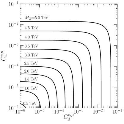
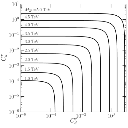
Figure 1: Exclusion contours at $95\%$ C.L. in the $C_{u}^{\ell}$-$C_{d}^{\ell}$ plane for different values of $M_{Z^{\prime}}$, derived using ATLAS data for dilepton final states [52, 53]. In the left panel the contours are for the $\ell\equiv e,\mu$ final state, and the right panel corresponds to the $\tau^{+}\tau^{-}$ final state. For any given $M_{Z^{\prime}}$, the interior of the corresponding contour is allowed.

To analyze the constraints arising from direct resonant $Z^{\prime}$ production at the LHC, decaying to a pair of charged leptons, we first define the chiral couplings $g_{L}^{f}$ and $g_{R}^{f}$ through:

$$g_{R}^{f}=\frac{g}{2\cos\theta_{w}}(g_{V}^{\prime f}-g_{A}^{\prime f}),\;\;g_{L}^{f}=\frac{g}{2\cos\theta_{w}}(g_{V}^{\prime f}+g_{A}^{\prime f}).$$ (27)

From Eq. (26) we note that the right-handed couplings of the light neutrinos to $Z^{\prime}$, $g_{R}^{\nu}$, are zero. In writing Eq. (27), we have implicitly assumed flavor diagonal couplings for $Z^{\prime}$, but kept open the possibility of flavor nonuniversality. With this, the cross section for resonant production of a $Z^{\prime}$ boson at the LHC and its subsequent decay into a pair of charged leptons can be conveniently expressed as (in the narrow width approximation, for illustration)[34]:

$$\sigma\left(pp\to Z^{\prime}X\to\ell^{+}\ell^{-}X\right)=\frac{\pi}{6s}\sum_{q}C_{q}^{\ell}w_{q}\left(s,M_{Z^{\prime}}^{2}\right)\,,$$ (28)

where the sum is over all the partons. The co-efficients,

$$C_{q}^{\ell}=\left[\left(g_{L}^{q}\right)^{2}+\left(g_{R}^{q}\right)^{2}\right]{\rm BR}\left(Z^{\prime}\to\ell^{+}\ell^{-}\right)$$ (29)

involve the fermionic couplings of $Z^{\prime}$ and hence depend on the details of the fermionic sector of the model under consideration. The functions $w_{q}$, on the other hand, contain all the information about the parton distribution functions (PDFs) and QCD corrections, detailed expressions for which appear in the Appendix. Considering the fact that $w_{u}$ and $w_{d}$ are substantially larger than the $w_{q}$ functions for the other quarks, we can approximate Eq. (28) as follows:

$$\sigma\left(pp\to Z^{\prime}X\to\ell^{+}\ell^{-}X\right)\approx\frac{\pi}{6s}\left[C_{u}^{\ell}w_{u}\left(s,M_{Z^{\prime}}^{2}\right)+C_{d}^{\ell}w_{d}\left(s,M_{Z^{\prime}}^{2}\right)\right]\,.$$ (30)

Direct searches at the LHC put upper limits on the left-hand-side of Eq. (28). The most recent ATLAS limits can be found in [52, 53] where, as expected, the bound for the $\ell^{\pm}\equiv\tau^{\pm}$ case is less stringent than for $\ell^{\pm}\equiv e^{\pm},\mu^{\pm}$. Using the CT14NLO PDF set [63], we evaluate $w_{u}$ and $w_{d}$, and translate the limit on the cross section into a bound in the $C_{u}^{\ell}$-$C_{d}^{\ell}$ plane for different values of $M_{Z^{\prime}}$. The results have been displayed in Fig. 1, where the left panel corresponds to $\ell\equiv e,\mu$, and the right panel corresponds to $\ell\equiv\tau$. For any chosen $M_{Z^{\prime}}$, only the interior of the corresponding contour is allowed. Although the bound arising from the $\tau^{+}\tau^{-}$ final state is substantially weaker compared to that from $e^{+}e^{-},\mu^{+}\mu^{-}$ final state, it may have its own advantage for scenarios where, e.g., the $Z^{\prime}$ dominantly couples to the third generation of fermions[65, 66, 67].

4 Theoretical constraint from unitarity

For $U(1)$ extended models, in the absence of a $Z^{\prime}$, the scattering amplitude for the process $W_{L}^{+}W_{L}^{-}\to W_{L}^{+}W_{L}^{-}$, where $W_{L}^{\pm}$ denotes the longitudinal component of the $W$-boson, will grow as the fourth power of the center of momentum (CoM) energy at the leading order. To put it explicitly, if the $Z^{\prime}$ is too heavy to contribute, then we can write the Feynman amplitude for $W_{L}^{+}W_{L}^{-}\to W_{L}^{+}W_{L}^{-}$ as

$${\mathscr{M}}_{W_{L}^{+}W_{L}^{-}\to W_{L}^{+}W_{L}^{-}}=\frac{g^{2}\cos^{2}\theta_{w}E^{4}}{M_{W}^{4}}\sin^{2}\alpha_{z}\left(-3+6\cos\theta+\cos^{2}\theta\right)+{\mathcal{O}}\left(\frac{E^{2}}{M_{W}^{2}}\right)\,,$$ (31)

where $E$ denotes the CoM energy and $\theta$ is the scattering angle. From Eq. (31), the $l=0$ partial wave amplitude which usually gives the strongest bound, can be extracted as

$$a_{0}=-\frac{8}{3}\frac{g^{2}\cos^{2}\theta_{w}E^{4}}{M_{W}^{4}}\sin^{2}\alpha_{z}\,.$$ (32)

Unitarity restricts the magnitude of $a_{0}$ as $|a_{0}|<8\pi$ which translates into an upper bound for the CoM energy,

$$E<E_{\rm max}=\left[8\pi\times\frac{3\left(M_{Z}^{2}\cos^{2}{\alpha_{z}}+M_{Z^{\prime}}^{2}\sin^{2}\alpha_{z}\right)}{32\sqrt{2}G_{F}\sin^{2}\alpha_{z}}\right]^{\frac{1}{4}}\,,$$ (33)

where $G_{F}$ is the Fermi constant obtained via the relation,

$$g^{2}/M_{W}^{2}=4\sqrt{2}G_{F}\,,$$ (34)

and we have used Eq. (17a) to substitute for $M_{W}^{2}/\cos^{2}\theta_{w}$. Thus, to restore unitarity, effects of the $Z^{\prime}$ must set in before the CoM energy reaches $E_{\rm max}$, i.e., $M_{Z^{\prime}}<E_{\rm max}$ which implies:

$$\frac{M^{4}_{Z^{\prime}}\sin^{2}\alpha_{z}}{\left(M_{Z}^{2}\cos^{2}{\alpha_{z}}+M_{Z^{\prime}}^{2}\sin^{2}\alpha_{z}\right)}<8\pi\times\frac{3}{32\sqrt{2}G_{F}}\,.$$ (35)

To find a physical interpretation for the above bound, we write down the expression for the $Z^{\prime}\to W^{+}W^{-}$ decay width as

$$\Gamma(Z^{\prime}\to W^{+}W^{-})\approx\frac{1}{64\pi}\frac{g^{2}\cos^{2}\theta_{w}\sin^{2}\alpha_{z}}{3}M_{Z^{\prime}}\left(\frac{M_{Z^{\prime}}}{M_{W}}\right)^{4}\,,$$ (36)

which is valid in the limit $M_{Z^{\prime}}\gg M_{W}$ when the longitudinal components of the $W$-bosons dominate[68, 69]. Substituting for $\cos\theta_{w}$ using Eq. (17a), one can easily verify that this partial decay width increases with $\sin\alpha_{z}$ as well as $M_{Z^{\prime}}$. However, the resonance should be narrow enough so that it can be distinguished experimentally from the flat background. In view of this, it may be reasonable to impose a rather conservative limit,

$$\Gamma(Z^{\prime}\to W^{+}W^{-})<M_{Z^{\prime}}\,.$$ (37)

Using Eqs. (17a) and (34) one can check that the above bound can be translated into

$$\frac{M^{4}_{Z^{\prime}}\sin^{2}\alpha_{z}}{\left(M_{Z}^{2}\cos^{2}{\alpha_{z}}+M_{Z^{\prime}}^{2}\sin^{2}\alpha_{z}\right)}<48\pi\times\frac{1}{\sqrt{2}G_{F}}\,,$$ (38)

which is slightly weaker than the unitarity bound in Eq. (35). Therefore, consideration of unitarity implicitly keeps the corresponding partial decay width under control.

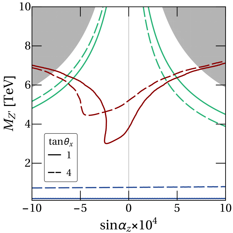
Figure 2: Consolidated bounds in the $(\sin\alpha_{z}$-$M_{Z^{\prime}})$ plane for anomaly-free $U(1)_{X}$ models. The shaded region is excluded from unitarity. The red and the blue colors indicate the limits set by direct detection and $\nu_{\mu}$-$e$ scattering data, respectively. The green contours are obtained by setting $\Gamma_{Z^{\prime}}=M_{Z^{\prime}}/2$. The solid and dashed line-types correspond to $\tan\theta_{x}=1$ and $4$, respectively. Region above the red lines are allowed by the 36 ${\rm fb}^{-1}$ ATLAS data, whereas the region above the blue lines and the interior of the green contours represent the allowed area from the $\nu_{\mu}$-$e$ scattering data and $\Gamma_{Z^{\prime}}\leq M_{Z^{\prime}}/2$, respectively.

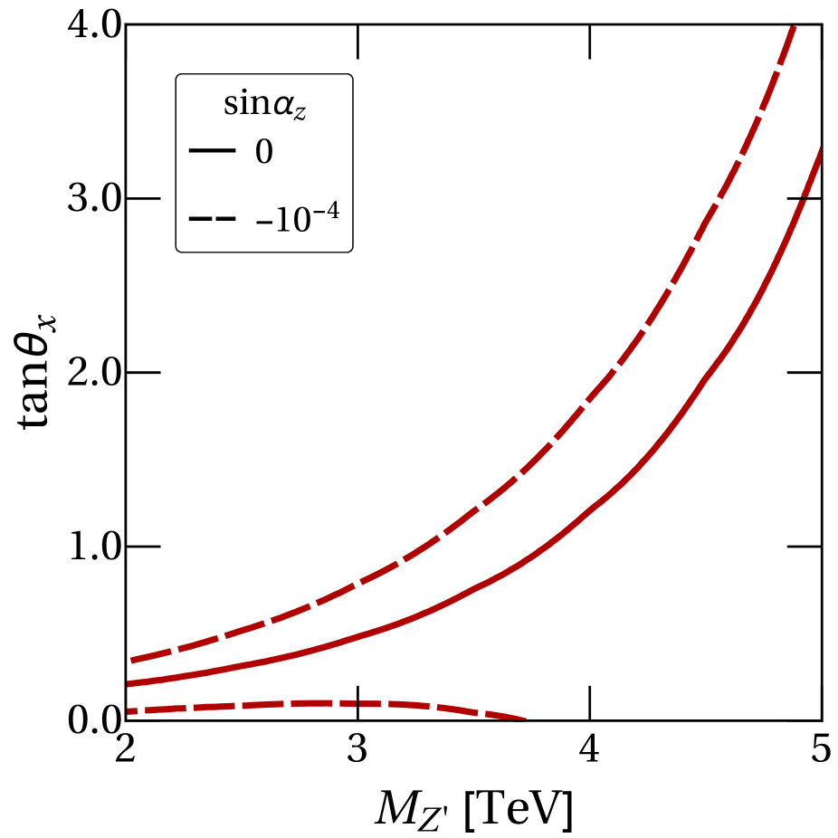
Figure 3: Bounds in the $(M_{Z^{\prime}}$-$\tan\theta_{x})$ plane for anomaly-free $U(1)_{X}$ models using two representative values of $\sin\alpha_{z}$, namely, $0$ and $(-10^{-4})$. For these choices of $\sin\alpha_{z}$ the strongest limits arise from the direct searches, which have been displayed as the red lines. For $\sin\alpha_{z}=0$ the region to the right of the solid red curve is allowed, whereas for $\sin\alpha_{z}=(-10^{-4})$ the allowed region lies within the dashed red curves.

The tree unitarity constraint is of prime importance as it translates to an upper bound on $M_{Z^{\prime}}$, for a given $\sin\alpha_{z}$, complementing the lower bound that comes from direct search experiments. This can be seen from Eq. (35). We show this explicitly when we discuss the interplay of the different bounds in Sec. 6. It should also be noted that although unitarity in the context of $Z^{\prime}$ models have been studied earlier [73, 74], to our knowledge, the possibility of using it to cast an upper bound on the $Z^{\prime}$ mass as in Eq. (35) has not been emphasized before and thus constitutes a new observation in our paper. Moreover, since this analysis does not depend on the details of the fermionic couplings, such a bound is quite general and can be applied to a wide class of $Z^{\prime}$ models.

5 Constraints from $\nu_{\mu}$-$e$ scattering

The unitarity constraint, described in the previous section, relies on sniffing the effects of $Z^{\prime}$ through the $Z$-$Z^{\prime}$ mixing. Therefore, the bounds are lifted in the limit $\sin\alpha_{z}=0$ as has been clearly depicted in Fig. 3. However, depending on how $Z^{\prime}$ couples to the fermions, it is possible to put lower bounds on $M_{Z^{\prime}}$, even in the limit of vanishing $Z$-$Z^{\prime}$ mixing [75, 76]. This can be done, e.g., by using the data from low energy neutrino-electron scattering such as $\nu_{\mu}e\to\nu_{\mu}e$ which proceeds at the tree level purely via neutral current (see, e.g., [77, 74, 78]). In models with an extra $U(1)$, the $Z^{\prime}$ boson will, in general, also contribute to the scattering.

The dimension-six operator governing $\nu_{\mu}$-$e$ scattering at low energies is written as:

$$\mathscr{L}_{\nu e}=-\frac{G_{F}}{\sqrt{2}}\left[\overline{\nu}\gamma^{\mu}\left(1-\gamma^{5}\right)\nu\right]\left[\overline{e}\gamma_{\mu}\left(g_{V}^{\nu e}-g_{A}^{\nu e}\gamma^{5}\right)e\right]\,.$$ (39)

We recall that in the SM, the expressions for $g_{V}^{\nu e}$ and $g_{A}^{\nu e}$ are very simple at the tree level and are given by

$$\left(g_{V}^{\nu e}\right)^{\rm SM}\equiv\left(g_{V}^{e}\right)^{\rm SM}=-\frac{1}{2}+2\sin^{2}\theta_{w}\,,\qquad\left(g_{A}^{\nu e}\right)^{\rm SM}\equiv\left(g_{A}^{e}\right)^{\rm SM}=-\frac{1}{2}\,.$$ (40)

Of course, in the $Z^{\prime}$ models under consideration, the above expressions will be modified (see Eq. (26)) as follows:

$$\left(g_{(V,A)}^{\nu e}\right)^{\rm model} = M_{11}^{2}\left(\frac{\kappa_{Z}g_{(V,A)}^{e}}{M_{Z}^{2}}+\frac{\kappa_{Z^{\prime}}g_{(V,A)}^{\prime e}}{M_{Z^{\prime}}^{2}}\right)\,,$$ (41)

where the expression for $M_{11}^{2}$ appears in Eq. (17a) and the rest of the couplings in Eq. (22).

We use this formula along with the following global fit values from PDG [79]:

$$g_{V}^{\nu e}=-0.040\pm 0.015\,,\qquad g_{A}^{\nu e}=-0.507\pm 0.014\,,$$ (42)

to draw the $2\sigma$ allowed regions in the $\sin\alpha_{z}$-$M_{Z^{\prime}}$ plane for two different values of $\tan\theta_{x}$ as shown by the blue curves in Fig. 3.

6 Results and discussions

Till now we have developed a general formalism on how to constrain a minimal $Z^{\prime}$ model from theoretical considerations as well as from different types of experimental data. Now we combine the different limits together, described in the previous sections, to obtain stronger bounds on the parameter space. To illustrate, $C_{u,d}^{e,\mu}$ and $g_{V}^{\nu e}$ can be determined, using Eqs. (29), (27) and (41) in conjunction with Eq. (22), in terms of the three quantities $M_{Z^{\prime}}$, $\alpha_{z}$ and $\tan\theta_{x}$. The bound from the left panel of Fig. 1 and the constraint coming from $\nu_{\mu}$-$e$ scattering can then be translated to the limits on those three parameters.

In Fig. 3 these bounds have been displayed in the $\sin\alpha_{z}$-$M_{Z^{\prime}}$ plane for any anomaly-free $U(1)_{X}$ model for two typical choices of $\tan\theta_{x}$. The region excluded from unitarity has been shaded in gray and is independent of $\tan\theta_{x}$. The lower bounds on $M_{Z^{\prime}}$, arising from the ATLAS (13 TeV, 36 ${\rm fb}^{-1}$) exclusion of the DY production of $Z^{\prime}$, are depicted as red curves, whereas the region above the light blue curves denote the region consistent with $\nu_{\mu}$-$e$ scattering. Additionally, we also give contours that represent a constraint on the $Z^{\prime}$ decay width, as a guideline for the validity of a particle interpretation. The green lines in the figure arise from the consideration $\Gamma_{Z^{\prime}}\leq M_{Z^{\prime}}/2$.

For all the colored contours, the solid (dashed) curves correspond to $\tan\theta_{x}=1(4)$. Recall that $\tan\theta_{x}$ is proportional to the effective $U(1)_{X}$ coupling, $g^{\prime}_{x}$. As it happens, the lower bounds on $M_{Z^{\prime}}$ arising from low-energy $\nu_{\mu}$-$e$ scattering are considerably weaker than those from direct searches. However, $\nu_{\mu}$-$e$ scattering can put important constraints for hadrophobic $Z^{\prime}$ models when the production of the $Z^{\prime}$ at the LHC is very suppressed. Combining the lower bound on $M_{Z^{\prime}}$ from the direct searches with the corresponding upper bound coming from, e.g., unitarity, we are able to extract an upper limit on the magnitude of the $Z$-$Z^{\prime}$ mixing angle, $\alpha_{z}$. Such bounds on $|\alpha_{z}|$ are at par with the corresponding limits from electroweak precision data [80, 47].

	Maximum $|\sin\alpha_{z}|$	$10^{-3}$
$\tan\theta_{x}=4$	$M_{Z^{\prime}}$ exclusion at $\alpha_{z}=0$ [in TeV]	5.1
	Lowest possible value of $M_{Z^{\prime}}$ [in TeV]	4.4
	Maximum $|\sin\alpha_{z}|$	$10^{-3}$
$\tan\theta_{x}=1$	$M_{Z^{\prime}}$ exclusion at $\alpha_{z}=0$ [in TeV]	3.8
	Lowest possible value of $M_{Z^{\prime}}$ [in TeV]	3.0

Table 4: Summary of bounds on $M_{Z^{\prime}}$ and $\alpha_{z}$ for anomaly-free $U(1)_{X}$ models using two representative values of $\tan\theta_{x}$ (which is proportional to the effective $U(1)_{X}$ coupling).

In Table 4, we have summarized the bounds on $\alpha_{z}$ and $M_{Z^{\prime}}$ for $\tan\theta_{x}$=1 and 4 for anomaly-free $U(1)_{X}$ models. From Table 2 we recall that the choice $\tan\theta_{x}=4$ corresponds to $g^{\prime}_{x}=g$ for the ‘conventional’ $(B-L)$ model. This is so because for $(B-L)$ model in our normalization, $\kappa_{x}=1/4$, and $g^{\prime}_{x}\kappa_{x}$ in our setup is equivalent to a generic $g^{\prime}_{x}$ in the conventional $(B-L)$ model. It should be pointed out that although we have taken into account the decays $Z^{\prime}\to W^{+}W^{-}$ and $Z^{\prime}\to Zh$ ($h$ being the lighter SM-like Higgs scalar) for our analysis, we have assumed the decays $Z^{\prime}\to NN$, where $N$ denotes a heavy RH neutrino, and $Z^{\prime}\to ZH$, where $H$ is the heavier nonstandard scalar, to be kinematically forbidden. The lower bound on $M_{Z^{\prime}}$ is likely to be diluted further if these decay channels open up.

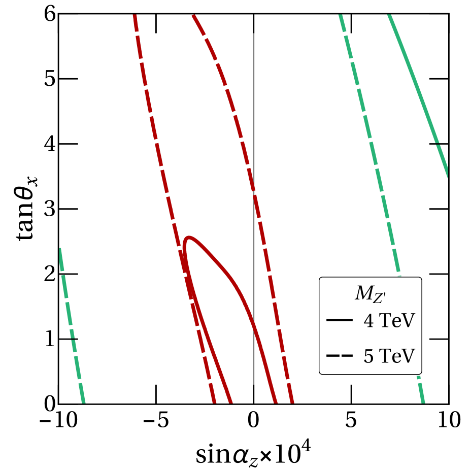
Figure 4: Consolidated bounds in the $(\sin\alpha_{z}$-$\tan\theta_{x})$ plane for anomaly-free $U(1)_{X}$ models using two representative values of $M_{Z^{\prime}}$, namely, $4$ TeV and $5$ TeV. For these values of $M_{Z^{\prime}}$ strongest limits come from direct searches, displayed by the red lines. For $M_{Z^{\prime}}=4$ TeV the region inside the solid red contour is allowed, whereas for $M_{Z^{\prime}}=5$ TeV the region bounded within the dashed red lines is allowed. The green lines refer to $\Gamma_{Z^{\prime}}\leq M_{Z^{\prime}}/2$ for which the limits are rather weak for the chosen values of $M_{Z^{\prime}}$ (region inside the dashed lines are allowed for $M_{Z^{\prime}}=5$ TeV, while for $M_{Z^{\prime}}=4$ TeV only one side of the contour, the solid line, is visible).

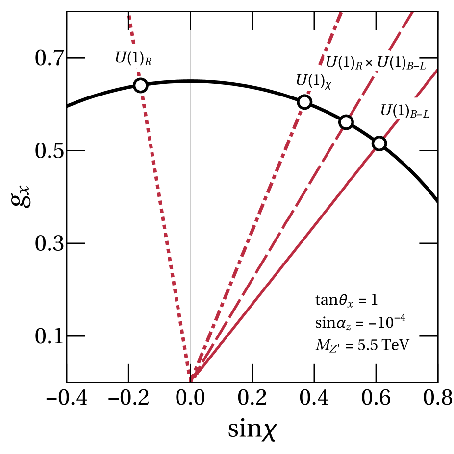
Figure 5: Example plot illustrating the inter-relationship between kinetic mixing ($\sin\chi$) and the original $U(1)_{X}$ coupling ($g_{x}$) assuming hypothetical measurements: $M_{Z^{\prime}}\approx 5.5$ TeV, $\sin\alpha_{z}\approx(-10^{-4})$ and $\tan\theta_{x}\approx 1$. The solid black curve is the contour corresponding to Eq. (9c). Each red line corresponds to a particular model, drawn in conformity with Eqs. (9d) and (17c). The intersection of the black curve with a particular red line gives the solutions for the kinetic mixing and $g_{x}$ for a given model.

It may be useful to note that every point in the $\sin\alpha_{z}$-$M_{Z^{\prime}}$ plane in Fig. 3 corresponds, through Eq. (25), to a definite value of ${\cal F}$. If a specific model is chosen then one can use the relation

$$\tan\chi=\left(2\kappa_{x}-\frac{1}{2}\right)\tan\theta_{x}\cot\theta_{w}-\frac{{\cal F}}{\sin\theta_{w}}\,,$$ (43)

which follows from Eq. (17c), to determine the kinetic mixing angle, $\chi$, corresponding to this point. The value of $\kappa_{x}$ varies from model to model, $\tan\theta_{x}$ is a measure of the effective gauge coupling of the extra $U(1)_{X}$, and $\cos\theta_{w}$ is determined in terms of $\sin\alpha_{z}$ and $M_{Z^{\prime}}$ through Eq. (17a). Conversely, for a fixed value of the kinetic mixing parameter, $\chi$, any model would correspond to a curve, determined by $\kappa_{x}$, in the $\sin\alpha_{z}$-$M_{Z^{\prime}}$ plane. As a definite example, if we consider the $(B-L)$ model ($\kappa_{x}=1/4$), the curve corresponding to $\chi=0$ is a vertical straight line through the origin. This is reminiscent of the fact that in this model $Z$-$Z^{\prime}$ mixing is entirely due to kinetic mixing.

In Fig. 3, we take a complementary approach by casting the bounds in the $M_{Z^{\prime}}$-$\tan\theta_{x}$ plane, for two representative values of $\sin\alpha_{z}$, namely, $0$ and $(-10^{-4})$. For these values of $\sin\alpha_{z}$ strongest limits come from direct searches, which have been displayed by the red lines. For $\sin\alpha_{z}=0$ the region to the right of the solid red line is allowed, whereas for $\sin\alpha_{z}=(-10^{-4})$ the region contained within the dashed red lines is allowed. The absence of contours from considerations of unitarity and $\nu_{\mu}$-$e$ scattering in Fig. 3 implies that the corresponding curves are too weak to enter inside the zoomed range of the parameter space.

In Fig. 5, we display the bounds in the $\sin\alpha_{z}$-$\tan\theta_{x}$ plane, for two representative values of $M_{Z^{\prime}}$, namely, $4$ TeV and $5$ TeV. For these values of $M_{Z^{\prime}}$ strongest limits come from direct searches, displayed by the red lines. For $M_{Z^{\prime}}=4$ TeV the region inside the solid red contour is allowed, whereas for $M_{Z^{\prime}}=5$ TeV the region bounded within the dashed red lines is allowed. The green lines correspond to $\Gamma_{Z^{\prime}}\leq M_{Z^{\prime}}/2$.

Finally, with the ambitious expectation that a $Z^{\prime}$ will be discovered in future, in Fig. 5 we illustrate how model specific information can be extracted using the following hypothetical measurements of the model-independent parameters:

$$M_{Z^{\prime}}\approx 5.5\,{\rm TeV}\,,\qquad\sin\alpha_{z}\approx(-10^{-4})\,,\qquad\tan\theta_{x}\approx 1\,.$$ (44)

The solid black line in Fig. 5 has been obtained by combining Eqs. (9b) and (9c) for $\tan\theta_{x}=1$. It does not depend on the chosen model. The red lines, on the other hand, are drawn using Eq. (9d) in conjunction with Eqs. (17a) and (17c) to trade $\theta_{w}$ and $x^{\prime}_{\Phi}$ in favor of $M_{Z^{\prime}}$, $\alpha_{z}$ and $\tan\theta_{x}$. Since the red lines require the input of $x_{\Phi}$ which, in turn, depends on $\kappa_{x}$, the lines are different for different models. The intersection of the black line with a particular red line gives the solutions for the kinetic mixing parameter, $\chi$, and the $U(1)_{X}$ coupling, $g_{x}$, for that particular model. Such a solution might provide intuition as to whether a specific $U(1)_{X}$ model fits into a more elaborate scheme, such as grand unification, at higher energies.

7 Conclusions

Our intention in this paper has been to put constraints on the parameter space of the minimal extension of the SM with an additional gauged $U(1)$ giving a massive neutral $Z^{\prime}$ gauge boson. We did revisit the formalism first to set up the notations. We have advocated a parametrization in which, in the presence of kinetic mixing, the constraints on different anomaly-free $U(1)_{X}$ models can be expressed in a model-independent unified framework. Importantly, we have not a priori assumed, unlike most of the previous works, that the $Z$-$Z^{\prime}$ mixing angle is small or the $Z^{\prime}$ mass is way above the $Z$ mass. For the sake of illustration we explicitly examine a few popular scenarios of $U(1)$ extension, e.g., the $(B-L)$ model, an $U(1)$ arising from left-right symmetry, etc. It turns out that there are three important quantities to be determined which cover the extended parameter space and absorb all model dependence for a non-anomalous $U(1)$ extension. These quantities are the mass of the $Z^{\prime}$, the effective gauge coupling strength ($g^{\prime}_{x}$) of the extra $U(1)$, and the $Z$-$Z^{\prime}$ mixing angle ($\alpha_{z}$). To constrain this space, we have primarily employed three types of information, namely, the LHC (ATLAS) 13 TeV Drell-Yan data with 36 ${\rm fb}^{-1}$ luminosity, the results from low energy $\nu_{\mu}-e$ scattering, and consistency with $s$-wave unitarity in the $W_{L}^{+}W_{L}^{-}\to W_{L}^{+}W_{L}^{-}$ channel. The LHC data turn out to be most constraining. We also observe that constraints on the $Z^{\prime}$ decay width, $\Gamma_{Z^{\prime}}$, translate to constraints in the parameter space which are similar in nature to those obtained from $s$-wave unitarity. We want to underscore that although we employ the anomaly-free (per generation) models to exemplify our formalism, the analysis can in general be used to constrain other extensions of the SM with an additional $Z^{\prime}$. The interplay between the different bounds can be used to constrain models with or without couplings to fermions, and with or without $Z$-$Z^{\prime}$ mixing. Also, models with a $Z^{\prime}$ that couples only to leptons, or even preferentially to the third generation can be constrained using our study. The new things that emerge from our analysis are the following:

• Our parametrization shows that increasingly precise experimental data would squeeze the allowed region in the three-dimensional space of $M_{Z^{\prime}}$, $\alpha_{z}$ and $\theta_{x}$. The description is completely model-independent as long as the fermion content ensures an anomaly-free set-up. Model dependence is encoded in $\kappa_{x}$, which is different for different models, as listed in Table 2. Of the other parameters, the strength of kinetic mixing, $\chi$, should in principle be a derived quantity in a fundamental theory given the charges of a possible set of heavy particles (couplings both to $B_{\mu}$ and $X_{\mu}$), integrated out to generate the mixing. Nevertheless, in our approach, which is agnostic towards models of UV completion, $\chi$ is treated as an effective parameter. Given a model (i.e. a value of $\kappa_{x}$), one can calculate a range in $\chi$ using Eq. (43) which would fit values (or limits) of $M_{Z^{\prime}}$, $\alpha_{z}$ and $\theta_{x}$ extracted directly from experimental data.

• We have updated the model-independent constraints in the $C_{u}^{\ell}$-$C_{d}^{\ell}$ ($\ell\equiv e,\mu$) plane, using the latest 13 TeV (36 ${\rm fb}^{-1}$) ATLAS data. We obtain an improvement of one order of magnitude over the previous constraints in the same plane obtained from the publicly available 7-8 TeV CMS results [64] (see also [37]), and several orders of magnitude over those from Tevatron results [34]. While constraints were speculated before actual LHC data arrived [10, 35, 36], our analysis provides the most updated ones in the $C_{u}^{\ell}$-$C_{d}^{\ell}$ plane using the latest publicly available LHC (ATLAS) data. Translating experimental data to constraints in the above plane as a function of $(M_{Z^{\prime}},C_{u}^{\ell},C_{d}^{\ell})$, rather than directly to limits on $M_{Z^{\prime}}/g^{{}^{\prime}2}_{x}$, is quite useful as it provides a model-independent platform from where limits on any type of specific customized models can be easily extracted. ATLAS has also provided bounds for Drell-Yan $\tau^{+}\tau^{-}$ production through a $Z^{\prime}$. We use this dataset to set similar constraints in the $C_{u}^{\tau}$-$C_{d}^{\tau}$ plane. Though less restrictive, these latter bounds are useful for non-universal $Z^{\prime}$ models which have a different coupling to the third generation fermions.

• The $s$-wave unitarity constraints in the ($M_{Z^{\prime}}$-$\sin\alpha_{z}$) plane, placed for the first time in this paper, turn out to provide complementary limits when the LHC direct search and the low energy $\nu_{\mu}$-$e$ scattering constraints are superposed in the same plane. It is important to observe that the unitarity constraints are insensitive to the extra $U(1)$ coupling strength, $g^{\prime}_{x}$, and in conjunction with the LHC direct search limits they restrict the $Z$-$Z^{\prime}$ mixing to be small (which we have not a priori assumed). However, when we require $\Gamma_{Z^{\prime}}\leq 0.5~{}M_{Z^{\prime}}$, the constrained turn out to be much stronger than the ones obtained from $\nu_{\mu}$-$e$ scattering data or from satisfying $s$-wave unitarity. The constraints on the mixing angle ($\alpha_{z}$) we obtain are, in fact, of the same order as obtained from electroweak precision tests [80, 47].

• When the $Z^{\prime}$ couples to fermions with the same strength as that of the SM $SU(2)_{L}$ gauge boson (for $(B-L)$ model this corresponds to $\tan\theta_{x}=4$), we obtain $M_{Z^{\prime}}>4.4$ TeV and $|\alpha_{z}|<0.001$ at $95\%$ C.L.

We urge our experimental colleagues to take notice of our assertion that a model independent analysis, as depicted especially by the direct detection contour in Fig. 3, can be carried out with just three independent parameters, as discussed in detail.

Note added :

While this manuscript was being finalized, the 13 TeV Drell-Yan data from the CMS Collaboration became available[81]. Our result in the $C_{u}^{e,\mu}$-$C_{d}^{e,\mu}$ plane, which uses the 13 TeV ATLAS Drell-Yan data, is very similar to that obtained by the CMS collaboration. Analysis using the 13 TeV ATLAS Drell-Yan data has also been performed very recently in Refs. [82, 83].

Acknowledgements :

TB acknowledges a Senior Research Fellowship from UGC, India. GB and AR acknowledge support of the J.C. Bose National Fellowship from the Department of Science and Technology, Government of India (SERB Grant Nos. SB/S2/JCB-062/2016 and SR/S2/JCB-14/2009, respectively). AR also acknowledges suport from the SERB Grant No. EMR/2015/001989.

Appendix: Detailed expressions for $w_{q}$

The NLO expressions for the functions, $w_{q}$, which appear in Eq. (28), are given by

$$w_{q}\left(s,M_{Z^{\prime}}^{2}\right) = \int_{0}^{1}dx\int_{0}^{1}dy\int_{0}^{1}dz\,\,\delta\left(\frac{M_{Z^{\prime}}^{2}}{s}-xyz\right)\times$$ (A.1)

$$\Big{\{}F_{qq}\left(x,y,M_{Z^{\prime}}^{2}\right)\Delta_{qq}\left(z,M_{Z^{\prime}}^{2}\right)+F_{gq}\left(x,y,M_{Z^{\prime}}^{2}\right)\Delta_{gq}\left(z,M_{Z^{\prime}}^{2}\right)\Big{\}}\,,$$

For $pp$ colliders such as the LHC we have[34]:

$$F_{qq}\left(x,y,M_{Z^{\prime}}^{2}\right) = f_{q\leftarrow P}\left(x,M_{Z^{\prime}}^{2}\right)f_{\overline{q}\leftarrow{P}}\left(y,M_{Z^{\prime}}^{2}\right)+\left(x\leftrightarrow y\right)\,,$$ (A.2a)

$$F_{gq}\left(x,y,M_{Z^{\prime}}^{2}\right) = f_{g\leftarrow P}\left(x,M_{Z^{\prime}}^{2}\right)\left[f_{q\leftarrow{P}}\left(y,M_{Z^{\prime}}^{2}\right)+f_{\overline{q}\leftarrow{P}}\left(y,M_{Z^{\prime}}^{2}\right)\right]+\left(x\leftrightarrow y\right)\,,$$ (A.2b)

where $f_{q\leftarrow P}\left(x,M_{Z^{\prime}}^{2}\right)$ represents the PDF for the parton $q$ at a factorization scale, $M_{Z^{\prime}}$. The scaling functions, $\Delta_{qq}$ and $\Delta_{gq}$, are given by[84]

$$\Delta_{qq}\left(z,M_{Z^{\prime}}^{2}\right) = \delta(1-z)+\frac{\alpha_{s}(M_{Z^{\prime}}^{2})}{\pi}C_{F}\left[\left(\frac{\pi^{2}}{3}-4\right)\delta(1-z)-\frac{1+z^{2}}{1-z}\ln(z)\right.$$ (A.3a)

$$\left.-2(1+z)\ln(1-z)+4(1+z^{2})\left(\frac{\ln(1-z)}{1-z}\right)_{+}\right]\,,$$

$$\Delta_{gq}\left(z,M_{Z^{\prime}}^{2}\right) = \frac{\alpha_{s}(M_{Z^{\prime}}^{2})}{2\pi}T_{F}\left[(1-2z+2z^{2})\ln\frac{(1-z)^{2}}{z}+\frac{1}{2}+3z-\frac{7}{2}z^{2}\right]\,,$$ (A.3b)

where $C_{F}=4/3$ and $T_{F}=1/2$ are the quark and gluon color factors respectively. The plus prescription is defined as follows:

$$\int_{0}^{1}dx\,\,f(x)\,g(x)_{+}=\int_{0}^{1}dx\left[f(x)-f(1)\right]\,g(x)\,.$$ (A.4)

We obtained our numerical results using these equations.

References

- [1] J. C. Pati and A. Salam, Is Baryon Number Conserved?, Phys. Rev. Lett. 31 (1973) 661–664.
- [2] J. C. Pati and A. Salam, Lepton Number as the Fourth Color, Phys. Rev. D10 (1974) 275–289. [Erratum: Phys. Rev. D11, 703 (1975)].
- [3] R. N. Mohapatra and J. C. Pati, “Natural” left-right symmetry, Phys. Rev. D11 (1975) 2558–2561.
- [4] G. Senjanovic and R. N. Mohapatra, Exact Left-Right Symmetry and Spontaneous Violation of Parity, Phys. Rev. D12 (1975) 1502–1505.
- [5] H. Georgi, The State of the Art Gauge Theories, AIP Conf.Proc. 23 (1975) 575–582.
- [6] H. Fritzsch and P. Minkowski, Unified Interactions of Leptons and Hadrons, Annals Phys. 93 (1975) 193–266.
- [7] F. Gursey, P. Ramond, and P. Sikivie, A Universal Gauge Theory Model Based on E6, Phys. Lett. 60B (1976) 177–180.
- [8] D. London and J. L. Rosner, Extra Gauge Bosons in E(6), Phys. Rev. D34 (1986) 1530.
- [9] P. Langacker, Grand Unified Theories and Proton Decay, Phys. Rept. 72 (1981) 185.
- [10] T. G. Rizzo, phenomenology and the LHC, in Proceedings of Theoretical Advanced Study Institute in Elementary Particle Physics : Exploring New Frontiers Using Colliders and Neutrinos (TASI 2006): Boulder, Colorado, June 4-30, 2006, pp. 537–575, 2006. hep-ph/0610104.
- [11] J. L. Hewett and T. G. Rizzo, Low-Energy Phenomenology of Superstring Inspired E(6) Models, Phys. Rept. 183 (1989) 193.
- [12] M. Cvetic and P. Langacker, Implications of Abelian extended gauge structures from string models, Phys. Rev. D54 (1996) 3570–3579, [hep-ph/9511378].
- [13] A. Leike, The Phenomenology of extra neutral gauge bosons, Phys. Rept. 317 (1999) 143–250, [hep-ph/9805494].
- [14] P. Langacker, The Physics of Heavy Gauge Bosons, Rev. Mod. Phys. 81 (2009) 1199–1228, [arXiv:0801.1345].
- [15] N. Arkani-Hamed, A. G. Cohen, and H. Georgi, Electroweak symmetry breaking from dimensional deconstruction, Phys. Lett. B513 (2001) 232–240, [hep-ph/0105239].
- [16] M. Perelstein, Little Higgs models and their phenomenology, Prog. Part. Nucl. Phys. 58 (2007) 247–291, [hep-ph/0512128].
- [17] Y. Shadmi and Y. Shirman, Dynamical supersymmetry breaking, Rev. Mod. Phys. 72 (2000) 25–64, [hep-th/9907225].
- [18] I. Antoniadis, A Possible new dimension at a few TeV, Phys. Lett. B246 (1990) 377–384.
- [19] T. Appelquist, H.-C. Cheng, and B. A. Dobrescu, Bounds on universal extra dimensions, Phys. Rev. D64 (2001) 035002, [hep-ph/0012100].
- [20] K. Agashe, A. Delgado, M. J. May, and R. Sundrum, RS1, custodial isospin and precision tests, JHEP 08 (2003) 050, [hep-ph/0308036].
- [21] S. Iso, N. Okada, and Y. Orikasa, The minimal B-L model naturally realized at TeV scale, Phys. Rev. D80 (2009) 115007, [arXiv:0909.0128].
- [22] S. Oda, N. Okada, D. Raut, and D.-s. Takahashi, Non-minimal quartic inflation in classically conformal U(1)X extended Standard Model, arXiv:1711.09850.
- [23] A. Achucarro and T. Vachaspati, Semilocal and electroweak strings, Phys. Rept. 327 (2000) 347–426, [hep-ph/9904229]. [Phys. Rept.327,427(2000)].
- [24] E. Dudas, Y. Mambrini, S. Pokorski, and A. Romagnoni, (In)visible Z-prime and dark matter, JHEP 08 (2009) 014, [arXiv:0904.1745].
- [25] E. Dudas, Y. Mambrini, S. Pokorski, and A. Romagnoni, Extra U(1) as natural source of a monochromatic gamma ray line, JHEP 10 (2012) 123, [arXiv:1205.1520].
- [26] R. Foot and S. Vagnozzi, Dissipative hidden sector dark matter, Phys. Rev. D91 (2015) 023512, [arXiv:1409.7174].
- [27] R. Foot and S. Vagnozzi, Diurnal modulation signal from dissipative hidden sector dark matter, Phys. Lett. B748 (2015) 61–66, [arXiv:1412.0762].
- [28] N. Okada and S. Okada, -portal right-handed neutrino dark matter in the minimal U(1)X extended Standard Model, Phys. Rev. D95 (2017), no. 3 035025, [arXiv:1611.02672].
- [29] N. Okada, S. Okada, and D. Raut, SU(5)U(1)X grand unification with minimal seesaw and -portal dark matter, Phys. Lett. B780 (2018) 422–426, [arXiv:1712.05290].
- [30] S. Okada, portal dark matter in the minimal model, arXiv:1803.06793.
- [31] B. Kors and P. Nath, A Stueckelberg extension of the standard model, Phys. Lett. B586 (2004) 366–372, [hep-ph/0402047].
- [32] A. Berlin, D. Hooper, and S. D. McDermott, Simplified Dark Matter Models for the Galactic Center Gamma-Ray Excess, Phys. Rev. D89 (2014), no. 11 115022, [arXiv:1404.0022].
- [33] J. M. Cline, G. Dupuis, Z. Liu, and W. Xue, The windows for kinetically mixed Z’-mediated dark matter and the galactic center gamma ray excess, JHEP 08 (2014) 131, [arXiv:1405.7691].
- [34] M. Carena, A. Daleo, B. A. Dobrescu, and T. M. P. Tait, gauge bosons at the Tevatron, Phys. Rev. D70 (2004) 093009, [hep-ph/0408098].
- [35] F. Petriello and S. Quackenbush, Measuring couplings at the CERN LHC, Phys. Rev. D77 (2008) 115004, [arXiv:0801.4389].
- [36] E. Salvioni, G. Villadoro, and F. Zwirner, Minimal Z-prime models: Present bounds and early LHC reach, JHEP 11 (2009) 068, [arXiv:0909.1320].
- [37] E. Accomando, A. Belyaev, L. Fedeli, S. F. King, and C. Shepherd-Themistocleous, Z’ physics with early LHC data, Phys. Rev. D83 (2011) 075012, [arXiv:1010.6058].
- [38] M. R. Buckley, D. Hooper, J. Kopp, and E. Neil, Light Z’ Bosons at the Tevatron, Phys. Rev. D83 (2011) 115013, [arXiv:1103.6035].
- [39] E. Accomando, C. Coriano, L. Delle Rose, J. Fiaschi, C. Marzo, and S. Moretti, , Higgses and heavy neutrinos in models: from the LHC to the GUT scale, JHEP 07 (2016) 086, [arXiv:1605.02910].
- [40] N. Okada and S. Okada, portal dark matter and LHC Run-2 results, Phys. Rev. D93 (2016), no. 7 075003, [arXiv:1601.07526].
- [41] A. De Simone, G. F. Giudice, and A. Strumia, Benchmarks for Dark Matter Searches at the LHC, JHEP 06 (2014) 081, [arXiv:1402.6287].
- [42] O. Buchmueller, M. J. Dolan, S. A. Malik, and C. McCabe, Characterising dark matter searches at colliders and direct detection experiments: Vector mediators, JHEP 01 (2015) 037, [arXiv:1407.8257].
- [43] O. Ducu, L. Heurtier, and J. Maurer, LHC signatures of a Z’ mediator between dark matter and the SU(3) sector, JHEP 03 (2016) 006, [arXiv:1509.05615].
- [44] M. Klasen, F. Lyonnet, and F. S. Queiroz, NLO+NLL collider bounds, Dirac fermion and scalar dark matter in the B–L model, Eur. Phys. J. C77 (2017), no. 5 348, [arXiv:1607.06468].
- [45] R. Gauld, F. Goertz, and U. Haisch, On minimal explanations of the anomaly, Phys. Rev. D89 (2014) 015005, [arXiv:1308.1959].
- [46] A. J. Buras and J. Girrbach, Left-handed and FCNC quark couplings facing new data, JHEP 12 (2013) 009, [arXiv:1309.2466].
- [47] J. Erler, P. Langacker, S. Munir, and E. Rojas, Improved Constraints on Z-prime Bosons from Electroweak Precision Data, JHEP 08 (2009) 017, [arXiv:0906.2435].
- [48] G. Bhattacharyya, A. Datta, S. N. Ganguli, and A. Raychaudhuri, Z - Z-prime mixing in extended gauge models from LEP 1990 data, Mod. Phys. Lett. A6 (1991) 2557–2568.
- [49] G. Bhattacharyya, A. Raychaudhuri, A. Datta, and S. N. Ganguli, DECAY CONFRONTS NONSTANDARD SCENARIOS, Phys. Rev. Lett. 64 (1990) 2870–2873.
- [50] R. H. Benavides, L. Muñoz, W. A. Ponce, O. Rodríguez, and E. Rojas, Electroweak couplings and LHC constraints on alternative models in , arXiv:1801.10595.
- [51] A. Ekstedt, R. Enberg, G. Ingelman, J. Löfgren, and T. Mandal, Constraining minimal anomaly free extensions of the Standard Model, JHEP 11 (2016) 071, [arXiv:1605.04855].
- [52] ATLAS Collaboration, M. Aaboud et al., Search for new high-mass phenomena in the dilepton final state using 36 fb-1 of proton-proton collision data at TeV with the ATLAS detector, JHEP 10 (2017) 182, [arXiv:1707.02424].
- [53] ATLAS Collaboration, M. Aaboud et al., Search for additional heavy neutral Higgs and gauge bosons in the ditau final state produced in 36 fb-1 of pp collisions at TeV with the ATLAS detector, JHEP 01 (2018) 055, [arXiv:1709.07242].
- [54] B. Holdom, Two U(1)’s and Epsilon Charge Shifts, Phys. Lett. 166B (1986) 196–198.
- [55] K. S. Babu, C. F. Kolda, and J. March-Russell, Implications of generalized Z - Z-prime mixing, Phys. Rev. D57 (1998) 6788–6792, [hep-ph/9710441].
- [56] B. Brahmachari and A. Raychaudhuri, Perturbative generation of from tribimaximal neutrino mixing, Phys. Rev. D86 (2012) 051302, [arXiv:1204.5619].
- [57] K. S. Babu, C. F. Kolda, and J. March-Russell, Leptophobic U(1) and the R() - R() crisis, Phys. Rev. D54 (1996) 4635–4647, [hep-ph/9603212].
- [58] C.-W. Chiang, T. Nomura, and K. Yagyu, Phenomenology of -Inspired Leptophobic Boson at the LHC, JHEP 05 (2014) 106, [arXiv:1402.5579].
- [59] J. Y. Araz, G. Corcella, M. Frank, and B. Fuks, Loopholes in searches at the LHC: exploring supersymmetric and leptophobic scenarios, JHEP 02 (2018) 092, [arXiv:1711.06302].
- [60] D. Feldman, Z. Liu, and P. Nath, The Stueckelberg Prime at the LHC: Discovery Potential, Signature Spaces and Model Discrimination, JHEP 11 (2006) 007, [hep-ph/0606294].
- [61] G. Paz and J. Roy, A comment on the Z’ Drell-Yan cross section, arXiv:1711.02655.
- [62] A. A. Andrianov, P. Osland, A. A. Pankov, N. V. Romanenko, and J. Sirkka, On the phenomenology of a coupling only to third family fermions, Phys. Rev. D58 (1998) 075001, [hep-ph/9804389].
- [63] S. Dulat, T.-J. Hou, J. Gao, M. Guzzi, J. Huston, P. Nadolsky, J. Pumplin, C. Schmidt, D. Stump, and C. P. Yuan, New parton distribution functions from a global analysis of quantum chromodynamics, Phys. Rev. D93 (2016), no. 3 033006, [arXiv:1506.07443].
- [64] CMS Collaboration, V. Khachatryan et al., Search for physics beyond the standard model in dilepton mass spectra in proton-proton collisions at TeV, JHEP 04 (2015) 025, [arXiv:1412.6302].
- [65] D. J. Muller and S. Nandi, Top flavor: A Separate SU(2) for the third family, Phys. Lett. B383 (1996) 345–350, [hep-ph/9602390].
- [66] K. R. Lynch, E. H. Simmons, M. Narain, and S. Mrenna, Finding bosons coupled preferentially to the third family at LEP and the Tevatron, Phys. Rev. D63 (2001) 035006, [hep-ph/0007286].
- [67] R. Benavides, L. A. Muñoz, W. A. Ponce, O. Rodríguez, and E. Rojas, Minimal nonuniversal electroweak extensions of the standard model: A chiral multiparameter solution, Phys. Rev. D95 (2017), no. 11 115018, [arXiv:1612.07660].
- [68] F. del Aguila, M. Quiros, and F. Zwirner, On the Mass and the Signature of a New , Nucl. Phys. B284 (1987) 530–556.
- [69] N. G. Deshpande and J. Trampetic, Decay of in and Higgs Modes, Phys. Lett. B206 (1988) 665–668.
- [70] J. F. Gunion, H. E. Haber, G. L. Kane, and S. Dawson, The Higgs Hunter’s Guide, Front. Phys. 80 (2000) 1–404.
- [71] G. Bhattacharyya, D. Das, and P. B. Pal, Modified Higgs couplings and unitarity violation, Phys. Rev. D87 (2013) 011702, [arXiv:1212.4651].
- [72] K. S. Babu, J. Julio, and Y. Zhang, Perturbative unitarity constraints on general W’ models and collider implications, Nucl. Phys. B858 (2012) 468–487, [arXiv:1111.5021].
- [73] K. Cheung, C.-W. Chiang, Y.-K. Hsiao, and T.-C. Yuan, Longitudinal Weak Gauge Bosons Scattering in Hidden Z-prime Models, Phys. Rev. D81 (2010) 053001, [arXiv:0911.0734].
- [74] G. Radel and R. Beyer, Neutrino electron scattering, Mod. Phys. Lett. A8 (1993) 1067–1088.
- [75] M. Lindner, F. S. Queiroz, W. Rodejohann, and X.-J. Xu, Neutrino-Electron Scattering: General Constraints on Z’ and Dark Photon Models, arXiv:1803.00060.
- [76] M. Abdullah, J. B. Dent, B. Dutta, G. L. Kane, S. Liao, and L. E. Strigari, Coherent Elastic Neutrino Nucleus Scattering (CENS) as a probe of through kinetic and mass mixing effects, arXiv:1803.01224.
- [77] F. J. Hasert et al., Search for Elastic Electron Scattering, Phys. Lett. B46 (1973) 121–124. [,5.11(1973)].
- [78] M. Williams, C. P. Burgess, A. Maharana, and F. Quevedo, New Constraints (and Motivations) for Abelian Gauge Bosons in the MeV-TeV Mass Range, JHEP 08 (2011) 106, [arXiv:1103.4556].
- [79] Particle Data Group Collaboration, C. Patrignani et al., Review of Particle Physics, Chin. Phys. C40 (2016), no. 10 100001.
- [80] M. Czakon, J. Gluza, F. Jegerlehner, and M. Zralek, Confronting electroweak precision measurements with new physics models, Eur. Phys. J. C13 (2000) 275–281, [hep-ph/9909242].
- [81] CMS Collaboration, A. M. Sirunyan et al., Search for high-mass resonances in dilepton final states in proton-proton collisions at 13 TeV, arXiv:1803.06292.
- [82] A. Gulov, A. Pankov, A. Pevzner, and V. Skalozub, Model-independent constraints on the Abelian couplings within the ATLAS data on the dilepton production processes at 13 TeV, arXiv:1803.07532.
- [83] A. Pevzner, Influence of the mixing on the production cross section in the model-independent approach, arXiv:1803.07508.
- [84] R. Hamberg, W. L. van Neerven, and T. Matsuura, A complete calculation of the order correction to the Drell-Yan factor, Nucl. Phys. B359 (1991) 343–405. [Erratum: Nucl. Phys.B644,403(2002)].