Direct computational approach to lattice supersymmetric quantum mechanics

Abstract

We propose a numerical method of estimating various physical quantities in lattice (supersymmetric) quantum mechanics. The method consists only of deterministic processes such as computing a product of transfer matrix, and has no statistical uncertainties. We use the numerical quadrature to define the transfer matrix as a finite dimensional matrix, and find that it effectively works by rescaling variable for sufficiently small lattice spacings. For a lattice supersymmetric quantum mechanics, the correlators can be estimated without statistical errors, and the effective masses coincide with the exact solution within very small errors less than $0.001$%. The SUSY Ward identity is also precisely studied in compared with the Monte-Carlo method. Our method is not limited to a lattice SUSY quantum mechanics, but is also applicable to any other lattice models of quantum mechanics.

1 Introduction

Supersymmetric quantum mechanics (SUSY QM) has been extensively studied since it provides a good testing ground for supersymmetric field theories Witten:1981nf ; Witten:1982df ; Cooper:1994eh . Supersymmetry breaking triggered by instantons has been deeply understood and the associated topological index (Witten index) are widely used in other theories. In early studies, a class of exactly solvable potentials, so-called shape invariant potentials (SIP), was discovered and has attracted much attentions in revealing various aspects of SUSY QM Gendenshtein:1984vs . However, to learn SUSY models beyond those cases, numerical approaches including lattice theory could play a significant role.

There have been many attempts to define SUSY QM and low dimensional Wess-Zumino model on the lattice Dondi:1976tx ; Elitzur:1982vh ; Elitzur:1983nj ; Cecotti:1982ad ; Sakai:1983dg ; Golterman:1988ta ; Kikukawa:2002as ; Giedt:2004qs ; Feo:2004kx ; Kato:2008sp ; Kadoh:2009sp ; Kadoh:2010ca ; Kato:2013sba ; Kadoh:2015zza ; Asaka:2016cxm ; Kato:2016fpg ; DAdda:2017bzo . The proposed lattice models have provided not only further understanding of SUSY models but also testing grounds for lattice formulations of higher dimensional SUSY theories Beccaria:1998vi ; Catterall:2000rv ; Catterall:2001fr ; Giedt:2004vb ; Giedt:2005ae ; Bergner:2007pu ; Kanamori:2007yx ; Kastner:2008zc ; Bergner:2009vg ; Kawai:2010yj ; Kanamori:2010gw ; Wozar:2011gu ; Schierenberg:2012pb ; Steinhauer:2014yaa . As for numerical studies, the standard Monte-Carlo techniques have been utilized so far in many literatures. It is, however, a demanding task to obtain precise results from Monte-Carlo simulations, especially for the case of supersymmetry breaking that causes the notorious sign problem.

Recently, a direct computational method has been proposed by Baumgartner and Wenger Baumgartner:2014nka ; Baumgartner:2015qba ; Baumgartner:2015zna . This approach could help us to solve the sign problem because a product of transfer matrix is directly estimated without any stochastic processes in principle. In this sense, it is similar to the tensor network renormalization (TNR) Levin:2006jai which has developed over the last decade, including applications to field theory Shimizu:2012wfa ; Shimizu:2014uva ; Shimizu:2014fsa ; Takeda:2014vwa ; Kawauchi:2016xng ; Sakai:2017jwp ; Yoshimura:2017jpk ; Shimizu:2017onf ; Kadoh:2018hqq . In TNR, the partition function and correlators are represented as a product of tensors, which are estimated by coarse graining of network. Those two methods share common idea in the sense that a product of local matrix or tensor is directly estimated by matrix operations. Keeping this point in mind, we may say that further developments in SUSY QM using transfer matrix are associated with TNR and applications to higher dimensional field theories.

In this paper, we propose an explicit and simple computational method in lattice (SUSY) QM, which is based on the transfer matrix representation of Euclidean path integrals. Although the transfer matrix is an infinite dimensional matrix, we express it as a finite dimensional ones by approximating the integrals of coordinate. The well-known Gaussian quadrature is used for the approximation. As we will see later, such simple quadrature effectively works with some scale transformation of variables. In this procedure, we can estimate the correlators in tremendous lattice volume with sufficiently small lattice spacings.

We test our method for two cases without supersymmetry breaking, $\phi^{6}$ theory and a SIP potential (Scarf I). Although the energy spectra can be directly estimated from transfer matrices, we use the standard technique to evaluate the effective masses from correlators, which are used in the Monte-Carlo method, in order to compare our results with Monte-Carlo ones. The estimated masses reproduce the known results in high precision. For Scarf I potential, energy eigenvalues are exactly solvable, and the lowest one for $A/\alpha=10,B=0$ in (9) is

$$m_{exact}/\alpha^{2}=10.5.$$ (1)

As the effective mass, we have

$$m/\alpha^{2}=10.49998(2).$$ (2)

Thus one can say that our approach effectively works compared with the previous Monte Carlo simulations.

This paper is organized as follow. In section 2, SUSY QM is given in the path integral formulation with Euclidean time, and a lattice theory which partially keeps supersymmetry is also given. We propose a direct computational method using the transfer matrix in section 3. The numerical results for $\phi^{6}$-theory and Scarf I potential are given in section 4. We conclude this paper with some discussions in section 5.

2 Supersymmetric quantum mechanics

We start with reviewing ${\cal N}=2$ supersymmetric quantum mechanics which is defined in Euclidean path integral formulation. The lattice theory is then defined according to Refs.Catterall:2000rv in a form which retains one supersymmetry exactly on the lattice.

2.1 Continuum theory

The supersymmetric quantum mechanics is described by a coordinate $\phi(t)\in\mathbb{R}$ and one-component Grassmann variables $\psi(t)$ and $\overline{\psi}(t)$. We assume that they obey the periodic boundary condition with a period $\beta$ for the Euclidean time $t\in\mathbb{R}$. The action of SUSY QM is given by

$$S=\int^{\beta}_{0}\mathrm{d}t\left\{\frac{1}{2}(\partial_{t}\phi(t))^{2}+\frac{1}{2}W(\phi(t))^{2}+\overline{\psi}(t)\big{(}\partial_{t}+W^{\prime}(\phi(t))\big{)}\psi(t)\right\}.$$ (3)

We refer to $W(\phi)$, which is an arbitrary function of $\phi$, as a superpotential. For any superpotential, (3) is invariant under supersymmetry transformation,

$$\delta\phi=\epsilon\psi+\overline{\epsilon}\overline{\psi},$$ (4)

$$\delta\psi=-\overline{\epsilon}(\partial_{t}\phi-W(\phi)),$$ (5)

$$\delta\overline{\psi}=-\epsilon(\partial_{t}\phi+W(\phi)),$$ (6)

where $\epsilon$ and $\overline{\epsilon}$ are one-component Grassmann numbers.

In the path integral formulation, the partition function is given by

$$Z=\int D\phi D\overline{\psi}D\psi\,{\rm e}^{-S},$$ (7)

and the correlation functions are also defined in the usual manner. For periodic boundary condition, $Z$ is just the Witten index ${\rm Tr}{(-1)^{F}}$ which measures the difference of the number of bosonic and fermionic vacuum states. In the case of SUSY QM, we can perfectly learn from the index whether supersymmetry is broken or not: $Z=0$ if and only if supersymmetry is broken. As well-known, this index is unchanged under any deformation of parameters which retains the asymptotic behavior of $W(\phi)$. In the case of $|W(\pm\infty)|=\infty$, supersymmetry is unbroken when the signs of $W(\infty)$ and $W(-\infty)$ are different from each other, while supersymmetry is broken when they are the same Witten:1981nf ; Witten:1982df .

In this paper, we focus on two cases which do not exhibit supersymmetry breaking: $\phi^{6}$ theory and Scarf I potential. The $\phi^{6}$ theory is given by the cubic superpotential,

$$W(\phi)=m\phi+g\phi^{3},$$ (8)

with the mass $m$ and coupling $g>0$, and Scarf I potential is given by

$$W(\phi)=A{\rm tan}(\alpha\phi)-B{\rm sec}(\alpha\phi),\qquad-\frac{\pi}{2}\leq\alpha\phi\leq\frac{\pi}{2},$$ (9)

where $A>B\geq 0$ and $\alpha>0$. We have $Z=1$ for these two cases. In section 4, we will test our computational method proposed in section 3 for (8) and (9). The former potential is used to compare our results with the previous Monte-Carlo results since it has been studied in many literatures. The later one provides a comparison between our results and exact solution because it is one of shape invariant potentials (SIPs) which are exactly solvable Cooper:1994eh .

2.2 Lattice theory

The lattice theory is defined by considering the bosonic and fermionic coordinates as variables $\phi_{t}$ and $\psi_{t}$ living on the integer sites, $t\in\mathbb{Z}$. We now take the lattice spacing $a=1$ without loss of generality, and often express $a$-dependence of dimensionful quantities explicitly. We again assume that all variables $\phi_{t}$, $\psi_{t}$, $\overline{\psi}_{t}$ satisfy the periodic boundary condition of the period $\beta=Na$, where $N\in\mathbb{N}$ is the lattice size.

The lattice action is given by

$$S = \sum^{N}_{t=1}\left[\frac{1}{2}(\nabla\phi_{t}+W(\phi_{t}))^{2}+\overline{\psi}_{t}(\nabla+W^{\prime}(\phi_{t}))\psi_{t}\right],$$ (10)

where the backward difference operator,

$$\nabla\phi_{t}=\phi_{t}-\phi_{t-1}$$ (11)

is used to approximate the derivative $\partial_{t}$. More generally, we can use $\nabla=\frac{\nabla_{+}+\nabla_{-}}{2}-\frac{r}{2}\nabla_{+}\nabla_{-}$ with forward and backward difference operators $\nabla_{+}$, $\nabla_{-}$, and the Wilson parameter $r$. Here we have the backward one by setting $r=1$ for simplicity.

We now consider lattice supersymmetry transformation which is defined by replacing $\partial_{t}$ in (4)-(6) by $\nabla_{\pm}$ as

$$\delta\phi=\epsilon\psi+\overline{\epsilon}\overline{\psi},$$ (12)

$$\delta\psi=-\overline{\epsilon}(\nabla_{+}\phi-W(\phi)),$$ (13)

$$\delta\overline{\psi}=-\epsilon(\nabla_{-}\phi+W(\phi)).$$ (14)

For free theory, the lattice action (10) is invariant under this transformation. For interacting theories, it is, however, not invariant for any $\epsilon$ and $\overline{\epsilon}$; one-supersymmetry ($\epsilon=0,\overline{\epsilon}\neq 0)$ remains as an exact symmetry, while the other ($\epsilon\neq 0,\overline{\epsilon}=0)$ is broken at finite lattice spacing. The full ${\cal N}=2$ supersymmetry is shown to be restored in the continuum limit as seen in RefCatterall:2000rv ; Giedt:2004vb ; Bergner:2007pu ; Bergner:2009vg ; Schierenberg:2012pb and also precisely shown in section 4.

The partition function is given by (7), and after integrating fermionic variables, we have

$$Z=\int D\phi\,e^{-S_{B}}{\rm det}(\nabla+W^{\prime}(\phi)),$$ (15)

with

$$S_{B}=\sum_{t=1}^{N}\frac{1}{2}(\nabla\phi_{t}+W(\phi_{t}))^{2}.$$ (16)

The fermion determinant is well-defined since the size of matrix $\nabla+W^{\prime}(\phi)$ is finite. In this case, we can explicitly write it down as

$$\mathrm{det}(\nabla+W^{\prime}(\phi))=-1+\prod^{N}_{t=1}\left[1+W^{\prime}(\phi_{t})\right],$$ (17)

which is strictly positive for (8) and (9). The integrations of $\phi$ are given by the finite dimensional integrals on the lattice as

$$\int D\phi\equiv\prod_{t=1}^{N}\int_{-\infty}^{\infty}\frac{d\phi_{t}}{\sqrt{2\pi}}.$$ (18)

Thus the Monte-Carlo techniques can be applied to this lattice model.

As seen in the following sections, the transfer matrix representation of (15) is very useful to study this model. Using (17) and (18), we can easily show that

$$Z=\int^{\infty}_{-\infty}d{\phi_{1}}d\phi_{2}\ldots d\phi_{N}\bigg{\{}\prod_{t=1}^{N}S_{\phi_{t}\phi_{t-1}}-\prod_{t=1}^{N}T_{\phi_{t}\phi_{t-1}}\bigg{\}}$$ (19)

where

$$T_{\phi\phi^{\prime}}=\frac{1}{\sqrt{2\pi}}\,{\rm exp}\left\{-\frac{1}{2}\left(\phi-\phi^{\prime}+W(\phi)\right)^{2}\right\},$$ (20)

$$S_{\phi\phi^{\prime}}=(1+W^{\prime}(\phi))T_{\phi\phi^{\prime}}.$$ (21)

(19) is formally denoted as

$$Z={\rm Tr}(S^{N})-{\rm Tr}(T^{N}),$$ (22)

where ${\rm Tr}(A)=\int^{\infty}_{-\infty}d\phi A_{\phi\phi}$. We now note that numerical approaches are not applicable to this representation in a straightforward way since the traces in (22) can not be performed for the infinite dimensional matrices $T_{\phi\phi^{\prime}}$ and $S_{\phi\phi^{\prime}}$ with $\phi,\phi^{\prime}\in\mathbb{R}$.

The two transfer matrices $S$ and $T$ have specific meanings. In SUSY QM, there are two Hamiltonian $H_{B}$ and $H_{F}$ which act on the fermionic and bosonic states, respectivelyCooper:1994eh . Let $E^{B}_{i}(i=0,1,2,\ldots)$ be the eigenvalues of $H_{B}$ and let $E^{F}_{i}(i=1,2,\ldots)$ be ones of $H_{F}$ where $E^{B}_{i}$ and $E^{F}_{i}$ are sorted in ascending order. In the continuum theory, one can show that

$$E^{B}_{0}=0,\qquad\quad E^{B}_{i}=E^{F}_{i}>0\quad(i=1,2,\cdots).$$ (23)

The transfer matrices are interpreted as $S={\rm exp}(-aH_{B})$ and $T={\rm exp}(-aH_{F})$ on the lattice as discussed in Ref Baumgartner:2014nka ; Baumgartner:2015qba ; Baumgartner:2015zna . Then, we can estimate the energy spectra for bosonic and fermionic states from the eigenvalues of $S$ and $T$.

3 Simple computational method of lattice (SUSY) QM

3.1 Partition function

We first consider the partition function which is the simplest example to describe our computational method.

In order to express the transfer matrices as finite dimensional matrices, we replace (18) by a numerical quadrature which is given as a weighted summation,

$$\int^{\infty}_{-\infty}d\phi F(\phi)\approx\sum_{\phi\in S_{K}}g_{K}(\phi)F(\phi),$$ (24)

where $g_{K}(\phi)$ is a weight function and $S_{K}$ is a set of $K$ points which are used for the approximation. $g_{K}$ and $S_{K}$ is determined for each quadrature rule. For instance, the Gauss-Hermite quadrature is provided by

$$g_{K}(\phi)=\frac{2^{K-1}K!\sqrt{\pi}}{K^{2}H_{K-1}(\phi)}e^{\phi^{2}},$$ (25)

and taking $S_{K}$ as a set of roots of $K$-th Hermite polynomial $H_{K}$. We expect that in (24) the true value of LHS can be obtained within small systematic errors by evaluating RHS at sufficiently large $K$ for well-behaved function $F(\phi)$ for which the quadrature effectively works.

The partition function (15) is now approximated by replacing each measure of $\phi$ by (24), and (19) turns out to be

$$Z\approx\sum_{\phi_{1}\in S_{K}}\sum_{\phi_{2}\in S_{K}}\ldots\sum_{\phi_{N}\in S_{K}}\bigg{\{}\prod_{t=1}^{N}S_{\phi_{t}\phi_{t-1}}-\prod_{t=1}^{N}T_{\phi_{t}\phi_{t-1}}\bigg{\}}$$ (26)

where

$$T_{\phi\phi^{\prime}}=\sqrt{\frac{g_{K}(\phi)g_{K}(\phi^{\prime})}{2\pi}}\,{\rm exp}\left\{-\frac{1}{2}\left(\phi-\phi^{\prime}+W(\phi)\right)^{2}\right\},$$ (27)

$$S_{\phi\phi^{\prime}}=(1+W^{\prime}(\phi))T_{\phi\phi^{\prime}},$$ (28)

Since $T$ and $S$ are matrices of size $K$, (26) can be written as

$$Z\approx{\rm tr}(S^{N})-{\rm tr}(T^{N}),$$ (29)

where $"{\rm tr}"$ is the trace of $K$ by $K$ matrices. Note that $T$ and $S$ are not uniquely determined because (29) is invariant under similarity transformations of them.

We can estimate $Z$ by computing the RHS of (29) at large $K$ once an effective quadrature is found. One might think that conventional methods such as trapezoidal rule, Simpson’s rule, or a kind of Gaussian quadrature are less effective for multiple integrations since the number of required sample points increases exponentially with multiplicity. Besides, (26) is likely ineffective since it is just a superposition of one-dimensional quadrature (24). However, numerical results shown in section 4 show that a simple Gaussian quadrature effectively works by using it with a scale transformation of variables, explained in section 3.3.

3.2 Correlation functions

The correlation functions are estimated in a similar manner as with the partition function. As simple examples, we present two-point functions of $\phi_{t}$ and $\psi_{t}$. It is very easy to extend our method to general correlation functions which are given as a product of local operators ${\cal O}_{i}(t)$.

The expectation value of an operator ${\cal O}$ is defined by

$$\langle{\cal O}\rangle=\frac{\langle\langle{\cal O}\rangle\rangle}{Z},$$ (30)

where

$$\langle\langle{\cal O}\rangle\rangle\equiv\int D\phi D\overline{\psi}D\psi\,{\cal O}\,e^{-S}.$$ (31)

For later use, let us define the fermionic part of (31) as

$$\langle\langle{\cal O}\rangle\rangle_{F}=\int D\overline{\psi}D\psi\,{\cal O}\,e^{-S_{F}},$$ (32)

with

$$S_{F}=\sum_{t=1}^{N}\left\{(1+W^{\prime}(\phi_{t}))\overline{\psi}_{t}\psi_{t}-\overline{\psi}_{t}\psi_{t-1}\right\}.$$ (33)

In our approach, $Z$ and $\langle\langle{\cal O}\rangle\rangle$ are individually estimated in contrast to the Monte-Carlo method which provides the expectation value $\langle{\cal O}\rangle$ itself.

We can easily show that $\langle\langle\phi_{t}\phi_{s}\rangle\rangle$ is written as a product of matrices by expressing the operator insertion as impurity matrix $D_{\phi\phi^{\prime}}=\phi\cdot\delta_{\phi\phi^{\prime}}$:

$$\langle\langle\phi_{t}\phi_{s}\rangle\rangle={\rm tr}\left(DS^{N-k}DS^{k}\right)-{\rm tr}\left(DT^{N-k}DT^{k}\right),$$ (34)

where $k=(s-t)\,{\rm mod}\,N$. The translational invariance and $\langle\phi_{t}\phi_{s}\rangle=\langle\phi_{s}\phi_{t}\rangle$ are manifestly follows from this representation. (34) is extended to a case of two local operators made of $\phi_{t}$ and $\phi_{t-1}$, ${\cal O}_{i}(t)=\tilde{\cal O}_{i}[\phi_{t},\phi_{t-1}]$:

$$\langle\langle{\cal O}_{1}(t){\cal O}_{2}(s)\rangle\rangle={\rm tr}\left(\tilde{\cal O}_{1}S^{N-k}\tilde{\cal O}_{2}S^{k}\right)-{\rm tr}\left(\tilde{\cal O}_{1}T^{N-k}\tilde{\cal O}_{2}T^{k}\right),$$ (35)

where $k=(s-t)\,{\rm mod}\,N$ and $\tilde{\cal O}_{i}[\phi,\phi^{\prime}]$ are regarded as a matrix with the column $\phi$ and the row $\phi^{\prime}$.

Similarly, $\langle\psi_{t}\overline{\psi}_{s}\rangle$ is given in terms of a product of the transfer matrices. Since $\psi_{t}$ is connected to $\overline{\psi}_{s}$ by the hopping term of (33), it is easy to show that, for $k=1,\cdots,N$,

$$\langle\langle\psi_{N}\overline{\psi}_{k}\rangle\rangle_{F}=\int d\overline{\psi}_{k-1}d\psi_{k-1}\ldots d\overline{\psi}_{1}d{\psi}_{1}\left\{\prod_{t=1}^{k-1}e^{-(1+W^{\prime}(\phi_{t}))\overline{\psi}_{t}\psi_{t}}\right\}$$

$$\hskip 56.9055pt\times\int d\overline{\psi}_{N}d\psi_{N}\ldots d\overline{\psi}_{k}d{\psi}_{k}\left\{\prod_{t=k+1}^{N}e^{\overline{\psi}_{t}\psi_{t-1}}\right\}\psi_{N}\overline{\psi}_{k},$$ (36)

and integrating fermionic variables,

$$\langle\langle\psi_{N}\overline{\psi_{k}}\rangle\rangle_{F}=\prod^{k-1}_{t=1}\left(1+W^{\prime}(\phi_{t})\right).$$ (37)

Instead of (17), we have (37) as a contribution of the fermion-part. Finally we find that

$$\langle\langle\psi_{t}\overline{\psi_{s}}\rangle\rangle=\mathrm{tr}\left[S^{k-1}T^{N-k+1}\right],$$ (38)

where $k=(s-t)\,{\rm mod}\,N$.

Once the matrix representations like (34) and (38) are obtained, one can evaluate the expectation value directly by computing the matrix products and traces and dividing them by $Z$.

3.3 Some improvements

The efficiency of our method depends on whether the quadrature is compatible with the lattice action, e.g. $W$ and the difference operator $\nabla$. To improve the efficiency, let us consider a rescaling of $\phi$ in (15) as

$$\Phi_{t}=s\phi_{t}\,\qquad(s\neq 0).$$ (39)

Approximating the integrals of $\Phi$ by a quadrature, the same formula (26) is derived for the modified transfer matrices,

$$T_{\Phi\Phi^{\prime}}=\sqrt{\frac{g_{K}(\Phi)g_{K}(\Phi^{\prime})}{2\pi|s|}}\,{\rm exp}\left\{-\frac{1}{2}\left(\frac{\Phi-\Phi^{\prime}}{s}+W\left(\Phi/s\right)\right)^{2}\right\},$$ (40)

$$S_{\Phi\Phi^{\prime}}=(1+W^{\prime}(\Phi/s))T_{\Phi\Phi^{\prime}}.$$ (41)

In the free theory, Gauss-Hermite quadrature could be effective for large masses $ma\gg 1$ by taking $s=ma/\sqrt{2}$ so that the damping factor is just a Gaussian with rate one, $e^{-\Phi^{2}}$. Near the continuum limit $ma\ll 1$, one might think that such rescaling is less effective because $T$ and $S$ have long tails in the field space, which corresponds to the zero kinetic term, $\Phi=\Phi^{\prime}$. For interacting cases, the situation becomes more complicated since we have to find an effective quadrature for each interaction term.

The Gauss-Hermite quadrature with rescaling $\phi$, however, effectively works by tuning $s$ even for interacting cases, as seen in the numerical results in section 4. We can choose $s$ in such a way that some exact relations are obtained with as high precision as possible. In section 4, $s$ is determined such that $|Z-1|$ is minimized for each lattice spacing since the Witten index is exactly one thanks to exact supersymmetry. Then we find that the energy eigenvalues and correlators are obtained in high precision even for small lattice spacings.

The computational cost of our method basically behaves as ${\cal O}(K^{3}\mathrm{log}N)$ for the partition function, while it is multiplied by $N^{n-1}$ for $n$-point function. The lattice size dependence follows from computing a matrix product $T^{2n}$ as $(T^{n})^{2}$ for $n=1,2,\ldots$, recursively. The diagonalization of transfer matrices often significantly reduces the cost. We show that (29) is expressed as

$$Z\approx\sum_{i=1}^{K}(\lambda_{i})^{N}-\sum_{i=1}^{K}(\rho_{i})^{N},$$ (42)

where $\lambda_{i}$ and $\rho_{i}$ are eigenvalues of $S$ and $T$, respectively. Solving all eigenvalues of square matrices with size $K$ requires ${\cal O}(K^{3})$ as the cost. We actually need a few eigenvalues for large $N$ if the lowest eigenvalues are isolated. Furthermore, for Gaussian quadrature, $T$ and $S$ given as (27) and (28) are actually sparse matrices since $g_{K}(\phi)\simeq 0$ for $|\phi|\gg 1$. In the case, the diagonalization is not a demanding task, and it is better to use (42) in estimating (29) for large $N$ (small lattice spacings for fixed physical lattice size). The cost of computing correlation functions reduces in the similar manner.

Although one-point functions are evaluated in the same way as correlation functions shown in section 3.2, we may use another way with the numerical derivative. For given local bosonic operator ${\cal O}(t)$, let us consider

$$S^{\prime}=S+p\sum_{t=1}^{N}{\cal O}(t).$$ (43)

The partition function $Z^{\prime}$ with the action $S^{\prime}$ is also expressed as the form (29) with modified $T^{\prime}$ and $S^{\prime}$. We have

$$\langle{\cal O}(t)\rangle=-\frac{1}{N}\frac{\partial}{\partial p}{\rm log}(Z^{\prime})\bigg{|}_{p=0},$$ (44)

and the one-point local function can be estimated without using an impurity matrix. Also in the case, the cost reduces by diagonalizing $S^{\prime}$ and $T^{\prime}$.

4 Numerical results

We have proposed a method of computing the partition function and correlators based on the transfer matrices in the previous section. In this section, we demonstrate our method for $\phi^{6}$-theory and Scarf I potential for which supersymmetry is unbroken.

4.1 $\phi^{6}$-theory

Let us consider the $\phi^{6}$-interactions given by the cubic superpotential,

$$W(\phi)=m\phi+m^{2}\lambda\phi^{3},$$ (45)

where $m$ is the mass and $\lambda=g/m^{2}$ is the dimensionless coupling. Then, any dimensionful quantities are given in a unit of the physical scale $m$. For instance, $ma$ is the physical lattice spacing and $\beta m$ is the period (lattice size) in the physical unit.

Figure 1 shows the partition function $Z_{P}$ against $\beta m$ at fixed $am=0.01$, $K=150$. At first, using the Gauss-Hermite quadrature without rescaling $\phi$ explained in section 3.3, we use (29) with the transfer matrices (27) and (28) to compute $Z_{P}$. We also plot $Z_{AP}$, which is the partition function with anti-periodic boundary condition, evaluated from $Z_{\mathrm{AP}}={\rm tr}(T^{N})+{\rm tr}(S^{N})$. Since one exact supersymmetry leads to the correct Witten index even at finite lattice spacing, we find that $Z_{P}=1$ within the errors of ${\cal O}(10^{-9})$ for all $\beta m$. This is because $S$ only has the eigenvalue one and the other eigenvalues coincide with those of $T$. We also confirm that ${\rm tr}(S^{N})$ and ${\rm tr}(T^{N})$ rapidly converge as $\beta m$ increases. So, in the following, we take $\beta m=30$ which is large enough for the purpose of this section since the finite $\beta$ effects are of the order of $e^{-\beta m}$.

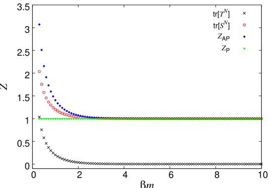
Figure 1: Partition function against $\beta m$ for $am=0.01$, $\lambda=1$, $K=150$ in $\phi^{6}$ theory. $Z_{\mathrm{P}}$ (green triangle) and $Z_{\mathrm{AP}}$ (blue square) are ones with periodic and anti-periodic boundary conditions, respectively. The traces of $T^{N}$ (black cross) and $S^{N}$ (red circle) are also presented.

The Gauss-Hermite quadrature with the scaling is employed in the computation. We have to choose the number of Gauss-Hermite points $K$ and the scale parameter $s$ for each $ma$. Although the approximation is expected to be improved as $K$ increases, we find that $K\simeq 150-200$ is large enough to show the convergence of results, for instance, as seen in Figure 2. For fixed $K$, we optimize $s$ such that the relative error $\delta=|Z_{P}-1|$ is smaller than $O(10^{-9})$. Figure 3 is an example of calculation for determining $s$. In this case, we have $\delta\lesssim{\cal O}(10^{-9})$ for $0.21\lesssim s\lesssim 0.24$.

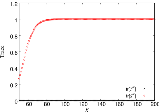
Figure 2: Traces of $T^{N}$ (black cross) and $S^{N}$ (red circle) with varying $K$, which are estimated for $N=3000$, $am=0.01$, $\lambda=1$ in $\phi^{6}$-theory.

Figure 3: $s$-dependence of $|Z_{\mathrm{P}}-1|$ for $N=30000$, $am=0.001$, $\lambda=1$, $K=200$.

Table 1 shows the parameters used to compute the energy eigenvalues and correlators of $\phi^{6}$ theory, chosen by the procedures above. We concentrate on the case of

$$\lambda=1,\qquad\beta m=30.$$ (46)

This value of $\lambda$ has been used in the previous Monte-Carlo studies. The continuum limit is achieved by taking $ma\rightarrow 0$ for fixed $\beta m$. In the table, we basically choose $N$ such that the lattice spacings are given in equal intervals as $ma=(\beta m)/N$. Same as the free theory, the scale parameter $s$ approaches zero as $ma$ decreases. Although we could not find $s$ that realizes $Z_{P}=1$ within errors of ${\cal O}(10^{-9})$ for $ma<0.001$ within $K\leq 200$, the lattice spacings are smaller than those used in the Monte-Carlo studies.

$am$	s	$N$	$K$
0.020	0.88	1500	150
0.019	0.86	1580
0.018	0.84	1670
0.017	0.82	1760
0.016	0.80	1880
0.015	0.78	2000
0.014	0.76	2140
0.013	0.74	2310	$\cdot$
0.012	0.72	2500	$\cdot$
0.011	0.70	2730	$\cdot$
0.010	0.68	3000
0.009	0.62	3330
0.008	0.60	3750
0.007	0.55	4290
0.006	0.5	5000
0.005	0.45	6000	150
0.004	0.44	7500	170
0.003	0.38	10000	170
0.002	0.32	15000	170
0.001	0.23	30000	200

Table 1: Parameters used in the computations of $\phi^{6}$ theory.

The energy eigenvalues can be read directly from the transfer matrices $S$ and $T$. As already mentioned in section 2.2, $S$ and $T$ correspond to two Hamiltonians in SUSY QM, $H_{B}$ and $H_{F}$. We can read the eigenvalues of bosonic states from $S={\rm exp}(-aH_{B})$ and ones of fermionic states from $T={\rm exp}(-aH_{F})$, and obtain $E^{B}_{i}$ and $E^{F}_{i}$ by diagonalizing the transfer matrices $S$ and $T$. We find that the lattice results satisfy (23) within the relative errors of ${\cal O}(10^{-9})$ in all parameters (finite lattice spacings), at least, for five smallest eigenvalues. This is because the one supersymmetry remains exactly on the lattice.

Figure 4 shows the five smallest non-zero energy eigenvalues for several lattice spacings. To extrapolate the values to the continuum limit, we use a fit formula,

$$E/m=a_{0}+a_{1}(ma)+a_{2}(ma)^{2}.$$ (47)

Note that $a_{0}$ is the value of $E/m$ at continuum limit. Table 2 shows the fit results. The main results are obtained from a fit for ten data points at small lattice spacings, while the errors are given by the largest difference between the main fit and other fits; one for twenty points, and fits using cubic polynomial for ten and twenty points. As explained above, $E_{i}\equiv E_{i}^{B}=E^{F}_{i}$ and $E^{B}_{0}=0$ within the relative errors of $O(10^{-9})$ for all lattice spacings. So the values given in this table are common for $E_{i}^{B}$ and $E^{F}_{i}$ because the errors of the extrapolation are larger than $O(10^{-9})$. The extrapolated values of $E/m$ can be determined in very high precision, within the errors less than $0.001$%.

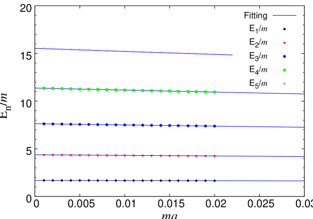
Figure 4: Energy spectra against the lattice spacing for $\phi^{6}$-theory. The lowest five eigenvalues are estimated for each $ma$ at fixed $\lambda=1$, $\beta m=30$.

	$E_{1}/m$	$E_{2}/m$	$E_{3}/m$	$E_{4}/m$	$E_{5}/m$
$a_{0}$	1.686497(3)	4.37180(2)	7.63091(4)	11.3748(1)	15.5396(2)
$a_{1}$	-1.897(2)	-6.417(9)	-13.29(2)	-22.39(5)	-33.69(8)
$a_{2}$	3.0(2)	12(1)	29(3)	55(5)	91(9)

Table 2: Energy eigenvalues of $\phi^{6}$ theory. The lowest five eigenvalues are obtained by using a fit, $E/m=a_{0}+a_{1}(ma)+a_{2}(ma)^{2}$, with $a_{0}$ the values of $E/m$ at the continuum limit.

In Figure 5, the correlation functions $\langle\phi_{N}\phi_{t}\rangle$ and $\langle\psi_{t}\overline{\psi}_{N}\rangle$ are shown as the black points and the red ones, respectively, in the case of $am=0.01$. Those points look like two curves since they are estimated for all $t$ without statistical errors. The correlators clearly show the exponential damping, and the slope is expected to be $E_{1}/m$. One can obtain any correlators in the same manner as $\langle\phi_{N}\phi_{t}\rangle$ and $\langle\psi_{t}\overline{\psi}_{N}\rangle$, namely, as very clear signals since there are no statistical uncertainties in our method.

Figure 5: Boson and fermion correlators for $am=0.01$, $\lambda=1$ in $\phi^{6}$ theory. The results of boson and fermion look like curves, but actually they are black and red points plotted for all $t$.

Although the energy eigenvalues can be read from the transfer matrices and were already shown above, let us apply the standard techniques to extract the effective masses from the correlation functions for the purpose of making a comparison our approach and Monte-Carlo method.

Figure 6 shows the effective masses defined by

$$m_{\mathrm{boson}}(t)\equiv\bigg{|}\log{\frac{\langle\phi_{N}\phi_{t}\rangle}{\langle\phi_{N}\phi_{t+1}\rangle}}\bigg{|},$$ (48)

$$m_{\mathrm{fermi}}(t)\equiv\bigg{|}\log{\frac{\langle\psi_{t}\overline{\psi}_{N}\rangle}{\langle\psi_{t+1}\overline{\psi}_{N}\rangle}}\bigg{|},$$ (49)

which are estimated for $ma=0.01$ ($N=3000$). The signals are also very clear without any statistical errors in comparison with the Monte-Carlo results. They are not constants since the high energy modes contribute near $t=0$ and the finite size effects are seen around $t=N/2$. The degenerated plateaus are seen for $0\ll t\ll N/2$. Estimating the effective masses at $t\simeq N/5=600$, we have $m_{\mathrm{fermi}}/m=1.6678215773620(2)$ and $m_{\mathrm{boson}}/m=1.667821577(1)$. The errors are estimated by varying $t$ from $500$ to $700$. This degeneracy is realized in the accuracy of nine digits. In Figure 7, the finite size effect is shown by changing $\beta m$ with the other parameters fixed. The masses are estimated at $t=[N/5]$. We find that $\beta m=30$ is large enough to obtain $m_{\rm eff}$ having no finite size effects.

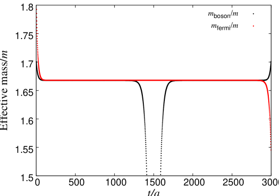
Figure 6: Effective masses $am_{\mathrm{boson}}(t)$ and $am_{\mathrm{fermi}}(t)$ for $N=3000$, $am=0.01$, $\lambda=1$.

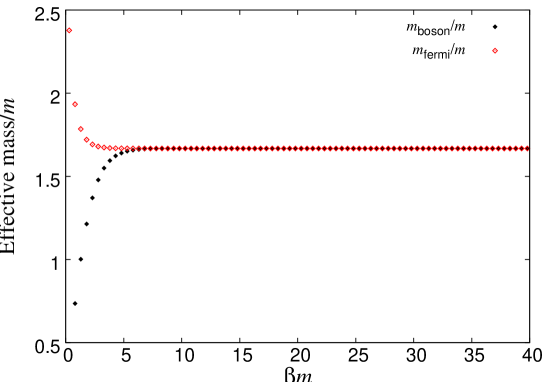
Figure 7: Finite volume effect of effective masses. We plot $am_{\mathrm{boson}}$ and $am_{\mathrm{fermi}}$ estimated at $t=[N/5]$ against $\beta m$, which are measured from the correlators for $am=0.01$, $\lambda=1$, $K=150$.

In Figure 8, an extrapolation to the continuum limit are shown for the effective masses estimated at $t=[N/5]$. We simply use the polynomials $f(x)=a_{0}+a_{1}x+a_{2}x^{2}$ as a fit function. The systematic errors of the fit are estimated in the same manner as the extrapolation of energy eigenvalues. The resultant effective mass is $m_{\mathrm{eff}}/m=1.686497(3)$ which is completely same as $E_{1}/m$ shown in Table 2.

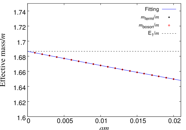
Figure 8: Continuum limit of effective masses. $am_{\mathrm{boson}}$ and $am_{\mathrm{fermi}}$, which are estimated at $t=N/5$ for $\lambda=1$, $\beta m=30$, are plotted.

Finally we show the numerical result of the SUSY Ward identity in the present lattice model. The SUSY Ward identity is used to show whether the broken supersymmetry is restored as a symmetry in the continuum limit. Consider the lattice supersymmetry transformation of $\langle\overline{\psi}_{N}\phi_{t}-\psi_{t}\phi_{N}\rangle$. Then one find that

$$\langle\delta(\overline{\psi}_{N}\phi_{t}-\psi_{t}\phi_{N})\rangle=\epsilon{\cal R}^{(1)}(t)+\overline{\epsilon}{\cal R}^{(2)}(t),$$ (50)

where

$${\cal R}^{(1)}(t)=-\langle\overline{\psi}_{N}\psi_{t}\rangle-\langle(\nabla_{-}\phi_{N}+W(\phi_{N}))\phi_{t}\rangle,$$ (51)

$${\cal R}^{(2)}(t)=-\langle\overline{\psi}_{N}\psi_{t}\rangle+\langle\phi_{N}(\nabla_{+}\phi_{t}+W(\phi_{t}))\rangle.$$ (52)

We can test whether full ${\cal N}=2$ supersymmetry are restored in the continuum limit by examining ${\cal R}^{(1)}(t)$ and ${\cal R}^{(2)}(t)$ because $\langle\delta(\overline{\psi}_{N}\phi_{t}-\psi_{t}\phi_{N})\rangle$ vanishes in the continuum theory.

Figure 12 shows numerical results of SUSY Ward identity for free theory ($\lambda=0$) and interacting case ($\lambda=1$). In the free theory, we observe that ${\cal R}^{(1)}(t)={\cal R}^{(2)}(t)=0$ within the error of ${\cal O}(10^{-9})$ for all $t$ since full ${\cal N}=2$ supersymmetry remain on the lattice. For interacting case, although ${\cal R}^{(1)}(t)$ vanishes for all $t$, ${\cal R}^{(2)}(t)$ does not. We found that it vanishes for $1\ll t/a\ll N$, and SUSY breaking effect does not survive at a scale lower than the cut-off. Thus we find that full ${\cal N}=2$ supersymmetry are restored in the continuum limit even for interacting case.

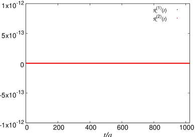
Figure 9: SUSY Ward identity in $\phi^{6}$ theory. Left figure shows the results in the free theory ($am=0.4$ and $\lambda=0$), and Right figure shows an interacting case ($am=0.01$ and $\lambda=1$).

4.2 Scarf I potential

The Scarf I model is characterized by the superpotential,

$$W(\phi)=\lambda\alpha\mathrm{tan}(\alpha\phi),$$ (53)

where $\alpha$ is a parameter with the mass dimension $1/2$ and $\lambda$ is the dimensionless coupling. This potential is one of SIPs, and the energy spectra are exactly solved as

$$\frac{E_{n}}{\alpha^{2}}=\frac{(2n\lambda+n^{2})}{2}.$$ (54)

We now take

$$\lambda=10,\qquad\beta\alpha^{2}=5,$$ (55)

to test our method in strong coupling region $\lambda\gg 1$. One find that the finite size effect is small enough by taking $\beta\alpha^{2}=5$, since it is of the order of $e^{-\beta E_{1}}$ and $\beta E_{1}\simeq 10\beta\alpha^{2}$.

Table 3 shows our parameters used in the computations of Scarf I model. We determine them using the same prescription as that of $\phi^{6}$ theory. We also use the Gauss-Legendre quadrature which is more effective than Gauss-Hermite method for small lattice spacings in the sense that $Z_{P}=1$ for smaller $K$ by choosing the scale parameter $s$.

$\alpha^{2}a$	s	$N$	$K$	Quadrature
0.00110	0.35	4550	150	Gauss-Hermite
0.00105	0.33	4760
0.00100	0.33	5000
0.00095	0.30	5260
0.00090	0.30	5560
0.00085	0.30	5880
0.00080	0.30	6250	$\cdot$
0.00075	0.29	6670	$\cdot$
0.00070	0.29	7140	$\cdot$
0.00065	0.28	7690
0.00060	0.275	8330
0.00055	0.275	9100
0.00050	0.27	10000
0.00045	0.27	11100	150
0.00040	0.013	12500	320	Gauss-Legendre
0.00035	0.012	14300	340
0.00030	0.012	16700	340
0.00025	0.011	20000	420
0.00020	0.010	25000	440
0.00015	0.008	33300	520
0.00010	0.007	50000	600

Table 3: Parameters in Scarf I model.

In Figure 10, the energy spectra obtained by our method are shown. Same as $\phi^{6}$-theory, the eigenvalues of $T$ and $S$ satisfy (23) within the errors of ${\cal O}(10^{-9})$. Table 4 shows the results of extrapolation to the continuum limit. We use a linear function to fit five data points at small lattice sizes, and the errors are estimated from the maximum of differences between the fit and ones for ten points and using quadratic polynomial. The obtained $a_{0}$ coincide with the exact solution within the small errors less than $0.001\%$.

Figure 10: Energy spectra against the lattice spacing for Scarf I model. The lowest five eigenvalues are estimated for each $\alpha^{2}a$ at fixed $\lambda=10$, $\beta\alpha^{2}=5$.

	$E_{1}/\alpha^{2}$	$E_{2}/\alpha^{2}$	$E_{3}/\alpha^{2}$	$E_{4}/\alpha^{2}$	$E_{5}/\alpha^{2}$
Exact	10.5	22	35	48	62.5
$a_{0}$	10.49998(2)	21.99996(5)	34.4999(1)	47.9999(2)	62.4998(2)
$a_{1}$	-57.7(1)	-131.9(3)	-224.0(5)	-335.5(8)	-468.0(12)

Table 4: Energy eigenvalues of Scarf I model. The lowest five eigenvalues are obtained by using a fit, $E/m=a_{0}+a_{1}(ma)$, with $a_{0}$ the values of $E/m$ at the continuum limit.

We also estimate the effective masses from correlators $\langle\phi_{N}\phi_{t}\rangle$ and $\langle\psi_{N}\overline{\psi}_{t}\rangle$ by the standard techniques used in the Monte-Carlo studies. The detailed procedures were already explained in $\phi^{6}$-theory. Figure 11 shows the extrapolation of effective masses to the continuum limit. We employ $f(x)=a_{0}+a_{1}x$ as a fit formula. The main fit and error estimation are performed in the same manner as energy eigenvalues in Table 4. Since the values at the continuum limit also reproduce the exact solutions with accuracy of $99.999\%$, we can say that the correlators are evaluated in high precision by our method.

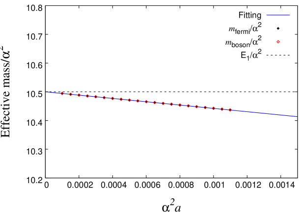
Figure 11: Continuum limit of effective masses. $am_{\mathrm{boson}}$ and $am_{\mathrm{fermi}}$ are estimated at $t=[N/5]$ for $\lambda=10$, $\beta\alpha^{2}=5$.

SUSY Ward identity is shown in Figure 12. ${\cal R}^{(1)}(t)$ vanishes for all $t$ thanks to the exact supersymmetry, while ${\cal R}^{(2)}(t)$ vanishes for $1\ll t\ll N$ as with the case of $\phi^{6}$-theory. Since two identities hold at a scale lower than the cut-off, full supersymmetry is restored in the continuum limit. In this way, one can confirm the supersymmetry restoration with high precision, compared to the Monte-Carlo method.

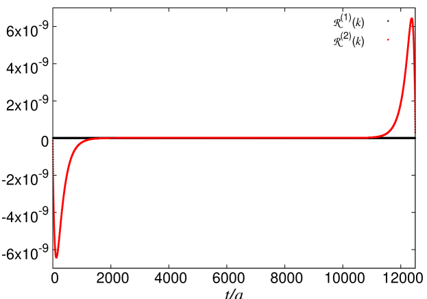
Figure 12: SUSY Ward identity in Scarf I model, which are estimated for $\lambda=10$ and $\beta\alpha^{2}=5$.

5 Conclusion and discussion

We have proposed a computational method based on the transfer matrix representation of lattice quantum mechanics. The numerical quadrature has been used to define the transfer matrices as finite dimensional ones, and Gaussian quadrature with rescaling variable went well even for interacting cases. We have tested our method for cubic and Scarf I potentials, and found that the energy eigenvalues and correlators can be evaluated in high precision within reasonable number of discretized points $K$.

Compared to Monte-Carlo method, stochastic processes are not needed to estimate the expectation values, and the sign problem does not exist in this method. The systematic error from finite-$K$ effect is well-controlled by taking larger $K$ and tuning the scale parameter $s$. The computational cost grows up with the logarithm of lattice size. Thus one can perform the computations at very small lattice spacings by taking large lattice sizes. Our method is useful for improving lattice SUSY models since one can examine the SUSY Ward identity and determine the cut-off dependence of physical quantities precisely.

Although we demonstrate our method in a specific lattice model of SUSY QM, the main idea of this paper is not limited to that case. Also, for non-SUSY models, a finite dimensional transfer matrix is defined by the numerical quadrature, and one can improve the method by rescaling variables. The scale parameter $s$ is chosen such that the Witten index reproduces the correct value for the present lattice SUSY model. However, a method of tuning $s$ is unknown for general models and remains an open question.

The higher dimensional theories could be studied by extending our method since the transfer matrix approach is related with not only TNR but also worldlines and worldsheets representation of $SU(N)$ gauge theory with fermions deForcrand:2009dh ; Marchis:2017oqi ; Gattringer:2017hhn . These kinds of extensions are applicable to higher dimensional models, and the techniques established in this paper could be useful.

- (1) E. Witten, Dynamical Breaking of Supersymmetry, Nucl. Phys. B188 (1981) 513.
- (2) E. Witten, Constraints on Supersymmetry Breaking, Nucl. Phys. B202 (1982) 253.
- (3) F. Cooper, A. Khare and U. Sukhatme, Supersymmetry and quantum mechanics, Phys. Rept. 251 (1995) 267–385, [hep-th/9405029].
- (4) L. E. Gendenshtein, Derivation of Exact Spectra of the Schrodinger Equation by Means of Supersymmetry, JETP Lett. 38 (1983) 356–359.
- (5) P. H. Dondi and H. Nicolai, Lattice Supersymmetry, Nuovo Cim. A41 (1977) 1.
- (6) S. Elitzur, E. Rabinovici and A. Schwimmer, Supersymmetric Models on the Lattice, Phys. Lett. 119B (1982) 165.
- (7) S. Elitzur and A. Schwimmer, Two-dimensional Wess-Zumino Model on the Lattice, Nucl. Phys. B226 (1983) 109–120.
- (8) S. Cecotti and L. Girardello, Stochastic Processes in Lattice (Extended) Supersymmetry, Nucl. Phys. B226 (1983) 417–428.
- (9) N. Sakai and M. Sakamoto, Lattice Supersymmetry and the Nicolai Mapping, Nucl. Phys. B229 (1983) 173–188.
- (10) M. F. L. Golterman and D. N. Petcher, A Local Interactive Lattice Model With Supersymmetry, Nucl. Phys. B319 (1989) 307–341.
- (11) Y. Kikukawa and Y. Nakayama, Nicolai mapping versus exact chiral symmetry on the lattice, Phys. Rev. D66 (2002) 094508, [hep-lat/0207013].
- (12) J. Giedt and E. Poppitz, Lattice supersymmetry, superfields and renormalization, J. High Energy Phys. 09 (2004) 029, [hep-th/0407135].
- (13) A. Feo, Predictions and recent results in SUSY on the lattice, Mod. Phys. Lett. A19 (2004) 2387–2402, [hep-lat/0410012].
- (14) M. Kato, M. Sakamoto and H. So, Taming the Leibniz Rule on the Lattice, JHEP 05 (2008) 057, [0803.3121].
- (15) D. Kadoh and H. Suzuki, Supersymmetric nonperturbative formulation of the WZ model in lower dimensions, Phys. Lett. B684 (2010) 167–172, [0909.3686].
- (16) D. Kadoh and H. Suzuki, Supersymmetry restoration in lattice formulations of 2D WZ model based on the Nicolai map, Phys. Lett. B696 (2011) 163–166, [1011.0788].
- (17) M. Kato, M. Sakamoto and H. So, A criterion for lattice supersymmetry: cyclic Leibniz rule, JHEP 05 (2013) 089, [1303.4472].
- (18) D. Kadoh and N. Ukita, General solution of the cyclic Leibniz rule, PTEP 2015 (2015) 103B04, [1503.06922].
- (19) K. Asaka, A. D’Adda, N. Kawamoto and Y. Kondo, Exact lattice supersymmetry at the quantum level for Wess-Zumino models in 1- and 2-dimensions, Int. J. Mod. Phys. A31 (2016) 1650125, [1607.04371].
- (20) M. Kato, M. Sakamoto and H. So, Non-renormalization theorem in a lattice supersymmetric theory and the cyclic Leibniz rule, PTEP 2017 (2017) 043B09, [1609.08793].
- (21) A. D’Adda, N. Kawamoto and J. Saito, An Alternative Lattice Field Theory Formulation Inspired by Lattice Supersymmetry, J. High Energy Phys. 12 (2017) 089, [1706.02615].
- (22) M. Beccaria, G. Curci and E. D’Ambrosio, Simulation of supersymmetric models with a local Nicolai map, Phys. Rev. D58 (1998) 065009, [hep-lat/9804010].
- (23) S. Catterall and E. Gregory, A Lattice path integral for supersymmetric quantum mechanics, Phys. Lett. B487 (2000) 349–356, [hep-lat/0006013].
- (24) S. Catterall and S. Karamov, Exact lattice supersymmetry: The Two-dimensional N=2 Wess-Zumino model, Phys. Rev. D65 (2002) 094501, [hep-lat/0108024].
- (25) J. Giedt, R. Koniuk, E. Poppitz and T. Yavin, Less naive about supersymmetric lattice quantum mechanics, JHEP 12 (2004) 033, [hep-lat/0410041].
- (26) J. Giedt, R-symmetry in the Q-exact (2,2) 2-D lattice Wess-Zumino model, Nucl. Phys. B726 (2005) 210–232, [hep-lat/0507016].
- (27) G. Bergner, T. Kaestner, S. Uhlmann and A. Wipf, Low-dimensional Supersymmetric Lattice Models, Annals Phys. 323 (2008) 946–988, [0705.2212].
- (28) I. Kanamori, F. Sugino and H. Suzuki, Observing dynamical supersymmetry breaking with euclidean lattice simulations, Prog. Theor. Phys. 119 (2008) 797–827, [0711.2132].
- (29) T. Kastner, G. Bergner, S. Uhlmann, A. Wipf and C. Wozar, Two-Dimensional Wess-Zumino Models at Intermediate Couplings, Phys. Rev. D78 (2008) 095001, [0807.1905].
- (30) G. Bergner, Complete supersymmetry on the lattice and a No-Go theorem, JHEP 01 (2010) 024, [0909.4791].
- (31) H. Kawai and Y. Kikukawa, A Lattice study of N=2 Landau-Ginzburg model using a Nicolai map, Phys. Rev. D83 (2011) 074502, [1005.4671].
- (32) I. Kanamori, A Method for Measuring the Witten Index Using Lattice Simulation, Nucl. Phys. B841 (2010) 426–447, [1006.2468].
- (33) C. Wozar and A. Wipf, Supersymmetry Breaking in Low Dimensional Models, Annals Phys. 327 (2012) 774–807, [1107.3324].
- (34) S. Schierenberg and F. Bruckmann, Improved lattice actions for supersymmetric quantum mechanics, Phys. Rev. D89 (2014) 014511, [1210.5404].
- (35) K. Steinhauer and U. Wenger, Spontaneous supersymmetry breaking in the 2D 1 Wess-Zumino model, Phys. Rev. Lett. 113 (2014) 231601, [1410.6665].
- (36) D. Baumgartner and U. Wenger, Supersymmetric quantum mechanics on the lattice: I. Loop formulation, Nucl. Phys. B894 (2015) 223–253, [1412.5393].
- (37) D. Baumgartner and U. Wenger, Supersymmetric quantum mechanics on the lattice: II. Exact results, Nucl. Phys. B897 (2015) 39–76, [1503.05232].
- (38) D. Baumgartner and U. Wenger, Supersymmetric quantum mechanics on the lattice: III. Simulations and algorithms, Nucl. Phys. B899 (2015) 375–394, [1505.07397].
- (39) M. Levin and C. P. Nave, Tensor renormalization group approach to 2D classical lattice models, Phys. Rev. Lett. 99 (2007) 120601, [cond-mat/0611687].
- (40) Y. Shimizu, Analysis of the -dimensional lattice model using the tensor renormalization group, Chin. J. Phys. 50 (2012) 749.
- (41) Y. Shimizu and Y. Kuramashi, Grassmann tensor renormalization group approach to one-flavor lattice Schwinger model, Phys. Rev. D90 (2014) 014508, [1403.0642].
- (42) Y. Shimizu and Y. Kuramashi, Critical behavior of the lattice Schwinger model with a topological term at using the Grassmann tensor renormalization group, Phys. Rev. D90 (2014) 074503, [1408.0897].
- (43) S. Takeda and Y. Yoshimura, Grassmann tensor renormalization group for the one-flavor lattice Gross-Neveu model with finite chemical potential, PTEP 2015 (2015) 043B01, [1412.7855].
- (44) H. Kawauchi and S. Takeda, Tensor renormalization group analysis of CP(N-1) model, Phys. Rev. D93 (2016) 114503, [1603.09455].
- (45) R. Sakai, S. Takeda and Y. Yoshimura, Higher order tensor renormalization group for relativistic fermion systems, PTEP 2017 (2017) 063B07, [1705.07764].
- (46) Y. Yoshimura, Y. Kuramashi, Y. Nakamura, S. Takeda and R. Sakai, Calculation of fermionic Green functions with Grassmann higher-order tensor renormalization group, 1711.08121.
- (47) Y. Shimizu and Y. Kuramashi, Berezinskii-Kosterlitz-Thouless transition in lattice Schwinger model with one flavor of Wilson fermion, Phys. Rev. D97 (2018) 034502, [1712.07808].
- (48) D. Kadoh, Y. Kuramashi, Y. Nakamura, R. Sakai, S. Takeda and Y. Yoshimura, Tensor network formulation for two-dimensional lattice Wess-Zumino model, 1801.04183.
- (49) P. de Forcrand and M. Fromm, Nuclear Physics from lattice QCD at strong coupling, Phys. Rev. Lett. 104 (2010) 112005, [0907.1915].
- (50) C. Marchis and C. Gattringer, Dual representation of lattice QCD with worldlines and worldsheets of abelian color fluxes, Phys. Rev. D97 (2018) 034508, [1712.07546].
- (51) C. Gattringer, D. Goschl and C. Marchis, Kramers-Wannier duality and worldline representation for the SU(2) principal chiral model, Phys. Lett. B778 (2018) 435–441, [1709.04691].