Communication-based Decentralized Cooperative Object Transportation Using Nonlinear Model Predictive Control
Abstract
This paper addresses the problem of cooperative transportation of an object rigidly grasped by robotic agents. We propose a Nonlinear Model Predictive Control (NMPC) scheme that guarantees the navigation of the object to a desired pose in a bounded workspace with obstacles, while complying with certain input saturations of the agents. The control scheme is based on inter-agent communication and is decentralized in the sense that each agent calculates its own control signal. Moreover, the proposed methodology ensures that the agents do not collide with each other or with the workspace obstacles as well as that they do not pass through singular configurations. The feasibility and convergence analysis of the NMPC are explicitly provided. Finally, simulation results illustrate the validity and efficiency of the proposed method.
Index Terms:
Multi-Agent Systems, Cooperative control, Decentralized Control, Manipulation, Object Transportation, Nonlinear Model Predictive Control, Collision Avoidance, Singularity Avoidance. Leader-follower ControlI Introduction
Over the last years, multi-agent systems have gained a significant amount of attention, due to the advantages they offer with respect to single-agent setups. Robotic manipulation is a field where the multi-agent formulation can play a critical role, since a single robot might not be able to perform manipulation tasks that involve heavy payloads and challenging maneuvers.
Regarding cooperative manipulation, the literature is rich with works that employ control architectures where the robotic agents communicate and share information with each other as well as completely decentralized schemes, where each agent uses only local information or observers [1, 2, 3, 4, 5, 6]. The most common methodology used in the related literature constitutes of impedance and force/motion control [1, 7, 8, 9, 10, 11, 12, 13, 14]. Most of the aforementioned works employ force/torque sensors to acquire knowledge of the manipulator-object contact forces/torques, which, however, may result to performance decline due to sensor noise.
Moreover, in manipulation tasks, such as pose/force or trajectory tracking, collision with obstacles of the environment has been dealt with only by exploiting the potential extra degrees of freedom of over-actuated agents, or by using potential field-based algorithms. These methodologies, however, may suffer from local minima, even in single-agent cases, and in many cases they yield high control inputs that do not comply with the saturation of actual motor inputs, especially close to collision configurations. In our previous works, [15, 16], we considered the problem of trajectory tracking for decentralized robust cooperative manipulation, without taking into account singularity- or collision avoidance.
Another important property that concerns robotic manipulators is the singularities of the Jacobian matrix, which maps the joint velocities of the agent to a D vector of generalized velocities. Such singular kinematic configurations, that indicate directions towards which the agent cannot move, must be always avoided, especially when dealing with task-space control in the end-effector [17]. In the same vein, representation singularities can also occur in the mapping from coordinate rates to angular velocities of a rigid body.
The main contribution of this work is to provide decentralized feedback control laws that guarantee the cooperative manipulation of an object in a bounded workspace with obstacles. In particular, given agents that rigidly grasp an object, we design decentralized control inputs for the navigation of the object to a final pose, while avoiding inter-agent collisions as well as collisions with obstacles. Moreover, we take into account constraints that emanate from control input saturation as well kinematic and representation singularities. The proposed approach to address this problem is the repeated solution of a Finite-Horizon Open-loop Optimal Control Problem (FHOCP) of each agent, by assigning a set of priorities. Control approaches using this strategy are referred to as Nonlinear Model Predictive Control (NMPC) (see e.g. [18, 19, 20, 21, 22, 23, 24, 25, 26, 27, 28, 29, 30]). A decentralized NMPC scheme has been considered in our submitted work [31], which concerns multi-agent navigation with inter-agent connectivity maintenance and collision avoidance.
In our previous work [28], a similar problem was considered in a centralized way. However, the computation burden is high, due to the fact that the number of states in the centralized case increases proportionally with the number of agents, causing exponential increase in the computational time and memory. In this work, we decouple the dynamic model among the object and the agents by using certain load-sharing coefficients and consider a communication-based leader agent formulation, where a leader agent determines the followed trajectory for the object and the follower agents comply with it through appropriate constraints. To the best of the authors’ knowledge, this is the first time that the problem of decentralized object transportation with singularity, obstacle and collision avoidance is addressed.
The remainder of the paper is structured as follows. Section II provides preliminary background. The system dynamics and the formal problem statement are given in Section III. Section IV discusses the technical details of the solution and Section V is devoted to a simulation example. Conclusions and future work are discussed in Section VI.
II Notation and Preliminaries
The set of positive integers is denoted as and the real -coordinate space, with , as ; and are the sets of real -vectors with all elements nonnegative and positive, respectively. The notation and , with , stands for positive semi-definite and positive definite matrices, respectively. The notation is used for the Euclidean norm of a vector and for the induced norm of a matrix . Given a real symmetric matrix , and denote the minimum and the maximum absolute value of eigenvalues of , respectively. Its minimum and maximum singular values are denoted by and respectively; and are the identity matrix and the matrix with all entries zeros, respectively. Given a set , we denote by its cardinality and by its -fold Cartesian product.
The vector connecting the origins of coordinate frames and } expressed in frame coordinates in -D space is denoted as . Given a vector is the skew-symmetric matrix defined according to . We further denote by the -- Euler angles representing the orientation of frame with respect to frame , where ; Moreover, is the rotation matrix associated with the same orientation and is the -D rotation group. The angular velocity of frame with respect to , expressed in frame coordinates, is denoted as and it holds that [17]. Define also the sets , . We define also the set
as the set of an ellipsoid in 3D, where is the center of the ellipsoid, the lengths of its three semi-axes and is an index term. The eigenvectors of matrix define the principal axes of the ellipsoid, and the eigenvalues of are: and . For notational brevity, when a coordinate frame corresponds to an inertial frame of reference , we will omit its explicit notation (e.g., ). Finally, all vector and matrix differentiations will be with respect to an inertial frame , unless otherwise stated.
Definition 1.
[32] A continuous function belongs to class if it is strictly increasing and . If and , then function belongs to class .
Lemma 1.
[33] Let be a continuous, positive-definite function, and be an absolutely continuous function in . Suppose that: , and . Then, it holds: .
III Problem Formulation
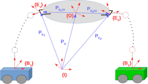
The formulation we adopt in this paper follows from the one from our previous work [28]. Consider a bounded and convex workspace , where is the workspace radius, consisting of robotic agents rigidly grasping an object, as shown in Fig. 1, and static obstacles described by the ellipsoids . The free space is denoted as . The agents are considered to be fully actuated and they consist of a base that is able to move around the workspace (e.g., mobile or aerial vehicle) and a robotic arm. The reference frames corresponding to the -th end-effector and the object’s center of mass are denoted with and , respectively, whereas corresponds to an inertial reference frame. The rigidity of the grasps implies that the agents can exert any forces/torques along every direction to the object. We consider that each agent knows the position and velocity only of its own state as well as its own and the object’s geometric parameters. Moreover, no interaction force/torque measurements or on-line communication is required.
III-A System model
III-A1 Robotic Agents
We denote by the joint space variables of agent , with , , where is the position and Euler-angle orientation of the agent’s base, and , are the degrees of freedom of the robotic arm. The overall joint space configuration vector is denoted as , with .
The linear and angular velocities of the agents’ base are described by the functions , with and , with , where is the representation Jacobian matrix, with:
We consider that each agent has access to its own state , and can compute, therefore the terms .
In addition, we denote as the position and Euler-angle orientation of agent ’s end-effector. More specifically, it holds that:
where are the forward kinematics of the robotic arm [17], and is the rotation matrix of the agent ’s base.
Let also denote a function that represents the generalized velocity of agent ’s end-effector, with being the angular velocity. Then, can be computed as:
| (1) |
where is the angular Jacobian of the robotic arm with respect to the agent’s base [17]. The differential kinematics (1) can be written as:
| (2) |
where the Jacobian matrix is given by:
Remark 1.
Note that becomes singular at representation singularities 111Other representations, such as rotation matrices or unit quaternions, do not exhibit such singularities. The prevent, however, global stabilization by continuous controllers due to topological obstructions., when and becomes singular at kinematic singularities defined by the set
In the following, we will aim at guaranteeing that will always be in the closed set:
for a small positive constant .
The joint-space dynamics for agent can be computed using the Lagrangian formulation:
| (3) |
where is the joint-space positive definite inertia matrix, represents the joint-space Coriolis matrix, is the joint-space gravity vector, is the generalized force vector that agent exerts on the object and is the vector of generalized joint-space inputs, with , where is the generalized force vector on the center of mass of the agent’s base and is the torque inputs of the robotic arms’ joints. By differentiating (2) we obtain:
| (4) |
By inverting (3) and using (2) and (4), we can obtain the task-space agent dynamics [17]:
| (5) |
with the corresponding task-space terms , , :
The task-space input wrench can be translated to the joint space inputs via
| (6) |
where belongs to the nullspace of and concerns over-actuated agents (see [17]). The term concerns over-actuated agents and does not contribute to end-effector forces.
We define by , the union of the ellipsoids that bound the -th agent’s volume, i.e., which is essentially the union of the ellipsoids that bound the volume of the agents’ links.
III-A2 Object Dynamics
Regarding the object, we denote its state as , , representing the pose and velocity of the object’s center of mass, with , , . The second order Newton-Euler dynamics of the object are given by:
| (7a) | ||||
| (7b) | ||||
where is the positive definite inertia matrix, is the Coriolis matrix, and is the gravity vector. In addition, is the object representation Jacobian , with
which is singular when . Finally, is the force vector acting on the object’s center of mass. Also, similarly to the robotic agents, we define by the bounding ellipsoid of the object.
III-A3 Coupled Dynamics
Consider robotic agents rigidly grasping an object. Then, the coupled system object-agents behaves like a closed-chain robot and we can express the object’s pose and velocity as a function of and , . Hence, In view of Fig. 1, we conclude that:
| (8a) | ||||
| (8b) | ||||
for every , where are local functions of the agents that provide the object’s pose, represents the constant distance and the relative orientation offset between the th agent’s end-effector and the object’s center of mass, which are considered known. The grasp rigidity implies that , . Therefore, by differentiating (8a), we can also express as a function of as
| (9) |
from which, we obtain:
| (10) |
where is a smooth mapping representing the Jacobian from the object to the -th agent:
| (11) |
and is always full rank due to the grasp rigidity.
Remark 2.
The Kineto-statics duality [17] along with the grasp rigidity suggest that the force acting on the object center of mass and the generalized forces , exerted by the agents at the contact points are related through:
| (12) |
where and is the grasp matrix, with and the matrix inverse of , .
Consider now the constants , with and , that play the role of load sharing coefficients for the agents. Then (7b) can be written as:
from which, by employing (12), (2), (4), (9) and (10), and after straightforward algebraic manipulations, we obtain the coupled dynamics:
| (13) |
where:
where and .
Remark 3.
Note that the agents dynamics under consideration hold for generic robotic agents comprising of a moving base and a robotic arm. Hence, the considered framework can be applied for mobile, aerial, or underwater manipulators.
Problem 1.
Consider robotic agents, rigidly grasping an object, governed by the coupled dynamics (13). Given a desired pose for the object, design the control inputs such that , while ensuring the satisfaction of the following collision avoidance and singularity properties:
-
1.
,
-
2.
,
-
3.
,
-
4.
,
-
5.
, ,
-
6.
, ,
, for , as well as the velocity and input constraints: , for some positive constants .
Regarding the joint velocity constraints, we impose for the arm joint velocities the constraint , which maximizes the manipulability ellipsoid of the arms [17], and hence increases robotic manipulability. Specifications in the aforementioned problem stand for collision avoidance between the agents, the objects, and the workspace obstacles and specifications stand for representation and kinematic singularities.
In order to solve the aforementioned problem, we need the following assumption regarding the workspace:
Assumption 1.
(Problem Feasibility Assumption) The set , is connected.
Assumption 2.
(Sensing and communication capabilities) Each agent is able to continuously measure the other agents’ state , . Moreover, each agent is able to communicate with the other agents without any delays.
Note that the aforementioned sensing assumption is reasonable, since in cooperative manipulation tasks, the agents are sufficiently close to each other, and therefore potential sensing radii formed by realistic sensors are large enough to cover them. Moreover, each agent can construct at every time instant the set-valued functions , , whose structure can be transmitted off-line to all agents. Let us define also the sets:
for every , associated with the desired collision-avoidance properties, where the notation stands for the stack vector of all , . Moreover, define the projection sets for agent as the set-valued functions:
where the notation stands for the stack vector of all .
IV Main Results
In this section, a systematic solution to Problem 1 is introduced. Our overall approach builds on designing a NMPC scheme for the system of the manipulators and the object. The proposed methodology is decentralized, since we do not consider a centralized system that calculates all the control signals and transmits them to the agents, like in our previous work [28]. As expected, this relaxes greatly the computational burden of the NMPC approach, which is also verified by the simulation results. To achieve that, we employ a leader-follower perspective. More specifically, as will be explained in the sequel, at each sampling time, a leader agent solves part of the coupled dynamics (13) via an NMPC scheme, and transmits its predicted variables to the rest of the agents. Assume, without loss of generality, that the leader corresponds to agent . Loosely speaking, the proposed solution proceeds as follows: agent solves, at each sampling time step, the receding horizon model predictive control subject to the forward dynamics:
| (14) |
and a number of inequality constraints, as will be clarified later. After obtaining a control input sequence and a set of predicted variables for , denoted as , it transmits the corresponding predicted state for the object for the control horizon to the other agents . Then, the followers solve the receding horizon NMPC subject to the forward dynamics:
| (15) |
and the state equality constraints:
| (16) |
as well as a number of inequality constraints that incorporate obstacle and inter-agent collision avoidance. More specifically, we consider that there is a priority sequence among the agents, which we assume, without loss of generality, that is defined by , and can be transmitted off-line to the agents. Each agent, after solving its optimization problem, transmits its calculated predicted variables to the agents of lower priority, which take them into account for collision avoidance. Note that the coupled object-agent dynamics are implicitly taken into account in equations (14), (15) in the following sense. Although the coupled model (13) does not imply that each one of these equations is satisfied, by forcing each agent to comply with the specific dynamics through the optimization procedure, we guarantee that (13) is satisfied, since it’s the result of the addition of (14) and (15), for every and , respectively. Intuitively, the leader agent is the one that determines the path that the object will navigate through, and the rest of the agents are the followers that contribute to the transportation. Moreover, the equality constraints (16) guarantee that the predicted variables of the agents will comply with the rigidity at the grasping points through the equality constraints (16).
By using the notation , , the nonlinear dynamics of each agent can be written as:
| (17) |
where is the locally Lipschitz function:
where , is the pseudo-inverse
and , . It can be proved that in the set the matrix has full rank and hence, is well defined for all . We define then the error vector , as:
which gives us the error dynamics:
| (18) |
where the function is given by:
Remark 4.
It can be concluded that is Lipschitz continuous in since it is continuously differentiable in its domain. Thus, for every , with , there exists a Lipschitz constant such that: .
From (6), we have that . Hence, the constraints for and , ,, can be written as coupled state-input constraints:
Let us now define the following sets :
| (19) |
as the sets that capture the control input constraints of (17), as well as their projections
| (20) |
Define also the set-valued functions , , by:
. Note that , .
The sets capture all the state constraints of the system dynamics (17), i.e., representation- and singularity-avoidance, collision avoidance among the agents and the obstacles, as well as collision avoidance of the object with the obstacles, which is assigned to the leader agent only We further define the set-valued functions by:
Note that only the leader agent is responsible for deriving a collision- and representation singularity-free path for the object.
The main problem at hand is the design of a feedback control law for agent which guarantees that the error signal with dynamics given in (18), satisfies , while ensuring singularity avoidance, collision avoidance between the agents, between the agents and the obstacles as well as the object and the obstacles. The role of the followers is, through the load-sharing coefficients in (13), to contribute to the object trajectory execution, as derived by the leader agent . In order to solve the aforementioned problem, we propose a NMPC scheme, that is presented hereafter.
Consider a sequence of sampling times , with a constant sampling period , , where is the prediction horizon, such that: , . Hereafter we will denote by the sampling instant. In sampled-data NMPC, a FHOCP is solved at the discrete sampling time instants based on the current state error information . The solution is an optimal control signal , computed over . For agent , the open-loop input signal applied in between the sampling instants is given by the solution of the following FHOCP:
| (21a) | |||
| subject to: | |||
| (21b) | |||
| (21c) | |||
| (21d) | |||
| (21e) | |||
At a generic time then, agent solves the aforementioned FHOCP. The notation is used to distinguish the predicted variables which are internal to the controller, corresponding to the system (21b). This means that is the solution of (21b) driven by the control input with initial condition . Note that, since the prediction horizon is finite, the predicted values are not the same with the actual closed-loop values (see [21]). In the following, we use the notation instead of for brevity. The functions , stand for the running cost and the terminal penalty cost, respectively, and they are defined as: , ; and are symmetric and positive definite controller gain matrices to be appropriately tuned; is a symmetric and positive semi-definite controller gain matrix to be appropriately tuned. The terminal set is chosen as:
where is an arbitrarily small constant to be appropriately tuned. The terminal set is used to enforce the stability of the closed-loop system.
The solution to FHOCP (21a) - (21e) at time provides an optimal control input, denoted by , . This control input is then applied to the system until the next sampling instant :
| (22) |
for every . At time a new FHOCP is solved in the same manner, leading to a receding horizon approach. The control input is of feedback form, since it is recalculated at each sampling instant based on the then-current state. The solution of (18) at time , , starting at time , from an initial condition , by application of the control input is denoted by:
The predicted state of the system (21b) at time , based on the measurement of the state at time , , by application of the control input as in (22), is denoted by , and the corresponding predicted error by:
After the solution of the FHOCP and the calculation of the predicted states
at each time instant , agent transmits the values , as well as and , as computed by (8), (9), to the rest of the agents . The rest of the agents then proceed as follows. Each agent , solves the following FHOCP:
| (23a) | |||
| subject to: | |||
| (23b) | |||
| (23c) | |||
| (23d) | |||
| (23e) | |||
| (23f) | |||
| (23g) | |||
at every sampling time . Note that, through the equality constraints (23e), (23f), the follower agents must comply with the trajectory computed by the leader . This can be problematic in the sense that this trajectory might drive the followers to collide with an obstacle or among each other, i.e., a solution to (23) might not exist. Resolution of such cases is not in the scope of this paper and constitutes part of future research. Here, we assume that there are no such cases:
Assumption 3.
The sets are nonempty, .
Next, similarly to the leader agent , it calculates the predicted states , which it transmits to the agents . In that way, at each time instant , each agent measures the other agents’ states (as stated in Assumption 2), incorporates the constraint (23c) for the agents , receives the predicted states from the agents and incorporates the collision avoidance constraint (23d) for the entire horizon. Loosely speaking, we consider that each agent takes into account the first state of the next agents in priority (), as well as the transmitted predicted variables of the previous agents in priority, for collision avoidance. Intuitively, the leader agent executes the planning for the followed trajectory of the object’s center of mass (through the solution of the FHOCP (21a)-(21e)), the follower agents contribute in executing this trajectory through the load sharing coefficients (as indicated in the coupled model (13)), and the agents low in priority are responsible for collision avoidance with the agents of higher priority. Moreover, the aforementioned equality constraints (23e), (23f) as well as the forward dynamics (23a) guarantee the compliance of all the followers with the model (13). For the followers, the cost can be selected as any function of , .
Therefore, given the constrained FHOCP (23a)-(23g), the solution of problem lies in the capability of the leader agent to produce a state trajectory that guarantess , by solving the FHOCP (21a)-(21e), which is discussed in Theorem 1.
Definition 2.
Theorem 1.
Proof.
The proof of the theorem consists of two parts: firstly, recursive feasibility is established, that is, initial feasibility is shown to imply subsequent feasibility; secondly, and based on the first part, it is shown that the error state reaches the terminal set . The feasibility analysis and the convergence analysis is similar with the proof of Theorem in [28, Section IV]. ∎
V Simulation Results
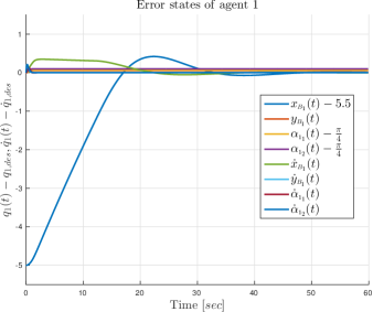
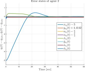
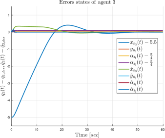
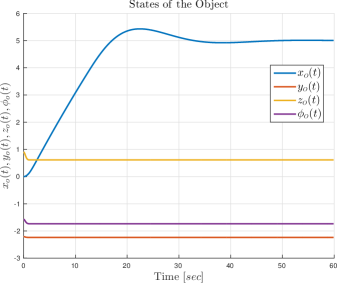
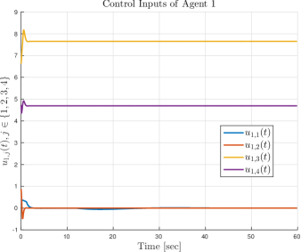
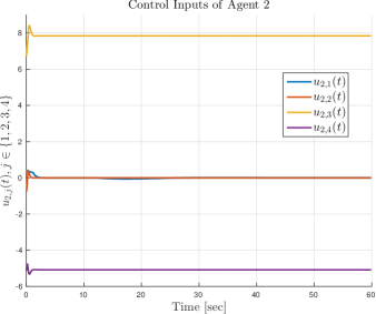
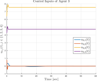
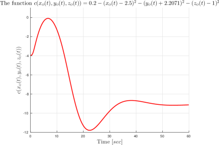
To demonstrate the efficiency of the proposed control protocol, we consider a simulation example with ground vehicles equipped with DOF manipulators, rigidly grasping an object with , . The states of the agents are given as: , , , , . The state of the object is and it is calculated though the states of the agents. The manipulators become singular when , thus the state constraints for the manipulators are set to: , , , . We also consider the input constraints: , , . The initial conditions of agents and the object are set to: , , , and . The desired goal state the object is set to , which, due to the structure of the considered robots, corresponding uniquely to , , , and . We set an obstacle between the initial and the desired pose of the object. The obstacle is spherical with center and radius . The sampling time is , the horizon is , and the total simulation time is ; The matrices , , are set to: , and the load sharing coefficients as , , and . The simulation results are depicted in Fig. 2- Fig. 9; Fig. 2, Fig. 3 and Fig. 4 show the error states of agent , and , respectively, which converge to ; Fig. 5 depicts the states of the objects; Fig. 9 shows the collision-avoidance constraint with the obstacle; Fig. 6 - Fig. 8 depict the control inputs of the three agents. Note that the different load-sharing coefficients produce slightly different inputs. The simulation was carried out by using the NMPC toolbox given in [24] and it took in MATLAB a Environment on a desktop with cores, GHz CPU and GB of RAM. In our previous work [28], the same simulation was centralized and it took on the same computer.
VI Conclusions and Future Work
In this work we proposed a NMPC scheme for decentralized cooperative transportation of an object rigidly grasped by robotic agents. The proposed control scheme deals with singularities of the agents, inter-agent collision avoidance as well as collision avoidance between the agents and the object with the workspace obstacles. We proved the feasibility and convergence analysis of the proposed methodology and simulation results verified the efficiency of the approach. Future efforts will be devoted towards reconfiguration in case of task infeasibility for the followers, event-triggered communication between the agents so as to reduce the communication burden that is required for solving the FHOCP at every sampling time, and real-time experiments.
References
- [1] S. Schneider and R. H. R. Cannon, “Object Impedance Control for Cooperative Manipulation: Theory and Experimental Results,” IEEE Transactions on Robotics and Automation, vol. 8, pp. 383–394, 1992.
- [2] Y.-H. Liu and S. Arimoto, “Decentralized Adaptive and Nonadaptive Position/Force Controllers for Redundant Manipulators in Cooperations,” The International Journal of Robotics Research, 1998.
- [3] M. Zribi and S. Ahmad, “Adaptive Control for Multiple Cooperative Robot Arms,” IEEE International Conference on Decision and Control (CDC), pp. 1392–1398, 1992.
- [4] O. Khatib, K. Yokoi, K. Chang, D. Ruspini, R. Holmberg, and A. Casal, “Decentralized Cooperation Between Multiple Manipulators,” IEEE International Workshop on Robot and Human Communication, pp. 183–188, 1996.
- [5] F. Caccavale, P. Chiacchio, and S. Chiaverini, “Task-Space Regulation of Cooperative Manipulators,” Automatica, 2000.
- [6] L. Gudiño-Lau, M. Arteaga, L. Munoz, and V. Parra-Vega, “On the Control of Cooperative Robots Without Velocity Measurements,” IEEE Transactions on Control Systems Technology, vol. 12, no. 4, pp. 600–608, 2004.
- [7] F. Caccavale, P. Chiacchio, A. Marino, and L. Villani, “Six-DOF Impedance Control of Dual-Arm Cooperative Manipulators,” IEEE/ASME Transactions On Mechatronics, vol. 13, no. 5, pp. 576–586, 2008.
- [8] D. Heck, D. Kostić, A. Denasi, and H. Nijmeijer, “Internal and External Force-Based Impedance Control for Cooperative Manipulation,” IEEE European Control Conference (ECC), pp. 2299–2304, 2013.
- [9] S. Erhart and S. Hirche, “Adaptive force/velocity control for multi-robot cooperative manipulation under uncertain kinematic parameters,” IEEE/RSJ International Conference on Intelligent Robots and Systems (IROS), pp. 307–314, 2013.
- [10] J. Szewczyk, F. Plumet, and P. Bidaud, “Planning and controlling cooperating robots through distributed impedance,” Journal of Robotic Systems, vol. 19, no. 6, pp. 283–297, 2002.
- [11] A. Tsiamis, C. K. Verginis, C. P. Bechlioulis, and K. J. Kyriakopoulos, “Cooperative Manipulation Exploiting only Implicit Communication,” IEEE/RSJ International Conference on Intelligent Robots and Systems (IROS), pp. 864–869, 2015.
- [12] F. Ficuciello, A. Romano, L. Villani, and B. B. Siciliano, “Cartesian Impedance Control of Redundant Manipulators for Human-Robot co-manipulation,” IEEE/RSJ International Conference on Intelligent Robots and Systems (IROS), pp. 2120–2125, 2014.
- [13] A. Ponce-Hinestroza, J. Castro-Castro, H. Guerrero-Reyes, V. Parra-Vega, and E. Olguỳn-Dỳaz, “Cooperative Redundant Omnidirectional Mobile Manipulators: Model-Fee Decentralized Integral Sliding Modes and Passive Velocity Fields,” IEEE International Conference on Robotics and Automation (ICRA), pp. 2375–2380, 2016.
- [14] W. Gueaieb, F. Karray, and S. Al-Sharhan, “A Robust Hybrid Intelligent Position/Force Control Scheme for Cooperative Manipulators,” IEEE/ASME Transactions on Mechatronics, pp. 109–125, 2007.
- [15] C. K. Verginis and D. V. Dimarogonas, “Distributed Cooperative Manipulation under Timed Temporal Specifications,” American Control Conference (ACC), 2017.
- [16] C. K. Verginis, M. Mastellaro, and D. V. Dimarogonas, “Robust Quaternion-based Cooperative Manipulation without Force/Torque Information,” IFAC World Congress, Toulouse, France, 2017.
- [17] B.Siciliano, L. Sciavicco, and L. Villani, “Robotics: Modelling, Planning and Control”. Advanced Textbooks in Control and Signal Processing, Springer, 2009.
- [18] D. Mayne, J. Rawlings, C. Rao, and P. Scokaert, “Constrained Model Predictive Control: Stability and Optimality,” Automatica, vol. 36, no. 6, pp. 789 – 814, 2000.
- [19] K. S. de Oliveira and M. Morari, “Contractive Model Predictive Control for Constrained Nonlinear Systems,” IEEE Transactions on Automatic Control, vol. 45, no. 6, pp. 1053–1071, 2000.
- [20] B. Kouvaritakis and M. Cannon, Nonlinear Predictive Control: Theory and Practice. No. 61, Iet, 2001.
- [21] R. Findeisen, L. Imsland, F. Allgower, and B. A. Foss, “State and Output Feedback Nonlinear Model Predictive Control: An Overview,” European Journal of Control, vol. 9, no. 2-3, pp. 190–206, 2003.
- [22] H. Chen and F. Allgöwer, “A Quasi-Infinite Horizon Nonlinear Model Predictive Control Scheme with Guaranteed Stability,” Automatica, vol. 34, no. 10, pp. 1205–1217, 1998.
- [23] R. Findeisen, L. Imsland, F. Allgöwer, and B. Foss, “Towards a Sampled-Data Theory for Nonlinear Model Predictive Control,” New Trends in Nonlinear Dynamics and Control and their Applications, pp. 295–311, 2003.
- [24] L. Grüne and J. Pannek, Nonlinear Model Predictive Control. Springer London, 2011.
- [25] E. Camacho and C. Bordons, “Nonlinear Model Predictive Control: An Introductory Review,” pp. 1–16, 2007.
- [26] J. Frasch, A. Gray, M. Zanon, H. Ferreau, S. Sager, F. Borrelli, and M. Diehl, “An Auto-Generated Nonlinear MPC Algorithm for Real-Time Obstacle Cvoidance of Ground Vehicles,” European Control Conference (ECC), 2013.
- [27] F. Fontes, “A General Framework to Design Stabilizing Nonlinear Model Predictive Controllers,” Systems and Control Letters, vol. 42, no. 2, pp. 127–143, 2001.
- [28] A. Nikou, C. K. Verginis, S. Heshmati-alamdari, and D. V. Dimarogonas, “A Nonlinear Model Predictive Control Scheme for Cooperative Manipulation with Singularity and Collision Avoidance,” 25th IEEE Mediterranean Conference on Control and Automation (MED), Valletta, Malta, 2017.
- [29] A. Nikou, S. Heshmati-alamdari, C. K. Verginis, and D. V. Dimarogonas, “Decentralized Abstractions and Timed Constrained Planning of a General Class of Coupled Multi-Agent Systems,” 56th IEEE Conference on Decision and Control (CDC), 2017.
- [30] A. Filotheou, A. Nikou, and D. V. Dimarogonas, “Decentralized Control of Uncertain Multi-Agent Systems with Connectivity Maintenance and Collision Avoidance,” IEEE European Control Conference (ECC), Limassol, Cyprus, 2017.
- [31] A. Filotheou, A. Nikou, and D. Dimarogonas, “Robust Decentralized Navigation of Multiple Rigid Bodies with Collision Avoidance and Connectivity Maintenance,” International Journal of Control (IJC), Under Review, 2017.
- [32] H. Khalil, Noninear Systems. Prentice-Hall, New Jersey, 1996.
- [33] H. Michalska and R. Vinter, “Nonlinear Stabilization Using Discontinuous Moving-Horizon Control,” IMA Journal of Mathematical Control and Information, vol. 11, no. 4, pp. 321–340, 1994.