Explicit Computational Wave Propagation in Micro-Heterogeneous Media

Abstract

Explicit time stepping schemes are popular for linear acoustic and elastic wave propagation due to their simple nature which does not require sophisticated solvers for the inversion of the stiffness matrices. However, explicit schemes are only stable if the time step size is bounded by the mesh size in space subject to the so-called CFL condition. In micro-heterogeneous media, this condition is typically prohibitively restrictive because spatial oscillations of the medium need to be resolved by the discretization in space. This paper presents a way to reduce the spatial complexity in such a setting and, hence, to enable a relaxation of the CFL condition. This is done using the Localized Orthogonal Decomposition method as a tool for numerical homogenization. A complete convergence analysis is presented with appropriate, weak regularity assumptions on the initial data.

Keywords explicit time stepping, hyperbolic equation, heterogeneous media, numerical homogenization, multiscale method

AMS subject classification 65M12, 65M60, 35L05

1 Introduction

We consider the discretization of the wave equation

$$\ddot{u}-\operatorname{div}A\nabla u =f \text{in }(0,T)\times\Omega,$$ (1.1)

$$u(0) =u_{0}\qquad \text{in }\Omega,$$

$$\dot{u}(0) =v_{0} \text{in }\Omega,$$

$$u|_{\Gamma} =0 \text{in }(0,T),$$

$$\nabla u\cdot\nu|_{\partial\Omega\setminus\Gamma} =0 \text{in }(0,T)$$

on a polygonal, convex, bounded Lipschitz domain $\Omega\subseteq\mathbb{R}^{d}$, $d\in\{2,3\}$ with outer normal $\nu$ and Dirichlet boundary $\Gamma\subseteq\partial\Omega$ with non-zero measure. Further, we assume that the initial data $u_{0}\in H^{1}_{\Gamma}(\Omega)$, $v_{0}\in L^{2}(\Omega)$ and the time-independent rough coefficient $A\in L^{\infty}(\Omega;\mathbb{R}^{d\times d}_{\mathrm{sym}})$ fulfills the bounds $\alpha|\xi|^{2}\leq A(x)\xi\cdot\xi$ and $|A(x)\xi|\leq\beta|\xi|$ for all $\xi\in\mathbb{R}^{d}$ and almost all $x\in\Omega$ for some $0<\alpha\leq\beta<\infty$. We have in mind coefficients that vary on some small scale $0<\varepsilon\ll 1$ but we do not need restrictive assumptions such as periodicity or scale separation.

In order to compute a numerical approximation of problem (1.1), we first write the problem in variational form, i.e., we seek a weak solution $u\in L^{2}(0,T;H^{1}_{\Gamma}(\Omega))$ with $\dot{u}\in L^{2}(0,T;L^{2}(\Omega))$ and $\ddot{u}\in L^{2}(0,T;H^{-1}(\Omega))$ such that

$$\langle\ddot{u},v\rangle_{H^{-1}(\Omega)\times H^{1}(\Omega)}+a(u,v)=(f,v)_{L^{2}(\Omega)}$$ (1.2)

for all $v\in H^{1}_{\Gamma}(\Omega)$ with initial conditions $u(0)=u_{0}$ and $\dot{u}(0)=v_{0}$, where $a$ denotes the bilinear form $a(u,v)\coloneqq\int_{\Omega}A\nabla u\cdot\nabla v\,dx$. Note that for any $u_{0}\in L^{2}(\Omega)$, $v_{0}\in H^{1}_{\Gamma}(\Omega)$ and $f\in L^{2}(0,T;L^{2}(\Omega))$, there exists a unique weak solution $u$ of (1.2). A proof of this can, for example, be found in [15, Ch. 7.2]. Restricting the solution space $H^{1}_{\Gamma}(\Omega)$ in (1.2) to a finite element space $V_{h}$ based on a regular mesh $\mathcal{T}_{h}$ of $\Omega$ with mesh size $h$ and applying the leapfrog scheme with step size $\Delta t$ in time leads to the following discrete problem:

Find $\mathbf{u_{h}}=(u_{h}^{n})_{n=0,...N}$ with $u_{h}^{n}\in V_{h}$ such that for $n\geq 2$

$$\Delta t^{-2}(u_{h}^{n+1}-2u_{h}^{n}+u_{h}^{n-1},v_{h})_{L^{2}(\Omega)}+a(u_{h}^{n},v_{h})=(f(n\Delta t),v_{h})_{L^{2}(\Omega)}$$ (1.3)

for all $v_{h}\in V_{h}$ and given $u_{h}^{0}$ and $u_{h}^{1}$.

It is well understood that such a method only leads to acceptable results if the mesh size $h$ is small enough to resolve the fine scale features in space originating from the highly varying coefficient $A$. Consider, for example, a coefficient that oscillates periodically between $\alpha$ and $\beta$ with period length $0<\varepsilon\ll 1$. In this case, the error of the finite element method scales at best like $(h/\varepsilon)^{s}$ for some $s>0$ that depends on the smoothness of $A$ and the domain $\Omega$. In order to obtain accuracy, at least $h<\varepsilon$ should hold. Such an $h$, however, may be too small to allow for reasonably fast computations. It is especially very restrictive since reducing the size of $h$ directly leads to larger systems of linear equations that need to be solved in every time step. Furthermore, the fact that the above method (1.3) is explicit in time also introduces the so-called CFL condition that limits the size of the time step $\Delta t$ by the (minimal) mesh size $h_{\text{min}}$, i.e., $\Delta t\lesssim h_{\text{min}}$. It is, hence, too expensive to pose the discrete problem on meshes with small mesh sizes $h$ that resolve fine scale features. The next section introduces a way to cope with the fine scale characteristics on an arbitrarily chosen coarse scale $H$ which not only reduces the size of present linear systems but also allows larger time steps subject to a relaxed CFL condition $\Delta t\lesssim H$.

The approach is based on the so-called Localized Orthogonal Decomposition method (LOD) introduced in [22] (see also [27]) and uses ideas similar to the ones presented in [29] for the wave equation in homogeneous media posed on domains with re-entrant corners. The basic idea of the method is to define low-dimensional finite element spaces that include spatial fine scale features. The construction is based on the decomposition of the solution space $H^{1}_{\Gamma}(\Omega)$ into an infinite-dimensional fine scale space and its finite-dimensional $a$-orthogonal complement. The latter has improved approximation properties compared to classical finite elements and may thus be used as both trial and test space for the spatial discretization. It can also be shown that there exists a bijective transformation from the classical finite element space to this improved approximation space. Thus, a basis of the new space is constructed by modifying the classical finite element basis functions by adding the solutions of auxiliary elliptic problems (so-called corrector problems). The corrector problems may even be localized without severely effecting approximation properties, which gives the method its name. The approach has been successfully applied to time-harmonic wave propagation to eliminate the pollution effect [28, 16, 8]. For the wave equation with rough coefficients, the LOD has already been used in combination with an implicit time discretization (Crank-Nicolson) in [2]. Therein, the need for additional regularity assumptions on the initial data is discussed, which is also crucial for the explicit time discretization in our case. Another possibility to resolve fine scale features in space is the Heterogeneous Multiscale Method (HMM) [11, 10], which is for instance discussed in [1, 12] or in [13, 4] in the context of wave propagation over long time. However, the HMM requires scale separation and may thus not be accurate in the general setting of this work. Another method for the numerical homogenization of the wave equation can be found in [24]. There, the idea is to use a harmonic coordinate transformation in order to obtain higher regularity of the weak solution. The main drawbacks of this approach are the necessary assumptions (so-called Cordes-type condition) that are hard to verify, and the approximation of the coordinate transformation for which global fine scale problems need to be solved. Another approach by the same authors is presented in [26], where so-called rough polyharmonic splines based on more demanding biharmonic corrector problems are introduced. A more recent approach [25] is based on a decomposition into orthogonal spaces in the spirit of the LOD method and shows the possible generalization of the present approach to a multilevel setting.

In general, any of the methods mentioned above can be used for the spatial discretization. The advantage of the LOD method is that it preserves the finite element structure of the problem and it is thus very convenient for practical applications. The use of an explicit time stepping scheme on the other side is motivated by its simple nature that allows for faster computations in every time step and by the fact that the discrete energy is conserved (see (2.8)). Since solutions to the wave equation conserve energy in the continuous setting, such a property is very natural and desirable in the discrete setting as well.

The paper is structured as follows. In Section 2, we introduce an idealized method based on the LOD method for the spatial discretization and the leapfrog scheme in time. We show stability and error estimates under suitable regularity assumptions and discuss a simplification of the method. Section 3 is devoted to a complete analysis of the fully discrete practical method, where also the auxiliary corrector problems are discretized in order to allow for practical computations. In Section 4, numerical experiments are presented to illustrate the numerical performance of the method and we give a short conclusion in Section 5.

In the remaining part of this paper we use the notations $(\bullet,\bullet)\coloneqq(\bullet,\bullet)_{L^{2}(\Omega)}$ and $\|\bullet\|\coloneqq\|\bullet\|_{L^{2}(\Omega)}$ for the standard $L^{2}$ scalar product and the corresponding norm. We denote with $V\coloneqq H^{1}_{\Gamma}(\Omega)$ the space $H^{1}(\Omega)$ with zero traces on $\Gamma$ and write $a\lesssim b$ if $a\leq Cb$ with a generic constant $C$ that can depend on the exact solution $u$ and its higher order time derivatives at time zero as well as the right-hand side $f$, in order to shorten the notation. Further, $\lesssim_{T}$ indicates linear dependence of the constant $C$ on $T$.

2 The Idealized Method

As mentioned above, the aim of this section is to discretize problem (1.2) on a coarse mesh with mesh size $H$ that does not resolve fine scale characteristics of the coefficient. The discrete solution should still achieve reasonably good accuracy. The general idea of the LOD is to ‘correct’ coarse finite element functions in such a way that they incorporate fine scale features of the given problem. The following subsection focuses on the spatial discretization and some useful properties. In subsection 2.2, we then introduce an idealized method and discuss its properties in the remaining subsections of this section.

2.1 Numerical upscaling by LOD

We consider a quasi-uniform shape regular mesh $\mathcal{T}_{H}$ on $\Omega$ with mesh size $H>\varepsilon$. The corresponding standard $P_{1}$/$Q_{1}$ finite element space is denoted by $V_{H}$. The construction of the modified finite element space is based on a projective quasi-interpolation operator $I_{H}\colon V\to V_{H}$ with approximation and stability properties, i.e.,

$$\|H^{-1}(v-I_{H}v)\|+\|\nabla I_{H}v\|\leq C_{I_{H}}\|\nabla v\|$$ (2.1)

for all $v\in V$ and

$$\|I_{H}v\|\leq C_{I_{H}}\|v\|$$ (2.2)

for all $v\in V$. The constant $C_{I_{H}}$ only depends on the shape regularity of the elements in the mesh but not on $H$. Ideally, such an operator is also local in the sense that the support of the interpolation is only marginally larger than the support of the original function. This is, for instance, the case with the following possible choice which is used for our numerical experiments, see [23, 5, 14, 20].

We define $I_{H}:=E_{H}\circ\Pi_{H}$, where $\Pi_{H}$ is the piecewise $L^{2}$ projection onto $P_{1}(\mathcal{T}_{H})$/ $Q_{1}(\mathcal{T}_{H})$, the space of piecewise linear/bilinear and possibly discontinuous functions that vanish at the boundary. $E_{H}$ denotes the averaging operator that maps $P_{1}(\mathcal{T}_{H})$/ $Q_{1}(\mathcal{T}_{H})$ to $V_{H}$ by assigning to each free vertex the arithmetic mean of the corresponding function values of the neighboring elements. Rigorously, for any $v\in P_{1}(\mathcal{T}_{H})$/$v\in Q_{1}(\mathcal{T}_{H})$ and a free vertex $z$ of $\mathcal{T}_{H}$, we have

$$(E_{H}(v))(z)=\sum_{T\in\mathcal{T}_{H}\atop\text{with }z\in T}v|_{T}(z)\cdot\mathrm{card}^{-1}\{K\in\mathcal{T}_{H}:z\in K\}.$$

With such an interpolation operator $I_{H}$ we can define the so-called fine scale space $W$ as its kernel, i.e., $W\coloneqq\mathrm{Ker}I_{H}$. We can then define for $v\in V$ the corrector $\mathcal{C}v\in W$ by

$$a(\mathcal{C}v,w)=a(v,w)$$ (2.3)

for all $w\in W$. Note that for any $v\in V$, it holds that

$$\alpha\|\nabla\mathcal{C}v\|^{2}\leq a(\mathcal{C}v,\mathcal{C}v)=a(v,\mathcal{C}v)\leq\beta\|\nabla v\|\|\nabla\mathcal{C}v\|,$$

and thus

$$\|\nabla\mathcal{C}v\|\leq\frac{\beta}{\alpha}\|\nabla v\|.$$

Similarly, we also obtain the estimate

$$\|\nabla\mathcal{C}v\|\leq\alpha^{-1}C_{I_{H}}H\|\operatorname{div}A\nabla v\|$$

if $\operatorname{div}A\nabla v\in L^{2}(\Omega)$ using the approximation property (2.1). Define $\tilde{V}_{H}\coloneqq(1-\mathcal{C})V_{H}$ and observe that $V=\tilde{V}_{H}\oplus W$ and $a(\tilde{V}_{H},W)=0$ by construction. Further, observe that the inverse inequality holds.

Lemma 2.1 (Inverse inequality).

For any $\tilde{v}_{H}\in\tilde{V}_{H}$,

$$\|\nabla\tilde{v}_{H}\|\leq\tilde{C}_{\mathrm{inv}}H^{-1}\|\tilde{v}_{H}\|.$$ (2.4)

Proof.

Let $\tilde{v}_{H}\in\tilde{V}_{H}$. Since $\tilde{v}_{H}=(1-\mathcal{C})I_{H}\tilde{v}_{H}$, we get

$$\begin{aligned} \alpha\|\nabla\tilde{v}_{H}\|^{2}&\leq a(\tilde{v}_{H},\tilde{v}_{H})=a(\tilde{v}_{H},I_{H}\tilde{v}_{H})\leq\beta\|\nabla\tilde{v}_{H}\|\|\nabla I_{H}\tilde{v}_{H}\|\\ &\leq\beta\|\nabla\tilde{v}_{H}\|C_{\mathrm{inv}}C_{I_{H}}H^{-1}\|\tilde{v}_{H}\|\end{aligned}$$

using (2.2) and the standard inverse inequality

$$\|\nabla v_{H}\|\leq C_{\mathrm{inv}}H^{-1}\|v_{H}\|$$ (2.5)

for any $v_{H}\in V_{H}$. Hence, (2.4) follows with $\tilde{C}_{\mathrm{inv}}\coloneqq C_{\mathrm{inv}}C_{I_{H}}\beta/\alpha$. ∎

Besides, the new space $\tilde{V}_{H}$ also has the following approximation property, which is a generalization of [29, Lemma 2.1] to the case of non-constant coefficients.

Lemma 2.2.

For all $u\in V$ with $\operatorname{div}A\nabla u\in L^{2}(\Omega)$, it holds that

$$\inf_{\tilde{v}_{H}\in\tilde{V}_{H}}\|u-\tilde{v}_{H}\|_{H^{1}(\Omega)}\leq\alpha^{-1}C_{I_{H}}H\|\operatorname{div}A\nabla u\|$$ (2.6)

Proof.

Let $\tilde{u}_{H}\in\tilde{V}_{H}$ be the orthogonal projection with respect to the bilinear form $a$ of $u$ onto $\tilde{V}_{H}$, i.e.,

$$a(\tilde{u}_{H},\tilde{v}_{H})=a(u,\tilde{v}_{H})$$

for all $\tilde{v}_{H}\in\tilde{V}_{H}$. Therefore, the error $e_{H}=u-\tilde{u}_{H}\in W$ and, hence,

$$\alpha\|\nabla e_{H}\|^{2}\leq a(e_{H},e_{H})=a(u,e_{H})=(-\operatorname{div}A\nabla u,e_{H})\leq\|\operatorname{div}A\nabla u\|\|e_{H}\|.$$

Since $e_{H}\in W$, it holds that

$$\|e_{H}\|=\|(1-I_{H})e_{H}\|\leq C_{I_{H}}H\|\nabla e_{H}\|$$

using the approximation property (2.1). Combining both inequalities results in

$$\|\nabla(u-\tilde{u}_{H})\|\leq\alpha^{-1}C_{I_{H}}H\|\operatorname{div}A\nabla u\|$$

which concludes the proof. ∎

2.2 Discretization in time

Based on the adapted spatial discretization defined above and the standard leapfrog scheme in time as in (1.3), the proposed idealized method reads:

Find $\mathbf{\tilde{u}_{H}}=(\tilde{u}_{n})_{n=0,..,N}$ with $\tilde{u}_{n}\in\tilde{V}_{H}$, such that for $n\geq 2$

$$\Delta t^{-2}(\tilde{u}_{n+1}-2\tilde{u}_{n}+\tilde{u}_{n-1},\tilde{v}_{H})+a(\tilde{u}_{n},\tilde{v}_{H})=(f(n\Delta t),\tilde{v}_{H})$$ (2.7)

for all $\tilde{v}_{H}\in\tilde{V}_{H}$ and given $\tilde{u}_{0}=(1-\mathcal{C})I_{H}u_{0}$ and suitable $\tilde{u}_{1}\in\tilde{V}_{H}$.

We call (2.7) the idealized method because we implicitly assume that the corrector problems (2.3) can be computed exactly. In order to show stability and error estimates for this scheme, standard methods can be applied [9, 19]. First, we introduce the discrete energy

$$\mathcal{E}^{n+1/2}(\mathbf{\tilde{u}_{H}})\coloneqq\frac{1}{2}(\|\dot{\tilde{u}}_{n+1/2}\|^{2}+a(\tilde{u}_{n},\tilde{u}_{n+1})),$$

where $\dot{\tilde{u}}_{n+1/2}\coloneqq\frac{\tilde{u}_{n+1}-\tilde{u}_{n}}{\Delta t}$ denotes the discrete time derivative. Using (2.7) with the test function $\tilde{v}_{H}=\tilde{u}_{n+1}-\tilde{u}_{n-1}$, we derive energy conservation in the sense that

$$\Delta t\,(f(n\Delta t),\dot{\tilde{u}}_{n+1/2}+\dot{\tilde{u}}_{n-1/2})$$ (2.8)

$$= \Delta t^{-2}(\tilde{u}_{n+1}-2\tilde{u}_{n}+\tilde{u}_{n-1},\tilde{u}_{n+1}-\tilde{u}_{n-1})+a(\tilde{u}_{n},\tilde{u}_{n+1}-\tilde{u}_{n-1})$$

$$= 2\left(\mathcal{E}^{n+1/2}(\mathbf{\tilde{u}_{H}})-\mathcal{E}^{n-1/2}(\mathbf{\tilde{u}_{H}})\right).$$

Lemma 2.3 (Stability of the idealized method).

Assume that the CFL condition

$$1-\frac{1}{2}\beta C_{\mathrm{inv}}^{2}C_{I_{H}}^{2}H^{-2}\Delta t^{2}\geq\delta$$ (2.9)

holds for some $\delta>0$. Then the idealized method (2.7) is stable, i.e.,

$$\|\dot{\tilde{u}}_{n+1/2}\|+\|\nabla\tilde{u}_{n+1}\|\leq C_{s}\left(\Delta t\sum_{k=1}^{n}\|f(k\Delta t)\|+\|\dot{\tilde{u}}_{1/2}\|+\|\nabla\tilde{u}_{0}\|+\|\nabla\tilde{u}_{1}\|\right)$$ (2.10)

with a generic constant $C_{s}$.

Proof.

The proof mainly follows the ideas presented in [9, 19], generalized to the case of arbitrary coefficients. With the inverse inequality (2.5) and the boundedness of the bilinear form $a$, i.e.,

$$a(u,v)\leq\beta\|\nabla u\|\|\nabla v\|$$

for any $u,v\in V$, we have

$$\quad\,\,\mathcal{E}^{n+1/2}(\mathbf{\tilde{u}_{H}})$$

$$=\frac{1}{2}\left(\|\dot{\tilde{u}}_{n+1/2}\|^{2}+a(\tilde{u}_{n},\tilde{u}_{n+1})\right)$$

$$=\frac{1}{4}a(\tilde{u}_{n+1},\tilde{u}_{n+1})+\frac{1}{4}a(\tilde{u}_{n},\tilde{u}_{n})-\frac{1}{4}a(\tilde{u}_{n+1}-\tilde{u}_{n},\tilde{u}_{n+1}-\tilde{u}_{n})+\frac{1}{2}\|\dot{\tilde{u}}_{n+1/2}\|^{2}$$

$$\geq\frac{1}{4}a(\tilde{u}_{n+1},\tilde{u}_{n+1})+\frac{1}{4}a(\tilde{u}_{n},\tilde{u}_{n})+\frac{1}{2}(1-\frac{1}{2}\beta C_{\text{inv}}^{2}C_{I_{H}}^{2}H^{-2}\Delta t^{2})\|\dot{\tilde{u}}_{n+1/2}\|^{2}$$

Here, we have used the fact that, for any $v_{H}\in V_{H}$,

$$a((1-\mathcal{C})v_{H},(1-\mathcal{C})v_{H})=a(v_{H},v_{H})-a(\mathcal{C}v_{H},\mathcal{C}v_{H})\leq\beta\|\nabla v_{H}\|^{2}.$$

The CFL condition (2.9) ensures positivity of the discrete energy, i.e.,

$$\mathcal{E}^{n+1/2}(\mathbf{\tilde{u}_{H}})\geq\frac{1}{4}a(\tilde{u}_{n+1},\tilde{u}_{n+1})+\frac{1}{4}a(\tilde{u}_{n},\tilde{u}_{n})+\frac{\delta}{2}\|\dot{\tilde{u}}_{n+1/2}\|^{2}.$$ (2.11)

With (2.8), we get the estimate

$$\mathcal{E}^{n+1/2}(\mathbf{\tilde{u}_{H}})-\mathcal{E}^{n-1/2}(\mathbf{\tilde{u}_{H}}) =\frac{1}{2}\Delta t(f(n\Delta t),\dot{\tilde{u}}_{n+1/2}+\dot{\tilde{u}}_{n-1/2})$$

$$\leq\frac{1}{2}\Delta t\|f(n\Delta t)\|(\|\dot{\tilde{u}}_{n+1/2}\|+\|\dot{\tilde{u}}_{n-1/2}\|)$$

$$\leq\frac{1}{\sqrt{2\delta}}\Delta t\|f(n\Delta t)\|\left(\sqrt{\mathcal{E}^{n+1/2}(\mathbf{\tilde{u}_{H}})}+\sqrt{\mathcal{E}^{n-1/2}(\mathbf{\tilde{u}_{H}})}\right)$$

using inequality (2.11). From this, we get

$$\sqrt{\mathcal{E}^{n+1/2}(\mathbf{\tilde{u}_{H}})}\leq\sqrt{\mathcal{E}^{n-1/2}(\mathbf{\tilde{u}_{H}})}+\frac{1}{\sqrt{2\delta}}\Delta t\|f(n\Delta t)\|$$

and, hence, the stability estimate

$$\sqrt{\mathcal{E}^{n+1/2}(\mathbf{\tilde{u}_{H}})}\leq\sqrt{\mathcal{E}^{1/2}(\mathbf{\tilde{u}_{H}})}+\frac{1}{\sqrt{2\delta}}\Delta t\sum_{k=1}^{n}\|f(k\Delta t)\|.$$

This, in turn, implies

$$\|\dot{\tilde{u}}_{n+1/2}\|+\|\nabla\tilde{u}_{n+1}\|\leq C_{s}\left(\Delta t\sum_{k=1}^{n}\|f(k\Delta t)\|+\|\dot{\tilde{u}}_{1/2}\|+\|\nabla\tilde{u}_{0}\|+\|\nabla\tilde{u}_{1}\|\right)$$

with $C_{s}=\text{max}\left\{\sqrt{\frac{2}{\delta}},\frac{2}{\sqrt{\alpha}}\right\}\text{max}\left\{\sqrt{\frac{2}{\delta}},\sqrt{\beta}\right\}$. ∎

As in [29], we can use the estimate (2.10) to derive an estimate for the error $\tilde{u}_{n}-u(t_{n})$ in the next subsection. Note that the constant in (2.10) crucially depends on the contrast $\beta/\alpha$ and thus also the constant in the error bound depends on $\beta/\alpha$.

2.3 Error analysis

In order to derive an error estimate, let $z_{H}\in L^{2}(0,T;\tilde{V}_{H})$ denote the auxiliary semi-discrete solution, i.e., $\dot{z}_{H}\in L^{2}(0,T;\tilde{V}_{H})$, $\ddot{z}_{H}\in L^{2}(0,T;\tilde{V}_{H})$ and $z_{H}$ solves

$$\left(\ddot{z}_{H}(t),\tilde{v}_{H}\right)_{L^{2}(\Omega)}+a(z_{H}(t),\tilde{v}_{H})=(f(t),\tilde{v}_{H})$$ (2.12)

for all $\tilde{v}_{H}\in\tilde{V}_{H}$ and all $t\in[0,T]$, with initial conditions $z_{H}(0)=(1-\mathcal{C})I_{H}u_{0}$ and $\dot{z}_{H}(0)=(1-\mathcal{C})I_{H}v_{0}$.

Remark 2.4.

With the above regularity assumptions $u_{0}\in H^{1}_{\Gamma}(\Omega)$, $v_{0}\in L^{2}(\Omega)$ and $f\in L^{2}(0,T;L^{2}(\Omega))$, there exists a unique solution $z_{H}$ of (2.12). The energy norm of $z_{H}$ can be bounded by the norms of the initial data $u_{0}$, $v_{0}$ and the right-hand side $f$. This follows from standard ODE theory due to the fact that (2.12) may be rewritten as a linear system of ODEs.

For the time discretization, let $N=\lceil T/\Delta t\rceil$ be the number of time steps. Similar to the estimates in [29], the total error can be split into the discretization error $(E^{n})_{n=0,\dots,N}$ in time defined by $E^{n}=\tilde{u}_{n}-z_{H}(n\Delta t)$, and the spatial discretization error $z_{H}(n\Delta t)-u(n\Delta t)=z_{H}(n\Delta t)-\Pi_{\tilde{V}_{H}}u(n\Delta t)-\rho(n\Delta t)$ with the best-approximation error $\rho(t)=u(t)-\Pi_{\tilde{V}_{H}}u(t)$. Here, $\Pi_{\tilde{V}_{H}}u(t)$ denotes the orthogonal projection of $u(t)$ onto $\tilde{V}_{H}$ with respect to the bilinear form $a$. Using (2.10), we get the following result.

Theorem 2.5 (Error of the idealized method).

If $\ddot{u}\in L^{1}(0,T;L^{2}(\Omega))$ and $\ddot{z}_{H}\in C(0,T;L^{2}(\Omega))$, it holds with $t_{n}=n\Delta t$ that

$$\left\|\frac{(\tilde{u}_{n+1}-u(t_{n+1}))-(\tilde{u}_{n}-u(t_{n}))}{\Delta t}\right\|+\|\nabla(\tilde{u}_{n+1}-u(t_{n+1}))\|$$ (2.13)

$$\leq C_{s}\left(\|\dot{E}^{1/2}\|+\|\nabla E^{1}\|+\left\|\dot{z}_{H}(0)-\Pi_{\tilde{V}_{H}}\dot{u}(0)\right\|+\|\nabla(z_{H}(0)-\Pi_{\tilde{V}_{H}}u(0))\|\right.$$

$$\qquad\qquad\;\left.+\left\|\frac{\rho(t_{n})-\rho(t_{n-1})}{\Delta t}\right\|+\|\nabla\rho(t_{n})\|+\int_{0}^{t_{n}}\left\|\ddot{\rho}(s)\right\|\,ds\right.$$

$$\qquad\qquad\;\left.+\sum_{k=1}^{n}\Delta t\left\|\frac{z_{H}(t_{k+1})-2z_{H}(t_{k})+z_{H}(t_{k-1})}{(\Delta t)^{2}}-\ddot{z}_{H}(t_{k})\right\|\right),$$

with the constant $C_{s}$ from (2.10).

With (2.6) and under the assumption of some additional regularity and appropriate initial conditions, the right-hand side of (2.13) scales like $H+\Delta t^{2}$.

Corollary 2.6 (Error of the idealized method).

Assume that $u\in C^{3}(0,T;L^{2}(\Omega))$, $\ddot{u}\in C(0,T;H^{1}(\Omega))$, $z_{H}\in C^{4}(0,T;L^{2}(\Omega))$ and $f\in C^{1}(0,T;L^{2}(\Omega))$ and that the corresponding norms are independent of the roughness of $A$, i.e., they do not grow when reducing the fine scale $\varepsilon$ on which the coefficient varies. Let $\tilde{u}_{H}(t)$ be the piecewise linear function that interpolates $\mathbf{\tilde{u}_{H}}$ in time. Then

$$\|u-\tilde{u}_{H}\|_{L^{2}(0,T;H^{1}_{\Gamma}(\Omega))}\lesssim_{T}H+\Delta t^{2}.$$

Note that the standard assumptions on $u$, $z_{H}$ and $f$ are $u\in C^{4}(0,T;L^{2}(\Omega))$, $z_{H}\in C^{4}(0,T;L^{2}(\Omega))$ and $f\in C^{2}(0,T;L^{2}(\Omega))$. However, with (2.1) and the fact that $\rho(t)\in W$ the above assumptions are sufficient to bound the fifth to seventh term in (2.13) by $H$.

2.4 Regularity

We shall finally show that the regularity conditions of Corollary 2.6 can be met for relevant classes of problems with arbitrarily rough coefficients that are characterized by the right-hand side $f$ and the initial conditions.

Lemma 2.7 (Regularity).

Let $u$ be the solution of (1.2) and $z_{H}$ the semi-discrete solution of (2.12). Suppose that $f\in H^{3}(0,T;L^{2}(\Omega))$ and

• $v_{0}\in H^{1}_{\Gamma}(\Omega)$,

• $\ddot{u}(0):=f(0)+\operatorname{div}A\nabla u_{0}\in H^{1}_{\Gamma}(\Omega)$,

• $u^{(3)}(0):=\dot{f}(0)+\operatorname{div}A\nabla v_{0}\in H^{1}_{\Gamma}(\Omega)$,

• $u^{(4)}(0):=\ddot{f}(0)+\operatorname{div}A\nabla\ddot{u}(0)\in L^{2}(\Omega)$.

Further assume that the corresponding norms can be bounded independently of the fine scale $\varepsilon$ on which $A$ varies. Then $u$ and $z_{H}$ satisfy the assumptions of Corollary 2.6, i.e., $u\in C^{3}(0,T;L^{2}(\Omega))$, $\ddot{u}\in C(0,T;H^{1}(\Omega))$ and $z_{H}\in C^{4}(0,T;L^{2}(\Omega))$.

Proof.

Differentiating (1.1) with respect to time and using the assumptions (A1)-(A4) shows that the time derivatives of $u$ solve wave-type equations as well. From [15, Ch. 7.2] we get the necessary regularity $u\in H^{4}(0,T;L^{2}(\Omega))$, from which it follows that $u\in C^{3}(0,T;L^{2}(\Omega))$. It further holds that $u\in H^{3}(0,T;H^{1}(\Omega))$ and thus $\ddot{u}\in C(0,T;H^{1}(\Omega))$.

It remains to show that $z_{H}\in C^{4}(0,T;L^{2}(\Omega))$. As above, we can differentiate (2.12) with respect to time. Further, we use the fact that the initial conditions are defined by $z_{H}^{(i)}(0)=(1-\mathcal{C})I_{H}u^{(i)}(0)\in\tilde{V}_{H}$ for $i=0,\dots,3$. Since solutions to equations of the form (2.12) are in $C^{2}(0,T;\tilde{V}_{H})$ by standard ODE theory, it follows that $z_{H}\in C^{4}(0,T;\tilde{V}_{H})$ which concludes the proof. ∎

Remark 2.8.

The regularity assumptions (A1)-(A4) and $f\in H^{3}(0,T;L^{2}(\Omega))$ on the initial data and the right-hand side correspond to the conditions in [2] for the implicit setting and are referred to as ‘well-prepared and compatible of order $3$’.

2.5 A simplified method

The regularity properties of the solution $u$ due to the assumptions (A1)-(A4) and $f\in H^{3}(0,T;L^{2}(\Omega))$ allow for the following simplification of the method defined in (2.7). First, observe that (2.7) can be written as an equation for standard finite element functions $\mathbf{{u}_{H}}=({u}_{n})_{n=0,..,N}$ with $u_{n}\in V_{H}$ using the explicit characterization $\tilde{u}_{n}=(1-\mathcal{C})u_{n}$, i.e.,

$$\Delta t^{-2}\left((1-\mathcal{C})(u_{n+1}-2u_{n}+u_{n-1}),(1-\mathcal{C})v_{H}\right)+a\left((1-\mathcal{C})u_{n},(1-\mathcal{C})v_{H}\right)$$

$$= \left(f(n\Delta t),(1-\mathcal{C})v_{H}\right)$$

for all $v_{H}\in V_{H}$. A slightly modified method with reduced computational costs seeks $\mathbf{\bar{u}_{H}}=(\bar{u}_{n})_{n=0,..,N}$ with $\bar{u}_{n}\in V_{H}$ such that

$$\Delta t^{-2}\left(\bar{u}_{n+1}-2\bar{u}_{n}+\bar{u}_{n-1},v_{H}\right)+a\left((1-\mathcal{C})\bar{u}_{n},(1-\mathcal{C})v_{H}\right)=\left(f(n\Delta t),v_{H}\right)$$ (2.14)

for all $v_{H}\in V_{H}$. Note that the solution of (2.14) also fulfills stability properties similar to (2.10). Analogically to (2.13), we can thus also show that

$$\|u-(1-\mathcal{C})\bar{u}_{H}\|_{L^{2}(0,T;H^{1}_{\Gamma}(\Omega))}\lesssim_{T}H+\Delta t^{2}$$

under the assumption that the regularity properties of Lemma 2.7 hold. Hence, it is reasonable to use the simplified method in practice. See also Chapter 4.

Remark 2.9.

The simplification in (2.14) might raise the question whether mass lumping is also a possible modification. Numerical experiments show that mass lumping only works if the coefficient is essentially constant and can have a significant effect on the convergence rate otherwise. This is related to the fact that for general coefficients additional $H^{2}$ regularity in space cannot be expected.

3 The Practical Method

The method discussed in Section 2 is idealized in the sense that we have implicitly assumed that the corrector problems (2.3) can be solved exactly. In practice, those problems are discretized and localized as explained in Section 3.1 and 3.2.

3.1 Discretization of fine scales

As a first step, the problems (2.3) are discretized using classical finite elements. To quantify the error introduced by such a procedure, let $\mathbf{\tilde{u}_{H}}=(\tilde{u}_{n})_{n=0,..,N}$ with $\tilde{u}_{n}=(1-\mathcal{C})u_{n}\in\tilde{V}_{H}$ be the solution of problem (2.7). Further, define for any $v_{H}\in V_{H}$ the discretized correction $\mathcal{C}_{h}v_{H}$ as the finite element solution of (2.3) based on a discrete space $W_{h}\subset W$ on a mesh $\mathcal{T}_{h}$ with mesh size $h\leq\varepsilon$, i.e., the mesh size is chosen small enough to resolve variations of the coefficient $A$. Note that $W_{h}\subset V_{h}$, with $V_{h}$ being the standard $P_{1}$/$Q_{1}$ finite element space based on the mesh $\mathcal{T}_{h}$. Denote by $\mathbf{\tilde{u}_{H,h}}=(\tilde{u}_{h,n})_{n=0,..,N}$ with $\tilde{u}_{h,n}=(1-\mathcal{C}_{h})u_{h,n}$ the solution of (2.7) in the space $(1-\mathcal{C}_{h})V_{H}$. The following lemma quantifies the difference of these two solutions.

Lemma 3.1 (Fine scale discretization error).

Under the assumptions of Lemma 2.3 and Lemma 2.7, it holds that

$$\left\|\frac{\tilde{u}_{n}-\tilde{u}_{n-1}}{\Delta t}-\frac{\tilde{u}_{h,n}-\tilde{u}_{h,n-1}}{\Delta t}\right\|+\|\nabla(\tilde{u}_{n}-\tilde{u}_{h,n})\|\lesssim_{T}d_{\tilde{V}_{H}}[V_{h}]+H^{-1}(d_{\tilde{V}_{H}}[V_{h}])^{2},$$

with the approximation error $d_{\tilde{V}_{H}}[V_{h}]$ defined by

$$d_{\tilde{V}_{H}}[V_{h}]\coloneqq\sup_{v\in\tilde{V}_{H}}\frac{\inf_{v_{h}\in V_{h}}\|\nabla(v-v_{h})\|}{\|\nabla v\|}.$$

Proof.

Observe that the error $\tilde{e}_{n}=(1-\mathcal{C})(u_{n}-u_{h,n})$ solves

$$\Delta t^{-2}\left(\tilde{e}_{n+1}-2\tilde{e}_{n}+\tilde{e}_{n-1},(1-\mathcal{C})v_{H}\right)+a\left(\tilde{e}_{n},(1-\mathcal{C})v_{H}\right)$$

$$= (-f(n\Delta t),(\mathcal{C}-\mathcal{C}_{h})v_{H})+\Delta t^{-2}(\tilde{u}_{h,n+1}-2\tilde{u}_{h,n}+\tilde{u}_{h,n-1},(\mathcal{C}-\mathcal{C}_{h})v_{H})$$

$$+\Delta t^{-2}((\mathcal{C}-\mathcal{C}_{h})(u_{h,n+1}-2u_{h,n}+u_{h,n-1}),(1-\mathcal{C})v_{H})$$

$$+a((\mathcal{C}-\mathcal{C}_{h})u_{h,n},(\mathcal{C}-\mathcal{C}_{h})v_{H})\eqqcolon F^{n}((1-\mathcal{C})v_{H})$$

for all $v_{H}\in V_{H}$. If ${F^{n}|}_{\tilde{V}_{H}}\in L^{2}(\Omega)$, we can derive a bound on the error using similar arguments as in the derivation of (2.10). First, we need to estimate $\|\nabla(\mathcal{C}-\mathcal{C}_{h})v_{H}\|$. Using the fact that the corrector problems (2.3) can be interpreted as saddle point problems, we obtain from finite element saddle point theory [6, Ch. 2.2.2] that

$$\|\nabla(\mathcal{C}-\mathcal{C}_{h})v_{H}\| \leq(1+C_{I_{H}})(1+\beta/\alpha)\inf_{v_{h}\in V_{h}}\|\nabla(\mathcal{C}v_{H}-v_{h})\|$$ (3.1)

$$\leq C_{*}\sup_{v\in\tilde{V}_{H}}\frac{\inf_{v_{h}\in V_{h}}\|\nabla(v-v_{h})\|}{\|\nabla v\|}\|\nabla\tilde{v}_{H}\|$$

$$=C_{*}\,d_{\tilde{V}_{H}}[V_{h}]\,\|\nabla\tilde{v}_{H}\|$$

with $C_{*}=(1+C_{I_{H}})(1+\beta/\alpha)$ and $\tilde{v}_{H}=(1-\mathcal{C})v_{H}$ or $\tilde{v}_{H}=(1-\mathcal{C}_{h})v_{H}$. Using (2.1), we further get

$$\|(\mathcal{C}-\mathcal{C}_{h})v_{H}\|\leq C_{I_{H}}H\,C_{*}\,d_{\tilde{V}_{H}}[V_{h}]\,\|\nabla\tilde{v}_{H}\|.$$ (3.2)

With (3.1), (3.2) and the inverse inequality (2.4), we can derive the following bound,

$$\sup_{\tilde{v}_{H}\in\tilde{V}_{H}}\frac{|F^{n}(\tilde{v}_{H})|}{\|\tilde{v}_{H}\|} \leq\quad\Bigg{(}C_{I_{H}}C_{*}\tilde{C}_{\mathrm{inv}}\Big{(}\|f(n\Delta t)\|+2\left\|\frac{\tilde{u}_{h,n+1}-2\tilde{u}_{h,n}+\tilde{u}_{h,n-1}}{\Delta t^{2}}\right\|\Big{)}$$

$$\quad+\,\,\beta C_{*}^{2}\tilde{C}_{\mathrm{inv}}H^{-1}\|\nabla\tilde{u}_{h,n}\|\,d_{\tilde{V}_{H}}[V_{h}]\Bigg{)}d_{\tilde{V}_{H}}[V_{h}]$$

$$\lesssim\quad\,d_{\tilde{V}_{H}}[V_{h}]+H^{-1}(d_{\tilde{V}_{H}}[V_{h}])^{2}.$$

Thus, using the above equations and the fact that, for any $v_{H},y_{H}\in V_{H}$,

$$\|(1-\mathcal{C})v_{H}-(1-\mathcal{C}_{h})y_{H}\|_{\bullet}\leq\|(1-\mathcal{C})(v_{H}-y_{H})\|_{\bullet}+\|(\mathcal{C}-\mathcal{C}_{h})y_{H}\|_{\bullet},$$

it follows as in the derivation of (2.10) that

$$\left\|\frac{\tilde{u}_{n}-\tilde{u}_{n-1}}{\Delta t}-\frac{\tilde{u}_{h,n}-\tilde{u}_{h,n-1}}{\Delta t}\right\|+\|\nabla(\tilde{u}_{n}-\tilde{u}_{h,n})\|\lesssim_{T}d_{\tilde{V}_{H}}[V_{h}]+H^{-1}(d_{\tilde{V}_{H}}[V_{h}])^{2}.$$

∎

Note that we have used the fact that $\Delta t^{-2}(\tilde{u}_{h,n+1}-2\tilde{u}_{h,n}+\tilde{u}_{h,n-1})$ can be bounded in $L^{2}$ independently of $\Delta t$ and $H$. To see this, let $\dot{\tilde{u}}_{h,n+1/2}=\Delta t^{-1}(\tilde{u}_{h,n+1}-\tilde{u}_{h,n})$ be the discrete time derivative and observe that $(\dot{\tilde{u}}_{h,n+1/2})_{n=0,...,N-1}$ solves

$$\Delta t^{-2}\left(\dot{\tilde{u}}_{h,n+3/2}-2\dot{\tilde{u}}_{h,n+1/2}+\dot{\tilde{u}}_{h,n-1/2}),\tilde{v}_{H}\right)+a\left(\dot{\tilde{u}}_{h,n+1/2},\tilde{v}_{H}\right)$$

$$= \left(\Delta t^{-1}(f((n+1)\Delta t)-f(n\Delta t)),\tilde{v}_{H}\right)$$

for all $\tilde{v}_{H}\in(1-\mathcal{C}_{h})V_{H}$. Therefore, with equation (2.10) and the regularity assumptions of Lemma 2.7 we can bound the $L^{2}$ norm of $\Delta t^{-2}(\tilde{u}_{h,n+1}-2\tilde{u}_{h,n}+\tilde{u}_{h,n-1})$ in terms of the initial data and the right-hand side.

3.2 Localization of correctors

As a next step, we want to define the solution $\mathbf{\tilde{u}^{\ell}_{H,h}}$ of the fully practical method and quantify the error between the solutions $\mathbf{\tilde{u}_{H,h}}$ and $\mathbf{\tilde{u}^{\ell}_{H,h}}$. The practical method reads:

Find $\mathbf{\tilde{u}^{\ell}_{H,h}}=(\tilde{u}^{\ell}_{h,n})_{n=0,..,N}$ with $\tilde{u}^{\ell}_{h,n}=(1-\mathcal{C}^{\ell}_{h})u^{\ell}_{h,n}\in(1-\mathcal{C}^{\ell}_{h})V_{H}$, such that
for $n\geq 2$

$$\Delta t^{-2}(\tilde{u}^{\ell}_{h,n+1}-2\tilde{u}^{\ell}_{h,n}+\tilde{u}^{\ell}_{h,n-1},\tilde{v}_{H})+a(\tilde{u}^{\ell}_{h,n},\tilde{v}_{H})=(f(n\Delta t),\tilde{v}_{H})$$ (3.3)

for all $\tilde{v}_{H}\in(1-\mathcal{C}^{\ell}_{h})V_{H}$ and given $\tilde{u}^{\ell}_{h,0}=(1-\mathcal{C}^{\ell}_{h})I_{H}u_{0}$ and suitable $\tilde{u}^{\ell}_{h,1}\in$
$(1-\mathcal{C}^{\ell}_{h})V_{H}$.

Here, for any $v_{H}\in V_{H}$, $\mathcal{C}^{\ell}_{h}v_{H}$ denotes the discretized solution of (2.3) which is restricted to computations on local patches with $\ell$ layers. To be more precise, we first rewrite the operator $\mathcal{C}_{h}\colon V_{H}\to W_{h}$ as

$$\mathcal{C}_{h}v_{H}=\mathcal{C}_{h}\left(\sum_{T\in\mathcal{T}_{H}}v_{H}|_{T}\right)=\mathcal{C}_{h}\left(\sum_{T\in\mathcal{T}_{H}}\sum_{i=1}^{n_{T}}v_{H}(x_{T,i})\Lambda_{T,i}\right)=\sum_{T\in\mathcal{T}_{H}}\sum_{i=1}^{n_{T}}v_{H}(x_{T,i})q_{T,i},$$

where $x_{T,i},\ i=1,\dots n_{T}$ denote the corner points of $T$ and $\Lambda_{T,i}$ the corresponding nodal basis functions on $T$. Further, the element correctors $q_{T,i}\in W_{h}$ are defined by

$$a(q_{T,i},w_{h})=a|_{T}(\Lambda_{T,i},w_{h})$$

for all $w_{h}\in W_{h}$, where $a|_{T}(u,v)\coloneqq\int_{T}A\nabla u\cdot\nabla v\,dx$. Similarly, we can define the operator $\mathcal{C}^{\ell}_{h}\colon V_{H}\to W_{h}$ by

$$\mathcal{C}^{\ell}_{h}v_{H}=\sum_{T\in\mathcal{T}_{H}}\sum_{i=1}^{n_{T}}v_{H}(x_{T,i})q^{\ell}_{T,i},$$

where the localized element correctors $q^{\ell}_{T,i}\in W_{h}(\mathcal{N}^{\ell}(T))$ are given by

$$a(q^{\ell}_{T,i},w_{h})=a|_{T}(\Lambda_{T,i},w_{h})$$

for all $w_{h}\in W_{h}(\mathcal{N}^{\ell}(T))$. Here, $\mathcal{N}^{\ell}(T)$ is the extension of $T$ by $\ell$ layers of elements and $W_{h}(\mathcal{N}^{\ell}(T))$ the restriction of $W_{h}$ to functions with support in $\mathcal{N}^{\ell}(T)$. See also [22] for further details. Alternatively, the operator $\mathcal{C}^{\ell}_{h}$ could be defined as the $\ell$th iterate of some preconditioned solver based on an overlapping domain decomposition, as shown in [20].

The computation of the correctors is done during the offline stage and can be parallelized. Furthermore, periodic structure may be exploited. The additional cost to solve the corrector problems is moderate and the main advantage of the method lies in the online stage, where smaller linear systems need to be solved and relatively coarse time steps (subject to the CFL condition) may be used.

Lemma 3.2 (Localization error).

Suppose that the assumptions of Lemma 2.3 and Lemma 2.7 hold. Then

$$\left\|\frac{\tilde{u}_{h,n}-\tilde{u}_{h,n-1}}{\Delta t}-\frac{\tilde{u}^{\ell}_{h,n}-\tilde{u}^{\ell}_{h,n-1}}{\Delta t}\right\|+\|\nabla(\tilde{u}_{h,n}-\tilde{u}^{\ell}_{h,n})\|\lesssim_{T}\ell^{d/2}e^{-c\ell}+H^{-1}\ell^{d}e^{-2c\ell}.$$

Proof.

Similar to the findings in Lemma 3.1, the error $\tilde{e}_{n}^{\ell}=(1-\mathcal{C}_{h})(u_{h,n}-u^{\ell}_{h,n})$ solves

$$\Delta t^{-2}\left(\tilde{e}^{\ell}_{n+1}-2\tilde{e}^{\ell}_{n}+\tilde{e}^{\ell}_{n-1},(1-\mathcal{C}_{h})v_{H}\right)+a\left(\tilde{e}^{\ell}_{n},(1-\mathcal{C}_{h})v_{H}\right)$$

$$= (-f(n\Delta t),(\mathcal{C}_{h}-\mathcal{C}^{\ell}_{h})v_{H})+\Delta t^{-2}(\tilde{u}^{\ell}_{h,n+1}-2\tilde{u}^{\ell}_{h,n}+\tilde{u}^{\ell}_{h,n-1},(\mathcal{C}_{h}-\mathcal{C}^{\ell}_{h})v_{H})$$

$$+\Delta t^{-2}((\mathcal{C}_{h}-\mathcal{C}^{\ell}_{h})(u^{\ell}_{h,n+1}-2u^{\ell}_{h,n}+u^{\ell}_{h,n-1}),(1-\mathcal{C}_{h})v_{H})$$

$$+a((\mathcal{C}_{h}-\mathcal{C}^{\ell}_{h})u^{\ell}_{h,n},(\mathcal{C}_{h}-\mathcal{C}^{\ell}_{h})v_{H})\eqqcolon F_{h}^{n}((1-\mathcal{C}_{h})v_{H})$$

for all $v_{H}\in V_{H}$. As above, we want to show that ${F_{h}^{n}|}_{(1-\mathcal{C}_{h})V_{H}}\in L^{2}(\Omega)$. In [18, 22], it is shown that for any $v_{H}\in V_{H}$

$$\|\nabla(\mathcal{C}_{h}-\mathcal{C}^{\ell}_{h})v_{H}\|\leq C\ell^{d/2}e^{-c\ell}\|\nabla v_{H}\|$$

and thus also

$$\|(\mathcal{C}_{h}-\mathcal{C}^{\ell}_{h})v_{H}\|\leq C\ell^{d/2}e^{-c\ell}C_{I_{H}}H\|\nabla v_{H}\|,$$

see also [21, 20] for an alternative constructive proof. Similar to the estimates in Section 3.1, we obtain

$$\sup_{\tilde{v}_{H}\in(1-\mathcal{C}_{h})V_{H}}\frac{|F_{h}^{n}(\tilde{v}_{H})|}{\|\tilde{v}_{H}\|} \leq\quad\Bigg{(}CC^{2}_{I_{H}}C_{\mathrm{inv}}\Big{(}\|f(n\Delta t)\|+2\left\|\frac{\tilde{u}^{\ell}_{h,n+1}-2\tilde{u}^{\ell}_{h,n}+\tilde{u}^{\ell}_{h,n-1}}{\Delta t^{2}}\right\|\Big{)}$$

$$\quad+\,\,\beta C^{2}C_{I_{H}}C_{\mathrm{inv}}H^{-1}\|\nabla\tilde{u}^{\ell}_{h,n}\|\,\ell^{d/2}e^{-c\ell}\Bigg{)}\ell^{d/2}e^{-c\ell}$$

$$\lesssim\quad\,\ell^{d/2}e^{-c\ell}+H^{-1}\ell^{d}e^{-2c\ell}$$

and finally

$$\left\|\frac{\tilde{u}_{h,n}-\tilde{u}_{h,n-1}}{\Delta t}-\frac{\tilde{u}^{\ell}_{h,n}-\tilde{u}^{\ell}_{h,n-1}}{\Delta t}\right\|+\|\nabla(\tilde{u}_{h,n}-\tilde{u}^{\ell}_{h,n})\|\lesssim_{T}\ell^{d/2}e^{-c\ell}+H^{-1}\ell^{d}e^{-2c\ell}.$$

∎

3.3 Error of the practical method

We can now formulate the following theorem using Lemma 3.1, Lemma 3.2 and the triangle inequality.

Theorem 3.3 (Error of the practical method).

Let $u$ be the solution of (1.2) and assume that $\mathrm{(A1)}$-$\mathrm{(A4)}$ and $f\in H^{3}(0,T;L^{2}(\Omega))$ hold and $\Delta t\lesssim H$ subject to the CFL condition (2.9). Further, let $\mathbf{\tilde{u}^{\ell}_{H,h}}$ be the solution of the practical method and $\tilde{u}^{\ell}_{H,h}(t)$ the piecewise linear function that interpolates $\mathbf{\tilde{u}^{\ell}_{H,h}}$ in time. Then

$$\|u-\tilde{u}^{\ell}_{H,h}\|_{L^{2}(0,T;H^{1}_{\Gamma}(\Omega))}$$ (3.4)

$$\lesssim_{T} H+\Delta t^{2}+d_{\tilde{V}_{H}}[V_{h}]+H^{-1}(d_{\tilde{V}_{H}}[V_{h}])^{2}+\ell^{d/2}e^{-c\ell}+H^{-1}\ell^{d}e^{-2c\ell}.$$

If $\ell\gtrsim|\log H|$, (3.4) simplifies to

$$\|u-\tilde{u}^{\ell}_{H,h}\|_{L^{2}(0,T;H^{1}_{\Gamma}(\Omega))}\lesssim_{T}H+\Delta t^{2}+d_{\tilde{V}_{H}}[V_{h}]+H^{-1}(d_{\tilde{V}_{H}}[V_{h}])^{2}.$$

Theorem 3.3 shows that in order to obtain a reasonable error of order $H$, the error introduced by the discretization of the corrector problems (2.3) and thus the approximation error $d_{\tilde{V}_{H}}[V_{h}]$ need to be of order $H$ as well. The following lemma quantifies the approximation error $d_{\tilde{V}_{H}}[V_{h}]$ under additional regularity assumptions on the coefficient $A$.

Lemma 3.4.

Suppose that $A\in W^{1,\infty}(\Omega;\mathbb{R})$ with oscillations on the scale $\varepsilon$. Further, let $I_{h}\colon V\to V_{h}$ be a quasi-interpolation operator that fulfills properties similar to (2.1) and (2.2) with $h$ instead of $H$. Then,

$$d_{\tilde{V}_{H}}[V_{h}]\lesssim h(H^{-1}+\varepsilon^{-1}).$$

Proof.

For any $\tilde{v}_{H}\in\tilde{V}_{H}$, we have

$$\inf_{v_{h}\in V_{h}}\|\nabla(\tilde{v}_{H}-v_{h})\| \leq\|\nabla(1-I_{h})\tilde{v}_{H}\|\leq C_{I_{h}}h\|D^{2}\tilde{v}_{H}\|$$

$$\leq C_{I_{h}}h\|\Delta\tilde{v}_{H}\|\leq\frac{h}{\alpha}C_{I_{h}}\|A\Delta\tilde{v}_{H}\|$$

$$\leq\frac{h}{\alpha}C_{I_{h}}\left(\|\operatorname{div}A\nabla\tilde{v}_{H}\|+\|A\|_{W^{1,\infty}(\Omega;\mathbb{R})}\|\nabla\tilde{v}_{H}\|\right)$$

$$\leq\frac{h}{\alpha}C_{I_{h}}\left(\beta C_{\text{inv}}C_{I_{H}}H^{-1}+c\varepsilon^{-1}\right)\|\nabla\tilde{v}_{H}\|,$$

using the fact that $\|A\|_{W^{1,\infty}(\Omega;\mathbb{R})}\lesssim c\varepsilon^{-1}$ and

$$\|\operatorname{div}A\nabla\tilde{v}_{H}\|\leq\beta C_{\text{inv}}C_{I_{H}}H^{-1}\|\nabla\tilde{v}_{H}\|.$$ (3.5)

To show this, let $v\in C_{c}^{\infty}(\Omega)$ and observe that

$$\frac{|(\operatorname{div}A\nabla\tilde{v}_{H},v)|}{\|v\|} =\frac{|a(\tilde{v}_{H},v)|}{\|v\|}=\frac{|a(\tilde{v}_{H},I_{H}v)|}{\|v\|}\leq\frac{\beta\|\nabla\tilde{v}_{H}\|\|\nabla I_{H}v\|}{\|v\|}$$

$$\leq\beta C_{\mathrm{inv}}C_{I_{H}}H^{-1}\|\nabla\tilde{v}_{H}\|$$

employing the estimates (2.2) and (2.5). The inequality (3.5) then follows by the density of $C_{c}^{\infty}$ in $L^{2}$. Therefore, $d_{\tilde{V}_{H}}[V_{h}]$ can be bounded by

$$d_{\tilde{V}_{H}}[V_{h}]\lesssim h(H^{-1}+\varepsilon^{-1}).$$

∎

Using Theorem 3.3 and Lemma 3.4, we obtain the following result.

Corollary 3.5 (Error of the practical method).

Assume that $\mathrm{(A1)}$-$\mathrm{(A4)}$ and $f\in H^{3}(0,T;L^{2}(\Omega))$ hold. Assume further that $A\in W^{1,\infty}(\Omega;\mathbb{R})$, $\Delta t\lesssim H$ subject to the CFL condition (2.9), $\ell\gtrsim|\log H|$ and $h\lesssim H\varepsilon$. Then

$$\|u-\tilde{u}^{\ell}_{H,h}\|_{L^{2}(0,T;H^{1}_{\Gamma}(\Omega))}\lesssim_{T}H+\Delta t^{2}.$$

While orders of convergence in space and time appear imbalanced when the error is measured in $L^{2}(0,T;H^{1}_{\Gamma}(\Omega))$, quadratic convergence is empirically observed for the $L^{2}(0,T;L^{2}(\Omega))$ norm. In this sense, the error estimates of our explicit method are competitive with the fully implicit Crank-Nicolson approach of [2] provided that the fine scale discretization errors of [2] can be bounded by $(h/\varepsilon)^{2}$.

Remark 3.6.

The assumptions on the fine mesh size $h$ in Corollary 3.5 are in line with the theoretical findings for the well studied elliptic case. Also note that the above construction is not limited to approximation spaces based on $P_{1}$/$Q_{1}$ finite elements. In principle, there is no restriction to devise a higher-order variant of the method in space and to combine it with any time stepping approach. However, higher order convergence rates with respect to $H$ can only be achieved if the interpolation operator $I_{H}$ fulfills additional orthogonality properties and the coefficient $A$ is regular enough. Further, it is important to adjust the number of element layers $\ell$ for the localization accordingly.

4 Numerical Results

In this section, we want to present two numerical experiments to illustrate the theoretical results from the previous sections. The computations are done using an adaption of the code from [17]. The error of the method is measured in the discrete $L^{2}(0,T;H^{1}_{\Gamma}(\Omega))$ norm

$$\|v\|^{2}_{\Omega,N}:=\sum_{i=1}^{N}\Delta t\,\|v(i\Delta t)\|^{2}_{H^{1}_{\Gamma}(\Omega)}$$

where $N=\lceil T/\Delta t\rceil$ denotes the number of time steps. In both numerical examples, the domain is set to $\Omega=(0,1)^{2}$ and the final time is chosen as $T=1$. The reference solution is computed using standard finite elements paired with a leapfrog scheme in time on a uniform quadrilateral mesh $\mathcal{T}_{h}$ with mesh size $h=\sqrt{2}\cdot 2^{-8}$ which is also the mesh parameter for the computations of the corrector problems. The fine time step size is chosen small enough subject to the standard CFL condition, i.e., $\Delta t_{\mathrm{fine}}\leq C_{\mathrm{CFL}}h$, where $C_{\mathrm{CFL}}=\sqrt{2}\beta^{-1/2}C_{\mathrm{inv}}^{-1}$. This condition can be shown similarly to (2.9) and is slightly relaxed compared to (2.9) since $C_{I_{H}}\geq 1$ in general. Practical experiments showed that $C_{\mathrm{CFL}}=\sqrt{2}\beta^{-1/2}0.14$ is a sufficient and rather sharp choice for the stability of both the standard finite element solution and the coarse solution computed by the method stated above on a quadrilateral mesh $\mathcal{T}_{H}$ with mesh size $H$. In the following experiments, we set $\Delta t=C_{\mathrm{CFL}}H$. Note that given $u^{\ell}_{h,0}$ and approximations $v^{\ell}_{h,0}$ of $v_{0}$ and $f^{\ell}_{h,0}$ of $f(0)$, $u^{\ell}_{h,1}$ is computed using the second-order Taylor polynomial, i.e.,

$$(u^{\ell}_{h,1},\tilde{v}_{H})=(u^{\ell}_{h,0},\tilde{v}_{H})+\Delta t\,(v^{\ell}_{h,0},\tilde{v}_{H})-\frac{1}{2}\Delta t^{2}\,a(u^{\ell}_{h,0},\tilde{v}_{H})+\frac{1}{2}\Delta t^{2}\,(f^{\ell}_{h,0},\tilde{v}_{H})$$

for any $\tilde{v}_{H}\in(1-\mathcal{C}^{\ell}_{h})V_{H}$. This choice is crucial in order to get the optimal convergence rate.

4.1 Example 1

For the first example, we take the setting from [2, Sec. 6.2], i.e., $f=1$, $u_{0}=v_{0}=0$, $\Gamma=\partial\Omega$ and $A$ as depicted in Figure 1 (left), with $\alpha=0.04$, $\beta=1.96$ and $\varepsilon=0.006$. A detailed formula for the coefficient can be found in [2, Sec. 6.2]. The parameter $\ell$ is chosen as $\ell=2$ for all values of $H$. The remaining discretization parameters are defined above. The errors of the practical method are shown in Figure 1 (right). The red curve shows the errors of the standard method defined in (3.3) and the blue curve displays the errors of the method based on (2.14) which uses the classical finite element mass matrix. Both curves show the expected linear convergence and are very close which seems to justify the theoretical observation that the mass matrices may be exchanged.

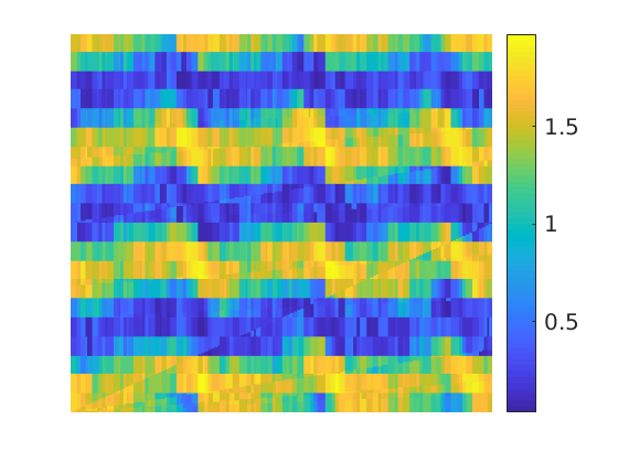
Figure 1: Coefficient $A$ (left) and errors (right) for example 1.

4.2 Example 2

In the second example, we choose ${\Gamma=\{x\in\partial\Omega\colon x_{1}=0\}}$, $f(x,t)=\sin(4\pi x_{1})(1-t)$ and $v_{0}=0$. We further let $u_{0}\in H^{1}_{\Gamma}$ be the solution of

$$a(u_{0},v)=\int_{\Omega}5\sin(\pi x_{1})\sin(\pi x_{2})v\,dx$$

for all $v\in H^{1}_{\Gamma}$. The coefficient $A$ is shown in Figure 2 (left), where $\alpha=1$, $\beta=17.78$ with $\varepsilon=0.02$. The precise formula for $A$ is

$$A(x)=1.9 \cdot\left(\lfloor 2x_{1}\rfloor\lfloor 8(1-x_{1})\rfloor+\lfloor 2(1-x_{1})\rfloor\lfloor 8x_{1}\rfloor\right)$$

$$\cdot\left(\lfloor 2x_{2}\rfloor\lfloor 8(1-x_{2})\rfloor+\lfloor 2(1-x_{2})\rfloor\lfloor 8x_{2}\rfloor\right)$$

$$\cdot\sin(\lfloor 32x_{1}\rfloor)^{2}\,\sin(\lfloor 64x_{2}\rfloor)^{2}+1.$$

The other discretization parameters are chosen as defined above. The red curve in Figure 2 (right) shows the errors of the standard method (3.3) with $\ell=2$ and the green curve shows the errors of the standard method with $\ell=4$. It can be seen that the red curve stagnates for smaller values of $H$ which is in accordance with the theoretical observations that $\ell$ needs to be chosen proportional to $|\log(H)|$. The convergence rate is again in line with the theoretical results and seems to be even slightly better for $\ell=4$ at around $1.5$. Note that, as in the first example, the errors of the simplified method based on (2.14) are very close to the errors of the standard method but are not depicted for better visibility. Also, since the value $\beta$ is only taken in a small part of the domain, the CFL condition can be slightly relaxed for this example.

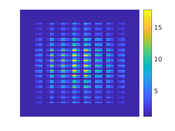
Figure 2: Coefficient $A$ (left) and errors (right) for example 2.

5 Conclusions

In this work, we have discussed a discretization of the wave equation with rough coefficients. We have used the LOD method in space and the explicit leapfrog scheme for the time discretization and are able to obtain first-order convergence under suitable assumptions on the initial data and subject to a relaxed version of the CFL condition. Numerical experiments illustrate the theoretical findings.

Ongoing research aims at further weakening the presented assumptions on the initial data especially in the context of $L^{2}(L^{2})$ error estimates and the generalization to elastic and poroelastic waves based on preparatory work [7, 3]. Additionally, the long-time behavior of numerical solutions to the wave equation will be considered.

References

- [1] A. Abdulle and M. J. Grote. Finite element heterogeneous multiscale method for the wave equation. Multiscale Model. Simul., 9(2):766–792, 2011.
- [2] A. Abdulle and P. Henning. Localized orthogonal decomposition method for the wave equation with a continuum of scales. Math. Comp., 86(304):549–587, 2017.
- [3] R. Altmann, E. Chung, R. Maier, D. Peterseim, and S.-M. Pun. Computational multiscale methods for linear heterogeneous poroelasticity. ArXiv e-prints, 1801.00615, 2018.
- [4] D. Arjmand and O. Runborg. Analysis of heterogeneous multiscale methods for long time wave propagation problems. Multiscale Model. Simul., 12(3):1135–1166, 2014.
- [5] Susanne C Brenner. Two-level additive Schwarz preconditioners for nonconforming finite elements. Contemporary Mathematics, 180:9–14, 1994.
- [6] F. Brezzi and M. Fortin. Mixed and hybrid finite element methods, volume 15. Springer Science & Business Media, 2012.
- [7] D. Brown and D. Gallistl. Multiscale sub-grid correction method for time-harmonic high-frequency elastodynamics with wavenumber explicit bounds. ArXiv e-prints, 1608.04243, 2016.
- [8] D. Brown, D. Gallistl, and D. Peterseim. Multiscale Petrov-Galerkin method for high-frequency heterogeneous Helmholtz equations. In Meshfree methods for partial differential equations VIII, volume 115 of Lect. Notes Comput. Sci. Eng., pages 85–115. Springer, 2017.
- [9] S. H. Christiansen. Foundations of finite element methods for wave equations of Maxwell type. In Applied wave mathematics, pages 335–393. Springer, 2009.
- [10] W. E and B. Engquist. The heterogeneous multi-scale method for homogenization problems. In Multiscale Methods in Science and Engineering, volume 44 of Lect. Notes Comput. Sci. Eng., pages 89–110. Springer, 2005.
- [11] W. E, B. Engquist, et al. The heterogeneous multiscale methods. Commun. Math. Sci., 1(1):87–132, 2003.
- [12] B. Engquist, H. Holst, and O. Runborg. Multi-scale methods for wave propagation in heterogeneous media. Commun. Math. Sci., 9(1):33–56, 2011.
- [13] B. Engquist, H. Holst, and O. Runborg. Multiscale methods for wave propagation in heterogeneous media over long time. In Numerical analysis of multiscale computations, volume 82 of Lect. Notes Comput. Sci. Eng., pages 167–186. Springer, 2012.
- [14] Alexandre Ern and Jean-Luc Guermond. Finite element quasi-interpolation and best approximation. ESAIM Math. Model. Numer. Anal., 51(4):1367–1385, 2017.
- [15] L. C. Evans. Partial Differential Equations. Graduate studies in mathematics. American Mathematical Society, 2010.
- [16] D. Gallistl and D. Peterseim. Stable multiscale Petrov-Galerkin finite element method for high frequency acoustic scattering. Comput. Methods Appl. Mech. Engrg., 295:1–17, 2015.
- [17] F. Hellman. Gridlod. https://github.com/fredrikhellman/gridlod, 2017. GitHub repository, commit 3e9cd20970581a32789aa1e21d7ff3f7e8f0b334.
- [18] P. Henning and D. Peterseim. Oversampling for the multiscale finite element method. Multiscale Model. Simul., 11(4):1149–1175, 2013.
- [19] P. Joly. Variational methods for time-dependent wave propagation problems. In Topics in computational wave propagation, volume 31 of Lect. Notes Comput. Sci. Eng., pages 201–264, Springer, 2003.
- [20] R. Kornhuber, D. Peterseim, and H. Yserentant. An analysis of a class of variational multiscale methods based on subspace decomposition. Math. Comp., 87:2765–2774, 2018.
- [21] R. Kornhuber and H. Yserentant. Numerical homogenization of elliptic multiscale problems by subspace decomposition. Multiscale Model. Simul., 14(3):1017–1036, 2016.
- [22] A. Mlqvist and D. Peterseim. Localization of elliptic multiscale problems. Math. Comp., 83(290):2583–2603, 2014.
- [23] Peter Oswald. On a BPX-preconditioner for P1 elements. Computing, 51(2):125–133, 1993.
- [24] H. Owhadi and L. Zhang. Numerical homogenization of the acoustic wave equations with a continuum of scales. Comput. Methods Appl. Mech. Engrg., 198(3-4):397–406, 2008.
- [25] H. Owhadi and L. Zhang. Gamblets for opening the complexity-bottleneck of implicit schemes for hyperbolic and parabolic ODEs/PDEs with rough coefficients. J. Comput. Phys., 347:99–128, 2017.
- [26] H. Owhadi, L. Zhang, and L. Berlyand. Polyharmonic homogenization, rough polyharmonic splines and sparse super-localization. ESAIM Math. Model. Numer. Anal., 48(2):517–552, 2014.
- [27] D. Peterseim. Variational multiscale stabilization and the exponential decay of fine-scale correctors. In Building bridges: connections and challenges in modern approaches to numerical partial differential equations, volume 114 of Lect. Notes Comput. Sci. Eng., pages 341–367. Springer, 2016.
- [28] D. Peterseim. Eliminating the pollution effect in Helmholtz problems by local subscale correction. Math. Comp., 86(305):1005–1036, 2017.
- [29] D. Peterseim and M. Schedensack. Relaxing the CFL condition for the wave equation on adaptive meshes. J. Sci. Comput., 72(3):1196–1213, 2017.