Statistical properties of Faraday rotation measure in external galaxies – I: intervening disc galaxies

Abstract

Deriving the Faraday rotation measure (RM) of quasar absorption line systems, which are tracers of high-redshift galaxies intervening background quasars, is a powerful tool for probing magnetic fields in distant galaxies. Statistically comparing the RM distributions of two quasar samples, with and without absorption line systems, allows one to infer magnetic field properties of the intervening galaxy population. Here, we have derived the analytical form of the probability distribution function (PDF) of RM produced by a single galaxy with an axisymmetric large-scale magnetic field. We then further determine the PDF of RM for one random sight line traversing each galaxy in a population with a large-scale magnetic field prescription. We find that the resulting PDF of RM is dominated by a Lorentzian with a width that is directly related to the mean axisymmetric large-scale field strength $\langle B_{0}\rangle$ of the galaxy population if the dispersion of $B_{0}$ within the population is smaller than $\langle B_{0}\rangle$. Provided that RMs produced by the intervening galaxies have been successfully isolated from other RM contributions along the line of sight, our simple model suggests that $\langle B_{0}\rangle$ in galaxies probed by quasar absorption line systems can be measured within $\approx 50$ per cent accuracy without additional constraints on the magneto-ionic medium properties of the galaxies. Finally, we discuss quasar sample selection criteria that are crucial to reliably interpret observations, and argue that within the limitations of the current database of absorption line systems, high-metallicity damped Lyman-$\alpha$ absorbers are best suited to study galactic dynamo action in distant disc galaxies.

1 Introduction

Magnetic fields in star-forming disc galaxies in the local Universe ($\lesssim 50$ Mpc) have been studied in detail, with most studies indicating the existence of a galactic dynamo (see Beck et al., 1996; Beck, 2016, for reviews). However, only a handful of studies exist to date on magnetic fields in high redshift ($z\gtrsim 0.1$) galaxies (e.g Kronberg et al., 1992; Oren & Wolfe, 1995; Bernet et al., 2008; Joshi & Chand, 2013; Farnes et al., 2014; Kim et al., 2016; Mao et al., 2017). The evolution of magnetic fields in disc galaxies over cosmological timescales has been studied through magnetohydrodynamic simulations (e.g. de Avillez & Breitschwerdt, 2005; Arshakian et al., 2009; Hanasz et al., 2009; Gent et al., 2013b, a; Chamandy et al., 2013; Burkhart et al., 2013; Pakmor et al., 2014; Rodrigues et al., 2015). These simulations have shown that fields on scales $\ll 1$ kpc can be amplified on a relatively short timescale (a few hundred Myrs) via a fluctuation dynamo (see e.g., Subramanian, 1999; Federrath et al., 2011). However, the amplification and ordering of fields on larger, $\gtrsim 1$ kpc, scales via a large-scale dynamo requires billions of years (e.g., Arshakian et al., 2009; Chamandy et al., 2013; Pakmor et al., 2014). Observational constraints on the amplification timescale of the large-scale magnetic fields in galaxies are lacking and therefore, the evolution of magnetic fields in galaxies still remains an important open question in astronomy.

Directly mapping the magnetic field structure and strength in high-$z$ galaxies, as has been done for nearby galaxies, will be a challenging proposition even for next-generation radio telescopes like the Square Kilometre Array (SKA) and its pathfinders. However, advances have been made in inferring the strength of magnetic fields through statistical studies of excess Faraday rotation measure (RM) introduced by a sample of intervening galaxies when observed against background polarized quasars (see, e.g., Oren & Wolfe, 1995; Bernet et al., 2008; Bernet et al., 2013) — the so-called “backlit-experiment”. Intervening galaxies are identified through the presence of absorption lines at a redshift significantly lower than that of the quasar. Since RM is the integral of the magnetic field component weighted by the free electron density along the entire line of sight, such studies are faced with the challenge of disentangling the combined RM of the quasar itself, the intergalactic medium (IGM) and the Milky Way, from the RM originating in the interstellar medium (ISM) of the intervening galaxy. The first three terms can be statistically estimated by measuring the RM towards a sample of quasars without intervening absorption lines. Comparing the RMs of quasar samples with intervening absorption with those without intervening absorption then allows one to statistically determine the excess RM produced by the intervening galaxies. We emphasize that this approach only allows one to study statistical properties of magnetic fields in a sample of high-$z$ galaxies.

To study magnetic fields in individual distant galaxies, Mao et al. (2017) made use of gravitational lensing of a polarized background quasar lensed by a foreground galaxy. The authors inferred the large-scale magnetic field properties in a galaxy at $z=0.439$. The RM contributions by the quasar, the IGM, and the Milky Way are approximately the same for the lensed images of the quasar. Therefore, by comparing the RMs of the lensed images, it is possible to measure the magnetic field strength and geometry in the intervening galaxy. Suitable sightlines for such studies, with a foreground galaxy lensing a background polarized radio-loud quasar, is limited at present. Further, known radio-bright lens systems mostly have $\sim$arcsecond-scale image separations, i.e. to lensing galaxies at the upper end of the galaxy mass function with halo masses $\gtrsim 10^{10}~{}\rm M_{\odot}$. Hence, in order to trace the cosmic evolution of magnetic fields across a wide range of galaxy types, including lower mass galaxies that are believed to dominate the galaxy population at early cosmic times, statistical backlit approaches are needed.

In this paper, we first derive an analytical expression of the probability distribution function (PDF) of the RM for a galaxy with an axisymmetric large-scale magnetic field when viewed at an arbitrary inclination. To enable the derivation of the analytical solution for the PDF of the RM, we have adopted a simple set of assumptions for the magneto-ionic medium of the target galaxies. The analytical solutions allow one to explore the dependence of the PDF of the RM on various magnetic field parameters, and thereby understand how realistic, often more complicated, assumptions can affect the inferred field properties. Using the analytical expression we gain insights into the distribution of RMs measured along lines of sight passing through a sample of disc galaxies with random distributions of inclination angle, radius and azimuthal angle of intersection, strength and pitch angle of the magnetic field, and free electron density.

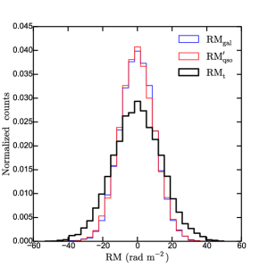
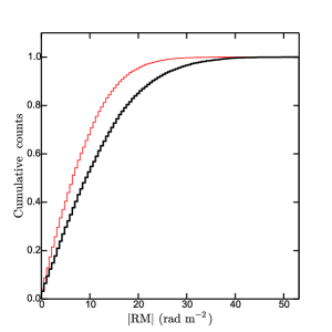
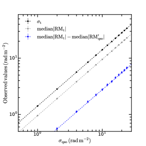
Figure 1: Left: Distribution of ${\rm RM_{t}}={\rm RM_{gal}}+{\rm RM_{qso}^{\prime}}$ (black histogram), where ${\rm RM_{gal}}$ (blue histogram) and $\rm RM_{qso}^{\prime}$ (red histogram) are Gaussian random variables with zero mean and $\sigma=10$ rad m^-2. Middle: Cumulative distributions of $|{\rm RM_{t}}|$ (in black) and $|{\rm RM_{qso}^{\prime}}|$ (in red). Right: Variation of the observed quantities as a function of the $\sigma_{\rm qso}$ assuming both ${\rm RM_{gal}}$ and $\rm RM_{qso}^{\prime}$ follow the same Gaussian distributions.

In Section 2, we describe the general setup for a backlit-experiment that one uses to derive the RMs of high-redshift galaxies. We identify three sources of bias in traditional analyses that can give rise to ambiguity in the measured magnetic field strengths. In Section 3, we present the methodology and assumptions used in this paper. For simplicity, we only consider magnetic field in galactic discs. The properties of the PDF of the RM for an intervening galaxy and that for a sample of intervening galaxies are presented in Section 4. We describe in Section 5 the selection criteria of target absorber sample that satisfies the assumptions we have made. We discuss future work necessary towards a complete understanding of the evolution of magnetic fields in galaxies in Section 6, and summarize our results in Section 7.

2 The data and various pitfalls in the analysis

The presence of a galaxy along, or close to, the line of sight to a background quasar can be deduced from the presence of “damped” or “sub-damped” neutral hydrogen Lyman-$\alpha$ absorption or strong metal-line absorption (arising from transitions in Mgii, Feii, Siii, etc.) imprinted on the optical and/or ultraviolet (UV) spectra of the quasar. Damped Lyman-$\alpha$ absorbers (DLAs) are the highest neutral hydrogen (Hi) column density absorbers in quasar absorption spectra, with Hi column densities $\geq 2\times 10^{20}$ cm^-2, and are believed to arise from sightlines passing through galaxy discs (e.g. Wolfe et al., 2005). Sub-DLAs have somewhat lower Hi column densities, $\approx 10^{19}-10^{20}$ cm^-2, and along with Lyman-limit systems and most strong metal-line absorbers, are likely to mostly arise in the circumgalactic medium (CGM; e.g. Zibetti et al., 2007; Nestor et al., 2007; Neeleman et al., 2016). Today, the largest absorber samples have been obtained from searches through quasar absorption spectra from the Sloan Digital Sky Survey (SDSS) (e.g. Prochaska et al., 2005; Noterdaeme et al., 2009; Noterdaeme et al., 2012; Zhu & Ménard, 2013), with $\gtrsim 10,000$ DLAs currently known at $z\gtrsim 2$ (e.g. Noterdaeme et al., 2012) and $\gtrsim 40,000$ strong Mgii absorbers known at $z\gtrsim 0.4$ (e.g. Zhu & Ménard, 2013). The sample of quasars with foreground absorbing galaxies will henceforth be referred to as the “target” sample. We emphasize that our aim is to determine the magnetic fields of the intervening absorber galaxies, and that the quasars are used only as background torches.

The net RM (${\rm RM_{t}}$) of the background quasar and the absorption system in the observer’s frame for a single line of sight is given by,

$${\rm RM_{t}}=\dfrac{{\rm RM_{gal}}}{(1+z_{\rm gal})^{2}}+\dfrac{{\rm RM_{qso}}}{(1+z_{\rm qso})^{2}}+\Delta_{\rm RM}.$$ (1)

Here, $\rm RM_{gal}$ and $\rm RM_{qso}$ are the RM of the foreground absorber galaxy and the intrinsic RM of the background quasar in their rest frames, respectively, and $z_{\rm gal}$ and $z_{\rm qso}$ are their redshifts. $\Delta_{\rm RM}$ is the additional contributions to the RM along the line of sight and is defined as $\rm\Delta_{RM}=RM_{IGM}+RM_{MW}+\delta_{\rm RM}$, where $\rm RM_{IGM}$ and $\rm RM_{MW}$ are the contributions from the IGM and the Milky Way, respectively, and $\delta_{\rm RM}$ is the measurement noise. We define $\rm RM_{qso}^{\prime}={\rm RM_{qso}}\,{(1+{z_{\rm qso}})^{-2}}+\Delta_{\rm RM}$, as the RM that would have been measured towards the quasar in the absence of the intervening galaxy; thus, ${\rm RM_{t}}={\rm RM_{gal}}\,(1+z_{\rm gal})^{-2}+{\rm RM_{qso}^{\prime}}$.

It is not possible to determine ${\rm RM_{gal}}$ from a single measurement of ${\rm RM_{t}}$, and therefore measurements along lines of sight towards quasars without intervening absorbers are required to statistically infer $\rm RM_{qso}^{\prime}$. These can be compared with the measurement of ${\rm RM_{t}}$ towards quasar sightlines with absorbing galaxies to estimate the statistical properties of ${\rm RM_{gal}}$, and to subsequently derive the strength of the magnetic field in the absorber galaxy. The sample of quasars without foreground absorber galaxies, which are used to estimate $\rm RM_{qso}^{\prime}$, are referred to as the “control” sample. The RM values of the quasars in the control sample are given by,

$${\rm RM_{c}}=\dfrac{\rm RM_{qso,c}}{(1+z_{\rm qso,c})^{2}}+\Delta_{\rm RM}.$$ (2)

In order to infer ${\rm RM_{gal}}$ produced by the absorber galaxies in our target sample, we will assume that ${\rm RM_{c}}$ and $\rm RM_{qso}^{\prime}$ have the same statistical properties. Thus, a comparison between the distributions of ${\rm RM_{t}}$ and ${\rm RM_{c}}$ would then yield the excess contribution from ${\rm RM_{gal}}\,{(1+z_{\rm gal})^{-2}}$ in the former quantity.

When interpreting the distribution of ${\rm RM_{t}}$, it is important to consider the effects of each of the variables, i.e., $\rm RM_{gal}$, $\rm RM_{qso}$, $\rm RM_{qso,c}$, $\Delta_{\rm RM}$, $z_{\rm gal}$, $z_{\rm qso}$, and $z_{\rm qso,c}$, where subscript ‘c’ refers to the control sample. In the following, we discuss the potential sources of bias that are introduced by standard analysis procedures used in the literature to date. In Table 2, we list and describe in brief the variables and notations used in this paper and in the literature.

We note, that the distribution of ${\rm RM_{t}}$ is the convolution of the distributions of the terms, ${\rm RM_{gal}}\,(1+{z_{\rm gal}})^{-2}$ and $\rm RM_{qso}^{\prime}$, in Eq. (1), i.e., $\mathrm{PDF}({\rm RM_{t}})=\mathrm{PDF}\left({\rm RM_{gal}}\,(1+{z_{\rm gal}})^{-2}\right)\otimes\mathrm{PDF}\left(\rm RM_{qso}^{\prime}\right)$. Therefore, a formal approach to study the distribution of ${\rm RM_{gal}}$ is to deconvolve the distribution of $\rm RM_{qso}^{\prime}$ (using the distribution of ${\rm RM_{c}}$ as its proxy), from that of ${\rm RM_{t}}$. Unfortunately, we do not a priori know the distributions of ${\rm RM_{t}}$ and ${\rm RM_{c}}$, and there is no formal mathematical procedure in the literature to perform a deconvolution on arbitrary statistical distributions. One hence usually simply compares the distributions of ${\rm RM_{t}}$ and ${\rm RM_{c}}$ to test whether or not the contribution from ${\rm RM_{gal}}$ produces a statistical difference between the two distributions. It is beyond the scope of this paper to investigate a formal deconvolution method, and how such a procedure might affect the results. In this work, we study the properties of the distribution of ${\rm RM_{gal}}$ through simulations, and how this distribution is related to the strength of the large-scale magnetic fields in high-$z$ galaxies.

2.1 The bias from using $|\rm RM|$

To determine the contribution of ${\rm RM_{gal}}$ to ${\rm RM_{t}}$, the empirical cumulative distribution function (CDF) of $|{\rm RM_{t}}|$ has been compared to that of $|{\rm RM_{c}}|$ in the past (see, e.g., Bernet et al., 2008; Farnes et al., 2014). The difference in their median values has been used to estimate the magnetic field strengths (e.g., Farnes et al., 2014). In this section, we demonstrate that using the absolute value of RM, rather than the value of RM itself, introduces a systematic bias in the results.

To demonstrate this, we consider the simple case where ${z_{\rm gal}}\approx 0$, so that ${\rm RM_{t}}={\rm RM_{gal}}+\rm RM_{qso}^{\prime}$. We assume Gaussian random distributions for both ${\rm RM_{gal}}$ and $\rm RM_{qso}^{\prime}$, i.e. their PDFs are, respectively, given by $X=\mathcal{N}\left(\langle{\rm RM_{gal}}\rangle,\sigma_{\rm gal}\right)$ and $Y=\mathcal{N}\left(\langle\rm RM_{qso}^{\prime}\rangle,\sigma_{\rm qso}\right)$. This is equivalent to the case where the probability distribution of ${\rm RM_{gal}}\,(1+{z_{\rm gal}})^{-2}$ is Gaussian. In this case, the PDF of the sum $X+Y$ is the convolution of the two PDFs and is given by $X+Y=\mathcal{N}\left(\langle{\rm RM_{gal}}\rangle,\sigma_{\rm gal}\right)\otimes\mathcal{N}\left(\langle\rm RM_{qso}^{\prime}\rangle,\sigma_{\rm qso}\right)=\mathcal{N}\left(\langle{\rm RM_{gal}}\rangle+\langle\rm RM_{qso}^{\prime}\rangle,\sqrt{\sigma_{\rm gal}^{2}+\sigma_{\rm qso}^{2}}\right)$. We emphasize that the statistical properties of $|X+Y|$ are very different, and significantly more complicated, than those of $X+Y$. The absolute value of a Gaussian is known as the folded normal distribution. The median, mean and variance of this distribution cannot be written in closed form, unless the mean is zero, and its shape is determined by both its mean and variance.

We find that the difference between the median values of $|{\rm RM_{t}}|$ and $|\rm RM_{qso}^{\prime}|$ increases with increasing $\sigma_{\rm qso}$. In Fig. 1 (left panel), we simulate the distributions of ${\rm RM_{t}}$, ${\rm RM_{gal}}$ and $\rm RM_{qso}^{\prime}$. We consider similar Gaussian distributions for ${\rm RM_{gal}}$ and $\rm RM_{qso}^{\prime}$ with zero mean and the same dispersion $\sigma_{\rm gal}=\sigma_{\rm qso}$. For such a case, $\langle{\rm RM_{t}}\rangle=\langle{\rm RM_{gal}}\rangle+\langle\rm RM_{qso}^{\prime}\rangle=0$ rad m^-2, and the observed dispersion of ${\rm RM_{t}}$ ($\sigma_{\rm t}$) is given by $\sigma_{\rm t}^{2}=\sigma_{\rm gal}^{2}+\sigma_{\rm qso}^{2}$. However, if we compare the absolute values of ${\rm RM_{t}}$ and $\rm RM_{qso}^{\prime}$ (as shown in the middle panel of Fig. 1), we find that the CDFs are different, such that the median value of $|{\rm RM_{t}}|$ is greater than the median value of $|\rm RM_{qso}^{\prime}|$. Such a difference in the CDF of $|\rm RM|$ between the target and control samples has been interpreted in the past as implying that intervening galaxies show excess median RM and has been used to derive the strength of the large-scale field (Farnes et al., 2014). Our simulated data indicate that such a difference in the CDFs may simply arise from the increased dispersion in the RM of sightlines that host an intervening galaxy, and does not necessarily imply an excess in median value of RM originating from large-scale fields in the absorbers.

Figure 1 (right panel) shows how the inferred difference of the statistics of absolute RM values varies as a function of $\sigma_{\rm qso}$ (which is the same as $\sigma_{\rm gal}$ in this example). The black points show the dispersion of the observed RM, $\sigma_{\rm t}$; this is related to $\sigma_{\rm qso}$ as $\sigma_{\rm t}=\sqrt{2}\,\sigma_{\rm qso}$ in this example. The grey points show how the median value of $|{\rm RM_{t}}|$ varies as a function of $\sigma_{\rm qso}$. Clearly, the median value of $|{\rm RM_{t}}|$ has a linear relation with $\sigma_{\rm qso}$, whereas the median value of ${\rm RM_{t}}$ is zero. The blue points show the variation of the difference between the median values of $|{\rm RM_{t}}|$ and $|\rm RM_{qso}^{\prime}|$. This difference is just an artefact of the increased dispersion, and does not necessarily imply a true difference between the medians of the two population. For $\sigma_{\rm qso}\sim 6\text{--}7$ rad m^-2 (Schnitzeler, 2010; Oppermann et al., 2015), a typical value for the dispersion of the RM of extragalactic sources in the observer’s frame, the difference of medians can be up to $\sim 2$ rad m^-2. This is a significant fraction of the differences in median $|\rm RM|$ reported earlier in studies based on Mgii absorption systems (e.g. Farnes et al., 2014). Using $|\rm RM|$ instead of RM introduces a similar bias also for other choices of the means and variances of ${\rm RM_{gal}}$, $\rm RM_{qso}^{\prime}$ and ${\rm RM_{c}}$. Therefore we believe, RM, rather than $\rm|RM|$, is perhaps a better quantity to compare between the target and the control sample to infer the magnetic field properties of the intervening galaxies.

2.2 The redshift bias

A comparison between the distributions of RM of the target and control sample, ${\rm RM_{t}}$ and ${\rm RM_{c}}$, is only meaningful if the distributions of ${\rm RM_{c}}$ and $\rm RM_{qso}^{\prime}$ are similar. For this, a comparison between Eqs. (1) and (2) shows that quasars in the target and control samples should be selected in such a way that ${\rm RM_{qso}}\,(1+{z_{\rm qso}})^{-2}$ and ${\rm RM_{qso,c}}\,(1+z_{\rm qso,c})^{-2}$ follow similar statistical distribution. Even if ${\rm RM_{qso}}$ and $\rm RM_{qso,c}$ follow the same distribution, a difference in the redshift distributions of the target and control samples can introduce a systematic bias, due to the $(1+z)^{-2}$ factor in the expression for RM in the observer’s frame. In fact, in such a situation, the contribution of $\rm RM_{IGM}$ in the $\Delta_{\rm RM}$ term will also be different for the two sets of lines of sight, introducing additional bias (e.g. Akahori et al., 2016).

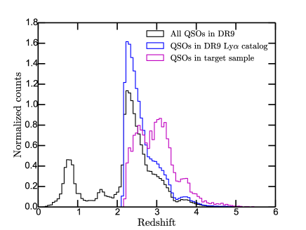
Figure 2: Redshift distribution of the quasars in the SDSS DR9 catalog are shown as the black histogram and for background quasars in the target DLA sample as the magenta histogram. Blue histogram show the redshift distribution of quasars in the BOSS Lyman-$\alpha$ forest catalog.

Here, we assess the systematic bias produced by different redshift distributions of the quasars in the target and the control samples, using DLAs as the intervening galaxies. Fig. 2 shows the redshift distribution of various quasar sub-samples drawn from the SDSS DR9 catalogue (Ahn et al., 2012). The redshift distribution of all quasars in the SDSS DR9 catalog (Pâris et al., 2012) is shown in black. The redshift distribution of the quasars in the BOSS Lyman-$\alpha$ forest sample from the SDSS DR9 (Lee et al., 2013) is shown in blue, while that of SDSS DR9 quasars with foreground DLAs (Noterdaeme et al., 2012; Lee et al., 2013) is shown in magenta. Thus, the quasars in the control sample have $z_{\rm qso,c}\approx 0.5-4$, while those in the target sample have ${z_{\rm qso}}\approx 2-4$. It is clear that a simple use of the full SDSS DR9 quasar catalogue (i.e. without redshift cuts to ensure similar quasar redshift distributions in the target and control samples) to select polarized quasars for studies of intervening galaxies identified as DLAs would yield $\langle{z_{\rm qso}}\rangle\gtrsim\langle z_{\rm qso,c}\rangle$.

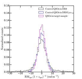
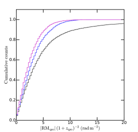
Figure 3: Top: Distribution of ${\rm RM_{qso}}\,(1+{z_{\rm qso}})^{-2}$ for different redshift coverages given in Fig. 2. Bottom: Cumulative distribution of $|{\rm RM_{qso}}|\,(1+{z_{\rm qso}})^{-2}$. We assume that the intrinsic (rest-frame) RMs of the quasars follow a Gaussian distribution with zero mean and a standard deviation of $50\,\rm rad\,m^{-2}$. The distribution in black is for control quasars chosen from the entire SDSS DR9 catalog, blue is for control quasars chosen from BOSS Lyman-$\alpha$ forest catalog and magenta is for quasars in the target DLA sample.

The top and bottom panels of Fig. 3 show the effect of different redshift distributions for the control and target quasar samples on the PDF of RM${}_{\rm qso}(1+z_{\rm qso})^{-2}$ (top panel) and the CDF of $|{\rm RM_{qso}}|(1+z_{\rm qso})^{-2}$ (bottom panel). Here, we have assumed that quasars at all redshifts have an intrinsic RM distribution with zero mean and $\sigma_{\rm qso}=50$ rad m^-2 in their rest-frame. Since $(1+{z_{\rm qso}})^{-2}$ is non-linear in ${z_{\rm qso}}$, the distribution of ${\rm RM_{t}}$ is non-Gaussian. If we do not impose redshift constraints on the control and target samples, the redshifts of the control and target samples would be drawn from the distributions shown, respectively, in black and magenta in Fig. 2. This implies that the control sample can have $\sigma_{\rm qso}$ up to $\approx 5$ rad m^-2 larger than that of the target sample in the observer’s frame (comparing the black and magenta histograms in the top panel of Fig. 3). This would yield a median value of $|{\rm RM_{c}}|$ lower by $\approx 1.5$ rad m^-2 than the median value of $|\rm RM_{qso}^{\prime}|$.

The above differences can be mitigated if the quasars of the control and target samples are chosen to have the same redshift distribution. In the case of the SDSS DR9, it would appear that this might be achieved by selecting both the control and the target quasars from the BOSS Lyman-$\alpha$ forest sample, i.e., the redshift distribution shown in blue in Fig. 2. We note, however, that such a selection from the BOSS catalogue actually does not yield similar statistical distributions of ${\rm RM_{c}}$ and $\rm RM_{qso}^{\prime}$ (see the blue and magenta curves in Fig. 3), despite similar range of their redshift coverage. The difference arises due to the differences in the actual redshift distributions of the quasars of the two samples (see the blue and magenta curves in Fig. 2), as the redshift distribution of quasars in the target sample contains an additional dependence on the probability of finding an absorbing galaxy at a given redshift. It is hence critical to carry out statistical tests to ensure statistically identical redshift distributions for the radio-bright quasars in the target and the control samples.

2.3 Bias from incomplete absorber redshift coverage

An additional bias arises due to the restricted wavelength coverage of the spectrographs used for the absorption surveys, which implies that they are only sensitive to absorbers lying in a limited redshift range. For example, ground-based optical surveys for DLAs are sensitive to Lyman-$\alpha$ absorption only at $z\gtrsim 1.7$, even when using UV-sensitive spectrographs; the SDSS is only sensitive to DLAs at $z\gtrsim 2$ (e.g. Noterdaeme et al., 2012). However, the redshift line number density of DLAs is $\approx 0.25$ per unit redshift at $z\gtrsim 2$ (Prochaska et al., 2005), and $\approx 0.1$ per unit redshift at $z\approx 1$ (Rao et al., 2006). This implies that it is not trivial to generate a “clean” high-redshift quasar control sample from a survey such as the SDSS DR9, because there is $\approx 25$ per cent probability that a quasar at $z>2$ would have an absorbing galaxy at $z<2$ that is undetected simply because the relevant wavelength range has not been covered in the survey.

The $(1+z)^{-2}$ dilution of the rest-frame ${\rm RM_{gal}}$ makes this a serious issue, because the RM contribution in the observer’s frame from an absorber at $z\lesssim 1$ is significantly larger (typically by factor $\sim 2\text{--}4$) than that at $z\gtrsim 2$. The presence of a DLA at $z\lesssim 1$ towards a high-$z$ quasar would imply a higher $|\rm RM|$ than if the DLA were absent.

The effect of such putative undetected absorbers on the derived distribution of ${\rm RM_{t}}$ depends critically on the redshift distributions of the target and the control quasar samples. For the simple SDSS DR9 case discussed in the previous section, where the quasar control sample has a lower median redshift, quasars in the target sample are more likely to have undetected absorbers at low redshifts, and should hence have, statistically, a higher ${\rm RM_{t}}$ than the quasars of the control sample. If this effect is not corrected for, it would yield higher ${\rm RM_{gal}}$ values for the DLAs in the sample than the true ones. We note that this bias goes in the opposite direction as the bias discussed in the previous section.

The best way to remove this bias is again to ensure that the target and control quasar samples have the same redshift distribution. If so, the issue of undetected absorbers at low redshifts should affect the quasars of both the target and the control samples in the same manner, implying no systematic bias in the derived ${\rm RM_{gal}}$ values for the target sample.

3 Basic equations

As discussed earlier, our approach to estimating the large-scale magnetic field is based on RM measurements towards a large number of quasars with foreground absorbers; the RM estimates contain information on the magnetic field component along the line of sight for each intervening galaxy. Since $|\rm RM|$ introduces a systematic bias (Section 2.1), one should work directly with the distribution of RM. In this section, we derive an analytical form of the PDF of the RM for an intervening disc galaxy with an axisymmetric spiral magnetic field geometry, observed along random lines of sight through the disc. This will be used to infer the magnetic field properties of high-$z$ disc galaxies from the observed RM distribution.

Note that we will, in later sections, focus on the properties of the distribution of the RM originating only from the large-scale fields in the intervening galaxies in their rest frame. This is equivalent to the case — in an observed backlit-experiment — that the contribution of RM from the quasar, the IGM, the Milky Way and noise, i.e. $\rm RM_{qso}^{\prime}$, is either negligible compared to the observed RM or ${\rm RM_{gal}}$ has already been isolated from the contribution of $\rm RM_{qso}^{\prime}$ (see the discussion in Section 2).

3.1 Assumptions on the Faraday rotating medium

We model an intervening galaxy as a disc with an axisymmetric spiral magnetic field and a radially decreasing free electron density ($n_{\rm e}$). We assume that the amplitude and geometry of the magnetic field, as well as the electron density, do not vary with distance from the mid-plane of the galaxy. Faraday rotation in galaxies is produced from both turbulent and large-scale magnetic fields. The distribution of RM due to isotropic turbulent fields is expected to be a Gaussian with zero mean and its standard deviation is a measure of the strength of the turbulent field (see Section 5.2.1). Thus, for characterizing turbulent magnetic fields the dispersion of observed RM is sufficient. Since we are interested in studying the properties of RM produced by large-scale fields, we will work under the assumption that the RM originating from turbulent magnetic fields is insignificant within the three-dimensional illumination beam passing through the magneto-ionic medium of the galaxy. This can be achieved when the spatial extent of the polarized emission from the background quasar, as seen by the foreground galaxy, is large enough to encompass several turbulent cells, but small enough so that the RM contributed by the large-scale field does not vary significantly across the beam (see Section 5.2.1).

The magnetic field component along the line of sight ($B_{\|}$) at each point in a galaxy can be calculated via (e.g. Berkhuijsen et al., 1997),

$$B_{\|}=-(B_{r}\sin\theta+B_{\theta}\cos\theta)\sin i+B_{z}\cos i\;.$$ (3)

Here, $B_{r}$ and $B_{\theta}$ are, respectively, the radial and azimuthal components of the magnetic field, $\theta$ is the azimuthal angle, and $i$ is the inclination angle with respect to the plane of the sky. For an axisymmetric spiral magnetic field the pitch angle is defined as, $p=\arctan\left(B_{r}/B_{\theta}\right)$. $B_{z}$ is the magnetic field component perpendicular to the disc. In this paper we assume that $B_{z}=0$, to simplify our calculations, as it is significantly smaller in magnitude than $B_{r}$ and $B_{\theta}$ (Mao et al., 2010; Chamandy, 2016).

We assume that the total large-scale magnetic field ($B=\sqrt{B_{r}^{2}+B_{\theta}^{2}}$) varies exponentially with radius $r$ (e.g. Beck, 2007, 2015), such that, $B(r)=B_{\rm 0}\,{\rm e}^{-r/r_{B}}$, where $r_{B}$ is the radial scale-length and $B_{0}$ is the large-scale field strength at the centre of the galaxy. The radial scale-length of the ordered magnetic field in spiral galaxies is typically $\approx 15-25$ kpc (Beck, 2015; Berkhuijsen et al., 2016); we hence adopt $r_{B}=20$ kpc.

The radial variation of $n_{\rm e}$ is modelled as $n_{\rm e}(r)=n_{0}\,{\rm e}^{-r/r_{\rm e}}$. Here, $n_{0}$ is the electron density at the centre of the galaxy and $r_{\rm e}$ is the radial scale-length. We assume that $n_{\rm e}$ does not vary with distance from the midplane, and that the electrons are in a thick disc of uniform thickness, $h_{\rm ion}=500$ pc, centred at the midplane. For a sightline of inclination angle $i$ with respect to the plane of the sky, the path length through the disc is then $L=h_{\mathrm{ion}}/\cos i$. Finally, according to the NE2001 model (Cordes & Lazio, 2002), the ionized thick disc of the Milky Way shows a gradual decrease of $n_{\rm e}$ with Galactocentric radius, with $r_{\rm e}\gtrsim 15$ kpc, i.e. comparable to $r_{B}$. We hence adopt $r_{\rm e}\approx r_{B}\approx 20$ kpc for our calculations.

With these assumptions, the RM can be written as,

$$\begin{split}\mathrm{RM}&=0.81\,\left(\dfrac{\langle n_{\rm e}\rangle}{\rm cm^{-3}}\right)\,\left(\dfrac{\langle B_{\parallel}\rangle}{\rm\mu G}\right)\,\left(\dfrac{L}{\rm pc}\right)~{}{\rm rad\,m^{-2}}\\ &=-0.81\,n_{0}\,B_{0}\,{\rm e}^{-r/r_{0}^{\prime}}\,\cos(\theta-p)\,h_{\mathrm{ion}}\tan i\;,\end{split}$$ (4)

where $1/r_{0}^{\prime}=1/r_{B}+1/r_{\rm e}$.

3.2 Line of sight approximation

To calculate $B_{\|}$ and RM along a single line of sight, we have used a constant value of $B_{\|}$, $n_{\rm e}$ and $\theta$ throughout the ionized medium of the galactic disc that gives rise to Faraday rotation. This allows us to compute analytical solutions for the quantities of interest. Strictly speaking, such a simplification is inadequate for an inclined disc. Sightlines with $i\lesssim 45^{\circ}$ probe relatively narrow ranges of both galactocentric radii and $B$ values. For example, for our assumed $h_{\rm ion}=500$ pc and $r_{B}\approx 20$ kpc, and sightlines with $i\lesssim 45^{\circ}$, $B$ varies by less than $2$ per cent at the near and the far sides of the disc, with respect to its value at the mid-plane, while $\theta$ varies by less than $1.5^{\circ}$. Such small variations will not significantly affect our derived values of RM and subsequent results.

At higher inclinations, e.g. $i\approx 75^{\circ}$, $B$ varies by $\lesssim 10$ per cent along the sightline, and $\theta$ by $\lesssim 5^{\circ}$. This will affect the estimated values of RM at $\lesssim 15$ per cent level. At even larger inclinations $i>75^{\circ}$, while the errors due to the assumptions of constant $B$ and $\theta$ will be significant ($>20$ per cent), the probability of finding a galaxy-quasar pair will also be low, as the projected area of the galaxy on the sky is low for high $i$. Only a small fraction of the sightlines in the target sample would hence be at such high inclinations, implying that our approximations are unlikely to significantly affect the final results.

We note, that the inclination angle does not have a marked effect on $B$ primarily because $r_{B}\gg h_{\rm ion}$, and therefore the magneto-ionic disc essentially behaves like a thin disc. Similarly, because $r_{\rm e}$ is large, the variation of $n_{\rm e}$ through the disc at a particular radius is small. Overall, our simplifications will affect the derived values of RM at $\lesssim 15$ per cent for the extreme case, where the galaxy is inclined at $\approx 75^{\circ}$.

3.3 Distribution functions of the random parameters: azimuthal angle, inclination angle and impact radius

The quasar sightlines can intersect the intervening galaxies at any impact radius, inclination angle, and azimuthal angle. To model this, we assume uniform distributions for $\theta$ and $i$ where all values are equally likely, i.e., the probability densities have the form,

$$f_{\Theta}(\theta)=\begin{cases}~{}\dfrac{1}{2\pi},&\text{for }0\leq i\leq{2\pi},\\ ~{}0,&\text{otherwise. }\end{cases}$$ (5)

$$f_{I}(i)=\begin{cases}~{}\dfrac{2}{\pi},&\text{for }0\leq i\leq\dfrac{\pi}{2},\\ ~{}0,&\text{otherwise. }\end{cases}$$ (6)

We note, however, that the distribution of $i$ may not be strictly uniform even for the case of random lines of sight, with no preferred inclination angles of the intervening galaxy with respect to the observer and the background quasar. This is due to two competing reasons. On one hand, the probability of having a quasar behind a highly inclined galaxy is lower as such a galaxy would have a far smaller projected area in the plane of the sky than a relatively face-on galaxy. In Appendix B.3, we discuss how this may affect our results. On the other hand, for galaxies selected through absorption, the inclination angle and radius of intersection are related because, at large impact radii, a sightline through a highly inclined galaxy could yield a higher Hi column density and hence stronger absorption compared to a face-on galaxy. Modelling these effects simultaneously is difficult due to the lack of a large sample of absorber galaxies with information on the impact radii, the column density of the absorbing gas, and the inclination angle (see e.g. Kacprzak et al., 2011).

3.3.1 Distribution function of the impact radius

The projected distance between the background quasar and the center of the absorbing object, known as the impact parameter, is used to quantify the distance at which the line of sight intersects an absorber galaxy. For simplicity, we use the deprojected radial distance from the centre, $r$, instead of the impact parameter in this study. Using the radius in our calculations has the advantage of modelling the variations of physical parameters relatively easily. In contrast, the impact parameter depends on both the radii of impact and the inclination angle.

In general, we assume that a particular species of absorption line probes the radius range $R_{\rm min}\leq r\leq R_{\rm max}$ in the intervening galaxies. For example, $R_{\rm max}$ can be the transition radius at which the Hi column densities drop below the DLA threshold column density of $2\times 10^{20}$ cm^-2 (Wolfe et al., 2005). Or, for Mgii absorbers, it could be the radius at which the Mgii$\lambda$2796Å rest equivalent width falls below a threshold width (e.g. 0.5 Å; Rao et al., 2006). For the distribution of $r$, we assume the following two cases:

• Case 1: For a sample of galaxies, the probability of finding a background quasar at a radius $r$ within the range $r\pm\Delta r/2$ increases as $r\,\Delta r$. However, for an absorption selected sample of intervening galaxies, due to inclination effects such a linear behaviour with $r$ can be different and therefore we assume that the probability of finding a quasar at a radius $r$ scales as $r^{\eta}$ where $\eta$ could lie between 0 and 2. Since the absorber species probes up to a maximum radius $R_{\rm max}$, we truncate the $r^{\eta}$ function with an exponential of the form ${\rm e}^{-(r/R_{\rm max})^{6}}$. In this case, the PDF of $r$ is described by,

  $$f_{R}(r)=\dfrac{6}{R_{\rm max}^{\eta+1}\,\Gamma\left(\dfrac{\eta+1}{6}\right)}\,r^{\eta}\,{\rm e}^{-(r/R_{\rm max})^{6}},~{}~{}~{}0<r<\infty.$$ (7)

  The PDF $f_{R}(r)$ is shown in Fig. 4 for different values of $\eta$. It can easily be shown that, for the case where $r$ has a minimum radius $R_{\rm min}$, the $R_{\rm max}^{\eta+1}$ term in the denominator is replaced by $R_{\rm max}^{\eta+1}-R_{\rm min}^{\eta+1}$ and the gamma function is modified to $\Gamma\left({(\eta+1)}/{6},{R_{\rm min}^{6}}/{R_{\rm max}^{6}}\right)$. For $R_{\rm min}\ll R_{\rm max}$, $\Gamma\left({(\eta+1)}/{6},{R_{\rm min}^{6}}/{R_{\rm max}^{6}}\right)\approx\Gamma\left({(\eta+1)}/{6},0\right)$ and $R_{\rm max}^{\eta+1}-R_{\rm min}^{\eta+1}\approx R_{\rm max}^{\eta+1}$. Hence, we do not additionally invoke a $R_{\rm min}$.

• Case 2: It is plausible that the database of absorption line samples is incomplete in terms of the range of radii probed by the background quasars. To account for such a situation, we consider a simplified scenario where the radii at which the background quasars probe the absorber galaxies are uniformly distributed:

  $$f_{R}(r)=\begin{cases}~{}\dfrac{1}{R_{\rm max}-R_{\rm min}},&\text{for }R_{\rm min}\leq r\leq R_{\rm max},\\ ~{}0,&\text{otherwise. }\end{cases}$$ (8)

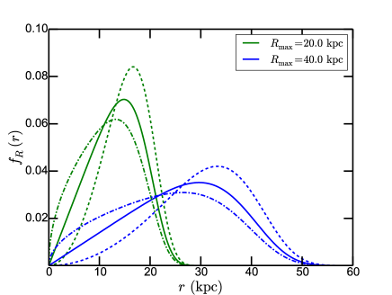
Figure 4: Assumed distribution function of $r$ as described by Eq. (7) for $\eta=0.5$ (dashed-dot lines), $\eta=1$ (solid lines) and $\eta=2$ (dashed lines). The green and the blue curves are for $R_{\rm max}=20$ and 40 kpc, respectively.

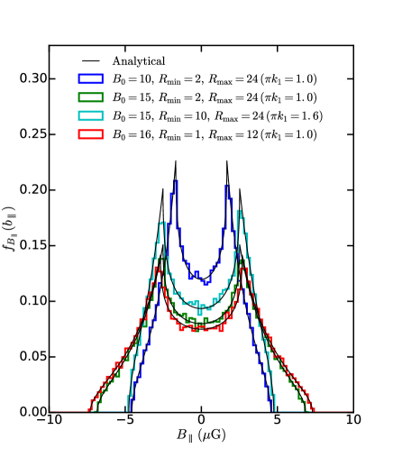
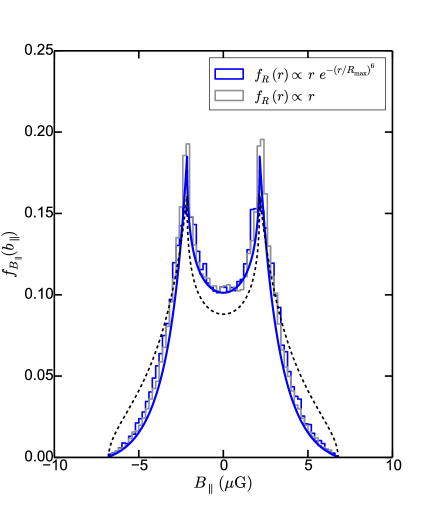
Figure 5: Left: Distribution of $B_{\|}$ for a galaxy inclined at $i=30^{\circ}$ and uniform distribution of radius (Case 2). The black curves are the analytical PDF of a galaxy in Eq. (9). Right: Distribution of $B_{\|}$ for the case when radii are distributed as per Eq. (7) with $\eta=1$ (Case 1) is shown as the blue histogram. The parameters are listed in Table 2. The blue curve is the approximated analytical PDF given in Eq. (11) (see text for details). For comparison, the analytical distribution of $B_{\|}$ for uniform distribution of radii with the same parameters is shown as the dashed line. The grey histogram is the distribution of $B_{\|}$ for the case when the distribution of impact radii given by Eq. (7) is approximated as Eq. (12).

4 Results

4.1 PDF of $B_{\parallel}$ and RM for a single galaxy

We first consider the case of a single galaxy with inclination angle $i$, assuming Case 2 above for the distribution of the radii of the intersecting lines of sight. Applying standard laws pertaining to the distribution functions of random variables (e.g. Sveshnikov, 1968) and to the product of two continuous random functions (e.g. Rohatgi, 1976; Glen et al., 2004) to Eq. (3) (also given by Eq. (24) under our assumptions), we obtain the PDF of $B_{\parallel}$ ($f_{B_{\parallel}}(b_{\parallel})$) for this situation (see Appendix A) as,

$$f_{B_{\parallel}}(b_{\parallel})=\begin{cases}~{}\dfrac{k_{1}}{|b_{\parallel}|}\left[\arcsin\left(\dfrac{|b_{\parallel}|}{a}\right)-\arcsin\left(\dfrac{|b_{\parallel}|}{b}\right)\right],&-a\leq b_{\parallel}\leq a,\\ ~{}\dfrac{k_{1}}{|b_{\parallel}|}\arccos\left(\dfrac{|b_{\parallel}|}{b}\right),&b_{\parallel}\in[-b,-a)\cup(a,b].\\ \end{cases}$$ (9)

Here, $k_{1}=r_{B}/[\pi(R_{\rm max}-R_{\rm min})]$, $a=B_{0}\sin i\,{\rm e}^{-R_{\rm max}/r_{B}}$ and $b=B_{0}\sin i\,{\rm e}^{-R_{\rm min}/r_{B}}$. In left panel of Fig. 5, we compare the analytical PDF of $B_{\parallel}$ to that of simulated distributions to verify the results of the calculation. The simulated distributions were carried out for 10,000 lines of sight, each passing through a galaxy with $B_{\|}$ computed from Eq. 24. The random variables $r$ and $\theta$ were drawn from the distributions described in Section 3.3.

It is evident from Fig. 5 that the PDF of $B_{\|}$ for one galaxy has characteristic features that can be directly used to estimate the strength of the large-scale magnetic field, $B_{0}$. The location of the cusp in the PDF at $a$ is the magnitude of the magnetic field vector projected along the line of sight at the outer edge, while the location of the truncation of the PDF, $b$, is the same but for the inner radius of the ionized disc. $(\pi\,k_{1})^{-1}$ represents the number of radial scale lengths of the magnetic field across the ionized disc. For a galaxy with known values of $R_{\rm min}$ and $R_{\rm max}$, the parameters $a$ and $b$ can be used to estimate $B_{0}$ and $r_{B}$. It can be easily shown that,

$$r_{B}=\frac{R_{\rm max}-R_{\rm min}}{\ln(b/a)}.$$ (10)

Having determined $r_{B}$, $B_{0}\,\sin i$ can be directly evaluated.

For the case when the radii of the intersecting lines of sight are distributed as in Case 1, with $\eta=1$, the PDF of $B_{\|}$ can be approximated as:

$$f_{B_{\parallel}}(b_{\parallel})\approx\begin{cases}~{}\dfrac{k_{2}}{|b_{\|}|}\left(\dfrac{R_{\rm max}}{r_{B}}\right)\left[\arcsin\left(\dfrac{|b_{\|}|}{a}\right)-\arcsin\left(\dfrac{|b_{\|}|}{b}\right)\right],&{}\textstyle\\ ~{}~{}~{}~{}~{}~{}~{}~{}~{}~{}~{}~{}~{}~{}~{}~{}~{}~{}~{}~{}~{}~{}~{}~{}~{}~{}~{}~{}~{}~{}~{}~{}~{}~{}~{}~{}~{}-a\leq b_{\|}\leq a,&\\ ~{}\dfrac{k_{2}}{|b_{\|}|}\ln\left(\dfrac{B_{0}\,\sin i}{|b_{\|}|}\right)\left[\arccos\left(\dfrac{|b_{\|}|}{b}\right)\right],&{}\textstyle\\ ~{}~{}~{}~{}~{}~{}~{}~{}~{}~{}~{}~{}~{}~{}~{}~{}~{}~{}~{}~{}~{}~{}~{}~{}~{}~{}~{}~{}~{}\forall\,\,b_{\|}\in[-b,-a)\cup(a,b].&\end{cases}$$ (11)

Here, $k_{2}=r_{B}/(\pi\,R_{\rm max})$. The right panel of Fig. 5 shows the simulated distribution of $B_{\|}$ (again assuming Case 1 for the distribution of impact radii), and compare this to the analytical results. The location of the cusps in Fig. 5 (left panel) are the same as for Case 2. However, the distributions are slightly wider between the cusps due to the exponential turn-over of the radii distribution in Case 1, while the wings of the distribution of $B_{\|}$ are narrower than those for the case when the impact radii are uniformly distributed.

The approximate analytical form of the PDF given by Eq. (11) was derived by ignoring the exponential cut-off and using a radius range of $0\text{--}{\rm R_{max}}$, i.e., a sharp cut-off at $\rm R_{max}$. In this approximation, the distribution of $r$ is,

$$f_{R}(r)=\frac{\eta+1}{R_{\rm max}^{\eta+1}}\,r^{\eta},~{}~{}~{}0<r<R_{\rm max}\;.$$ (12)

For comparison, the simulated distribution of $B_{\|}$ for the above distribution of $r$ is shown as the grey histogram in Fig. 5 (right panel). The grey and blue histograms show fairly good agreement. Further, in Eq. (11), we have neglected the imaginary terms arising while performing the integrals in Eq. (32). These approximations cause the analytical function in Eq. (11) to underestimate the true distribution of $B_{\|}$ by $\lesssim 10$ per cent, which results in a narrowing of the wings of the analytical function by $\lesssim 5$ per cent.

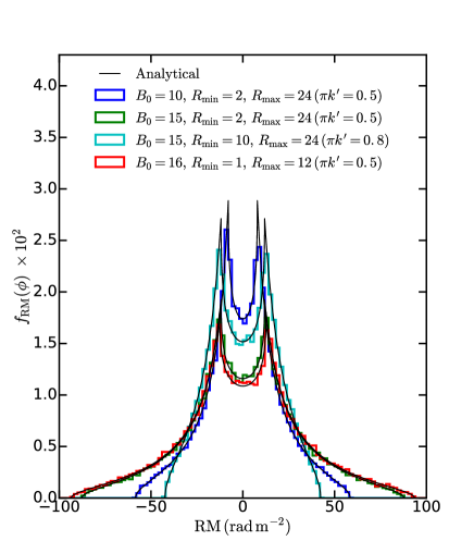
Figure 6: Distribution of RM for a galaxy inclined at $i=30^{\circ}$ for uniform distribution of radius. The black lines are the analytical PDF of RM as given in Eq. (13).

Under our assumptions for the magneto-ionic medium, the RM along each line of sight through a galaxy (given by Eq. (4)) has a form similar to Eq. (24). Therefore, the PDF of RM for Case 2 can be obtained by simply replacing $r_{B}$ by $r_{0}^{\prime}$ and $B_{0}\,\sin i$ by $0.81\,B_{0}\,n_{0}\,h_{\rm ion}\,\tan i$ in Eq. (9). The probability distribution function of RM, $f_{\rm RM}(\phi)$, is then given as,

$$f_{\rm RM}(\phi)=\begin{cases}~{}\dfrac{k^{\prime}}{|\phi|}\left[\arcsin\left(\dfrac{|\phi|}{a^{\prime}}\right)-\arcsin\left(\dfrac{|\phi|}{b^{\prime}}\right)\right],&-a^{\prime}\leq\phi\leq a^{\prime},\\ ~{}\dfrac{k^{\prime}}{|\phi|}\,\arccos\left(\dfrac{|\phi|}{b^{\prime}}\right),&\phi\in[-b^{\prime},-a^{\prime})\cup(a^{\prime},b^{\prime}].\\ \end{cases}$$ (13)

Here, $k^{\prime}=r^{\prime}_{0}/[\pi(R_{\rm max}-R_{\rm min})]$. The parameters $a^{\prime}$ and $b^{\prime}$ are given as,

$$\begin{split}a^{\prime}&=0.81\,B_{0}\,n_{0}\,h_{\rm ion}\tan i\,{\rm e}^{-R_{\rm max}/r^{\prime}_{0}}\\ b^{\prime}&=0.81\,B_{0}\,n_{0}\,h_{\rm ion}\tan i\,{\rm e}^{-R_{\rm min}/r^{\prime}_{0}}.\end{split}$$ (14)

The RM distribution for one galaxy inclined at $i=30^{\circ}$ with different values for the fixed parameters is shown in Fig. 6.

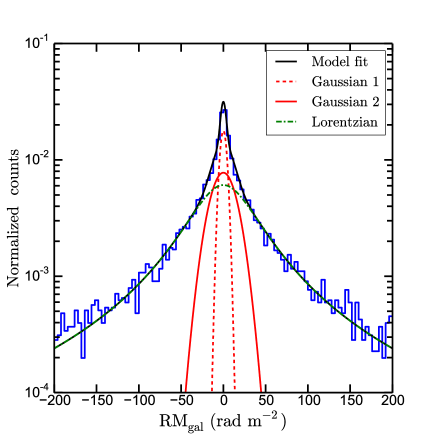
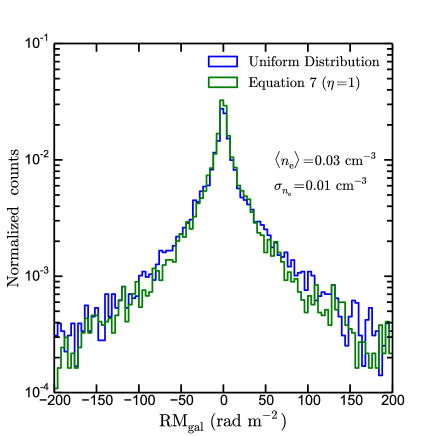
Figure 7: Left: Distribution of ${\rm RM_{gal}}$ for a sample of 10,000 galaxies with uniform distribution of $i$, $\theta$ and $r$ as described in Section 3.3 and, $B_{0}$ and $n_{0}$ of the sample have Gaussian distributions. The parameters used are listed in Table 2. The distribution is modelled as a sum of one Lorentzian and two Gaussian components and is shown as the black solid line. The individual components are shown as green dot-dashed, red solid and dashed lines. Right: Comparison of distribution of ${\rm RM_{gal}}$ when the radius at which the lines of sight intersect the galaxies are distributed uniformly same as left-hand panel (blue histogram) and for the case when they are distributed as in Eq. (7) with $\eta=1$ (green histogram).

The probability distribution of $B_{\parallel}$, and therefore RM, over all azimuthal angles, does not depend on the pitch angle $p$ of the magnetic field. This is because of the $2\pi$-periodicity of $\cos(\theta-p)$. Therefore, it is not possible to determine the pitch angle of the large-scale magnetic field from backlit experiments. However, within a sector of a galaxy, $\theta_{\rm min}\leq\theta\leq\theta_{\rm max}$, where $\theta_{\rm max}-\theta_{\rm min}<\pi$, the function ceases to be periodic. In this case, the PDFs of $B_{\parallel}$ and RM within a segment depend on $p$; this situation is discussed in Appendix A.1.

4.2 The PDF of RM for a sample of galaxies

To simulate a realistic RM distribution for a sample of 10,000 disc galaxies, we computed the RM assuming a single line of sight per galaxy with random distributions of the inclination angle, the azimuthal angle, and the radius of intersection. These parameters have the probability distributions described in Section 3.3. We adopted a normal probability distribution for the strength of the large-scale magnetic field $B_{0}$ of the sample of galaxies, with sample mean $\langle B_{0}\rangle$ and standard deviation $\sigma_{B_{0}}$. Similarly, the free electron density was assumed to have sample mean $\langle n_{\rm e}\rangle$ and standard deviation $\sigma_{n_{\rm e}}$. Thus, the distributions of $B_{0}$ and $n_{\rm e}$ in the sample of galaxies are given as:

$$\begin{split}{\rm PDF}(B_{0})&=\dfrac{1}{\sqrt{2\,\pi\,\sigma_{B_{0}}^{2}}}{\rm exp}\left[\dfrac{-\left(B_{0}-\langle B_{0}\rangle\right)^{2}}{2\sigma_{B_{0}}^{2}}\right]\\ {\rm PDF}(n_{\rm e})&=\dfrac{1}{\sqrt{2\,\pi\,\sigma_{n_{\rm e}}^{2}}}{\rm exp}\left[\dfrac{-\left(n_{\rm e}-\langle n_{\rm e}\rangle\right)^{2}}{2\sigma_{n_{\rm e}}^{2}}\right].\end{split}$$ (15)

The left panel of Fig. 7 shows the simulated distribution of ${\rm RM_{gal}}$ as the blue histogram for the case where the line of sight passes through a sample of absorber systems with a uniform distribution of impact radii (Case 2 of Section 3.3.1). The distinctive features of the RM PDF for a single galaxy described in Section 4.1 are washed out, and we empirically model the PDF of ${\rm RM_{gal}}$ as the sum of one Lorentzian and two Gaussian functions:

$$f_{\rm RM_{gal}}(x)=a_{1}\left[\frac{w_{1}^{2}}{w_{1}^{2}+(x-m_{1})^{2}}\right]+\,a_{2}\,\exp\left[\dfrac{-(x-m_{2})^{2}}{w_{2}}\right]$$

$$+\,a_{3}\,\exp\left[\dfrac{-(x-m_{3})^{2}}{w_{3}}\right].$$ (16)

Here, the parameters $w_{1}$, $w_{2}$ and $w_{3}$ are the characteristic widths of the respective components; $a_{1}$, $a_{2}$ and $a_{3}$ are the amplitude normalizations; and $m_{1}$, $m_{2}$ and $m_{3}$ are the mean values (which are close to zero, as expected). In Eq. (16), $w_{1}$ is in rad m^-2, and $w_{2}$ and $w_{3}$ are in (rad m^-2)². $w_{3}$ is the wider of the two Gaussian components. The fitted PDF is shown as the solid black line in Fig. 7.

The choice of the functions that we used to empirically model the distribution of ${\rm RM_{gal}}$ is motivated by the shape of the PDF of the RM for a single galaxy. The Lorentzian is chosen to capture the wings in the distribution of RM as seen in Fig. 6. Since the cusps at $\pm a^{\prime}$ for one galaxy depend on $B_{0}\,n_{0}$, the distribution should be widened approximately by a Gaussian function if $B_{0}$ and $n_{0}$ have a normal distribution for the galaxy sample. This motivates the choice of the wider of the two Gaussian functions. Finally, the sharp peak at ${\rm RM_{gal}}=0$ rad m^-2 is a manifestation of the distribution of the $\sin i$ function for a uniform distribution of $i$ in the range 0 to $\pi/2$, and the narrower Gaussian accounts for this.

The right panel of Fig. 7 compares the distributions of ${\rm RM_{gal}}$ in Case 2 and Case 1 (where we again assume $\eta=1$ for the radius distribution of the sightlines; see Section 3.3.1), keeping all the other variables the same as in the left panel. The two distributions have negligible overall differences, except that the width of the distribution for Case 1 is marginally smaller than that for Case 2. This does not significantly affect the result of the fit using Eq. (16): the fitted parameters $w_{2}$ and $w_{3}$ are consistent within the errors, with $w_{1}\approx 20$ per cent lower for Case 1 than in Case 2. This is also true for other choices of $\eta$, e.g. $\eta=0.5$ or $\eta=2$. We therefore use Case 2 for the radius distribution of the sightlines in the rest of the paper.

4.3 Model PDF and physical parameters

For a single galaxy, the width of the PDF of ${\rm RM_{gal}}$ depends on two parameters $a^{\prime}$ and $b^{\prime}$, both of which directly depend on $B_{0}$ (see Eq. (14)). We therefore expect the width of the Lorentzian component of the PDF of ${\rm RM_{gal}}$ for a sample of galaxies to depend on $\langle B_{0}\rangle$. In the left-hand panel of Fig. 8, we show the variation of the widths of the different fitted components as a function of $\langle B_{0}\rangle$, for values of $\sigma_{B_{0}}$ in the range $1-10\mu$G. We find that $w_{2}$ varies only weakly with $\langle B_{0}\rangle$, consistent with being constant and with values of $15-20$. However, both $w_{1}$ and $w_{3}$ shows significant variation with $\langle B_{0}\rangle$, with $w_{1}$ showing the strongest dependence on $\langle B_{0}\rangle$ (after taking the errors into account). It should be noted that $\langle B_{0}\rangle$ scales with $\langle n_{\rm e}\rangle$ and $h_{\rm ion}$ as,

$$\left(\dfrac{\langle B_{0}\rangle}{\rm\mu G}\right)\equiv\langle B_{0}\rangle\left(\dfrac{\langle n_{\rm e}\rangle}{\rm 0.03\,cm^{-3}}\right)\left(\dfrac{h_{\rm ion}}{\rm 500\,pc}\right)$$ (17)

It is apparent from Fig. 8 (left-hand panel) that for all values of $\sigma_{B_{0}}$, $w_{1}(\langle B_{0}\rangle)$ converges asymptotically when $\langle B_{0}\rangle\gtrsim\sigma_{B_{0}}$. We empirically model the asymptotic dependence of $w_{1}$ (in $\rm rad\,m^{-2}$) on $\langle B_{0}\rangle$ (in $\mu$G) as,

$$w_{1}(\langle B_{0}\rangle)=p_{0}+p_{1}\,\langle B_{0}\rangle+p_{2}\,\langle B_{0}\rangle^{2}.$$ (18)

The best-fit values of the parameters $p_{0}$, $p_{1}$ and $p_{2}$ are found to be 13.6, 1.8 and $-0.0076$, respectively. The best fit is shown as the dashed line in Fig. 8 (left). Note that we have fixed $w_{2}=18$ (due to its weak dependence on $\langle B_{0}\rangle$) when determining the above empirical dependence $w_{1}(\langle B_{0}\rangle)$. The error due to this assumption on $w_{1}(\langle B_{0}\rangle)$ is $\lesssim 5$ per cent (compared to the case when $w_{2}$ is left as a free parameter). The net error on the estimated $\langle B_{0}\rangle$ is also $\lesssim 5$ per cent.

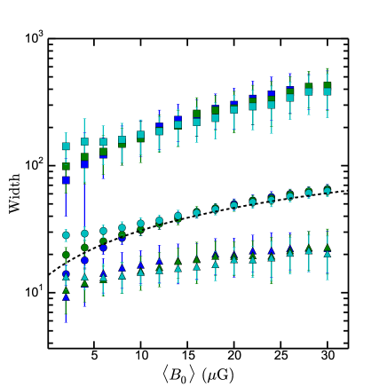
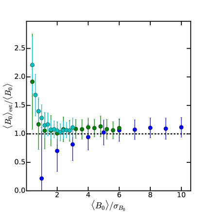
Figure 8: Left: Variation of the widths of the modelled components with $\langle B_{0}\rangle$. Circles, triangles and squares are for $w_{1}$, $w_{2}$ and $w_{3}$, the widths of the Lorentzian and the two Gaussian components, respectively. $w_{1}$ is in rad m^-2 and, $w_{2}$ and $w_{3}$ are in (rad m^-2)². The different colours are for different values of $\sigma_{B_{0}}$ (blue=$2\,\mu$G, green=$5\,\mu$G, cyan=$10\,\mu$G). The dashed line is the empirical fit to $w_{1}$ as a function of $\langle B_{0}\rangle$ given by Eq. (18). Right: Variation of $\langle B_{0}\rangle_{\rm est}/\langle B_{0}\rangle$ as a function of $\langle B_{0}\rangle/\sigma_{B_{0}}$. Here, $\langle B_{0}\rangle_{\rm est}$ is the estimated $\langle B_{0}\rangle$ using Eq. (18). The dashed line is for $\langle B_{0}\rangle_{\rm est}/\langle B_{0}\rangle=1$. The different colours have the same meaning as in the left-hand panel.

When $\langle B_{0}\rangle\lesssim\sigma_{B_{0}}$, $w_{1}$ changes marginally or remains roughly constant at a value that depends on $\sigma_{B_{0}}$. In the right-hand panel of Fig. 8, we show the variation of the ratio of $\langle B_{0}\rangle$ estimated using Eq. (18), $\langle B_{0}\rangle_{\rm est}$, to that of the true $\langle B_{0}\rangle$ in our simulations as a function of $\langle B_{0}\rangle/\sigma_{B_{0}}$. For $\langle B_{0}\rangle/\sigma_{B_{0}}\gtrsim 1$, $\langle B_{0}\rangle_{\rm est}$ agrees well with the true $\langle B_{0}\rangle$, except for the blue points for which $\sigma_{B_{0}}=2\,\mu$G. This is because the parameters $p_{0}$, $p_{1}$ and $p_{2}$ in Eq. (18) are estimated in the regime where $w_{1}$ converges asymptotically in Fig. 8 (left), i.e., for $\langle B_{0}\rangle>10\,\mu$G. This causes $\langle B_{0}\rangle_{\rm est}$ to deviate significantly from $\langle B_{0}\rangle$ for the case where $\sigma_{B_{0}}=2\,\mu$G up to $\langle B_{0}\rangle/\sigma_{B_{0}}\approx 4$. However, we believe that it is unlikely that a sample of galaxies would have $\sigma_{\rm B_{0}}=2\,\mu$G (e.g., Fletcher, 2010), and have hence not extended the fit to account for the above deviation. Thus, in the case where the dispersion of the magnetic field strengths of the galaxies in the sample is larger than their mean field strength, determining $\langle B_{0}\rangle$ will be difficult. This demonstrates the importance of careful selection of the absorber sample: a large variation of galaxy types in the sample is likely to lead to a large $\sigma_{B_{0}}$, which would make it difficult to interpret the results.

Some previous works on this topic, using strong Mgii absorbers as the intervening galaxies, attributed the dispersion in the distribution of RM to predominantly arise from turbulent magnetic fields, typically with RM dispersion $\approx 150~{}\rm rad~{}m^{-2}$ (see, e.g., Bernet et al., 2008; Bernet et al., 2013). It is interesting to note from Fig. 8 (left-hand panel), for a sample of galaxies, the mean large-scale field strength, $\langle B_{0}\rangle$, and its dispersion within the sample, $\sigma_{B_{0}}$, could also give rise to a significant spread in the RM distribution, of a magnitude comparable to that found in the previous studies. Also, the PDF of RM in the presence of large-scale magnetic fields in galaxies deviates from that of a Gaussian. Large sample size in future backlit-experiments could be used to study this deviation from Gaussianity and distinguish between dominating large-scale fields or dominating turbulent fields.

We note that the empirical model given in Eq. (18) does depend on the assumed values for the fixed parameters. In Appendix B, we discuss in detail how different choices of the fixed variables $r_{B}$, $r_{\rm e}$, $R_{\rm min}$, and $R_{\rm max}$, and the assumed distribution of impact radii, i.e., Cases 1 and 2, affect the empirical form of Eq. (18), and hence inferring $\langle B_{0}\rangle$. In the absence of additional constraints on the above free parameters, and considering the typical ranges of values of these parameters, the true value of $\langle B_{0}\rangle$ lies within $\approx 50$ per cent of the value of $\langle B_{0}\rangle$ estimated using Eq. (18).

5 Sample selection criteria for observations

In the light of our results on the statistical properties of the Faraday rotation measure for absorption-selected galaxies, we discuss in this section the selection criteria of the control and the target samples that are important for a better estimation of the large-scale magnetic field properties in the intervening galaxies.

5.1 Redshift coverage of the quasars

As has been pointed out in Section 2.2, differences in the redshift distribution of the background quasars in the target and the control samples can lead to biases when inferring magnetic fields in the intervening galaxies. In fact, there are clear differences in the redshift distributions of the target and control samples that have been used in earlier studies in the literature (e.g. Farnes et al., 2014; Kim et al., 2016). The undesirable bias introduced due to the mismatch in quasar redshifts can be avoided by ensuring the same redshift distribution for the quasars in the target and control samples.

Further, a random selection of quasars from the currently available optical catalogs (e.g. as shown in Fig. 2) will introduce artefacts in the observed PDFs, making it difficult to separate the PDF of the RM contributed by the intervening galaxies from that of the quasars. It is therefore desirable to use a sample that is distributed uniformly in redshift, i.e., with roughly equal number of sources per redshift bin. This would allow the contribution of the $(1+z)^{-2}$ factors to be analytically filtered out.

5.2 The background quasars

Relating the observed PDF of RM to parameters describing the large-scale magnetic field can be greatly simplified if the RM produced by the large-scale fields is unaffected by the RM contributed by turbulent fields in the intervening galaxies and the background polarized quasar remain unresolved within the telescope beam. The former can be achieved when the projected linear extent of the polarized emission from the background quasar encompass several turbulent cells, with the RM contributed by the large-scale field not varying significantly ($\lesssim 10$ per cent) within the illumination beam.

The typical sizes of turbulent cells in nearby galaxies are $\approx 50\text{--}100$ pc (e.g. Ohno & Shibata, 1993; Lazarian & Pogosyan, 2000; Beck, 2016). For intervening galaxies at $z\gtrsim 1$, the angular diameter distance to the foreground absorber and the background quasar is approximately the same. Assuming that the turbulent cell sizes in high-$z$ galaxies are similar to that of the nearby galaxies, we thus require that the spatial extent of the polarized emission in quasars should be $\approx 100\text{--}250$ pc (see Section 5.2.1), i.e. $\approx 25\text{--}50$ mas for quasars at $z\gtrsim 1$. The flat- or inverted-spectrum cores of radio quasars or BL Lac objects are known to emit polarized synchrotron radiation on such scales (e.g. Bondi et al., 1996; Zensus, 1997; Aller et al., 1999; Lister, 2001; Bondi et al., 2004; Lister et al., 2016), and would make good targets for such an RM study. Steep-spectrum polarized sources, e.g. the lobes of radio galaxies, that remain unresolved with the currently available radio telescopes, should be avoided as targets as the projected extended nature of the emission implies that variations in the RM from the large-scale field across the emission region are likely to be significant. Medium-resolution interferometers such as the SKA-MID would also be interesting for such studies, to obtain a synthesized beam of $\approx 50\text{--}100$ mas at GHz-frequencies, which would allow one to resolve out any extended radio emission and study the RM towards the radio core.

5.2.1 Contribution of turbulent fields to ${\rm RM_{gal}}$

We argued qualitatively above that the RM contributed by turbulent fields along each sightline, with rms $b_{\|}$, will be negligible compared to that produced by large-scale fields, $B_{\|}$, for illumination beams of size $\approx 100\text{--}250$ pc at the absorber redshift. Here, we derive this size quantitatively.

The RM produced by $b_{\|}$ over a three-dimensional volume probed by each line of sight has zero mean, and a dispersion ($\sigma_{\rm RM,3D}$) given by

$$\sigma_{\rm RM,3D}=0.81\,\langle n_{\rm e}\rangle\,b_{\|}\,\sqrt{l_{0}\,L}~{}{\rm rad\,m^{-2}}.$$ (19)

Here, $l_{0}$ is the size of the turbulent cells in parsecs, i.e., the correlation scale of the product $n_{\rm e}\,b_{\|}$, while $L=h_{\rm ion}/\cos\,i$ is the path length through the ionized medium. The dispersion of RM in the plane of the sky ($\sigma_{\rm RM,2D}$), averaged over a beam of spatial size $W$ (in pc), is given by $\sigma_{\rm RM,2D}\approx\sigma_{\rm RM,3D}/\sqrt{N}$ (e.g. Fletcher et al., 2011), where $N\approx(W/l_{0})^{2}$ is the number of turbulent cells within the beam area. The effect of turbulent fields is negligible when $\sigma_{\rm RM,2D}/|{\rm RM_{gal}}|\ll 1$. To satisfy this condition, by combining Eqs. (4) and (19), we have

$$W\gg\dfrac{b_{\|}}{|\langle B_{\|}\rangle|}\,l_{0}\,\sqrt{\dfrac{l_{0}\,\cos i}{h_{\rm ion}}}.$$ (20)

For a sample of disc galaxies with uniform distribution of inclination angles, $i$ between 0 and $\pi/2$, the mean value of $\sqrt{\cos i}$ is,

$$\begin{split}\langle\sqrt{\cos i}\rangle&=\dfrac{2}{\pi}\int_{0}^{\pi/2}\sqrt{\cos i}\,\mathrm{d}i\\ &=\left(\dfrac{2}{\pi}\right)^{3/2}\Gamma^{2}\left(\dfrac{3}{4}\right)\approx 0.76\\ \end{split}$$ (21)

For typical parameter values, $b_{\|}/|\langle B_{\|}\rangle|\simeq 2$, $l_{0}\approx 50\text{--}100$ pc and $h_{\rm ion}\approx 500$ pc, we find $W\gg 25\text{--}50$ pc. An illumination beam of size $\approx 100\text{--}250$ pc clearly satisfies this condition. For a larger illumination beam, the variation of the large-scale field within the beam will give rise to $>10$ per cent variation of RM. Hence, to avoid significant contamination from RM arising from the turbulent fields, the background quasars should have polarized emission with a spatial extent of $\approx 100\text{--}250$ pc.

5.3 Intervening objects

Lastly, as noted in Section 4.3, the intervening galaxy sample needs to be carefully chosen so that one does not obtain a large $\sigma_{B_{0}}$ from different populations of galaxies in the sample (as seen in Local Volume galaxies). In order to probe magnetic field evolution in the framework of dynamo action, it is best to use sightlines passing through the discs of galaxies. It is still not clear what galaxy type or ISM conditions are probed by the various absorption lines. In the CGM, mostly probed by systems that show Civ absorption and/or Lyman-limit systems (LLSs), the magnetic field could be of non-dynamo origin, e.g., the primordial seed field amplified by magneto-rotational instability (MRI), tidal interactions, and/or gas inflow or outflow.

In the local Universe, Hi column densities within the $R_{25}$ radius have values $N_{\rm HI}\gtrsim 2\times 10^{20}$ cm^-2. This threshold value for $N_{\rm HI}$ is hence a good indicator whether the absorbing gas lies within a galaxy (e.g. Wolfe et al., 2005). However, the galaxy type, and even whether the absorber is a disc galaxy or a dwarf, cannot be directly inferred from the Hi column density. Additional information on the gas phase metallicities ([M/H]; e.g. Pettini et al. 1994; Rafelski et al. 2012), kinematics, and/or gas temperatures is essential to glean information on the nature of the absorber host. Here, we discuss briefly the properties of two main absorber classes that are used as tracers of galaxies at high redshifts, namely, Mgii absorbers and DLAs.

Intervening Mgii absorbers: Strong Mgii$\lambda 2796\AA$ absorbers at intermediate redshifts have long been associated with the presence of galaxies close to the quasar sightline (e.g. Bergeron & Boissé, 1991). Today, more than 40,000 strong Mgii$\lambda 2796\AA$ absorbers are known, mostly at $0.4<z<2.3$, from studies based on the SDSS (e.g. Nestor et al., 2005; Zhu & Ménard, 2013). Follow-up Lyman-$\alpha$ absorption studies of Mgii absorbers have shown that damped Lyman-$\alpha$ absorption (which is expected to arise from sightlines intersecting galaxy discs) is only seen for Mgii$\lambda 2796\AA$ rest equivalent widths $W_{0}^{\lambda 2796}\gtrsim 0.5$ Å (Rao et al., 2006). Intermediate-strength Mgii absorbers (with $W_{0}^{\lambda 2796}\approx 0.3\text{--}0.5$ Å) are expected to trace the outskirts of galaxies or high velocity clouds (Nestor et al., 2005; Nestor et al., 2007). It should be emphasized, however, that a high rest equivalent width $W_{0}^{\lambda 2796}>0.5$ Å does not guarantee the presence of damped Lyman-$\alpha$ absorption. Rao et al. (2006) found that only $\approx 35$ per cent of Mgii absorbers with $W_{0}^{\lambda 2796}>0.5$ Å have $N_{\rm HI}\geq 2\times 10^{20}$ cm^-2. Two-thirds of strong Mgii absorber sightlines thus appear to trace clouds in the circumgalactic medium, galactic superwinds, etc., rather than galaxy discs (e.g. Bond et al., 2001; Zibetti et al., 2007; Neeleman et al., 2016). The magnetic fields in these regions could be of completely different origin from those in the discs, and, at least as important, is likely to have diverse origins as mentioned above. A target sample of galaxies chosen only by the presence of strong Mgii absorption is thus unlikely to be suitable as a probe of dynamo action in high-$z$ galaxies. We note that most backlit-experiment studies of magnetic fields in high-$z$ galaxies have so far been based on such strong Mgii absorbers (e.g. Bernet et al., 2008; Bernet et al., 2013; Joshi & Chand, 2013; Farnes et al., 2014; Kim et al., 2016). But, they don’t necessarily treat them as dynamo origin.

Intervening damped Lyman-$\alpha$ absorbers: DLAs have the highest Hi column densities of all absorbers, $N_{\rm HI}\geq 2\times 10^{20}$ cm^-2 (Wolfe et al., 2005), column densities that only arise in galaxies in the local Universe. The presence of damped Lyman-$\alpha$ absorption in a quasar spectrum has hence long been used to infer the presence of a galaxy along the quasar sightline (Wolfe et al., 1986). Unfortunately, such high Hi column densities can arise in a wide range of galaxy types, ranging from massive disc galaxies through small dwarfs. Additional selection criteria must hence be imposed on DLA samples to reduce the heterogeneity of the underlying population.

Unfortunately, the presence of the bright quasar close to the DLA host galaxy has meant that it has been very difficult to use optical imaging studies to characterize the nature of DLA host galaxies. Only around a dozen DLAs at $z\gtrsim 2$ have identified host galaxies (e.g. Krogager et al., 2012), and even this small sample is heavily biased towards high-metallicity absorbers. Recently, imaging of a sample of foreground DLAs at wavelengths shortward of the Lyman break produced by higher-redshift absorbers on the same sightline has shown that DLAs at $z\approx 2.7$ appear to typically have very low star formation rates, $\lesssim 0.5\,\rm M_{\odot}\,yr^{-1}$ (Fumagalli et al., 2014, 2015). This suggests that the DLA host galaxy population at $z\gtrsim 2$ may be dominated by dwarf galaxies. Unfortunately, dwarf galaxies can only host weak mean-field dynamos and hence should be separated from the target sample when studying the evolution of the large-scale magnetic fields in disc galaxies.

One hence needs a spectroscopic indicator of the nature of the host galaxy, that might allow us to select disc galaxies out of the general DLA population. There are two obvious possibilities: (1) the Hi spin temperature, and (2) the gas-phase metallicity.

The Hi spin temperature ($T_{\rm s}$) provides insights on the temperature distribution of neutral gas in the ISM (Heiles & Troland, 2003; Roy et al., 2013; Chengalur & Kanekar, 2000). This allows one to statistically distinguish between large disc galaxies (which contain significant amounts of cold gas, and hence have a low $T_{\rm s}$) and dwarf galaxies (where the gas is mostly warm, and which hence have a high $T_{\rm s}$). In order to infer $T_{\rm s}$, it is necessary to carry out redshifted Hi 21-cm absorption studies of all the target absorption-selected galaxies. A combination of poor low-frequency frequency coverage and radio frequency interference have meant that there are only $\approx 50$ DLAs in the literature with searches for redshifted Hi 21-cm absorption (e.g. Wolfe & Davis, 1979; Wolfe et al., 1985; Kanekar et al., 2006; Kanekar et al., 2007, 2014).

While Hi 21-cm absorption studies of large DLA samples are likely to be possible in the future with new low-frequency telescopes (e.g. Kanekar, 2014), especially towards the target absorbers of our proposed RM studies (due to the compactness of radio structure of the background quasars), we suggest that the more easily-measured gas-phase metallicity would be a better tool to distinguish between disc and dwarfs galaxies. Metallicity estimates are now available for more than 300 DLAs at a wide range of redshifts, using tracers that are relatively insensitive to dust depletion (e.g. Pettini et al., 1994, 1997, 1999; Prochaska et al., 2003, 2007; Kulkarni et al., 2005; Akerman et al., 2005; Rafelski et al., 2012). Evidence has been found for a mass-metallicity relation in DLAs (e.g. Møller et al., 2013; Neeleman et al., 2013), similar to that in emission-selected galaxies (e.g. Erb et al., 2006), indicating that high-metallicity absorbers are statistically likely to trace the more-massive disc galaxies.

High-metallicity DLAs at high redshifts have been found to show higher star formation rates than the typical DLA population (e.g. Fynbo et al., 2011, 2013; Krogager et al., 2013). Hi 21-cm absorption studies of DLA samples have shown that the gas phase metallicity is anti-correlated with the spin temperature, with high-metallicity DLAs having lower spin temperatures (Kanekar & Chengalur, 2001; Kanekar et al., 2009). Recently, Neeleman et al. (2017) obtained the first detection of [Cii] 158-$\mu$m emission in high-metallicity DLAs at $z\approx 4$, confirming that the absorbers are massive star-forming galaxies with rotating discs. Thus, choosing target DLAs based on a high metallicity ([M/H] $\gtrsim-0.5$; e.g. Rafelski et al. 2012), appears to be the best way to target disc galaxies at $z\gtrsim 2$. One might also use comparisons of RM between DLA samples at different mean metallicities (e.g. [M/H] $\approx-0.5$, $\approx-1.5$ and $\approx-2.5$) to study the cosmic evolution of magnetic fields in very different galaxy environments. This could help to assess the importance and efficacy of dynamo action as a function of galaxy mass.

Further, we note that it is straightforward to detect the presence of a DLA along a quasar sightline with even low-resolution spectroscopy, with $R\lesssim 2000$. However, measuring DLA metallicities usually requires follow-up spectroscopy with both high resolution ($R\gtrsim 10,000$) and high sensitivity. This may prove difficult for very large target galaxy samples. However, a relatively tight correlation has been detected between the rest equivalent width of the Siii$\lambda$1526Å line and the DLA metallicity, and it should be possible to detect this Siii transition in high-metallicity DLAs via low-resolution spectroscopy (Prochaska et al., 2008). One might hence instead use the threshold $W_{0}^{\lambda 1526}\gtrsim 2$Å based on the detection spectra to identify high-metallicity DLAs in the sample.

6 Future work

Our calculations and results are based on the assumption that magnetic fields in galaxies are confined to the disc with axisymmetric large-scale field. This assumption is unlikely to be strictly correct. A detailed treatment of the full three-dimensional magnetic field structure including the vertical magnetic field, e.g. dipolar or quadrupolar configurations (Ruzmaikin et al., 1988; Sokoloff & Shukurov, 1990; Beck et al., 1996), will be considered in a forthcoming paper.

In addition to the dynamo-generated vertical magnetic fields, the effects of galactic outflows due to star formation activity also should be considered. Star formation drives magnetized outflows on galactic scales (Chyży et al., 2016; Damas-Segovia et al., 2016; Wiener et al., 2017) which can affect the form of our derived PDF of RM and thereby affect the interpretations. A careful treatment of the magnetized outflow is necessary in order to study galactic magnetic fields during the peak epoch of cosmic star formation history.

The effects of the RM contributed by turbulent magnetic fields can be minimized by choosing background quasars such that the three-dimensional volume probed by the illumination beam through the intervening galaxy contains several turbulent cells. This simplifies our calculations of ${\rm RM_{gal}}$ and helps to measure the properties of the large-scale disc field. Turbulent fields are themselves important for a complete understanding of the magneto-ionic medium in galaxies. The energy density in the turbulent fields are significantly larger than that in the large-scale field (Beck et al., 1996; Beck & Wielebinski, 2013; Beck, 2016) and contributes substantially to the pressure balance in the ISM (Beck, 2007; Basu & Roy, 2013; Beck, 2016). Further, the ratio of the strength of the random field to that of the large-scale field can provide additional constraints on the magnetic field geometry (Shukurov, 2007; Mao et al., 2017). The effects of turbulent fields in the intervening galaxies will appear as additional wavelength-dependent depolarization of the linearly polarized signal of the background quasars in the target sample, as compared to quasars in the control sample. This scenario is being investigated in another paper of this series.

The success of these backlit-experiments depends crucially on how well one can model the contribution of ${\rm RM_{c}}$, and how accurately it can be isolated in the observed distribution of ${\rm RM_{t}}$ to obtain the distribution of ${\rm RM_{gal}}$. In order to achieve the best results we suggest the following modification to Eq. (1):

$$\begin{split}{\rm RM_{t}^{\prime}}&=(1+{z_{\rm gal}})^{2}\,{\rm RM_{t}}\\ &={\rm RM_{gal}}+{(1+{z_{\rm gal}})^{2}}\,{\rm RM_{qso}^{\prime}}.\end{split}$$ (22)

This approach would minimize the redshift dilution of ${\rm RM_{gal}}$. Similarly, one could modify ${\rm RM_{c}}$ to:

$${\rm RM_{c}^{\prime}}=(1+z_{\rm r})^{2}\,{\rm RM_{c}}.$$ (23)

Here, $z_{\rm r}$ are values randomly drawn from the set of the sample values of ${z_{\rm gal}}$. This operation is possible for a large enough sample and it can be shown that ${\rm PDF}[{(1+{z_{\rm gal}})^{2}}\,{\rm RM_{qso}^{\prime}}]={\rm PDF}[(1+z_{\rm r})^{2}\,{\rm RM_{c}}]$. However, the number of sightlines required depends on the decomposition of PDFs (see Eq. (22)). We are investigating the points raised in this section in a series of forthcoming papers.

7 Summary

To infer the properties of large-scale magnetic fields in high-$z$ disc galaxies through backlit-experiments, we have derived analytical expressions for the probability distributions of $B_{\|}$ and RM for a galaxy with an axisymmetric spiral field geometry. We extend this to a sample of disc galaxies and present an empirical model of the RM distribution when random lines of sight are shot through galaxies with a random distribution of inclination angles, impact radii, strengths of the large-scale magnetic field, and free electron densities. Our study is applicable to future backlit-experiments where the RM produced in the galaxies has been isolated from other RM contributions along the line of sight, i.e., RM arising from the background quasar, the IGM and the Milky Way. The main findings of this study are:

1. We demonstrate that the methods used in the literature to statistically infer the large-scale magnetic field strength in samples of high-redshift galaxies are likely to suffer from significant biases. The biases arise from using the absolute value of RMs, the different redshift coverages of background quasars in the target and control samples, and incomplete redshift coverage of absorber systems in the currently available data.

2. Under our assumed model of the magneto-ionic medium for a galaxy, the distributions of $B_{\|}$ and RM for a single galaxy observed along randomly chosen lines of sight have distinctive features that are dependent on the strength and radial scale-length of the large-scale magnetic field, and the radius range probed by the sight lines.

3. The distributions of $B_{\|}$ and RM are independent of the pitch angle of the magnetic field when the lines of sight through a galaxy sample all azimuthal angles. However, within segments of azimuthal angles, the distributions depend on the magnetic pitch angle.

4. The dispersion in the Faraday rotation arising only from large-scale magnetic fields in intervening galaxies can give rise to a significant spread in the distribution of the RM for a galaxy sample, of a magnitude comparable to that found in previous studies.

5. For a sample of galaxies, where each galaxy has random $i$, $B_{0}$, $n_{0}$ and the lines of sight probe random distances from the centre, the distribution of RM can be empirically modelled as a sum of one Lorentzian and two Gaussian functions.

6. The width of the Lorentzian function ($w_{1}$) gives an estimate of the mean magnetic field strength, $\langle B_{0}\rangle$, of the sample, provided the sample dispersion, $\sigma_{B_{0}}$, is sufficiently small, i.e., $\langle B_{0}\rangle/\sigma_{B_{0}}\gtrsim 1$. This emphasizes the importance of selecting absorber galaxies carefully so as to avoid heterogeneous galaxy samples.

7. Choosing disc galaxies as a target sample is critical to study the evolution of large-scale magnetic fields in the future work on disc dynamo action. This selection criterion is best achieved when the galaxies are identified as damped Lyman-$\alpha$ absorbers with high metallicities. Comparing Faraday rotation in spiral and dwarf galaxies (the latter are not expected to host mean-field dynamos) can shed light on conditions for, and the consequences, of galactic dynamo action.

Appendix A Probability distribution functions

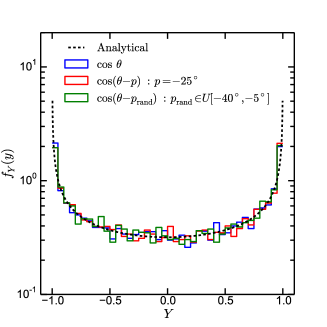
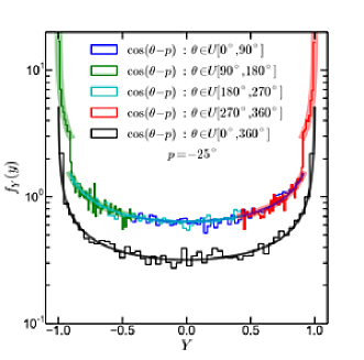
Figure 9: Left: Distribution of $\cos\theta$ (blue histogram), $\cos(\theta-p)$ with constant $p=-25^{\circ}$ (red histogram) and $\cos(\theta-p_{\rm rand})$ with $p_{\rm rand}$ uniformly distributed, such that, $p_{\rm rand}\in U[-40^{\circ},-5^{\circ}]$ (green histogram). Here, $\theta$ is distributed uniformly between $0^{\circ}$ and $360^{\circ}$. The black dashed curve is the analytical PDF given in Eq. (26). Right: Distribution of $Y=\cos(\theta-p)$ for $p=-25^{\circ}$. Each colour is for for uniform distribution of $\theta$ lying in the range $n\times 90^{\circ}$ and $(n+1)\times 90^{\circ}$, where $n=0,1,2,3$. The corresponding curves are the analytical functions given by Eqns. (28) and (29). For comparison, we show the distribution for $\theta$ in the range $0-360^{\circ}$ in black, same as the left-hand panel.

Under assumptions described in Section 3, the magnetic field along the line of sight ($B_{\rm\parallel}$) in Eq. (3) is given by,

$$B_{\parallel}=-B_{0}\,{\rm e}^{-r/r_{B}}\,\cos(\theta-p)\,\sin\,i.$$ (24)

The probability distribution function, $f_{Y}(y)$, of function of a random variable $X$, where $Y=f(X)$ and $X=f^{-1}(Y)$ is single valued, is given by (Sveshnikov, 1968),

$$f_{Y}(y)=f_{X}[f^{-1}(y)]\left|\frac{df^{-1}(y)}{dy}\right|.$$ (25)

Here, $f^{-1}$ denotes the inverse function.

Thus, we compute the PDF of $Y=\cos(\Theta-p)$, i.e., $f_{Y}(y)$, as:

$$f_{Y}(y)=\begin{cases}~{}\dfrac{1}{\pi\sqrt{1-y^{2}}},&\text{for }-1\leq y\leq 1,\\ ~{}0,&\text{otherwise.}\\ \end{cases}$$ (26)

Interestingly, the PDF of $\cos(\theta-p)$ is independent of the value of the pitch angle $p$ because of the periodicity of the function in $0\leq\theta<2\pi$. In Fig. 9 (left-hand panel), we show the distribution of the functions $\cos(\theta)$ and $\cos(\theta-p)$ with constant $p$ and $\cos(\theta-p_{\rm rand})$ with uniform distribution of $p_{\rm rand}$ from $-40^{\circ}$ to $-5^{\circ}$. Clearly, as the PDF is independent of $p$, all the distributions can be represented by a single analytical form.

However, within segments of a galaxy, i.e.,

$$f_{\Theta}(\theta)=\begin{cases}~{}\dfrac{1}{\theta_{\rm max}-\theta_{\rm min}},&\text{for }\theta_{\rm min}\leq\theta\leq\theta_{\rm max},\\ ~{}0,&\text{otherwise,}\\ \end{cases}$$ (27)

where $\theta_{\rm max}-\theta_{\rm min}<\pi$ and $0,\pi,2\pi\not\in(\theta_{\rm min}-p,\theta_{\rm max}-p)$, the PDF of $\cos(\theta-p)$ is given by

$$f_{Y}(y)=\begin{cases}~{}\left(\dfrac{1}{\theta_{\rm max}-\theta_{\rm min}}\right)\left(\dfrac{1}{\sqrt{1-y^{2}}}\right),&{}\textstyle\\ ~{}~{}~{}~{}~{}~{}~{}~{}~{}~{}~{}y\in\,[\cos(\theta_{\rm min}-p),\,\cos(\theta_{\rm max}-p)],&\\ ~{}0,~{}~{}~{}~{}~{}~{}\text{otherwise.}&{}\textstyle\\ \end{cases}$$ (28)

In the cases where $0,\pi,2\pi\in(\theta_{\rm min}-p,\theta_{\rm max}-p)$, the distribution is given by,

$$f_{Y}(y)=\begin{cases}~{}\left(\dfrac{1}{\theta_{\rm max}-\theta_{\rm min}}\right)\left(\dfrac{1}{\sqrt{1-y^{2}}}\right),&{}\textstyle\\ ~{}~{}~{}~{}~{}~{}~{}~{}~{}~{}~{}~{}~{}~{}y\in\,[\cos(\theta_{\rm min}-p),\,\cos(\theta_{\rm max}-p)],&{}\textstyle\\ ~{}\left(\dfrac{2}{\theta_{\rm max}-\theta_{\rm min}}\right)\left(\dfrac{1}{\sqrt{1-y^{2}}}\right)\,\Pi_{\cos(\theta_{\rm max}-p),(+,-)1}(y),&{}\textstyle\\ ~{}~{}~{}~{}~{}~{}~{}~{}~{}~{}~{}~{}~{}~{}~{}~{}~{}~{}~{}y\in[\cos(\theta_{\rm max}-p),(+,-)1],&{}\textstyle\\ ~{}0,~{}~{}~{}~{}~{}~{}~{}~{}~{}~{}~{}\text{otherwise.}&{}\textstyle\\ \end{cases}$$ (29)

Here, $\Pi_{a,(+,-)1}(y)$ represents the boxcar function in the range $\cos(\theta_{\rm max}-p)$ and $(+,-)1$ if $2\pi,\pi\in(\theta_{\rm min}-p,\theta_{\rm max}-p)$. The distribution of $\cos(\theta-p)$ within segments of $\pi/2$ in azimuthal angles is shown in Fig. 10. Note that the above analytical description is valid for segments of length $\pi/2$ with $\theta_{\rm min}=n\times\pi/2$ and $|p|<\pi/4$. For a general treatment, the segments where $\cos(\theta-p)$ no longer remain single valued need to be considered appropriately.

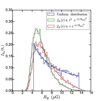
Figure 10: Distribution of the function $B_{R}=B_{0}\,{\rm e}^{-r/r_{B}}$ for a uniform distribution of $r$ given by $U[R_{\rm min},R_{\rm max}]$ (blue histogram) and for the case when $r$ is distributed as per Eq. (7) with $\eta=1$ (red histogram) and $\eta=2$ (green histogram). The corresponding curves are the analytical PDFs given in Eqs. (30) and (31).

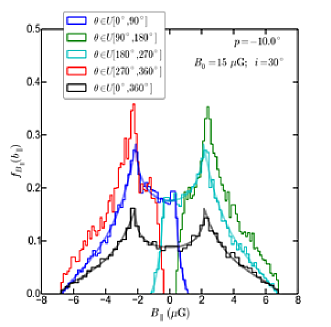
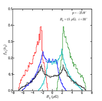
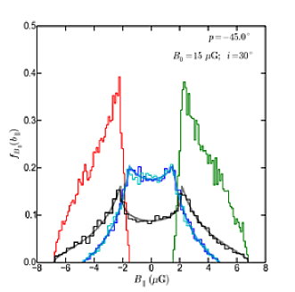
Figure 11: Distribution of $B_{\parallel}$ for a single galaxy which is inclined at $30^{\circ}$ and $B_{0}=15~{}\mu$G. Different colours are for different different segments of azimuthal angle $\theta$. For comparison we also show the PDF of $B_{\parallel}$ for the entire galaxy as the black histogram. The different panels are for different values of the pitch angle $p$. It is evident from the distributions, the PDF of $B_{\parallel}$ is independent of $p$ for the entire galaxy. However, within the different segments, the distribution depends on the pitch angle.

Similarly, the PDF of $B_{R}=B_{0}\,{\rm e}^{-r/r_{B}}$, $f_{B_{R}}(b_{r})$, for a uniform distribution of $r$ (Case 2 in Section 3.3.1) is given by,

$$f_{B_{R}}(b_{r})=\begin{cases}~{}\dfrac{r_{B}}{(R_{\rm max}-R_{\rm min})\,b_{r}},&B_{0}{\rm e}^{-R_{\rm max}/r_{B}}\leq b_{r}\leq B_{0}{\rm e}^{-R_{\rm min}/r_{B}},\\ ~{}0,&\text{otherwise.}\end{cases}$$ (30)

In the case where $r$ is distributed according to Eq. (7) (Case 1 in Section 3.3.1), the PDF of $B_{R}$ has the form,

$$\begin{split}f_{B_{R}}(b_{r})&=\frac{6}{\Gamma\left(\frac{\eta+1}{6}\right)}\,\left(\frac{r_{B}}{R_{\rm max}}\right)^{\eta+1}\,\frac{1}{b_{r}}\,\left[-\ln\left(\frac{b_{r}}{B_{0}}\right)\right]^{\eta}\,{\rm e}^{-\left[\frac{r_{B}}{R_{\rm max}}\,\ln\left(\frac{b_{r}}{B_{0}}\right)\right]^{6}},\\ &~{}~{}~{}~{}~{}~{}~{}~{}~{}~{}~{}~{}~{}~{}~{}~{}~{}~{}~{}~{}~{}~{}~{}~{}~{}~{}~{}~{}~{}~{}~{}~{}~{}~{}~{}~{}~{}~{}~{}~{}~{}~{}0\,\leq\,b_{r}\,\leq\,B_{0}.\end{split}$$ (31)

The distributions of $B_{0}\,{\rm e}^{-r/r_{B}}$ for the above two cases are shown in Fig. 9 (right panel) for $B_{0}=15~{}\mu$G, $r_{B}=20$ kpc, and $R_{\rm min}$ and $R_{\rm max}$ equal to 2 and 25 kpc, respectively.

A.1 Distribution function of $B_{\|}$ and RM for a single galaxy

The probability density of the product of two continuous random variables ($V=XY$) is given by (Rohatgi, 1976; Glen et al., 2004),

$$f_{V}(v)=\int_{-\infty}^{+\infty}f_{X,Y}\left(x,v/x\right)\frac{1}{|x|}dx.$$ (32)

Here, $f_{X,Y}(x,y)$ is the joint PDF of the continuous variables $X$ and $Y$. Applying the above relation to Eq. (24), we compute the PDF of $B_{\parallel}$, $f_{B_{\parallel}}(b_{\parallel})$, for a galaxy as a function of $B_{0}$, $i$ and $r_{B}$ as,

$$f_{B_{\parallel}}(b_{\parallel})=\begin{cases}~{}\dfrac{k_{1}}{|b_{\parallel}|}\left[\arcsin\left(\dfrac{|b_{\parallel}|}{a}\right)-\arcsin\left(\dfrac{|b_{\parallel}|}{b}\right)\right],&-a\leq b_{\parallel}\leq a,\\ ~{}\dfrac{k_{1}}{|b_{\parallel}|}\,\arccos\left(\dfrac{|b_{\parallel}|}{b}\right),&b_{\parallel}\in[-b,-a)\cup(a,b].\\ \end{cases}$$ (33)

Here, $k_{1}=r_{B}/[\pi(R_{\rm max}-R_{\rm min})]$, $a=B_{0}\sin i\,{\rm e}^{-R_{\rm max}/r_{B}}$ and $b=B_{0}\sin i\,{\rm e}^{-R_{\rm min}/r_{B}}$. The distribution of $B_{\parallel}$ is shown in the right panel of Fig. 5.

As discussed above, the distribution function is independent of the pitch angle because of the periodicity of $\cos(\theta-p)$ in the range from $0$ to $2\pi$. However, within segments of azimuthal angles in a galaxy, the symmetry no longer holds true, making the PDF within each segment dependent on the pitch angle. In Fig. 11 we show the segment-wise PDF of $B_{\parallel}$ for various values of $p$. In this case, the locations of the characteristic peaks of the PDF (at $\pm a$) are modified to $a\,\cos(\theta_{\rm min}-p)$ and $a\,\cos(\theta_{\rm max}-p)$ in the segments $[0,90^{\circ}]$ and $[180^{\circ},270^{\circ}]$, respectively.

Since the RM along each line of sight through a galaxy as given by Eq. (4) has the same form as that of Eq. (24), the analytical form of the PDF of RM can be similarly written, replacing $r_{B}$ by $r_{0}^{\prime}$ and $B_{0}\,\sin i$ by $0.81\,B_{0}\,n_{0}\,h_{\rm ion}\,\tan i$.

Appendix B Variation of ${\rm RM_{gal}}$ distribution

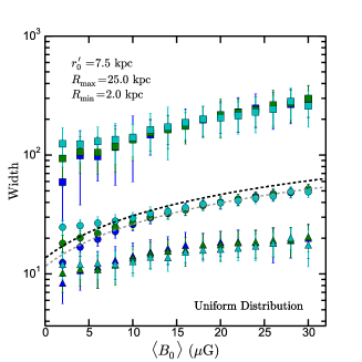
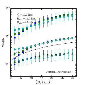
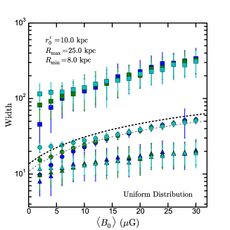
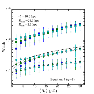
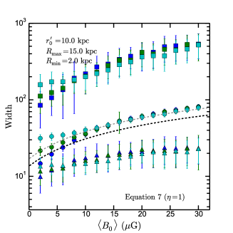
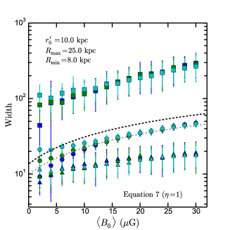
Figure 12: Variation of the widths of the modelled components to fit the PDF of ${\rm RM_{gal}}$ with $\langle B_{0}\rangle$ for radii distribution as per Case 2 (top panels) and Case 1 with $\eta=1$ (bottom panels). The different columns are for different choices of the fixed parameters listed in the top left corner of the plots. The symbols and colours have the same meaning as in Fig. 8. Black dashed curve is the empirical fit given by Eq. (18) and the grey dashed curve is obtained by scaling the black curve with factors listed in Table 1.

Table 1: Scaling factor ($a_{\rm s}$) to be applied to Eq. (18) for different choices of fixed parameters.

Radial distribution	$R_{\rm min}$, $R_{\rm max}$	$r_{0}^{\prime}$	$r_{B}$, $r_{\rm e}$	$a_{\rm s}$
	(kpc)	(kpc)	(kpc)
Uniform	2, 25	12.5	25, 25	1.18
(Case 2)		10	20, 20	1.00
		7.5	15, 15	0.85
		7.5	20, 12	0.85
		5	20, 6.67	0.69
		5	10, 10	0.69
		3.75	15, 5	0.64
	0, 25	10	20, 20	1.12
	2, 35	10	20, 20	0.86
	2, 45	10	20, 20	0.78
	8, 25	10	20, 20	0.78
	2, 15	10	20, 20	1.34
	8, 35	10	20, 20	0.64
	8, 35	7.5	15, 15	0.51
Eq. (7); $\eta=1$	2, 25	10	20, 20	0.80
(Case 1)		7.5	15, 15	0.64
		5	10, 10	0.51
	8, 25	10	20, 20	0.71
	2, 15	10	20, 20	1.21

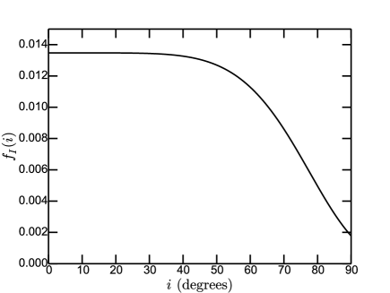
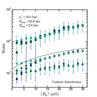
Figure 13: Left: Modified distribution of inclination angle of galaxies given by Eq. (35). Right: Variation of the widths of the components to model the PDF of ${\rm RM_{gal}}$ with $\langle B_{0}\rangle$ for uniform distribution of radii and inclination angles distributed as shown in the left panel. The symbols and colours have the same meaning as in Fig. 8. The black dashed curve is the empirical model given by Eq. (18) and the grey curve is obtained by scaling the black curve by a factor 0.78.

Here, we assess how the empirical modelling describing the variation of $w_{1}$ with $\langle B_{0}\rangle$ in Eq. (18) changes for different assumptions for the fixed parameters, such as the distribution of radii, radial scale-lengths, and inclination angles.

In Fig. 12, we show the variation of $w_{1}$, $w_{2}$ and $w_{3}$ with $\langle B_{0}\rangle$ for different choices of the fixed parameters. For the top panels, the radii of intersection are distributed uniformly, i.e., Case 2 in Section 3.3.1, while, for the bottom panels, the radii are distributed as per Case 1 with $\eta=1$. The different columns are for different choices of the fixed parameters. For all the cases, the PDF of ${\rm RM_{gal}}$ is modelled as a sum of one Lorentzian and two Gaussian functions described in Section 4.2. We find that $w_{1}$ is typically $\sim 20$ per cent lower for Case 1 as compared to Case 2, for the same set of parameters (see the bottom panel of Fig. 12). The black dashed curve is the empirical model given by Eq. (18) and Fig. 8, i.e., for Case 1 only. We find that the overall dependence of $w_{1}$, $w_{2}$ and $w_{3}$ on $\langle B_{0}\rangle$ does not significantly depend on the assumed values of the fixed parameters. The empirical model for the variation of $w_{1}$ with $\langle B_{0}\rangle$ can be made to fit the data by scaling Eq. (18) as,

$$w_{1}\left(\langle B_{0}\rangle\right)=a_{\rm s}\,\left(p_{0}+p_{1}\,\langle B_{0}\rangle+p_{2}\,\langle B_{0}\rangle\right),$$ (34)

where $a_{\rm s}$ is a scaling factor whose values for different choices of the fixed parameters are listed in Table 1. The scaled empirical models are shown as the grey dashed curves in Fig. 12.

B.1 Effect of radial scale length

The location of the cusps and the width of the PDF of ${\rm RM_{gal}}$ for a single galaxy (Eq. (13)) depends on the effective radial scale length, $r_{0}^{\prime}$, of the product $n_{\rm e}\,B_{\|}$ as $\exp(-R_{\rm min}/r_{0}^{\prime})$ and $\exp(-R_{\rm max}/r_{0}^{\prime})$, respectively. Thus, we expect the width of the PDF of ${\rm RM_{gal}}$ for a sample of galaxies to depend on $r_{0}^{\prime}$ such that $w_{1}$ should decrease with decreasing $r_{0}^{\prime}$. Such a behaviour can indeed be seen in both Table 1 and the top-left panel of Fig. 12. In fact, as expected, the overall width of the PDF of ${\rm RM_{gal}}$ does not depend on the individual radial scale lengths of $B_{\|}$ or $n_{\rm e}$, i.e., $r_{B}$ or $r_{\rm e}$, respectively. The scale factor changes by $\lesssim 40$ per cent within the typical range of values of $r_{0}^{\prime}$. This results in $\langle B_{0}\rangle$ being constrained within $\approx 50$ per cent of its true value, while estimating it using the set of fixed parameters in Eq. (18).

B.2 Effect of $R_{\rm min}$ and $R_{\rm max}$

$R_{\rm min}$ and $R_{\rm max}$ will have an opposite effect on the width of the distribution of ${\rm RM_{gal}}$ for a sample of galaxies as compared to $r_{0}^{\prime}$, i.e., we expect the widths to decrease with increasing $R_{\rm min}$ and $R_{\rm max}$. In the middle panels of Fig. 12, we show the variation of the widths of the fitted components with $\langle B_{0}\rangle$ for $R_{\rm max}=15$ kpc. Clearly, the values of $w_{1}$ in this case are larger by a factor of $\approx 1.3$ (see Table 1) than those for the case $R_{\rm max}=25$ kpc, which was used to model Eq. (18).

In the right-hand panels of Fig. 12 show that $w_{1}$ decreases by a factor of $\approx 0.8$ on increasing $R_{\rm min}$ from 2 kpc to 8 kpc. We note that $R_{\rm min}$ is not expected to vary widely for a given absorption line species. For example, for the case of DLAs, $R_{\rm min}$ is determined by the radius within which the Hi gas is sufficiently ionized such that $N_{\rm HI}$ drops below the DLA threshold column density. We expect that such an effect will be dominant for radius $\lesssim 2$ kpc (see, e.g., Leroy et al., 2008, for nearby galaxies). $R_{\rm max}$, however, can have a larger range of values depending on the mass and the evolutionary stage of the galaxies. We find that the width of the PDF of ${\rm RM_{gal}}$ changes less than the other parameters on varying $R_{\rm min}$ and $R_{\rm max}$. For example, changing $R_{\rm max}$ from 25 kpc to 45 kpc causes $w_{1}$ to reduce by only $\approx 20$ per cent. Hence, within the typical range of possible values for $R_{\rm min}$ and $R_{\rm max}$, $\langle B_{0}\rangle$ can be constrained to within $\approx 20$ per cent.

B.3 Effect of inclination angle distribution

We also tested how the empirical modeling of $w_{1}$ changes with $\langle B_{0}\rangle$ for a different assumption of the distribution of inclination angles. As pointed out in Section 3.3, our assumption of a uniform distribution for the inclination angles of the galaxies is likely to be inadequate. Because of comparatively larger projected area on the sky for relatively face-on galaxies, probability of finding a quasar behind them will be higher than those for highly inclined galaxies. We therefore model the distribution of inclination angles based on Eq. (7) with $\eta=0$ as,

$$f_{I}(i)=\dfrac{6}{i_{\rm max}\,\Gamma(1/6)}\,{\rm e}^{-(i/i_{\rm max})^{6}}\;.$$ (35)

The left panel of Fig. 13 shows a modified form of the distribution of inclination angles for $i_{\rm max}=80^{\circ}$, such that, low inclined galaxies are preferred. For such an inclination angle distribution, $w_{1}$ is $\approx 20$ per cent lower than that for a uniform distribution. However, in this case, simple scaling of Eq. (18) shows slight deviations, unlike the earlier cases, especially for lower values of $\langle B_{0}\rangle$ and high $\sigma_{B_{0}}$. A more realistic modelling of the combined effects of the distributions of inclination angles, impact radii and column densities of the absorbing gas (as pointed out in Section 3.3) is required to study how they affect on our results.

In summary, within the typical ranges of values for the parameters $r_{0}^{\prime}$, $R_{\rm min}$ and $R_{\rm max}$, $\langle B_{0}\rangle$ can be constrained to within $\approx 50$ per cent. In other words, the possible lower- and higher-end of the true value of $\langle B_{0}\rangle$ would be within $\approx 50$ per cent of $\langle B_{0}\rangle$ estimated using Eq. (18). To estimate $\langle B_{0}\rangle$ to a better accuracy, additional information on these parameters are necessary.

Appendix C List of variables

Table 2: Notation and definitions of variables used in the text.

Variable	Definition/Typical values	Description
$B_{r}$	$\dotsb$	Radial component of the large-scale field
$B_{\theta}$	$\dotsb$	Azimuthal component of the large-scale field
$B_{z}$	$\dotsb$	Magnetic field component perpendicular to the disc
$i$	0–90∘ (30∘)	Inclination angle ($i=0^{\circ}$ is face-on)
$\theta$	0–360∘	Azimuthal angle
$p$	$\arctan(B_{r}/B_{\theta})$	Pitch angle of the axisymmetric spiral disc field
$B_{0}$	$2\text{--}30\,\mu$G ($15\,\mu$G)	Coherent field strength at the center of the galaxy
$r_{B}$	$\sim 15\text{--}25$ kpc (20 kpc)	Radial scale-length of the large-scale field
$R_{\rm min}$	($\sim 2$ kpc)	Minimum impact parameter
$R_{\rm max}$	($\sim 25$ kpc)	Maximum impact parameter
$B(r)$	$\sqrt{B_{r}(r)^{2}+B_{\theta}(r)^{2}}=B_{0}\,{\rm e}^{-r/r_{B}}$	Radial variation of the large-scale field
$B_{\parallel}$	$-(B_{r}\sin\theta+B_{\theta}\cos\theta)\sin i+B_{z}\cos i$	Magnetic field component along the line of sight
	$\equiv-B_{0}\,{\rm e}^{-r/r_{B}}\,\cos(\theta-p)\sin i$	Assuming $B_{z}$ is negligible
$\langle B_{\|}\rangle$	$\dotsb$	Average $B_{\|}$ along the line of sight
$b_{\|}$	$\dotsb$	rms of turbulent magnetic fields along the line of sight
$n_{\rm 0}$	$0.01\text{--}0.05$ cm-3 (0.03 cm-3)	Free electron density at the center of the galaxy
$\langle n_{\rm e}\rangle$	$\dotsb$	Average free electron density along the line of sight
$r_{\rm e}$	$\sim 15\text{--}20$ kpc (20 kpc)	Radial scale-length of free electron density in the thick ionized medium
$h_{\rm ion}$	($\sim 500$ pc)	Thickness of the ionized medium
$\rm RM$	$0.81\,\langle n_{\rm e}\rangle\,\langle B_{\parallel}\rangle\,h_{\rm ion}$	Rotation Measure
${\rm RM_{gal}}$	$-0.81\,n_{0}\,B_{0}\,{\rm e}^{-r/r_{0}^{\prime}}\,\cos(\theta-p)\tan i\,h_{\rm ion}$	RM of galaxy or an absorber species for a single line-of-sight
${\rm RM_{qso}}$	$10\text{--}50$ rad m-2	Intrinsic RM of quasar in a target sample
$\rm RM_{qso,c}$	$\dotsb$	Intrinsic RM of quasar in a control sample
${z_{\rm gal}}$	$\dotsb$	Redshift of the absorber galaxy
${z_{\rm qso}}$	$\dotsb$	Redshift of the quasar in the target sample
$z_{\rm qso,c}$	$\dotsb$	Redshift of the quasar in the control sample
$\Delta_{\rm RM}$	$\rm RM_{MW}+RM_{IGM}+\delta_{\rm RM}$	Net RM contributed along the path
${\rm RM_{t}}$	$\dfrac{{\rm RM_{gal}}}{(1+{z_{\rm gal}})^{2}}+\dfrac{{\rm RM_{qso}}}{(1+{z_{\rm qso}})^{2}}+\Delta_{\rm RM}$	Total RM along a target sightline
$\rm RM_{qso}^{\prime}$	$\dfrac{{\rm RM_{qso}}}{(1+{z_{\rm qso}})^{2}}+\Delta_{\rm RM}$	Total RM along a target sightline except the contribution of the absorber
${\rm RM_{c}}$	$\rm\dfrac{RM_{qso,c}}{(1+z_{\rm qso,c})^{2}}+\Delta_{RM}$	Total RM along a control sightline
$\sigma_{\rm gal}$	$\dotsb$	Dispersion of ${\rm RM_{gal}}$ in the target sample
$\sigma_{\rm qso}$	($\sim 50\,\mu$G)	Dispersion of $\rm RM_{qso}^{\prime}$ in the target sample and ${\rm RM_{c}}$ in the control sample
$\sigma_{\rm t}$	$\dotsb$	Dispersion of ${\rm RM_{t}}$ of the target sample
$\langle B_{0}\rangle$	$1\text{--}30\,\mu$G ($15\,\mu$G)	Mean $B_{0}$ for a sample of galaxies
$\sigma_{B_{0}}$	$1\text{--}10\,\mu$G ($5\,\mu$G)	Dispersion of $B_{0}$ for a sample of galaxies

The values in parenthesis represent the fixed values for the parameters used to generate the plots in the text unless specified otherwise.

References

- Ahn et al. (2012) Ahn C. P., et al., 2012, ApJS, 203, 21
- Akahori et al. (2016) Akahori T., Ryu D., Gaensler B. M., 2016, ApJ, 824, 105
- Akerman et al. (2005) Akerman C. J., Ellison S. L., Pettini M., Steidel C. C., 2005, A&A, 440, 499
- Aller et al. (1999) Aller M. F., Aller H. D., Hughes P. A., Latimer G. E., 1999, ApJ, 512, 601
- Arshakian et al. (2009) Arshakian T. G., Beck R., Krause M., Sokoloff D., 2009, A&A, 494, 21
- Basu & Roy (2013) Basu A., Roy S., 2013, MNRAS, 433, 1675
- Beck (2007) Beck R., 2007, A&A, 470, 539
- Beck (2015) Beck R., 2015, A&A, 578, A93
- Beck (2016) Beck R., 2016, A&ARv, 24, 4
- Beck & Wielebinski (2013) Beck R., Wielebinski R., 2013, Planets, Stars and Stellar Systems Vol. 5. Springer, Dordrecht. p. 641
- Beck et al. (1996) Beck R., Brandenburg A., Moss D., Shukurov A., Sokoloff D., 1996, ARA&A, 34, 155
- Bergeron & Boissé (1991) Bergeron J., Boissé P., 1991, A&A, 243, 344
- Berkhuijsen et al. (1997) Berkhuijsen E. M., Horellou C., Krause M., Neininger N., Poezd A. D., Shukurov A., Sokoloff D. D., 1997, A&A, 318, 700
- Berkhuijsen et al. (2016) Berkhuijsen E. M., Urbanik M., Beck R., Han J. L., 2016, A&A, 588, A114
- Bernet et al. (2008) Bernet M., Miniati F., Lilly S., Kronberg P., Dessauges-Zavadsky M., 2008, Nature, 454, 302
- Bernet et al. (2013) Bernet M. L., Miniati F., Lilly S. J., 2013, ApJ, 772, L28
- Bond et al. (2001) Bond N. A., Churchill C. W., Charlton J. C., Vogt S. S., 2001, ApJ, 562, 641
- Bondi et al. (1996) Bondi M., Dallacasa D., Stanghellini C., Ceca R. D., 1996, Extended Emission in BL Lac Objects. Springer Netherlands, Dordrecht, p. 53
- Bondi et al. (2004) Bondi M., Marchã M. J. M., Polatidis A., Dallacasa D., Stanghellini C., Antón S., 2004, MNRAS, 352, 112
- Burkhart et al. (2013) Burkhart B., Lazarian A., Ossenkopf V., Stutzki J., 2013, ApJ, 771, 123
- Chamandy (2016) Chamandy L., 2016, MNRAS, 462, 4402
- Chamandy et al. (2013) Chamandy L., Subramanian K., Shukurov A., 2013, MNRAS, 428, 3569
- Chengalur & Kanekar (2000) Chengalur J. N., Kanekar N., 2000, MNRAS, 318, 303
- Chyży et al. (2016) Chyży K. T., Drzazga R. T., Beck R., Urbanik M., Heesen V., Bomans D. J., 2016, ApJ, 819, 39
- Cordes & Lazio (2002) Cordes J. M., Lazio T. J. W., 2002, ArXiv Astrophysics e-prints,
- Damas-Segovia et al. (2016) Damas-Segovia A., et al., 2016, ApJ, 824, 30
- Erb et al. (2006) Erb D. K., Shapley A. E., Pettini M., Steidel C. C., Reddy N. A., Adelberger K. L., 2006, ApJ, 644, 813
- Farnes et al. (2014) Farnes J. S., O’Sullivan S. P., Corrigan M. E., Gaensler B. M., 2014, ApJ, 795, 63
- Federrath et al. (2011) Federrath C., Chabrier G., Schober J., Banerjee R., Klessen R. S., Schleicher D. R. G., 2011, Phys. Rev. Lett., 107, 114504
- Fletcher (2010) Fletcher A., 2010, in Kothes R., Landecker T. L., Willis A. G., eds, ASP Conf. Series Vol. 438, The Dynamic Interstellar Medium: A Celebration of the Canadian Galactic Plane Survey. p. 197
- Fletcher et al. (2011) Fletcher A., Beck R., Shukurov A., Berkhuijsen E., Horellou C., 2011, MNRAS, 412, 2396
- Fumagalli et al. (2014) Fumagalli M., O’Meara J. M., Prochaska J. X., Kanekar N., Wolfe A. M., 2014, MNRAS, 444, 1282
- Fumagalli et al. (2015) Fumagalli M., O’Meara J. M., Prochaska J. X., Rafelski M., Kanekar N., 2015, MNRAS, 446, 3178
- Fynbo et al. (2011) Fynbo J. P. U., et al., 2011, MNRAS, 413, 2481
- Fynbo et al. (2013) Fynbo J. P. U., et al., 2013, MNRAS, 436, 361
- Gent et al. (2013a) Gent F., Shukurov A., Sarson G., Fletcher A., Mantere M., 2013a, MNRAS, 430, L40
- Gent et al. (2013b) Gent F., Shukurov A., Fletcher A., Sarson G., Mantere M., 2013b, MNRAS, 432, 1396
- Glen et al. (2004) Glen A. G., Leemis L. M., Drew J. H., 2004, Computational Statistics & Data Analysis, 44, 451
- Hanasz et al. (2009) Hanasz M., Otmianowska-Mazur K., Kowal G., Lesch H., 2009, A&A, 498, 335
- Heiles & Troland (2003) Heiles C., Troland T. H., 2003, ApJS, 145, 329
- Joshi & Chand (2013) Joshi R., Chand H., 2013, MNRAS, 434, 3566
- Kacprzak et al. (2011) Kacprzak G. G., Churchill C. W., Evans J. L., Murphy M. T., Steidel C. C., 2011, MNRAS, 416, 3118
- Kanekar (2014) Kanekar N., 2014, ApJL, 797, L20
- Kanekar & Chengalur (2001) Kanekar N., Chengalur J. N., 2001, A&A, 369, 42
- Kanekar et al. (2006) Kanekar N., Subrahmanyan R., Ellison S. L., Lane W. M., Chengalur J. N., 2006, MNRAS, 370, L46
- Kanekar et al. (2007) Kanekar N., Chengalur J. N., Lane W. M., 2007, MNRAS, 375, 1528
- Kanekar et al. (2009) Kanekar N., Smette A., Briggs F. H., Chengalur J. N., 2009, ApJ, 705, L40
- Kanekar et al. (2014) Kanekar N., et al., 2014, MNRAS, 438, 2131
- Kim et al. (2016) Kim K. S., Lilly S. J., Miniati F., Bernet M. L., Beck R., O’Sullivan S. P., Gaensler B. M., 2016, ApJ, 829, 133
- Krogager et al. (2012) Krogager J.-K., Fynbo J. P. U., Møller P., Ledoux C., Noterdaeme P., Christensen L., Milvang-Jensen B., Sparre M., 2012, MNRAS, 424, L1
- Krogager et al. (2013) Krogager J.-K., et al., 2013, MNRAS, 433, 3091
- Kronberg et al. (1992) Kronberg P. P., Perry J. J., Zukowski E. L. H., 1992, ApJ, 387, 528
- Kulkarni et al. (2005) Kulkarni V. P., Fall S. M., Lauroesch J. T., York D. G., Welty D. E., Khare P., Truran J. W., 2005, ApJ, 618, 68
- Lazarian & Pogosyan (2000) Lazarian A., Pogosyan D., 2000, ApJ, 537, 720
- Lee et al. (2013) Lee K.-G., et al., 2013, AJ, 145, 69
- Leroy et al. (2008) Leroy A., Walter F., Brinks E., Bigiel F., de Blok W., Madore B., Thornley M., 2008, AJ, 136, 2782
- Lister (2001) Lister M. L., 2001, ApJ, 562, 208
- Lister et al. (2016) Lister M. L., et al., 2016, AJ, 152, 12
- Mao et al. (2010) Mao S. A., Gaensler B. M., Haverkorn M., Zweibel E. G., Madsen G. J., McClure-Griffiths N. M., Shukurov A., Kronberg P. P., 2010, ApJ, 714, 1170
- Mao et al. (2017) Mao S. A., et al., 2017, Nature Astronomy, 1, 621
- Møller et al. (2013) Møller P., Fynbo J. P. U., Ledoux C., Nilsson K. K., 2013, MNRAS, 430, 2680
- Neeleman et al. (2013) Neeleman M., Wolfe A. M., Prochaska J. X., Rafelski M., 2013, ApJ, 769, 54
- Neeleman et al. (2016) Neeleman M., et al., 2016, ApJ, 820, L39
- Neeleman et al. (2017) Neeleman M., Kanekar N., Prochaska J. X., Rafelski M., Carilli C. L., Wolfe A. M., 2017, Science, 355, 1285
- Nestor et al. (2005) Nestor D. B., Turnshek D. A., Rao S. M., 2005, ApJ, 628, 637
- Nestor et al. (2007) Nestor D. B., Turnshek D. A., Rao S. M., Quider A. M., 2007, ApJ, 658, 185
- Noterdaeme et al. (2009) Noterdaeme P., Petitjean P., Ledoux C., Srianand R., 2009, A&A, 505, 1087
- Noterdaeme et al. (2012) Noterdaeme P., et al., 2012, A&A, 547, L1
- Ohno & Shibata (1993) Ohno H., Shibata S., 1993, MNRAS, 262, 953
- Oppermann et al. (2015) Oppermann N., et al., 2015, A&A, 575, A118
- Oren & Wolfe (1995) Oren A. L., Wolfe A. M., 1995, ApJ, 445, 624
- Pakmor et al. (2014) Pakmor R., Marinacci F., Springel V., 2014, ApJ, 783, L20
- Pâris et al. (2012) Pâris I., et al., 2012, A&A, 548, A66
- Pettini et al. (1994) Pettini M., Smith L. J., Hunstead R. W., King D. L., 1994, ApJ, 426, 79
- Pettini et al. (1997) Pettini M., Smith L. J., King D. L., Hunstead R. W., 1997, ApJ, 486, 665
- Pettini et al. (1999) Pettini M., Ellison S. L., Steidel C. C., Bowen D. V., 1999, ApJ, 510, 576
- Prochaska et al. (2003) Prochaska J. X., Gawiser E., Wolfe A. M., Castro S., Djorgovski S. G., 2003, ApJ, 595, L9
- Prochaska et al. (2005) Prochaska J. X., Herbert-Fort S., Wolfe A. M., 2005, ApJ, 635, 123
- Prochaska et al. (2007) Prochaska J. X., Wolfe A. M., Howk J. C., Gawiser E., Burles S. M., Cooke J., 2007, ApJS, 171, 29
- Prochaska et al. (2008) Prochaska J. X., Chen H.-W., Wolfe A. M., Dessauges-Zavadsky M., Bloom J. S., 2008, ApJ, 672, 59
- Rafelski et al. (2012) Rafelski M., Wolfe A. M., Prochaska J. X., Neeleman M., Mendez A. J., 2012, ApJ, 755, 89
- Rao et al. (2006) Rao S. M., Turnshek D. A., Nestor D. B., 2006, ApJ, 636, 610
- Rodrigues et al. (2015) Rodrigues L. F. S., Shukurov A., Fletcher A., Baugh C. M., 2015, MNRAS, 450, 3472
- Rohatgi (1976) Rohatgi V. K., 1976, An Introduction to Probability Theory Mathematical Statistics. Wiley, New York
- Roy et al. (2013) Roy N., Kanekar N., Braun R., Chengalur J. N., 2013, MNRAS, 436, 2352
- Ruzmaikin et al. (1988) Ruzmaikin A., Sokoloff D., Shukurov A., 1988, Nature, 336, 341
- Schnitzeler (2010) Schnitzeler D. H. F. M., 2010, MNRAS, 409, L99
- Shukurov (2007) Shukurov A., 2007, Introduction to galactic dynamos, in “Mathematical Aspects of Natural Dynamo”. eds. E. Dormy and B. Desjardins, CRC Press
- Sokoloff & Shukurov (1990) Sokoloff D., Shukurov A., 1990, Nature, 347, 51
- Subramanian (1999) Subramanian K., 1999, Physical Review Letters, 83, 2957
- Sveshnikov (1968) Sveshnikov A. A., 1968, Problems in Probability Theory, Mathematical Statistics, and Theory of Random Functions, Edited by A.A. Sveshnikov. Translated by Scripta Technica, Inc. Edited by Bernard R. Gelbaum. Saunders Mathematics Books
- Wiener et al. (2017) Wiener J., Pfrommer C., Peng Oh S., 2017, MNRAS, 467, 906
- Wolfe & Davis (1979) Wolfe A. M., Davis M. M., 1979, AJ, 84, 699
- Wolfe et al. (1985) Wolfe A. M., Briggs F. H., Turnshek D. A., Davis M. M., Smith H. E., Cohen R. D., 1985, ApJ, 294, L67
- Wolfe et al. (1986) Wolfe A. M., Turnshek D. A., Smith H. E., Cohen R. D., 1986, ApJS, 61, 249
- Wolfe et al. (2005) Wolfe A. M., Gawiser E., Prochaska J. X., 2005, ARA&A, 43, 861
- Zensus (1997) Zensus J. A., 1997, ARA&A, 35, 607
- Zhu & Ménard (2013) Zhu G., Ménard B., 2013, ApJ, 770, 130
- Zibetti et al. (2007) Zibetti S., Ménard B., Nestor D. B., Quider A. M., Rao S. M., Turnshek D. A., 2007, ApJ, 658, 161
- de Avillez & Breitschwerdt (2005) de Avillez M., Breitschwerdt D., 2005, A&A, 436, 585