Simplified Approach to the Mixed Time-averaging Semiclassical Initial Value Representation for the Calculation of Dense Vibrational Spectra

Abstract

We present and test an approximate method for the semiclassical calculation of vibrational spectra. The approach is based on the mixed time-averaging semiclassical initial value representation method, which is simplified to a form that contains a filter to remove contributions from approximately harmonic environmental degrees of freedom. This filter comes at no additional numerical cost, and it has no negative effect on the accuracy of peaks from the anharmonic system of interest. The method is successfully tested for a model Hamiltonian, and then applied to the study of the frequency shift of iodine in a krypton matrix. Using a hierarchic model with up to 108 normal modes included in the calculation, we show how the dynamical interaction between iodine and krypton yields results for the lowest excited iodine peaks that reproduce experimental findings to a high degree of accuracy.

I Introduction

Since the early seventies of the past century, quantum molecular dynamics has been devoted to the study of gas phase reactions on pre-computed potential energy surfaces.Miller (1968); Wolken Jr et al. (1972); Garrett and Miller (1978); Miller (1971); Bowman and Lee (1980); Bowman and Kupperman (1973); Schatz et al. (1975); Gianturco (1976); Aquilanti and Casavecchia (1976); Aquilanti and Laganà (1975); Bonnet and Rayez (1997); Aquilanti et al. (2000); Connor et al. (1979); De Fazio et al. (1994); Miller et al. (2003); Ceotto and Miller (2004); Ceotto et al. (2005); Aieta and Ceotto (2017); Aieta et al. (2016); Mandrà et al. (2013, 2014); Conte et al. (2015a, b); Homayoon et al. (2015); Houston et al. (2016); Qu et al. (2015); Conte et al. (2014, 2013a) However, condensed phase nuclear quantum molecular dynamics has gradually attracted more and more attention from researchers mostly for its practical applications. The question if quantum mechanical effects are important and crucial for the description of nuclear condensed phase phenomena is still open. Most probably the answer would be: “it depends”. Spectroscopy shows that nuclear energy levels are quantized even if the full dimensional spectrum could appear as a continuum.

Several approaches to condensed phase dynamics are based on path integrals (PI).Feynman and Hibbs (1965) In methods such as PI Monte Carlo (PIMC) Ceperley (1995) and PI molecular dynamics (PIMD), Parrinello and Rahman (1984); Marx and Parrinello (1996); Tuckerman et al. (1996) thermodynamic properties are calculated by considering the imaginary time propagator for the Boltzmann operator. More recently, also real-time dynamics studies based on path integrals have been performed. There exist several methods, such as centroid path integral molecular dynamics (CPMD) Cao and Voth (1994); Geva et al. (2001); Paesani et al. (2009); Poulsen and Rossky (2001) and ring polymer molecular dynamics (RPMD).Habershon et al. (2013); Craig and Manolopoulos (2005a, b); Habershon et al. (2007); Markland and Manolopoulos (2008); Richardson and Althorpe (2009); Suleimanov et al. (2011); Menzeleev et al. (2011); Ananth (2013); Shakib and Huo (2017); Witt et al. (2009); Rossi et al. (2014) There, the dynamics of the nuclei is treated quantum mechanically by mapping them onto fictitious classical particles connected by springs. A critical review of those methods with respect to their applicability to vibrational spectroscopy can be found in Ref.  Witt et al., 2009.

Also in semiclassical molecular dynamics, real as well as imaginary time propagations can be performed.Miller (1971, 2006); Heller (1975); Kay (2005); Thoss and Wang (2004); Walton and Manolopoulos (1996, 1995); Pollak (2007); Bonella et al. (2005); Huo and Coker (2012); Miller (2001a, 2005); Kay (1994a, b); Heller (1981a); Wang et al. (1998); Yamamoto et al. (2002); Conte and Pollak (2012, 2010) These methods can also be derived from path integralsBerry and Mount (1972) and they have been applied both to gas phase problemsWang et al. (2000, 2001); Zhuang et al. (2012); Ceotto et al. (2017); Gabas et al. (2017); Monteferrante et al. (2013); Bonella et al. (2005, 2010); Pollak and Martin-Fierro (2007); Wehrle et al. (2015, 2014); Ceotto et al. (2009a, b, 2010, 2011a, 2011b); Tamascelli et al. (2014); Conte et al. (2013b); Ceotto et al. (2013); Tatchen and Pollak (2009); Wong et al. (2011) and to model potentials of condensed phase systems, such as the Caldeira-Leggett potential.Wang et al. (1998); Thoss et al. (2001); Buchholz et al. (2017) This paper deals with the application of semiclassical initial value representation (SCIVR)Miller (1971, 2005, 1998, 2001b); Heller (1991, 1981a, 1981b); Herman (1994); Herman and Kluk (1984); Kay (1994c, a, b, 2006); Pollak (2007); Pollak and Martin-Fierro (2007); Martin-Fierro and Pollak (2006); Grossmann (1995, 1999); Sun and Miller (1997); Sun et al. (1998a, b); Miller (1970); Heller (1975); Grossmann and Xavier (1998) molecular dynamics to condensed phase systems. More specifically, we recently designed a SCIVR method called mixed time-averaging SCIVR (M-TA-SCIVR)Buchholz et al. (2016) for the calculation of nuclear spectra for condensed phase systems composed of a main system of interest (SOI) coupled to a bath. It employs the hybrid dynamics ideaGrossmann (2006) and is designed for SCIVR nuclear power spectra calculations from the Fourier transform of a wavepacket’s correlation functions. In M-TA-SCIVR the environment is treated by integrating out the phase space coordinates for the corresponding degrees of freedom using a thawed Gaussian approximation.Heller (1975) The method is applicable to both pre-computed and on-the-fly ab initio quantum dynamics simulations and it is free of any adjustable parameters. M-TA-SCIVR proved to be reliable when compared to exact quantum results for small dimensional systems.Buchholz et al. (2016) Furthermore, in an application to an anharmonic SOI coupled to a Caldeira-Leggett environment with up to 60 harmonic bath degrees of freedom, good agreement was found with respect to higher-accuracy SCIVRs.Buchholz et al. (2017)

In this paper, we focus on the application of M-TA-SCIVR to problems where both system and bath are anharmonic. This is quite challenging due to the presence of (many) bath overtones in the spectrum, which complicate peak attribution or render it altogether impossible. One way to resolve this issue would be to start from initial conditions where the bath modes have little or no initial energy. However, this introduces a sampling bias because the classical dynamics explores only the low energy, harmonic regions of the respective bath sites. We will therefore introduce a simplified approach to M-TA-SCIVR (SAM-TA-SCIVR) which acts as a filter for the bath excitations while still reproducing exact system frequencies. We will apply SAM-TA-SCIVR to the power spectrum of an iodine molecule in a krypton matrix, since this is a well studied complex condensed phase system.Ma and Coker (2008); Ovchinnikov and Apkarian (1996); Ovchinnikov et al. (1997) It is realized that the full dimensional spectrum is very dense and that a technique, which is able to decompose the spectrum into specific components pertaining to the normal modes of interest, would be very useful for the interpretation and for a better understanding of the physics. For these reasons, we describe how to selectively extract the spectrum of the SOI without resorting to any artificial decoupling from the environment.

The paper is organized in the following way: Sec.  II recalls the M-TA-SCIVR method (II.1) and presents the new approximation for dense spectra calculations (II.2). In Sec.  III some tests on model systems are reported followed by the main application which is the calculation of the power spectra for the iodine molecule in a krypton matrix. Conclusions are drawn and future perspectives are given in Sec.  IV.

II Simplified Approach to the Mixed Time-averaging Semiclassical Initial Value Representation

The main idea of this paper is to propose a method for the calculation of molecular spectra that has a built-in filter, removing unwanted contributions from environmental degrees of freedom (DOFs). The need for such a filter arises, when the spectrum becomes too noisy for unambiguous peak identification, which may be the case if many DOFs carry initial excitation. As this approach is a simplification of the recently introduced M-TA-SCIVR,Buchholz et al. (2016, 2017) we first give a brief overview of its derivation and then continue with a simplification that allows for the treatment of systems with possibly hundreds of degrees of freedom.

II.1 Mixed Time-averaging Semiclassical Initial Value Representation

The quantity to be calculated with M-TA-SCIVR is the power spectrum $I(E)$ of a given initial state $\left|\chi\right\rangle$ subject to a Hamiltonian $\hat{H.}$ It can be found from the system’s dynamics as the Fourier transform of the autocorrelation function

$$I(E)=\frac{1}{2\pi\hbar}\int\limits_{-\infty}^{\infty}\text{d}t\ \text{e}^{\text{i}Et/\hbar}\left\langle\chi\middle|\text{e}^{-\text{i}\hat{H}t/\hbar}\middle|\chi\right\rangle.$$ (1)

The time evolution in Eq. (1) is calculated semiclassically with the propagator of Herman and Kluk Herman and Kluk (1984),

$$\text{e}^{-\text{i}\hat{H}t/\hbar}=\ \frac{1}{(2\pi\hbar)^{F}}\int\text{d}\mathbf{p}(0)\int\text{d}\mathbf{q}(0)\ C_{t}(\mathbf{p}(0),\mathbf{q}(0))$$

$$\quad\times\text{e}^{\text{i}S_{t}(\mathbf{p}(0),\mathbf{q}(0))/\hbar}\left|\mathbf{p}(t),\mathbf{q}(t)\right\rangle\left\langle\mathbf{p}(0),\mathbf{q}(0)\right|,$$ (2)

where $(\mathbf{p}(t),\mathbf{q}(t))$ is the $2F$-dimensional classical phase space trajectory evolving from initial conditions $(\mathbf{p}(0),\mathbf{q}(0))$, and $S_{t}$ is the corresponding classical action. Eq. (2) also contains the HK prefactor,

$$C_{t} (\mathbf{p}(0),\mathbf{q}(0))=$$

$$\sqrt{\frac{1}{2^{F}}\text{det}\left[\frac{\partial\mathbf{q}(t)}{\partial\mathbf{q}(0)}+\frac{\partial\mathbf{p}(t)}{\partial\mathbf{p}(0)}-\text{i}\hbar\boldsymbol{\gamma}\frac{\partial\mathbf{q}(t)}{\partial\mathbf{p}(0)}+\frac{\text{i}}{\hbar\boldsymbol{\gamma}}\frac{\partial\mathbf{p}(t)}{\partial\mathbf{q}(0)}\right]}$$ (3)

which accounts for second-order quantum delocalizations around the classical paths. Finally, the coherent state basis set in position representation for many degrees of freedom is given by the direct product of one-dimensional Gaussian wavepackets,

$$\left\langle\mathbf{x}|\mathbf{p},\mathbf{q}\right\rangle =\left(\frac{\det(\boldsymbol{\gamma})}{\pi^{F}}\right)^{1/4}$$

$$\times\exp\left[-\frac{1}{2}\left(\mathbf{x}-\mathbf{q}\right){}^{\text{T}}\boldsymbol{\gamma}\left(\mathbf{x}-\mathbf{q}\right)+\frac{\text{i}}{\hbar}\mathbf{p}^{\text{T}}\left(\mathbf{x}-\mathbf{q}\right)\right]$$ (4)

where $\boldsymbol{\gamma}$ is a diagonal matrix containing $F$ time independent width parameters.

While the semiclassical approximation of the propagator in Eq. (2) in principle allows for the inclusion of an arbitrary number of DOFs, practical applications are limited by the need to converge the phase space integral. We will therefore carry out two steps to accelerate the numerical Monte Carlo phase space integration of Eq. (2). The first step is the introduction of a time averaging integral, Kaledin and Miller (2003a); Elran and Kay (1999) which is applied to Eq. (1) and yields a semiclassical approximation with a pre-averaged phase space integrand. This expression can be further simplified with Kaledin and Miller’s so-called separable approximation Kaledin and Miller (2003b) that results in

$$I(E)=\frac{1}{\left(2\pi\hbar\right)^{F}}\frac{1}{2\pi\hbar T}\int\text{d}\mathbf{p}(0)\int\text{d}\mathbf{q}(0)$$

$$\times\left|\int\limits_{0}^{T}\text{d}t\left\langle\chi\middle|\mathbf{p}(t),\mathbf{q}(t)\right\rangle\text{e}^{\text{i}\left[S_{t}\left(\mathbf{p}(0),\mathbf{q}(0)\right)+Et+\phi_{t}\left(\mathbf{p}(0),\mathbf{q}(0)\right)\right]/\hbar}\right|^{2},$$ (5)

where $\phi_{t}\left(\mathbf{p}(0),\mathbf{q}(0)\right)$ denotes the phase of the HK prefactor $C_{t}\left(\mathbf{p}(0),\mathbf{q}(0)\right).$ The expression now contains a positive-definite phase space integrand. While less computationally demanding than Eq. (2), the separable approximation TA-SCIVR in Eq. (5) has also turned out to be very accurate for a number of molecular dynamics applications. Kaledin and Miller (2003b, a); Ceotto et al. (2011a, b, 2009a, 2009b); Buchholz et al. (2017, 2016); Di Liberto and Ceotto (2016); Gabas et al. (2017); Tamascelli et al. (2014); Conte et al. (2013b); Ceotto et al. (2013); Zhuang et al. (2012)

The second step towards making the dynamics of larger systems accessible is to invoke the mixed approximation. To this end, we use the semiclassical hybrid dynamics idea Grossmann (2006) to divide the $2F$ phase space variables into $2F_{\text{hk}}$ for the system space and $2F_{\text{tg}}$ for the bath phase space. Only the system part, denoted by the subscript hk, is then treated on the HK level of accuracy, whereas the simpler single-trajectory TGWD approximation is used for the bath DOFs, which are denoted by the subscript tg. This separation is made only for the semiclassical expression, while the underlying classical dynamics is not modified. We now assume a reference state of Gaussian form, $\left|\chi\right\rangle=\left|\mathbf{p}_{\text{eq}},\mathbf{q}_{\text{eq}}\right\rangle$, where $\mathbf{q_{\text{eq}}}$ is the equilibrium position and $\mathbf{p}_{\text{eq}}$ is the momentum corresponding to some approximated eigenenergy. In the mixed approximation, the initial phase space coordinates $\left(\mathbf{p}(0),\mathbf{q}(0)\right)$ are redefined as

$$\mathbf{p}(0)=\left(\begin{matrix}\mathbf{p}_{\text{hk}}(0)\\ \mathbf{p}_{\text{eq},\text{tg}}\end{matrix}\right),\qquad\mathbf{q}(0)=\left(\begin{matrix}\mathbf{q}_{\text{hk}}(0)\\ \mathbf{q}_{\text{eq},\text{\text{tg}}}\end{matrix}\right).$$ (6)

Only the HK initial conditions $\left(\mathbf{p}_{\text{hk}}(0),\mathbf{q}_{\text{hk}}(0)\right)$ are found by Monte Carlo sampling around $\left(\mathbf{p}_{\text{eq},\text{\text{hk}}},\mathbf{q}_{\text{eq},\text{\text{hk}}}\right)$, while the bath starting coordinates are always at the equilibrium positions, $\left(\mathbf{p}_{\text{tg}}(0),\mathbf{q}_{\text{tg}}(0)\right)=\left(\mathbf{p}_{\text{eq},\text{tg}},\mathbf{q}_{\text{eq},\text{\text{tg}}}\right)$. Since the TGWD is exact for harmonic potentials, this division should accurately reproduce the contributions of weakly coupled bath DOFs close to their potential minimum. With this phase space division in place, we expand the classical trajectories and the action to first and second order, respectively, in the displacement coordinates of the bath subspace. This approximates the exponent in Eq. (5) such that the phase space integration over the original bath initial conditions $(\mathbf{p}_{\text{tg}}(0),\mathbf{q}_{\text{tg}}(0))$ can be performed analytically as a Gaussian integral, and the dimensionality of the phase space integration is reduced. The resulting twofold time integration collapses into a single one after another separable approximation assuming approximately harmonic behavior of the bath, and we arrive at the separable mixed TA-SCIVR (M-TA-SCIVR)

$$I(E)= \ \frac{1}{\left(2\hbar\right)^{F}}\frac{1}{\pi^{F_{\text{hk}}}}\frac{1}{2\pi\hbar T}\int\text{d}\mathbf{p}_{\text{hk}}\left(0\right)\int\text{d}\mathbf{q}_{\text{hk}}\left(0\right)\left|\int_{0}^{T}\text{d}t\>\text{e}^{\text{i}\left[Et+\phi_{t}\left(\mathbf{p}\left(0\right),\mathbf{q}\left(0\right)\right)+S_{t}\left(\mathbf{p}\left(0\right),\mathbf{q}\left(0\right)\right)\right]/\hbar}\right.$$

$$\times\left\langle\mathbf{p}_{\text{eq},\text{\text{hk}}},\mathbf{q}_{\text{eq},\text{\text{hk}}}\middle|\mathbf{p}_{\text{\text{hk}}}\left(t\right),\mathbf{q}_{\text{\text{hk}}}\left(t\right)\right\rangle\left\langle\mathbf{p}_{\text{eq},\text{tg}},\mathbf{q}_{\text{eq},\text{\text{tg}}}\middle|\mathbf{p}_{\text{tg}}\left(t\right),\mathbf{q}_{\text{\text{tg}}}\left(t\right)\right\rangle$$

$$\times\left.\frac{1}{\left[\det\left(\mathbf{A}\left(t\right)+\mathbf{A}^{*}\left(t\right)\right)\right]^{1/4}}\exp\left\{\frac{1}{4}\mathbf{b}_{t}^{\text{T}}\left(\mathbf{A}\left(t\right)+\mathbf{A}^{*}\left(t\right)\right)^{-1}\mathbf{b}_{t}\right\}\right|^{2}.$$ (7)

The matrix $\mathbf{A}(t)$ and the vector $\mathbf{b}(t)$ are defined in App.  A, and their contributions will turn out to vanish with the simplification in Sec.  II.2. As it has been demonstrated for a Morse oscillator embedded in a Caldeira-Leggett bath with up to 61 DOFs, Buchholz et al. (2016, 2017) M-TA-SCIVR reproduces both system and bath peaks precisely when compared to exact quantum dynamics and full HK TA-SCIVR results, and reaches tight convergence within a considerably shorter amount of time than the separable TA-SCIVR from Eq. (5).Buchholz et al. (2016)

II.2 Simplification and Bath Frequency Filter

Regarding the applicability of Eq. (7) to large molecular systems, both time-averaging and phase space separation put forward the convergence of the phase space integration with fewer trajectories. However, one major drawback is not addressed: When investigating a system with more than a handful of coupled degrees of freedom, spectra from both TA-SCIVR and M-TA-SCIVR become very noisy if all degrees of freedom carry some initial excitation. Contributions from excited peaks, whose number grows exponentially with system size, make it impossible to identify specific excitations even on the single-trajectory level. Due to the positive definite nature of the phase space integrand in Eq. (5) and (7), the phase space average does not resolve this issue. An elegant solution has been proposed in the form of multiple coherent states TA-SCIVR (MC-TA-SCIVR), Ceotto et al. (2011a, 2009a) where the usual product reference state $\left|\chi\right\rangle$ in Eq. (5) is replaced with a superposition of states. This approach needs only a handful of trajectories with initial conditions $\left(\mathbf{p}_{\text{eq}}^{i},\mathbf{q}_{\text{eq}}^{i}\right)$ chosen such that the classical energies are close to the positions of the desired peaks in order to reproduce quantum results with high accuracy. More importantly here, however, is that the reference state in the MC TA-SCIVR approach can also be used as a filter. Choosing the reference state, for example, as

$$\left|\chi\right\rangle= \prod_{j=1}^{F}\left(\left|+p_{\text{eq},\>j},\>q_{\text{eq},\>j}\right\rangle+\left|-p_{\text{eq},\>j},\>q_{\text{eq},\>j}\right\rangle\right),$$ (8)

all odd contributions from the single-trajectory spectrum are removed, thus reintroducing clearly distinguishable peaks.Ceotto et al. (2011a) This can be shown analytically for the harmonic oscillator, and also works very well for anharmonic systems. The size of the systems to which this approach is applicable, however, is limited due to the number of terms in the reference state scaling exponentially with the number of degrees of freedom.

We will now propose a simplification of Eq$.\$(7) that has a similar effect without needing a filter comprising such a potentially high number of terms. First, we approximate the purely TG parts of the integrand by their analytical harmonic oscillator values

$$\frac{1}{\left[\det\left(\mathbf{A}_{\text{HO}}\left(t\right)+\mathbf{A}_{\text{HO}}^{*}\left(t\right)\right)\right]^{1/4}} \approx\left(2\hbar\right)^{F_{\text{tg}}/2}$$ (9)

$$\mathbf{b}_{t,\text{HO}}^{\text{T}}\left(\mathbf{A}_{\text{HO}}\left(t\right)+\mathbf{A}_{\text{HO}}^{*}\left(t\right)\right)^{-1}\mathbf{b}_{t,\text{HO}} \approx 0,$$ (10)

that are derived shortly in App.  A. This already results in a considerably simpler form for Eq$.\$(7),

$$I(E) =\frac{1}{\left(2\pi\hbar\right)^{F_{\text{hk}}}}\frac{1}{2\pi\hbar T}\int\text{d}\mathbf{p}_{\text{hk}}\left(0\right)\int\text{d}\mathbf{q}_{\text{hk}}\left(0\right)$$

$$\times\left|\int_{0}^{T}\text{d}t\>\text{e}^{\text{i}\left[Et+\phi_{t}\left(\mathbf{p}\left(0\right),\mathbf{q}\left(0\right)\right)+S_{t}\left(\mathbf{p}\left(0\right),\mathbf{q}\left(0\right)\right)\right]/\hbar}\right.$$

$$\times\left.\left\langle\mathbf{p}_{\text{eq}},\mathbf{q}_{\text{eq}}\middle|\mathbf{p}\left(t\right),\mathbf{q}\left(t\right)\right\rangle\right|^{2}.$$ (11)

In a second step, we choose the reference state $\left\langle\mathbf{p}_{\text{eq}},\mathbf{q}_{\text{eq}}\right|$ as a filter in the spirit of Eq$.\$(8), but we define it in a different, partially time-dependent fashion,

$$\begin{split}\left\langle\mathbf{p}_{\text{eq}},\mathbf{q}_{\text{eq}}\right|\rightarrow&\left(\prod_{j=1}^{F_{\text{hk}}}\left\langle p_{\text{eq},\text{hk},j},q_{\text{eq},\text{hk},j}\right|\right)\left(\prod_{k=1}^{F_{\text{tg}}}\left\langle p_{\text{tg},k}(t),q_{\text{tg},k}(t)\right|\right)\\ &=\left\langle\mathbf{p}_{\text{eq},\text{hk}},\mathbf{q}_{\text{eq},\text{\text{hk}}}\right|\left\langle\mathbf{p}_{\text{tg}}\left(t\right),\mathbf{q}_{\text{\text{tg}}}\left(t\right)\right|.\end{split}$$ (12)

Since the time-dependent part is exactly the complex conjugate of the thawed Gaussian contribution to the time-evolved wavepacket, it cancels this part of the overlap in Eq.  (11). The final simplified approach to the mixed TA-SCIVR, which we will refer to as SAM-TA-SCIVR or simply SAM, is thus

$$I(E)= \ \frac{1}{\left(2\pi\hbar\right)^{F_{\text{hk}}}}\frac{1}{2\pi\hbar T}\int\text{d}\mathbf{p}_{\text{hk}}\left(0\right)\int\text{d}\mathbf{q}_{\text{hk}}\left(0\right)$$

$$\times\left|\int_{0}^{T}\text{d}t\>\text{e}^{\text{i}\left[Et+\phi_{t}\left(\mathbf{p}\left(0\right),\mathbf{q}\left(0\right)\right)+S_{t}\left(\mathbf{p}\left(0\right),\mathbf{q}\left(0\right)\right)\right]/\hbar}\right.$$

$$\times\left.\left\langle\mathbf{p}_{\text{eq},\text{\text{hk}}},\mathbf{q}_{\text{eq},\text{\text{hk}}}\middle|\mathbf{p}_{\text{\text{hk}}}\left(t\right),\mathbf{q}_{\text{hk}}\left(t\right)\right\rangle\right|^{2}.$$ (13)

The remaining quantities in the integrand, namely, the action

$$S_{t}\left(\mathbf{p}(0),\mathbf{q}(0)\right) =S_{t}\left(\mathbf{p}_{\text{hk}}(0),\mathbf{q}_{\text{hk}}(0);\mathbf{p}_{\text{eq},\text{tg}},\mathbf{q}_{\text{eq},\text{tg}}\right)$$ (14)

as well as the prefactor phase

$$\phi_{t}\left(\mathbf{p}(0),\mathbf{q}(0)\right)= \phi_{t}\left(\mathbf{p}_{\text{hk}}(0),\mathbf{q}_{\text{hk}}(0);\mathbf{p}_{\text{eq},\text{tg}},\mathbf{q}_{\text{eq},\text{tg}}\right),$$ (15)

are not affected by the simplifications. We stress that these quantities already “live” in a reduced dimensionality: while their classical evolution depends on the initial conditions of all DOFs, only the HK initial coordinates are variables of the phase space sampling. The TG DOFs’ initial positions and momenta are fixed and can therefore be seen as parameters of the phase space integration. In this way, the integration as well as the integrand are restricted to the HK part of phase space.

By comparison with the original TA-SCIVR Eq. (5), one can see that Eq.  (13) is indeed the original time-averaged result with the sampling reduced to a selection of degrees of freedom, while the remaining degrees of freedom are always taken to be initially at the center of the reference state as in the mixed approach. The classical dynamics is still the full dynamics of system and environment combined.

The effect of this drastic simplification of the M-TA-SCIVR is investigated analytically for two uncoupled harmonic oscillators in App.  B, and for two different numerical applications in the following sections. As we will see, it does indeed serve as a filter by virtue of removing odd bath peaks, in particular the first harmonics of the bath oscillators. This results in a significant reduction of noise in the spectra, especially when going to higher bath dimensionality. The weight and accuracy of the HK peaks, on the other hand, is not affected. As a slight drawback, even bath excitations are reflected at the system peaks and show up as ghost peaks in the spectrum. Since we are not interested in bath excitations anyway, and because these artifacts are always less prominent than neighboring system excitations, we believe this additional inaccuracy is a small price to pay, compared to the huge benefit of recovering meaningful information from an otherwise unreadable spectrum.

III Results and Discussion

III.1 Morse oscillator coupled to harmonic oscillators

Our first test system will be the Caldeira-Leggett Hamiltonian

$$H= \frac{p_{\text{s}}^{2}}{2m_{\text{s}}}+V_{\text{s}}(s)+\sum\limits_{i=1}^{F_{\text{b}}}\left[\frac{p_{i}^{2}}{2}+\frac{\omega_{i}^{2}}{2}\left(y_{i}+\frac{c_{i}}{\omega_{i}^{2}}\left(s-s_{\text{eq}}\right)\right)^{2}\right],$$ (16)

and we use a Morse potential with the parameters of molecular iodine Buchholz et al. (2016) as the system,

$$V_{\text{s}}(s)= D_{\text{e}}\left(1-\text{e}^{-\alpha\left(s-s_{\text{eq}}\right)}\right)^{2}.$$ (17)

The bath is characterized by a discretized Ohmic spectral density,Goletz and Grossmann (2009); Buchholz et al. (2016, 2017); Goletz et al. (2010) resulting in frequencies

$$\omega_{i} =-\omega_{\text{c}}\ln\left(1-\frac{i(1-\text{e}^{-\omega_{\text{max}}/\omega_{\text{c}}})}{F_{\text{b}}}\right).$$ (18)

We use a small cutoff and maximum frequency, $\omega_{\text{c}}=\omega_{\text{max}}=0.2\ \omega_{\text{e}}$, where $\omega_{\text{e}}$ is the harmonic approximation frequency of the Morse oscillator. The dimensionless effective coupling strength is $\eta_{\text{eff}}=0.2$. This situation is similar in terms of frequency difference to the experimentally investigated iodine molecule in a krypton environment that we will discuss below. First, the environment comprises four oscillators such that comparison to the other semiclassical approaches is possible. Each degree of freedom is initially positioned at its potential minimum with initial momentum corresponding to its ground state energy, $p_{i}=\sqrt{m_{i}\omega_{i}},$ with $\omega_{1}=\omega_{\text{e}}$ for the system coordinate. $10^{4}$ trajectories are sufficient to reach convergence with respect to peak positions. Peak amplitudes may differ to a small degree with more trajectories added to the phase space integration. However, amplitudes as well as peak shapes are not our main interest, because already the original separable approximation by Kaledin and MillerKaledin and Miller (2003b, a) introduces significant quantitative inaccuracies for these quantities.

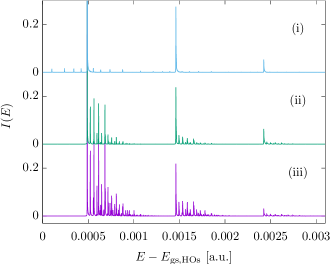
Figure 1: Morse oscillator coupled to four harmonic oscillators with $\omega_{\text{c}}=\omega_{\text{max}}=0.2\ \omega_{\text{e}}$ and $\eta_{\text{eff}}=0.2$. From top to bottom: SAM-TA-SCIVR according to Eq. (13) (blue line, (i)), M-TA-SCIVR as in Eq. (7) (green line, (ii)) and full TA-SCIVR as in Eq. (5) (violet line, (iii)). All elastic peaks are normalized to one, and the spectra overlap to make higher excitations more visible.

Results are shown in Fig. 1, where the ground state energies of the bath HOs, $E_{\text{gs},\text{HO}}=\sum_{i}\omega_{i}/2$, have been subtracted. The degree of approximation decreases from top to bottom, with SAM-TA-SCIVR according to Eq. (13) shown in blue (i), M-TA-SCIVR as in Eq. (7) in green (ii) and full TA-SCIVR as in Eq. (5) with violet lines (iii). All three approaches agree within frequency resolution in terms of peak positions. As expected and as desired, bath excitations are very much suppressed by the SAM-TA-SCIVR method. Unlike in the two reference spectra, some small ghost peaks appear in the SAM result, for example to the left of (and therefore at unphysical smaller energy than) the elastic peak. As shown analytically in App.  B for two uncoupled harmonic oscillators, these ghost peaks are second excitations of the bath modes reflected at the elastic peak. Upon close inspection, the same behavior can be observed for all higher excitations of the system. The ghost peaks are not a problem for the interpretation of the spectrum, as they are far smaller than the respective HK peak they are close to. In addition, they can be identified from their position, which is always an integer multiple of a bath frequency (or a combination thereof) to the left of a system excitation if the bath modes are sufficiently harmonic.

While the spectrum with five weakly coupled, off-resonant oscillators already contains a lot of bath excitations, all of these peaks can be assigned without difficulty. In the next example, we show a situation where this is not the case any more. The bath has still the same parameters, but now comprises 18 instead of four harmonic oscillators. We restrict the calculation to a single trajectory, which is sufficient to demonstrate the main challenge arising from this higher number of DOFs. The initial conditions are the same as before, with all DOFs centered at $(p_{\text{eq},i},q_{\text{eq},i})$. Results are shown in Fig.  2, with the SAM-TA-SCIVR result (blue line, (i)) on top, and the two reference HK calculations with different propagation times are below ((ii) and (iii)). For this higher number of bath DOFs, we see that the propagation time from the previous 5D example with $2^{15}$ steps, which leads to a numerical energy resolution $\Delta E=6\times 10^{-7}\ \text{a.u.}\ \left(0.13\ \text{cm}^{-1}\right)$, is not sufficient any more to obtain a well-resolved spectrum. This is illustrated by the reference HK calculation with this number of time steps (Fig.  2(ii), orange line), where the much higher number of bath excitations leads to a quasi-continuous spectrum that is much broader than before and does not allow for an unambiguous attribution of peaks. It is possible to recover a discrete spectrum by significantly increasing the length of the propagation and thereby the energy resolution. Results of the same reference TA-SCIVR calculation with $2^{20}$ instead of $2^{15}$ time steps are reported in the bottom spectrum of Fig.  2 (violet line, (iii)). Here, the system excitations can be seen clearly, and the bath peaks are very dense but discrete. As we go from high energy resolution in Fig.  2(iii) to the lower energy resolution in Fig.  2(ii), distinct contributions from the higher resolution can now coincide in the same energy bin. Since the density of bath peaks gets higher far away from the system excitation, as illustrated by the inset in Fig.  2, the lower resolution introduces an artificial bias that overestimates relative peak weights in these regions of high bath peak density. Conversely, the system excitations are underestimated and likely to be absorbed in the quasi-continuum. Given that the phase space integrands in Eqs. (5) and (7) are positive definite, the phase space average does not resolve this issue. Simply prolonging the propagation time, on the other hand, recreates a discrete spectrum, but this is by no means a feasible general solution, as much longer propagation times are usually prohibitively expensive and may increase the likelihood of numerical instability.

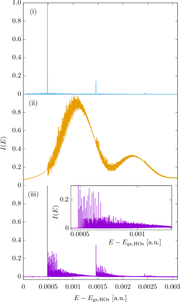
Figure 2: Morse oscillator coupled to 18 harmonic oscillators with $\omega_{\text{c}}=\omega_{\text{max}}=0.2\ \omega_{\text{e}}$ and $\eta_{\text{eff}}=0.2$. From top to bottom: SAM-TA-SCIVR according to Eq. (13) (blue line, (i)) with $2^{15}$ propagation time steps, full TA-SCIVR as in Eq. (5) with $2^{15}$ propagation time steps (orange line, (ii)), and full TA-SCIVR with $2^{20}$ propagation time steps (violet line, (iii)). The respective highest peaks are normalized to one.

Instead, the inherent filter of SAM-TA-SCIVR (blue line, (i) in Fig.  2) offers a numerically cheap solution. With the same lower number of $2^{15}$ time steps as in panel (ii), we obtain a completely different picture. By removing contributions from first-order bath excitations, the old hierarchy of prominent system peaks and very small bath excitations from Fig.  1 is restored. Compared to the higher accuracy calculation in Fig.  2(iii), it is evident that the location of the system energies is reproduced exactly. Given the higher number of bath oscillators, the number of ghost peaks is getting bigger as well. However, at least in this weakly coupled example, they are again the same order of magnitude as their accurate counterparts and therefore easily distinguished from the system excitations.

III.2 Molecular iodine embedded in krypton

Having introduced SAM-TA-SCIVR as a useful tool for the analysis of high-dimensional spectra, we now turn to an experimentally investigated system, namely, iodine in a krypton environment. Iodine surrounded by noble gas atoms has been used as a test system for a number of semiclassical approaches, for example the study of vibrational quantum coherence of iodine in argon clusters using a forward-backward IVR.Tao and Miller (2009a, b); Pan and Tao (2013) Another study of the loss of coherence of iodine in a krypton environment has already established the hybrid formalism as an appropriate tool for the investigation of this system.Buchholz et al. (2012) Here, we are interested in the change of the iodine vibrational spectrum by the surrounding krypton atoms. Experimentally, it has been found that the iodine spectrum undergoes a redshift, from gas phaseBihary et al. (2001) harmonic frequency $\omega_{\text{e}}=214.6$ $\text{cm}{}^{-1}$ and anharmonicity $\omega_{\text{e}}x_{\text{e}}=$0.627 $\text{cm}{}^{-1}$ to $\omega_{\text{e}}=211.6$ $\text{cm}{}^{-1}$ and $\omega_{\text{e}}x_{\text{e}}=$0.658 $\text{cm}{}^{-1}$ when embedded in krypton Karavitis et al. (2005), see Tab. 2.

III.2.1 Model: Dynamic Cell with Rigid Walls

As shown in a closely related investigation of iodine in an argon matrixBihary et al. (2001), there are two important caveats when it comes to spectral calculations of iodine in a rare gas environment. First, one has to choose a suitable matrix environment to reproduce the rare gas geometry faithfully, using a sufficient number of layers around the host molecule. For iodine in argon, four such layers were necessary for convergence with respect to the iodine frequency shift, corresponding to 448 argon atoms. Of these, however, only the two inner shells were taken to be mobile, while the two outer layers were fixed during the propagation; this choice of boundary conditions is called Dynamical Cell with Rigid Walls by the authors of Ref. Bihary et al., 2001. We will use the same approach, but restrict the environment to just three layers with 218 atoms for the classical geometry optimization, where the outermost is fixed and the two inner ones, comprising 72 krypton atoms, are mobile. The iodine molecule is placed inside the face-centered cubic (fcc) krypton lattice by replacing two nearest-neighbor atoms. Then, we perform a geometry optimization for the iodine as well as the mobile krypton atoms, while the outer, fixed krypton atoms serve as containment. The minimum energy geometry is presented in Fig. 3, where iodine atoms are orange and the flexible krypton atoms are blue. As a result, only a few atoms from the innermost shell are notably shifted. The subsequent normal mode analysis is performed only for the 74 flexible atoms depicted in Fig. 3 with the TrajLab software. Röblitz et al. (2014)

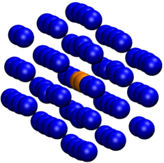
Figure 3: The iodine molecule (orange) in two flexible layers of krypton atoms (blue) after geometry optimization. Not shown is the fixed outermost layer of krypton atoms.

As a second important point, it has been demonstrated that the halogen-rare gas interaction potential is essential for getting the accurate iodine bond softening which leads to the redshift. While an anisotropic interaction of the form

$$V_{ik}(\mathbf{R}_{ik},\mathbf{R}_{12}) =\left(\cos\theta_{ik}\right)^{2}V_{\text{$\Sigma$,}ik}\left(R_{ik}\right)+\left(\sin\theta_{ik}\right)^{2}V_{\text{$\Pi$,}ik}\left(R_{ik}\right)$$ (19)

yields an even quantitatively accurate frequency shift for iodine in argon, Bihary et al. (2001) other (simpler) analytic interactions result in no shift at all or even a blueshift of the iodine frequencies. In the above equation, the index $i$ designates one of the two iodine atoms, while index $k$ stands for a krypton atom. The angle $\theta_{ik}$ is the angle between $\mathbf{R}_{ik}$ and the iodine-iodine vector $\mathbf{R}_{12}$. The total potential is modeled as a sum over two-particle interactions

$$V(\mathbf{R}_{1},\dots,\mathbf{R}_{N})= \sum_{i<j}V_{ij},$$ (20)

where we use Eq. (19) for the iodine-krypton interaction with Morse potentials $V_{\text{$\Sigma$}}$ and $V_{\Pi},$ a simple Morse potential for the iodine intramolecular interaction and a Lennard-Jones (LJ) potential for the krypton-krypton interaction. All potential parameters are collected in Tab. 1.

Morse interaction	$D_{\text{e}}\left[\text{cm}^{-1}\right]$	$s_{\text{e}}\left[\text{\r{A}}\right]$	$\alpha\left[\text{\r{A}}^{-1}\right]$
I-IBihary et al. (2001)	18357	2.666	1.536
I-Kr ($\Sigma$)Ovchinnikov and Apkarian (1996)	287	3.733	1.49
I-Kr ($\Pi$)Ovchinnikov and Apkarian (1996)	126	4.30	1.540
LJ interaction	$\epsilon\left[\text{cm}^{-1}\right]$	$\sigma\left[\text{\r{A}}\right]$
Kr-KrZadoyan et al. (1994); Ovchinnikov and Apkarian (1996)	138.7	3.58

Table 1: Parameters for the different two-particle interactions of the iodine-krypton potential.

III.2.2 Reproducing the condensed phase quantum effects by adding degrees of freedom

After geometry optimization and subsequent normal mode analysis, we find that, similar to iodine in argon, the resulting shifted harmonic frequency of the iodine vibration is already very close to the experimental result, $211.8\ \text{cm}^{-1}$ against $211.6\ \text{cm}^{-1}$. The major portion of the shift from the gas phase result $214.6\ \text{cm}^{-1}$ is thus a classical effect due to the rearrangement of iodine molecule and krypton atoms, and in particular the stretching of the iodine bond, during the geometry optimization.

In order to find the remaining contribution to the redshift due to the quantum dynamical interaction of the iodine molecule with its krypton environment and to include overtones, we perform SAM calculations with different numbers of normal coordinates included into the dynamics. We have to use $2^{17}$ semiclassical time steps with 2 classical substeps of length $\left(2\pi/\omega_{\text{e}}\right)/120$, corresponding to a frequency grid spacing of $4.4\times 10^{-7}\ \text{a.u.}$ ($0.1\ \text{cm}^{-1}$), in order to faithfully resolve possible differences. The standard phase space sampling even of a single HK DOF becoming unfeasible as the number of normal modes approaches three digits because the SAM expression (13) still requires the propagation of the full HK prefactor. Thus, the main computational challenge is the calculation of the second derivatives in normal coordinates, which brings about a computational time of a few days for one trajectory with about 100 DOFs. As a consequence, we resort to the MC-SCIVR idea that each single classical trajectory reproduces the part of the spectrum exactly that is closest to its own energy, and run only six trajectories with different initial momenta for the iodine vibrational coordinate. Each of these initial momenta corresponds to the energy of one of the first six excited states of iodine, which we can get approximately from a multiple-trajectory calculation of iodine in the rigid krypton cage.

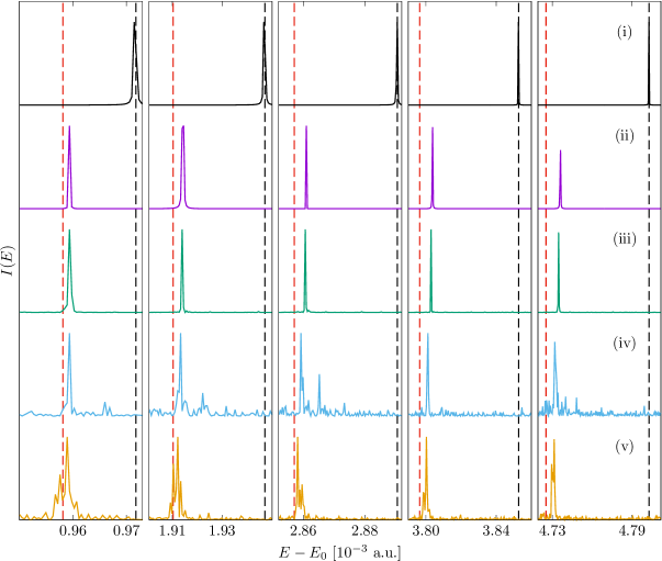
Figure 4: SAM-TA-SCIVR spectra for iodine in krypton for different numbers of normal modes included in the dynamical calculation. From left to right, the regions around the first through the fifth excited vibrational state of iodine are shown. The energy of the respective elastic peak is subtracted on the abscissa to make calculations comparable. From top to bottom: gas phase result (solid black lines, (i)), iodine vibration only in a rigid krypton cage (violet, (ii)), and spectra from calculations with 32 (green, (iii)), 60 (blue, (iv)), and 108 (orange, (v)) flexible normal modes. The dashed lines show the analytic positions of the experimental results for gas-phase iodineBihary et al. (2001) (black) and redshifted iodine in krypton Karavitis et al. (2005) (red).

Experiment	$\omega_{\text{e}}\left[\text{cm}^{-1}\right]$	$\omega_{\text{e}}x_{\text{e}}\left[\text{cm}^{-1}\right]$
gas phase $\text{I}_{2}$Bihary et al. (2001)	214.6	0.627
$\text{I}_{2}$ in KrKaravitis and Apkarian (2004)	211.3	0.652
$\text{I}_{2}$ in KrKaravitis et al. (2005)	211.6	0.658
Numerical results	$\omega_{\text{e}}\left[\text{cm}^{-1}\right]$	$\omega_{\text{e}}x_{\text{e}}\left[\text{cm}^{-1}\right]$
normal mode analysis	211.8	–
$\text{I}_{2}$ vibration in rigid Kr cage	211.8	0.62
32 DOFs	211.8	0.63
60 DOFs	211.7	0.64
108 DOFs	211.6	0.63

Table 2: Spectroscopic parameters of the molecular iodine Morse potential. All numerical results have been obtained from Birge-Sponer fits to the first six iodine eigenenergies from the SAM-TA-SCIVR spectrum. The number of DOFs indicates how many of the 216 internal DOFs of the two-shell iodine-krypton cluster have been considered in the dynamics.

In our SAM calculations, which are summarized in Fig. 4 and Tab. 2, we always treat the iodine vibration as the only HK DOF. The first calculation (solid violet line, (ii), in Fig. 4) comprises only this one DOF, i.e. all krypton atoms are rigid. All excited peaks from the five single-trajectory calculations are very clean, as there are only iodine excitations in the respective spectra. A Birge-Sponer fit reveals that the harmonic frequency is indeed identical to the eigenvalue of the normal mode, as shown in Tab. 2. The anharmonicity $x_{\text{e}}\omega_{\text{e}}$ is clearly closer to the gas phase result than to the redshifted result in krypton. Increasing the dimensionality of the system, we now take into account all 32 fully symmetric normal modes (green lines, (iii), in Fig. 4). All bath DOFs carry initial momentum corresponding to the harmonic frequency of the respective mode. We thus need to employ the SAM filter, which works as intended in fully removing all bath excitations at least in close proximity to the system peaks. These peaks are already shifted a little bit towards the redshifted experimental result, which is also reflected in the results of the Birge-Sponer fit. By adding more normal modes to the dynamical calculation, we can see that this trend continues. With 59 TG normal modes with the same initial excitation as before (blue lines, (iv)), we still find system peaks that can clearly be identified as such, but also a certain amount of noise that is no longer filtered out completely. The growing number of normal modes influencing the dynamics of the iodine vibration causes another quite significant shift towards the experimental result.

Going up to include 108 normal modes, we finally approach the limits of SAM. We have given only 60 modes initial excitation corresponding to the respective mode’s ground state energy $\omega_{i}$ while the remaining modes have zero initial momentum. Higher initial energy of the remaining bath DOFs would bring about significant excitation of some higher order bath states, such that the corresponding peaks are not filtered sufficiently by the SAM approach any more. In spite of this limitation, we still see an improvement of the excited peak positions in the case of 108 normal modes (orange lines, (v), in Fig. 4). This also shows in the fitted value for $\omega_{\text{e}}$, which is closest to the experimental results (Tab. 2).

IV Conclusions and Outlook

In this work, we have presented a simplified version of the mixed time-averaging SCIVR. The underlying idea of M-TA-SCIVR is a hybrid description of phase space, where a small part is described on the HK level of accuracy, while the remaining environment is treated with TG. The SAM-TA-SCIVR builds upon this idea, but takes another approximative step by using the exact harmonic oscillator results for the TG part of the phase space integrand. This leads to a considerably simplified expression, reminiscent of the original HK TA-SCIVR with a reduced phase space sampling. The motivation for this approximation was to find an approach that is still accurate for the HK DOFs, but at the same time removes bath excitations from the spectrum.

In the application to a Morse oscillator coupled to a Caldeira-Leggett bath, we have seen for a small number of bath degrees of freedom that SAM indeed reproduces the HK peaks on the same level of accuracy as reference HK or mixed calculations. The decisive advantage over the formally more accurate approaches is the removal of odd harmonics of the bath oscillators. For twenty bath oscillators, this filter effect proved its value by recreating a clear spectrum from the same classical dynamics that yields excessively noisy spectra with the reference methods. The only unfavorable characteristic of the SAM spectra are some ghost peaks from the environmental DOFs. Since these ghost peaks are both very small and appear at well-understood positions, we do not consider them a problem for the applicability of the method.

Investigating an experimentally studied problem, namely, the redshift of the iodine molecule embedded in a krypton environment, we first saw that the shift of the harmonic approximation frequency $\omega_{\text{e}}$ of the iodine Morse potential is mainly an effect resulting from the rearrangement of iodine and krypton atoms in a classical geometry optimization. We then used SAM to find the effect of the krypton environment on the excited iodine vibrational energies and to see the change in iodine energies due to the dynamical interaction with the environment. The SAM approach allowed to include up to 108 vibrational DOFs in the calculation, where either all or at least the majority of the bath modes carry initial excitation. In spite of all interactions in this system being anharmonic, the bath filter still works as intended and we can easily identify the system excitations. In the model with two flexible inner krypton shells, contained by a fixed outer layer, we could show that adding more and more normal modes to the calculation systematically improves the result towards very good quantitative agreement with experimental findings. Thus, the increasingly complex environment appropriately captures the effect of the system-bath dynamics on the iodine spectrum, both for the fundamental frequency and the overtones.

In the future, the SAM approach will be combined with Divide-and-Conquer SCIVRCeotto et al. (2017); Liberto et al. (2018) for tackling condensed phase systems using ab initio potentials. This combination of methods will allow the system to be significantly higher in dimensionality since the SAM approach properly embeds the system into a condensed phase environment.

V Acknowledgements

Michele Ceotto and Max Buchholz acknowledge financial support from the European Research Council (ERC) under the European Union’s Horizon 2020 research and innovation programme (Grant Agreement No. [647107] — SEMICOMPLEX — ERC-2014-CoG). M.C. acknowledges also the CINECA and the Regione Lombardia award under the LISA initiative (grant GREENTI) for the availability of high performance computing resources. M.B. would like to thank his son for providing the acronym for the method proposed in this paper.

Appendix A Quantities From the Separable Mixed Expression

For this paper to be self-contained, we briefly collect the terms from the separable mixed approximation in Eq.  (7) that have not been defined in the main text. The $2F_{\text{tg}}\times 2F_{\text{tg}}$ matrix $\mathbf{A}(t)$, which collects coefficients of the quadratic deviations from the TG initial conditions, consists of four submatrices defined asBuchholz et al. (2017)

$$\begin{split}\mathbf{A}_{11}(t)=&\frac{1}{4}\mathbf{m}_{21}^{\text{T}}\left(t\right)\mathbf{\boldsymbol{\gamma}}\mathbf{m}_{21}\left(t\right)+\frac{1}{4\hbar^{2}}\mathbf{m}_{11}^{\text{T}}\left(t\right)\mathbf{\boldsymbol{\gamma}}^{-1}\mathbf{m}_{11}\left(t\right)\\ \mathbf{A}_{12}(t)=&\frac{1}{4}\mathbf{m}_{21}^{\text{T}}\left(t\right)\boldsymbol{\gamma}\mathbf{m}_{22}\left(t\right)+\frac{1}{4\hbar^{2}}\mathbf{m}_{11}^{\text{T}}\left(t\right)\boldsymbol{\gamma}^{-1}\mathbf{m}_{12}\left(t\right)\\ \mathbf{A}_{21}(t)=&\frac{1}{4}\mathbf{m}_{22}^{\text{T}}\left(t\right)\boldsymbol{\gamma}\mathbf{m}_{21}\left(t\right)+\frac{1}{4\hbar^{2}}\mathbf{m}_{12}^{\text{T}}\left(t\right)\boldsymbol{\gamma}^{-1}\mathbf{m}_{11}\left(t\right)\\ \mathbf{A}_{22}(t)=&\frac{1}{4}\mathbf{m}_{22}^{\text{T}}\left(t\right)\boldsymbol{\gamma}\mathbf{m}_{22}\left(t\right)+\frac{1}{4\hbar^{2}}\mathbf{m}_{12}^{\text{T}}\left(t\right)\mathbf{\boldsymbol{\gamma}}^{-1}\mathbf{m}_{12}\left(t\right).\end{split}$$ (21)

Prefactors of terms linear in the deviations are summarized in the $2F_{\text{tg}}$-dimensional vector $\mathbf{b}(t)\equiv\left(\mathbf{b}_{1,t}^{\text{T}},\mathbf{b}_{2,t}^{\text{T}}\right)^{\text{T}}$ with subvectors

$$\begin{split}\mathbf{b}_{1,t}^{\text{T}}=&-\frac{1}{2}\left(\mathbf{q}\left(t\right)-\mathbf{q}\left(0\right)\right)^{\text{T}}\left[\mathbf{\boldsymbol{\gamma}}\mathbf{m}_{21}\left(t\right)+\frac{\text{i}}{\hbar}\mathbf{m}_{11}\left(t\right)\right]\\ &-\frac{1}{2\hbar^{2}}\left(\mathbf{p}\left(t\right)-\mathbf{p}\left(0\right)\right)^{\text{T}}\left[\mathbf{\boldsymbol{\gamma}}^{-1}\mathbf{m}_{11}\left(t\right)-\text{i}\hbar\mathbf{m}_{21}\left(t\right)\right]\\ \mathbf{b}_{2,t}^{\text{T}}=&-\frac{1}{2}\left(\mathbf{q}\left(t\right)-\mathbf{q}\left(0\right)\right)^{\text{T}}\left[\mathbf{\boldsymbol{\gamma}}\mathbf{m}_{22}\left(t\right)+\frac{\text{i}}{\hbar}\mathbf{m}_{12}\left(t\right)\right]\\ &-\frac{1}{2\hbar^{2}}\left(\mathbf{p}\left(t\right)-\mathbf{p}\left(0\right)\right)^{\text{T}}\left[\mathbf{\boldsymbol{\gamma}}^{-1}\mathbf{m}_{12}\left(t\right)-\text{i}\hbar\mathbf{m}_{22}\left(t\right)\right],\end{split}$$ (22)

where we remind the reader that $\left(\mathbf{p}(t),\mathbf{q}(t)\right)$ is the trajectory starting at the mixed initial conditions $\left(\mathbf{p}(0),\mathbf{q}(0)\right)$ from Eq.  (6). The $\mathbf{m}_{ij}$ in the two above equations are non-square $F\times F_{\text{tg}}$ submatrices of the stability matrix,

$$\begin{split}\mathbf{m}_{11}(t)=&\frac{\partial\mathbf{p}(t)}{\partial\mathbf{p}_{\text{tg}}(0)},\quad\mathbf{m}_{12}(t)=\frac{\partial\mathbf{p}(t)}{\partial\mathbf{q}_{\text{\text{tg}}}(0)},\\ \mathbf{m}_{21}(t)=&\frac{\partial\mathbf{q}(t)}{\partial\mathbf{p}_{\text{tg}}(0)},\quad\mathbf{m}_{22}(t)=\frac{\partial\mathbf{q}(t)}{\partial\mathbf{q}_{\text{\text{tg}}}(0)}.\end{split}$$ (23)

Assuming, for simplicity, a system of two uncoupled harmonic oscillators with equations of motion

$$\begin{split}p_{i}(t)&=p_{\text{eq},i}\cos\omega_{i}t-m_{i}\omega_{i}q_{\text{eq},i}\sin\omega_{i}t\\ q_{i}(t)&=q_{\text{eq},i}\cos\omega_{i}t+\frac{p_{\text{eq},i}}{m_{i}\omega_{i}}\sin\omega_{i}t,\end{split}$$ (24)

and treating site 1 with HK and site 2 on the TG level, we get zero for the respective first component of the stability submatrices, $m_{ij,1}=0$, and the second components amount to

$$\begin{split}m_{11,2}(t)=&\cos\omega_{2}t,\quad m_{12,2}(t)=-m_{2}\omega_{2}\sin\omega_{2}t,\\ m_{21,2}(t)=&\sin\omega_{2}t/(m_{2}\omega_{2}),\quad m_{22,2}(t)=\cos\omega_{2}t.\end{split}$$ (25)

With the usual $\gamma_{i}=m_{i}\omega_{i}/\hbar$, the matrix $\mathbf{A}$ becomes time independent,

$$\mathbf{A}=\frac{1}{4}\left(\begin{array}[]{cc}1/(\hbar m_{2}\omega_{2})&0\\ 0&m_{2}\omega_{2}/\hbar\end{array}\right).$$ (28)

We thus find for this single uncoupled TG DOF

$$\frac{1}{\left[\det\left(\mathbf{A}\left(t\right)+\mathbf{A}^{*}\left(t\right)\right)\right]^{1/4}} =\left(2\hbar\right)^{1/2},$$ (29)

and this result can be easily generalized to the case of $F_{\text{tg}}$ uncoupled HOs to yield Eq. (9). With the inverse

$$\left(\mathbf{A}\left(t\right)+\mathbf{A}^{*}\left(t\right)\right)^{-1} =\left(\begin{array}[]{cc}2\hbar m_{2}\omega_{2}&0\\ 0&2\hbar/\left(m_{2}\omega_{2}\right)\end{array}\right)$$ (32)

and the relation

$$b_{2,t} =-\text{i}m_{2}\omega_{2}b_{1,t},$$ (33)

we obtain the one-dimensional case of Eq. (10),

$$\mathbf{b}_{t}^{\text{T}}\left(\mathbf{A}\left(t\right)+\mathbf{A}^{*}\left(t\right)\right)^{-1}\mathbf{b}_{t} =2\hbar m_{2}\omega_{2}b_{1,t}^{2}+\frac{2\hbar}{m_{2}\omega_{2}}\left(\text{i}m_{2}\omega_{2}\right)^{2}b_{1,t}^{2}=0.$$ (34)

All of these results will be used in the application of SAM-TA-SCIVR to the calculation of the spectrum of two uncoupled HOs in App. B.

Appendix B Analytical Application of SAM-TA-SCIVR to Two Uncoupled Harmonic Oscillators

The dynamics of two uncoupled HOs of unit mass with frequencies $\omega_{1}$ and $\omega_{2}$, respectively, is described by the Hamiltonian (in atomic units)

$$H =\frac{p_{1}^{2}}{2}+\frac{p_{2}^{2}}{2}+\frac{\omega_{1}^{2}q_{1}^{2}}{2}+\frac{\omega_{2}^{2}q_{2}^{2}}{2}.$$ (35)

The exact result for the spectrum, which can be found analytically as the product of two TA-SCIVR spectra,Ceotto et al. (2009a) reads

$$I_{\text{HK}}(E)=\exp\left[-\frac{p_{\text{eq,1}}^{2}}{2\hbar\omega_{1}}\right]\exp\left[-\frac{p_{2,0}^{2}}{2\hbar\omega_{2}}\right]$$

$$\times\sum\limits_{n,m}\frac{1}{2^{n+m}n!m!}\left(\frac{p_{\text{eq,1}}^{2}}{\hbar\omega_{1}}\right)^{n}\left(\frac{p_{\text{eq,2}}^{2}}{\hbar\omega_{2}}\right)^{m}\delta\left(E-\hbar\omega_{1}\left[n+\frac{1}{2}\right]-\hbar\omega_{2}\left[m+\frac{1}{2}\right]\right),$$ (36)

where initial conditions $(\mathbf{p}_{\text{eq}},\mathbf{0})$ have been chosen for simplicity and $\hbar$ has been set to unity. Using M-TA-SCIVR according to Eq. (7) instead and treating the HO with index “1” with HK while describing the HO with index “2” on the TG level, Buchholz et al. (2016) the result looks very similar

$$I_{\text{M}}(E)=\exp\left[-\frac{p_{\text{eq,1}}^{2}}{2\hbar\omega_{1}}\right]\exp\left[-\frac{p_{\text{eq,2}}^{2}}{\hbar\omega_{2}}\right]$$

$$\times\sum\limits_{n,m}\frac{1}{2^{n+2m}n!(m!)^{2}}\left(\frac{p_{\text{eq,1}}^{2}}{\hbar\omega_{1}}\right)^{n}\left(\frac{p_{\text{eq,2}}^{2}}{\hbar\omega_{2}}\right)^{2m}\delta\left(E-\hbar\omega_{1}\left[n+\frac{1}{2}\right]-\hbar\omega_{2}\left[m+\frac{1}{2}\right]\right).$$ (37)

With the mixed approach, all peaks positions of the TG coordinate are reproduced exactly, while the peak weights are changed such that overtones are suppressed. Buchholz et al. (2016) While this inherent suppression is a nice feature, it is not enough to completely remove peaks from a very noisy spectrum, as we have seen in Fig. 2.

We will therefore apply the SAM-TA-SCIVR to this problem, using the same phase space separation as before. As in the analytic results above, we will set the initial position to zero for notational brevity, and replace $p_{\text{\text{hk}}}(0)$ with $p_{1}$ as well as $\left(p_{\text{eq},\text{hk}},p_{\text{eq},\text{tg}}\right)$ with $\left(p_{\text{eq},1},p_{\text{eq,2}}\right)$ for the same reason. After unfolding the modulus in Eq. (13), the SAM formulation thus becomes

$$I(E)= \ \frac{1}{2\pi\hbar}\frac{1}{\pi\hbar T}\int\text{d}p_{1}\int\text{d}q_{1}\text{Re}\Bigg{\{}\int_{0}^{T}\text{d}t_{1}\int_{t_{1}}^{\infty}\text{d}t_{2}$$

$$\times\text{e}^{\text{i}\left[E\left(t_{2}-t_{1}\right)+\phi\left(t_{2}\right)-\phi\left(t_{1}\right)+S\left(t_{2}\right)-S\left(t_{1}\right)\right]/\hbar}$$

$$\times\left\langle p_{\text{eq,1}},0\middle|p_{1}\left(t_{2}\right),q_{1}\left(t_{2}\right)\right\rangle\left\langle p_{1}\left(t_{1}\right),q_{1}\left(t_{1}\right)\middle|p_{\text{eq,1}},0\right\rangle\Bigg{\}},$$ (38)

where $\left(p_{1}\left(t\right),q_{1}\left(t\right)\right)$ is the classical trajectory from Eq. (24). Using the classical trajectory with $\mathbf{q}_{0}=\mathbf{0}$, the action becomes

$$S(t) =\left(\frac{p_{1}^{2}}{2\omega_{1}}-\frac{1}{2}\omega_{1}q_{1}^{2}\right)\cos\omega_{1}t\sin\omega_{1}t-p_{1}q_{1}\text{sin}^{2}\omega_{1}t+\frac{p_{\text{eq,2}}^{2}}{2\omega_{2}}\cos\omega_{2}t\sin\omega_{2}t,$$ (39)

and the prefactor phase is

$$\phi\left(t\right) =-\frac{\hbar\left(\omega_{1}+\omega_{2}\right)}{2}t.$$ (40)

The phase space integration over the HK coordinates can be performed analytically, and the remaining time integrand in Eq. (38) can be written in the form of a large exponential,

$$\exp\left\{\frac{\text{i}}{\hbar}\left[E\left(t_{2}-t_{1}\right)+\phi(t_{2})-\phi(t_{1})\right]+E_{\text{hk}}\left(t_{1},t_{2}\right)+E_{\text{tg}}\left(t_{1},t_{2}\right)\right\}$$ , (41)

where the term $E_{\text{hk}}\left(t_{1},t_{2}\right)$ denotes the phase space integrated contribution from the HK DOF,Ceotto et al. (2009a); Buchholz et al. (2016) and $E_{\text{tg}}\left(t_{1},t_{2}\right)$ is the contribution of the TG part, which consists only of (part of) the action. Taking results from Refs.  Ceotto et al., 2009a and Buchholz et al., 2016 and changing the integration variables to $\tau=t_{2}-t_{1}$ and $\tau^{\prime}=t_{1}$, the HK term becomes

$$E_{\text{hk}}\left(\tau,\tau^{\prime}\right) =\frac{p_{\text{eq},1}^{2}}{2\hbar\omega_{1}}\left(\text{e}^{-\text{i}\omega_{1}\tau}-1\right).$$ (42)

For the TG term, we replace the trigonometric functions by exponentials to find

$$E_{\text{tg}}\left(\tau,\tau^{\prime}\right) =\frac{1}{4\hbar}\frac{p_{\text{eq,2}}^{2}}{2\omega_{2}}\left[\text{e}^{2\text{i}\omega_{2}\left(\tau+\tau^{\prime}\right)}-\text{e}^{-2\text{i}\omega_{2}\left(\tau+\tau^{\prime}\right)}-\text{e}^{2\text{i}\omega_{2}\tau^{\prime}}+\text{e}^{-2\text{i}\omega_{2}\tau^{\prime}}\right]$$ (43)

This makes the intermediate expression for the SAM spectrum

$$I(E)= \ \frac{1}{\pi\hbar T}\text{e}^{-p_{\text{eq},1}^{2}/\left(2\hbar\omega_{1}\right)}\text{Re}\Bigg{\{}\int_{0}^{T}\text{d}\tau^{\prime}\int_{0}^{\infty}\text{d}\tau\ \text{e}^{\text{i}\left[E-\hbar\left(\omega_{1}+\omega_{2}\right)/2\right]\tau/\hbar}$$

$$\times\exp\left\{\frac{p_{\text{eq,1}}^{2}}{2\hbar\omega_{1}}\text{e}^{-\text{i}\omega_{1}\tau}+\frac{1}{4}\frac{p_{\text{eq,2}}^{2}}{2\hbar\omega_{2}}\left[\text{e}^{2\text{i}\omega_{2}\left(\tau+\tau^{\prime}\right)}-\text{e}^{-2\text{i}\omega_{2}\left(\tau+\tau^{\prime}\right)}+\text{e}^{-2\text{i}\omega_{2}\tau^{\prime}}-\text{e}^{2\text{i}\omega_{2}\tau^{\prime}}\right]\right\}\Bigg{\}}.$$ (44)

We can now write the exponential in the last line as a product with five factors and replace the lower exponentials by their power series expansionsCeotto et al. (2009a); Buchholz et al. (2016)

$$I(E)= \ \frac{1}{\pi\hbar T}\text{e}^{-p_{\text{eq,1}}^{2}/\left(2\hbar\omega_{1}\right)}\text{Re}\Bigg{\{}\int_{0}^{T}\text{d}\tau^{\prime}\int_{0}^{\infty}\text{d}\tau\ \text{e}^{\text{i}\left[E-\hbar\left(\omega_{1}+\omega_{2}\right)/2\right]\tau/\hbar}$$

$$\times\sum_{n,m,k,l,o}\frac{\left(-1\right)^{k+o}}{n!m!k!l!o!}\left(\frac{p_{\text{eq,1}}^{2}}{2\hbar\omega_{1}}\right)^{n}\left(\frac{1}{4}\frac{p_{\text{eq,2}}^{2}}{2\hbar\omega_{2}}\right)^{m+k+l+o}\text{e}^{-\text{i}\omega_{1}n\tau}\text{e}^{2\text{i}\omega_{2}m\left(\tau+\tau^{\prime}\right)}\text{e}^{-2\text{i}\omega_{2}k\left(\tau+\tau^{\prime}\right)}\text{e}^{-2\text{i}l\omega_{2}\tau^{\prime}}\text{e}^{2\text{i}o\omega_{2}\tau^{\prime}}\Bigg{\}}.$$ (45)

The resulting fivefold sum collapses to a sum over three variables in the limit $T\rightarrow\infty$ because the factor $1/T$ needs to cancel after integration over $\tau^{\prime}$ in order for the contribution to survive, which is the case only for $k=o$ and $l=m$, and we end up with

$$I(E)= \ \frac{1}{\pi\hbar}\text{e}^{-p_{\text{eq,1}}^{2}/\left(2\hbar\omega_{1}\right)}\text{Re}\Bigg{\{}\int_{0}^{\infty}\text{d}\tau\ \text{e}^{\text{i}\left[E-\hbar\left(\omega_{1}+\omega_{2}\right)/2\right]\tau/\hbar}$$

$$\times\sum_{n,k,l}\frac{1}{n!\left(k!l!\right)^{2}}\left(\frac{p_{\text{eq,1}}^{2}}{2\hbar\omega_{1}}\right)^{n}\left(\frac{1}{4}\frac{p_{\text{eq,2}}^{2}}{2\hbar\omega_{2}}\right)^{2k+2l}\exp\left[-\text{i}\omega_{1}n\tau-2\text{i}\omega_{2}\left(k-l\right)\tau\right]\Bigg{\}}.$$ (46)

After performing the remaining integration over $\tau$, the final SAM spectrum for two uncoupled HOs emerges as

$$I_{\text{SAM}}(E)=\exp\left[-\frac{p_{\text{eq,1}}^{2}}{2\hbar\omega_{1}}\right]$$

$$\times\sum\limits_{n,k,l}\frac{1}{2^{n}2^{3(2k+2l)}}\frac{1}{n!(k!)^{2}(l!)^{2}}\left(\frac{p_{\text{eq,1}}^{2}}{\hbar\omega_{1}}\right)^{n}\left(\frac{p_{\text{eq,2}}^{2}}{\hbar\omega_{2}}\right)^{2k+2l}\delta\left(E-\hbar\omega_{1}\left[n+\frac{1}{2}\right]-\hbar\omega_{2}\left[2(k-l)+\frac{1}{2}\right]\right)$$ (47)

From the comparison to the exact and mixed results in Eqs. (36) and (37), we get an insight into the nature of this approximation. First, setting $n=k=l=0$, the correct ground state energy of the composed system is recovered. Second, by comparing the case $k=l=0$ in Eq. (47) to $m=0$ in the other expressions, we find all three spectra for the HK DOF to be exactly the same. Third, the SAM expression turns out to contain only even peaks in the TG coordinate. This is an important property given that these DOFs are usually centered around the ground state energy initially, which means that the first excitations are the main source of unwanted, noisy peaks. Finally, we see that all even TG excitations have an unphysical counterpart at the respective “negative frequency”. The correct second excitation at $\omega_{1}+5\omega_{2}/2$ ($n=l=0$, $k=1$), for example, has a ghost peak equivalent at $\omega_{1}-5\omega_{2}/2$ ($n=k=0$, $l=1$). However, all TG peaks are systematically much smaller than the closest HK peaks. This is why we think that the ghost peaks are a small price to pay for a cheap built-in filter that removes odd TG excitations and thus makes spectra accessible that would be just noise otherwise. In the numerical examples in Sec. III, we show that these properties hold approximately also for anharmonic, coupled systems.

References

- Miller (1968) W. H. Miller, J. Chem. Phys. 48, 464 (1968).
- Wolken Jr et al. (1972) G. Wolken Jr, W. H. Miller, and M. Karplus, J. Chem. Phys. 56, 4930 (1972).
- Garrett and Miller (1978) B. C. Garrett and W. H. Miller, J. Chem. Phys. 68, 4051 (1978).
- Miller (1971) W. H. Miller, Accounts of Chemical Research 4, 161 (1971).
- Bowman and Lee (1980) J. M. Bowman and K. T. Lee, J. Chem. Phys. 72, 5071 (1980).
- Bowman and Kupperman (1973) J. Bowman and A. Kupperman, Chem. Phys. 2, 158 (1973).
- Schatz et al. (1975) G. C. Schatz, J. M. Bowman, and A. Kuppermann, J. Chem. Phys. 63, 674 (1975).
- Gianturco (1976) F. Gianturco, International Journal of Quantum Chemistry 10, 37 (1976).
- Aquilanti and Casavecchia (1976) V. Aquilanti and P. Casavecchia, J. Chem. Phys. 64, 751 (1976).
- Aquilanti and Laganà (1975) V. Aquilanti and A. Laganà, Zeitschrift für Physikalische Chemie 96, 229 (1975).
- Bonnet and Rayez (1997) L. Bonnet and J. Rayez, Chem. Phys. Lett. 277, 183 (1997).
- Aquilanti et al. (2000) V. Aquilanti, A. Beddoni, S. Cavalli, A. Lombardi, and R. Littlejohn, Molecular Physics 98, 1763 (2000).
- Connor et al. (1979) J. Connor, W. Jakubetz, and A. Lagana, Journal of Physical Chemistry 83, 73 (1979).
- De Fazio et al. (1994) D. De Fazio, F. Gianturco, J. Rodriguez-Ruiz, K. Tang, and J. Toennies, Journal of Physics B: Atomic, Molecular and Optical Physics 27, 303 (1994).
- Miller et al. (2003) W. H. Miller, Y. Zhao, M. Ceotto, and S. Yang, J. Chem. Phys. 119, 1329 (2003).
- Ceotto and Miller (2004) M. Ceotto and W. H. Miller, J. Chem. Phys. 120, 6356 (2004).
- Ceotto et al. (2005) M. Ceotto, S. Yang, and W. H. Miller, J. Chem. Phys. 122, 044109 (2005).
- Aieta and Ceotto (2017) C. Aieta and M. Ceotto, J. Chem. Phys. 146, 214115 (2017).
- Aieta et al. (2016) C. Aieta, F. Gabas, and M. Ceotto, J. Phys. Chem. A 120, 4853 (2016).
- Mandrà et al. (2013) S. Mandrà, S. Valleau, and M. Ceotto, International Journal of Quantum Chemistry 113, 1722 (2013).
- Mandrà et al. (2014) S. Mandrà, J. Schrier, and M. Ceotto, J. Phys. Chem. A 118, 6457 (2014).
- Conte et al. (2015a) R. Conte, P. L. Houston, and J. M. Bowman, J. Phys. Chem. A 119, 12304 (2015a).
- Conte et al. (2015b) R. Conte, C. Qu, and J. M. Bowman, J. Chem. Theory Comput. 11, 1631 (2015b).
- Homayoon et al. (2015) Z. Homayoon, R. Conte, C. Qu, and J. M. Bowman, J. Chem. Phys. 143, 084302 (2015).
- Houston et al. (2016) P. L. Houston, R. Conte, and J. M. Bowman, J. Phys. Chem. A 120, 5103 (2016).
- Qu et al. (2015) C. Qu, R. Conte, P. L. Houston, and J. M. Bowman, Phys. Chem. Chem. Phys. 17, 8172 (2015).
- Conte et al. (2014) R. Conte, P. L. Houston, and J. M. Bowman, J. Chem. Phys. 140, 151101 (2014).
- Conte et al. (2013a) R. Conte, P. L. Houston, and J. M. Bowman, J. Phys. Chem. A 117, 14028 (2013a).
- Feynman and Hibbs (1965) R. P. Feynman and A. R. Hibbs, Quantum mechanics and path integrals (McGraw-Hill, 1965).
- Ceperley (1995) D. M. Ceperley, Rev. Mod. Phys. 67, 279 (1995).
- Parrinello and Rahman (1984) M. Parrinello and A. Rahman, J. Chem. Phys. 80, 860 (1984).
- Marx and Parrinello (1996) D. Marx and M. Parrinello, J. Chem. Phys. 104, 4077 (1996).
- Tuckerman et al. (1996) M. E. Tuckerman, D. Marx, M. L. Klein, and M. Parrinello, J. Chem. Phys. 104, 5579 (1996).
- Cao and Voth (1994) J. Cao and G. A. Voth, J. Chem. Phys. 100, 5093 (1994).
- Geva et al. (2001) E. Geva, Q. Shi, and G. A. Voth, J. Chem. Phys. 115, 9209 (2001).
- Paesani et al. (2009) F. Paesani, S. S. Xantheas, and G. A. Voth, J. Phys. Chem. B 113, 13118 (2009).
- Poulsen and Rossky (2001) J. A. Poulsen and P. J. Rossky, J. Chem. Phys. 115, 8024 (2001).
- Habershon et al. (2013) S. Habershon, D. E. Manolopoulos, T. E. Markland, and T. F. Miller III, Annu. Rev. Phys. Chem. 64, 387 (2013).
- Craig and Manolopoulos (2005a) I. R. Craig and D. E. Manolopoulos, J. Chem. Phys. 122, 084106 (2005a).
- Craig and Manolopoulos (2005b) I. R. Craig and D. E. Manolopoulos, J. Chem. Phys. 123, 034102 (2005b).
- Habershon et al. (2007) S. Habershon, B. J. Braams, and D. E. Manolopoulos, J. Chem. Phys. 127, 174108 (2007).
- Markland and Manolopoulos (2008) T. E. Markland and D. E. Manolopoulos, J. Chem. Phys. 129, 024105 (2008).
- Richardson and Althorpe (2009) J. O. Richardson and S. C. Althorpe, J. Chem. Phys. 131, 214106 (2009).
- Suleimanov et al. (2011) Y. V. Suleimanov, R. Collepardo-Guevara, and D. E. Manolopoulos, J. Chem. Phys. 134, 044131 (2011).
- Menzeleev et al. (2011) A. R. Menzeleev, N. Ananth, and T. F. Miller III, J. Chem. Phys. 135, 074106 (2011).
- Ananth (2013) N. Ananth, J. Chem. Phys. 139, 124102 (2013).
- Shakib and Huo (2017) F. A. Shakib and P. Huo, J. Phys. Chem. Lett. 8, 3073 (2017).
- Witt et al. (2009) A. Witt, S. D. Ivanov, M. Shiga, H. Forbert, and D. Marx, J. Chem. Phys. 130, 194510 (2009).
- Rossi et al. (2014) M. Rossi, M. Ceriotti, and D. E. Manolopoulos, J. Chem. Phys. 140, 234116 (2014).
- Miller (2006) W. H. Miller, J. Chem. Phys. 125, 132305 (2006).
- Heller (1975) E. J. Heller, J. Chem. Phys. 62, 1544 (1975).
- Kay (2005) K. G. Kay, Annu. Rev. Phys. Chem. 56, 255 (2005).
- Thoss and Wang (2004) M. Thoss and H. Wang, Annu. Rev. Phys. Chem. 55, 299 (2004).
- Walton and Manolopoulos (1996) A. R. Walton and D. E. Manolopoulos, Mol. Phys. 87, 961 (1996).
- Walton and Manolopoulos (1995) A. R. Walton and D. E. Manolopoulos, Chem. Phys. Lett. 244, 448 (1995).
- Pollak (2007) E. Pollak, “The Semiclassical Initial Value Series Representation of the Quantum Propagator,” in Quantum Dynamics of Complex Molecular Systems, edited by D. A. Micha and I. Burghardt (Springer Berlin Heidelberg, Berlin, Heidelberg, 2007) pp. 259–271.
- Bonella et al. (2005) S. Bonella, D. Montemayor, and D. F. Coker, Proc. Natl. Acad. Sci. 102, 6715 (2005).
- Huo and Coker (2012) P. Huo and D. F. Coker, Mol. Phys. 110, 1035 (2012).
- Miller (2001a) W. H. Miller, J. Phys. Chem. A 105, 2942 (2001a).
- Miller (2005) W. H. Miller, Proc. Natl. Acad. Sci. USA 102, 6660 (2005).
- Kay (1994a) K. G. Kay, J. Chem. Phys. 101, 2250 (1994a).
- Kay (1994b) K. G. Kay, J. Chem. Phys. 100, 4432 (1994b).
- Heller (1981a) E. J. Heller, J. Chem. Phys. 75, 2923 (1981a).
- Wang et al. (1998) H. Wang, X. Sun, and W. H. Miller, J. Chem. Phys. 108, 9726 (1998).
- Yamamoto et al. (2002) T. Yamamoto, H. Wang, and W. H. Miller, J. Chem. Phys. 116, 7335 (2002).
- Conte and Pollak (2012) R. Conte and E. Pollak, J. Chem. Phys. 136, 094101 (2012).
- Conte and Pollak (2010) R. Conte and E. Pollak, Phys. Rev. E 81, 036704 (2010).
- Berry and Mount (1972) M. V. Berry and K. Mount, Rep. on Prog. Phys. 35, 315 (1972).
- Wang et al. (2000) H. Wang, M. Thoss, and W. H. Miller, J. Chem. Phys. 112, 47 (2000).
- Wang et al. (2001) H. Wang, M. Thoss, K. L. Sorge, R. Gelabert, X. Giménez, and W. H. Miller, J. Chem. Phys. 114, 2562 (2001).
- Zhuang et al. (2012) Y. Zhuang, M. R. Siebert, W. L. Hase, K. G. Kay, and M. Ceotto, J. Chem. Theory Comput. 9, 54 (2012).
- Ceotto et al. (2017) M. Ceotto, G. Di Liberto, and R. Conte, Phys. Rev. Lett. 119, 010401 (2017).
- Gabas et al. (2017) F. Gabas, R. Conte, and M. Ceotto, J. Chem. Theory Comput. 13, 2378 (2017).
- Monteferrante et al. (2013) M. Monteferrante, S. Bonella, and G. Ciccotti, J. Chem. Phys. 138, 054118 (2013).
- Bonella et al. (2010) S. Bonella, G. Ciccotti, and R. Kapral, Chem. Phys. Lett. 484, 399 (2010).
- Pollak and Martin-Fierro (2007) E. Pollak and E. Martin-Fierro, J. Chem. Phys. 126, 164107 (2007).
- Wehrle et al. (2015) M. Wehrle, S. Oberli, and J. Vaníček, J. Phys. Chem. A 119, 5685 (2015).
- Wehrle et al. (2014) M. Wehrle, M. Sulc, and J. Vanicek, J. Chem. Phys. 140, 244114 (2014).
- Ceotto et al. (2009a) M. Ceotto, S. Atahan, G. F. Tantardini, and A. Aspuru-Guzik, J. Chem. Phys. 130, 234113 (2009a).
- Ceotto et al. (2009b) M. Ceotto, S. Atahan, S. Shim, G. F. Tantardini, and A. Aspuru-Guzik, Phys. Chem. Chem. Phys. 11, 3861 (2009b).
- Ceotto et al. (2010) M. Ceotto, D. Dell‘ Angelo, and G. F. Tantardini, J. Chem. Phys. 133, 054701 (2010).
- Ceotto et al. (2011a) M. Ceotto, G. F. Tantardini, and A. Aspuru-Guzik, J. Chem. Phys. 135, 214108 (2011a).
- Ceotto et al. (2011b) M. Ceotto, S. Valleau, G. F. Tantardini, and A. Aspuru-Guzik, J. Chem. Phys. 134, 234103 (2011b).
- Tamascelli et al. (2014) D. Tamascelli, F. S. Dambrosio, R. Conte, and M. Ceotto, J. Chem. Phys. 140, 174109 (2014).
- Conte et al. (2013b) R. Conte, A. Aspuru-Guzik, and M. Ceotto, J. Phys. Chem. Lett. 4, 3407 (2013b).
- Ceotto et al. (2013) M. Ceotto, Y. Zhuang, and W. L. Hase, J. Chem. Phys. 138, 054116 (2013).
- Tatchen and Pollak (2009) J. Tatchen and E. Pollak, J. Chem. Phys. 130, 041103 (2009).
- Wong et al. (2011) S. Y. Y. Wong, D. M. Benoit, M. Lewerenz, A. Brown, and P.-N. Roy, J. Chem. Phys. 134, 094110 (2011).
- Thoss et al. (2001) M. Thoss, H. Wang, and W. H. Miller, J. Chem. Phys. 115, 2991 (2001).
- Buchholz et al. (2017) M. Buchholz, F. Grossmann, and M. Ceotto, J. Chem. Phys. 147, 164110 (2017).
- Miller (1998) W. H. Miller, Faraday Discussions 110, 1 (1998).
- Miller (2001b) W. H. Miller, J. Phys. Chem. A 105, 2942 (2001b).
- Heller (1991) E. J. Heller, J. Chem. Phys. 94, 2723 (1991).
- Heller (1981b) E. J. Heller, Acc. Chem. Res. 14, 368 (1981b).
- Herman (1994) M. F. Herman, Annu. Rev. Phys. Chem. 45, 83 (1994).
- Herman and Kluk (1984) M. F. Herman and E. Kluk, Chem. Phys. 91, 27 (1984).
- Kay (1994c) K. G. Kay, J. Chem. Phys. 100, 4377 (1994c).
- Kay (2006) K. G. Kay, Chem. Phys. 322, 3 (2006).
- Martin-Fierro and Pollak (2006) E. Martin-Fierro and E. Pollak, J. Chem. Phys. 125, 164104 (2006).
- Grossmann (1995) F. Grossmann, J. Chem. Phys. 103, 3696 (1995).
- Grossmann (1999) F. Grossmann, Comments At. Mol. Phys. 34, 141 (1999).
- Sun and Miller (1997) X. Sun and W. H. Miller, J. Chem. Phys. 106, 916 (1997).
- Sun et al. (1998a) X. Sun, H. Wang, and W. H. Miller, J. Chem. Phys. 109, 4190 (1998a).
- Sun et al. (1998b) X. Sun, H. Wang, and W. H. Miller, J. Chem. Phys. 109, 7064 (1998b).
- Miller (1970) W. H. Miller, J. Chem. Phys. 53, 3578 (1970).
- Grossmann and Xavier (1998) F. Grossmann and A. L. Xavier, Phys. Lett. A 243, 243 (1998).
- Buchholz et al. (2016) M. Buchholz, F. Grossmann, and M. Ceotto, J. Chem. Phys. 144, 094102 (2016).
- Grossmann (2006) F. Grossmann, J. Chem. Phys. 125, 014111 (2006).
- Ma and Coker (2008) Z. Ma and D. Coker, J. Chem. Phys. 128, 244108 (2008).
- Ovchinnikov and Apkarian (1996) M. Ovchinnikov and V. Apkarian, J. Chem. Phys. 105, 10312 (1996).
- Ovchinnikov et al. (1997) M. Ovchinnikov, V. Apkarian, et al., J. Chem. Phys. 106, 5775 (1997).
- Kaledin and Miller (2003a) A. L. Kaledin and W. H. Miller, J. Chem. Phys. 118, 7174 (2003a).
- Elran and Kay (1999) Y. Elran and K. Kay, J. Chem. Phys. 110, 3653 (1999).
- Kaledin and Miller (2003b) A. L. Kaledin and W. H. Miller, J. Chem. Phys. 119, 3078 (2003b).
- Di Liberto and Ceotto (2016) G. Di Liberto and M. Ceotto, J. Chem. Phys. 145, 144107 (2016).
- Goletz and Grossmann (2009) C.-M. Goletz and F. Grossmann, J. Chem. Phys. 130, 244107 (2009).
- Goletz et al. (2010) C.-M. Goletz, W. Koch, and F. Grossmann, Chem. Phys. 375, 227 (2010).
- Tao and Miller (2009a) G. Tao and W. H. Miller, The Journal of Chemical Physics 130, 184108 (2009a).
- Tao and Miller (2009b) G. Tao and W. H. Miller, The Journal of Chemical Physics 131, 224107 (2009b).
- Pan and Tao (2013) F. Pan and G. Tao, The Journal of Chemical Physics 138, 091101 (2013).
- Buchholz et al. (2012) M. Buchholz, C.-M. Goletz, F. Grossmann, B. Schmidt, J. Heyda, and P. Jungwirth, J. Phys. Chem. A 116, 11199 (2012).
- Bihary et al. (2001) Z. Bihary, R. Gerber, and V. Apkarian, J. Chem. Phys. 115, 2695 (2001).
- Karavitis et al. (2005) M. Karavitis, T. Kumada, I. U. Goldschleger, and V. A. Apkarian, Phys. Chem. Chem. Phys. 7, 791 (2005).
- Röblitz et al. (2014) S. Röblitz, B. Schmidt, and M. Weber, “TrajLab: MATLAB based programs for trajectory simulations of molecules,” (2014).
- Zadoyan et al. (1994) R. Zadoyan, Z. Li, C. C. Martens, and V. A. Apkarian, J. Chem. Phys. 101, 6648 (1994).
- Karavitis and Apkarian (2004) M. Karavitis and V. A. Apkarian, J. Chem. Phys. 120, 292 (2004).
- Liberto et al. (2018) G. D. Liberto, R. Conte, and M. Ceotto, J. Chem. Phys. 148, 014307 (2018).