Cosmic Ray Propagation in Turbulent Spiral Magnetic Fields
associated with Young Stellar Objects

Abstract

External cosmic rays impinging upon circumstellar disks associated with young stellar objects provide an important source of ionization, and as such, play an important role in disk evolution and planet formation. However, these incoming cosmic rays are affected by a variety of physical processes internal to stellar/disk systems, including modulation by turbulent magnetic fields. Globally, these fields naturally provide both a funneling effect, where cosmic rays from larger volumes are focused into the disk region, and a magnetic mirroring effect, where cosmic rays are repelled due to the increasing field strength. This paper considers cosmic ray propagation in the presence of a turbulent spiral magnetic field, analogous to that produced by the Solar wind. The interaction of this wind with the interstellar medium defines a transition radius, analogous to the Heliopause, which provides the outer boundary to this problem. We construct a new coordinate system where one coordinate follows the spiral magnetic field lines and consider magnetic perturbations to the field in the perpendicular directions. The presence of magnetic turbulence replaces the mirroring points with a distribution of values and moves the mean location outward. Our results thus help quantify the degree to which cosmic ray fluxes are reduced in circumstellar disks by the presence of magnetic field structures that are shaped by stellar winds. The new coordinate system constructed herein should also be useful in other astronomical applications.

1 Introduction

Circumstellar disks provide the birth places for planets and the corresponding disk properties constrain the possible architectures of the resulting planetary systems. Moreover, most of the mass that eventually becomes incorporated into a forming star falls initially onto the accompanying disk. The formation, evolution, and eventual demise of circumstellar disks thus represents a fundamental issue in star and planet formation. Ionization plays an important role in setting the thermal (Glassgold & Langer 1973), dynamical (Balbus & Hawley 1991; Gammie 1996), and chemical (Semenov et al. 2004; Cleeves et al. 2013) properties of these planet-forming disks. The ionization levels in young stellar objects are determined by many sources, including cosmic rays, short-lived radioactive nuclei, and photons of sufficiently high energy. Each of these sources can be important and will contribute to the ionization levels in different parts of the disk. In addition, each of these sources must be studied in detail to understand their roles, but such a treatment is beyond the scope of a single paper. This paper focuses on the propagation of cosmic rays (Hayakawa et al., 1961; Spitzer & Tomasko, 1968) in the turbulent magnetic fields that surround young stellar objects.

Magnetic fields have a significant influence on the propagation of cosmic rays. Large-scale field structures can mirror and focus charged particles, whereas resonant coupling between charged particles and small-scale fluctuations on the order of the particle gyration radius leads to diffusive motion. The gyration radius therefore determines the length scale that divides these two regimes. As shown in Sections 4 and 5, the radius of gyration for protons with Lorentz factors $\gamma\lesssim 10^{3}$ is smaller than the length scale over which the large-scale field structure changes appreciably within the T Tauriosphere. Moreover, we expect these environments to be turbulent over a range of wavelengths that spans over the gyration radius for most galactic cosmic rays. As such, both reflection and diffusion effects come into play in the region immediately surrounding young star/disk systems for the great majority of galactic cosmic-rays.

Magnetic field structures are expected to vary with the evolutionary stage of the objects. During the early phases, as gravitational collapse leads to disk formation, magnetic field lines are dragged inward to produce magnetic field structures with an hour-glass form. This geometry arises both in the limit where gravity overwhelms the field during collapse (see, e.g., Padoan & Scalo 2005; Maclow & Klessen 2004), and in the limit where the flow is magnetically controlled (Shu et al. 1987; Galli & Shu 1993; Ostriker et al. 2001). Observations of forming stars indicate the presence of such hour-glass-like magnetic fields (Davidson et al. 2011; Qiu et al. 2014) and find approximate alignment between the background magnetic fields and the symmetry axis of the infalling envelopes (Chapmann et al. 2013). During later phases of evolution, stellar winds and outflows sculpt the magnetic field geometry. In the simplest picture, the rotating stellar wind pushes out a magnetic field structure with a simple spiral form (Parker 1958). In both limits, turbulence produces magnetic field fluctuations that are superimposed on the large-scale field structures. These fluctuations, in turn, affect the propagation of cosmic rays into the disk and influence their efficacy as an ionization source. In an earlier paper (Fatuzzo & Adams 2014), we considered cosmic ray propagation in hour-glass field configurations expected in the earliest stages of protostellar evolution. In this paper, we consider cosmic ray propagation in the later stages when the magnetic field has a spiral form, with additional magnetic field fluctuations due to turbulence.

Previous work has considered the propagation of cosmic rays in young stellar objects, including both funneling and mirroring effects (e.g., Padoan & Scalo 2005; Desch et al. 2004; Padovani & Galli 2011). This work shows that mirroring effects tend to dominate over focusing effects, thereby reducing the net ionization rate by a factor $f\sim 2-3$. Additional suppression of the cosmic ray flux can result from the twisting of magnetic field lines during protostellar collapse (Padovani et al. 2013). Further suppression can occur due to turbulent fluctuations in the magnetic field lines (Fatuzzo & Adams 2014), as considered herein.

For revealed star/disk systems, another mechanism arises for the suppression of incoming cosmic rays. The central stars (T Tauri stars) are often observed to have strong stellar winds, which are generally more powerful than that of the Sun. As is well known, the Solar wind, which follows the spiral structure out to the radius where it interacts with the interstellar medium, acts as a barrier to cosmic rays. The inner boundary of this interaction region is known as the termination shock, and lies at $\sim 90$ AU in our Solar System. The outer boundary of this interaction region marks the boundary where the wind is stopped by the interstellar medium (at a distance of $\sim 120$ AU). For the stronger winds associated with T Tauri stars, the interaction region – the T Tauriosphere – will extend farther out, with an expected size of $\sim 1000$ AU for typical systems (Cleeves et al. 2015). Incoming cosmic rays will thus be attenuated as they try to penetrate into the T Tauriosphere. The boundary of this region – essentially the termination shock of the T Tauriosphere – marks the outer boundary of the problem considered here. Within this boundary, the wind from the young star is expected to follow the spiral form analogous to the Parker spiral, as considered in this paper.

One important aspect of this paper is thus to include the effects of magnetic turbulence on the propagation of cosmic rays through magnetic field configurations. To accomplish this goal, we construct a novel (non-standard) coordinate system where one coordinate follows the magnetic field lines. This approach facilitates the analysis by allowing for a straightforward implementation of the field fluctuations subject to the required constraint $\nabla\cdot{\bf B}=0$ (see also Fatuzzo & Adams 2014). In other words, we can easily define magnetic field perturbations that point in the orthogonal directions and remain divergence-free. This coordinate system, and the methods used to construct it, should be useful for other astronomical applications, in addition to the study of cosmic ray propagation carried out here (e.g., Adams 2011; Adams & Gregory 2012).

In the adopted magnetic field geometry, cosmic-rays that spiral inward along the equatorial plane would have the greatest path-length through the disk, and at face value, the greatest potential for ionizing the disk. However, for the expected T-Tauri disk environments, the stopping length of cosmic-rays at the mid-plane of the outer edge of the disk is found to be $L\sim 35$ AU (see last paragraph in Section 5), indicating that ionization in this region is limited to the outer part of the disk. The biggest impact on the overall disk is therefore expected to result from particles coming inward near the equatorial plane, but moving a few scale-heights above. In this paper, we focus primarily on the effect that turbulence has on cosmic-ray propagation along the equatorial plane, and use the results to draw general conclusions about the overall (global) effect on disk ionization. A complete analysis of the ionization structure of T-Tauri disks will then be left for future work.

This paper is organized as follows. We first construct a new coordinate system that follows the spiral magnetic field lines in Section 2. Turbulent fluctuations are introduced in Section 3, where we use the new spiral coordinate system to enforce divergence-free perturbations in the magnetic fields. We consider the general motion of charged particles through the spiral field in Section 4, and explore the magnetic mirroring problem in the presence of magnetic turbulence in Section 5 to find how the ensuing distributions of reflection points for different field profiles compare to their classical (turbulence-free) counterparts. The paper concludes in Section 6 with a summary of our results and a discussion of their implications.

2 Parker Spiral Magnetic Field Geometry

This section first presents the Parker spiral magnetic field geometry, and then constructs a new co-ordinate system that naturally represents that geometry. In spherical coordinates ($\xi,\theta,\phi$), the equation for the field lines of a Parker spiral takes the form

$$\xi-1-\ln\xi={v_{w}\over\omega R_{*}}\phi\sin\theta\,,$$ (1)

where $R_{*}$ is the stellar radius, $v_{w}$ is the stellar wind speed (typically in the range 200 – 400 km/s, with the higher value representative of our Sun), $\omega=v_{rot}/R_{*}$ is the angular speed at the stellar surface, and $\xi\equiv r/R_{*}$ provides a convenient way to express radial distance in a non-dimensional form. Observations yield measured values of $v_{rot}\approx 1.8$ km/s for our Sun, and significantly greater values for T Tauri stars (where $v_{rot}$ is expected to fall in the range $10-100$ km/s). Likewise, T Tauri stars have radii that are larger than our Sun by about a factor of 2 (so that $R_{*}\sim 1-2\times 10^{11}$ cm). These physical parameters can be combined into a single “field structure” parameter $A$ defined by

$$A\equiv{v_{w}\over\omega R_{*}}={v_{w}\over v_{rot}}\,.$$ (2)

For T Tauri stars, this parameter is expected to fall in the range $A=2-40$ (compared to $A\approx 200$ for the Sun).

With the condition that field lines spiral outward along cones of constant angle $\theta_{0}$, equation (1) can be used to define a new coordinate

$$q\equiv\xi-1-\ln{\xi}-A\phi\sin\theta_{0}\,,$$ (3)

that remains constant along a magnetic field line. The magnetic field, in turn, must be perpendicular to the gradient

$$\nabla q={\xi-1\over\xi}\hat{\xi}-{A\sin\theta_{0}\over\xi\sin\theta}\hat{\phi}\,.$$ (4)

With the further requirements that $\theta=\theta_{0}$ and $\nabla\cdot{\bf B}_{P}=0$, one then readily obtains the expression

$${\bf B}_{P}=B_{*}\left[{\hat{\xi}\over\xi^{2}}+{\xi-1\over A\xi^{2}}\hat{\phi}\right]\,,$$ (5)

where $B_{*}$ is the magnetic field strength on the stellar surface ($\xi=1$). We note that the magnitude of the field is then given by

$$B_{P}=B_{*}{\sqrt{A^{2}+(\xi-1)^{2}}\over A\xi^{2}}\,,$$ (6)

and $B_{P}\rightarrow\xi^{-1}$ as $\xi\rightarrow\infty$.

Adopting the formalism of Fatuzzo & Adams (2014), we treat $q$ as one of the coordinates in an orthogonal coordinate system that can be used to naturally represent the spiral magnetic field structure. A second coordinate $p$ that also exists on a constant $\theta_{0}$ cone is constructed by noting that $\nabla p$ must be parallel to $\hat{B}_{P}$ (and hence perpendicular to $\nabla q$). As shown in Appendix A, an infinite number of solutions exist. We adopt here the only one that neither diverges or converges exponentially with $\xi$:

$$p=A\ln\left(1-{1\over\xi}\right)+\phi\sin\theta_{0}\,.$$ (7)

We note, however, that $p\rightarrow-\infty$ in the limit $\xi\rightarrow 1$, making it impossible to “connect” a line of constant $p$ back to the surface. The third coordinate is found through the cross-product $\nabla p\times\nabla q$, which points in the $\hat{\theta}$ direction. Without loss of generality, we can then use $\theta$ as the third coordinate, which then also remains constant as one moves along a field line. We have thus defined a new coordinate system ($p,q,\theta$) in terms of the original coordinates ($\xi,\theta,\phi$).

The dimensionless covariant basis vectors $\underline{\epsilon}_{j}$ are given by the usual relations

$$\underline{\epsilon}_{p}=\,\nabla p,\qquad\underline{\epsilon}_{q}=\,\nabla q,\qquad{\rm and}\qquad\underline{\epsilon}_{\theta}=\,\nabla\theta\,,$$ (8)

where the gradient is written in terms of the variables ($\xi$, $\theta$, $\phi$). We note that the quantities $\underline{\epsilon}_{j}$ are basis vectors, rather than unit vectors, so that their lengths are not, in general, equal to unity (see Weinreich 1998). The corresponding unit vectors can trivially be written as

$$\hat{n}_{j}=h_{j}\underline{\epsilon}_{j}\,,$$ (9)

where the corresponding scale factors $h_{j}=1/|\underline{\epsilon}_{j}|$ are given by

$$h_{p}={\xi\,(\xi-1)\over\sqrt{A^{2}+(\xi-1)^{2}}}\,,$$ (10)

$$h_{q}={\xi\over\sqrt{A^{2}+(\xi-1)^{2}}}\,,$$ (11)

and

$$h_{\theta}={\xi}\,.$$ (12)

In turn,

$$\hat{n}_{p}={A\over\sqrt{A^{2}+(\xi-1)^{2}}}\hat{\xi}+{\xi-1\over\sqrt{A^{2}+(\xi-1)^{2}}}\hat{\phi}\,,$$ (13)

$$\hat{n}_{q}={\xi-1\over\sqrt{A^{2}+(\xi-1)^{2}}}\hat{\xi}-{A\over\sqrt{A^{2}+(\xi-1)^{2}}}\hat{\phi}\,,$$ (14)

and

$$\hat{n}_{\theta}=\hat{\theta}\,.$$ (15)

Parametric equations for magnetic field lines (lines of constant $q$) are easily obtained, and take the form

$$x_{B}(\xi)=\xi\cos\left[{\xi-1-\ln\xi-q\over A\sin\theta_{0}}\right]\,\sin\theta_{0}\,,$$ (16)

$$y_{B}(\xi)=\xi\sin\left[{\xi-1-\ln\xi-q\over A\sin\theta_{0}}\right]\,\sin\theta_{0}\,,$$ (17)

$$z_{B}(\xi)=\xi\,\cos\theta_{0}\,,$$ (18)

where $q=-A\phi_{0}\sin\theta_{0}$ sets the location ($1,\phi_{0},\theta_{0}$) where the corresponding field line intersects the stellar surface. Similar expressions can also be found to parameterize lines of constant $p$ (though as noted above, these lines cannot be traced to the surface). Figure 1 shows two field lines for $A=2$ (dotted curves) and $A=20$ (solid curves) on the equatorial plane ($\theta_{0}=\pi/2$) and a cone with $\theta_{0}=\pi/4$. As one can see, the value of $A$ adjusts how tightly wound the field is, as can be characterized by a winding gap

$$\Delta\xi_{w}\approx 2\pi A\sin\theta_{0}\,,$$ (19)

which represents the radial displacement between successive windings of the field.

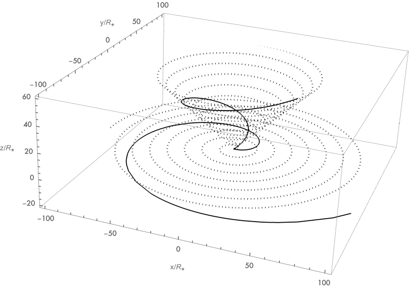
Figure 1: Magnetic field lines for $A=2$ (dotted curves) and $A=20$ (solid curves) for $\theta_{0}=\pi/4$ (conical surface) and $\theta_{0}=\pi/2$ (equatorial plane).

Figure 2 shows two field lines for $A=20$ (solid curves) for a value of $\theta_{0}=\pi/4$, and three lines of constant $p$ (dashed curves) on the same $\theta_{0}=\pi/4$ cone.

Figure 2: Magnetic field lines (solid curves) and lines of constant $p$ (dashed curves) for $A=20$ and $\theta_{0}=\pi/4$ (conical surface). The sphere at the center provides a point of reference and has radius $\xi=A=20.$

3 Magnetic Turbulence Structure

Guided by previous work (Giacalone & Jokipii, 1994; Casse et al., 2002; O’Sullivan et al., 2009; Fatuzzo et al., 2010; Fatuzzo & Adams, 2014), we develop a formalism for modeling Alfvénic MHD turbulence by using the orthogonal coordinate system developed in Section 2. At present, a complete theory of MHD turbulence in the interstellar medium remains elusive. Nevertheless, it is generally understood that turbulence is driven from a cascade of longer wavelengths to shorter wavelengths as a result of wave-wave interactions. For strong MHD turbulence in a uniform medium, this cascade seemingly produces eddies on small spatial scales that are elongated in the direction of the underlying magnetic field, so that the components of the wave vector $k_{\perp}$ and $k_{||}$ are related by the expression $k_{||}\propto k_{\perp}^{2/3}$ (Sridhar & Goldreich 1994; Goldreich & Sridhar 1995; Cho & Lazarian 2003). It is beyond the scope of this paper to extend these results for our non-uniform geometry. Since our aim here is to determine the possible effects of turbulence on cosmic ray propagation into a star/disk system, we will assume a reasonable form for the turbulent magnetic field as guided by basic principles.

Following the standard numerical approach for analyzing the fundamental physics of ionic motion in a turbulent magnetic field, we treat the total magnetic field ${\bf B}$ as a spatially turbulent component $\delta{\bf B}$ superimposed onto the static Parker spiral background field ${\bf B}_{P}$ described in Section 2. The turbulent field $\delta{\bf B}$ is generated by summing over a large number of randomly polarized waves with effective wave vectors $k_{n}$ logarithmically spaced between $k_{1}=k_{min}$ and $k_{N}=k_{max}$,

$$\delta{\bf B}=\sum_{n=1}^{N}\Lambda_{n}(p,q)\,\sin\left(k_{n}\,p+\beta_{n}\right)[\cos\alpha_{n}\hat{n}_{q}+\sin\alpha_{n}\hat{n}_{\theta}]\,,$$ (20)

where the direction and phase of each term is set through a random choice of $\alpha_{n}$ and $\beta_{n}$ (e.g., Giacalone & Jokipii 1994; Casse et al. 2002; O’Sullivan et al. 2009; Fatuzzo et al. 2010), and $\Lambda_{n}(p,q)$ is chosen to maintain the divergenceless condition (e.g., Equations 27 – 29) and to set the turbulence profile (e.g. Equation 30). Each term in the sum represents an Alfvénic wave in the sense that $\delta{\bf B}_{n}\perp{\bf B}_{P}$. Since the Alfvén speed $v_{A}$ is much less than that of the relativistic cosmic rays, we can adopt a static turbulent field (essentially a snapshot of the field configuration) for calculating the effects on particle motion. This simplification then removes the necessity of specifying a dispersion relation for each term. Although the discrete formalism adopted here represents an idealization of a continuous physical system, earlier works indicate that 25 terms per decade in $k$ space yields a robust description (e.g., Fatuzzo et al. 2016). We therefore take the number of terms in the sum of equation (20) to be $N=25\log_{10}(k_{max}/k_{min})$ throughout our work.

Since the variable $p$, which denotes the position along a field line, is undefined at $\xi=1$, an inner boundary for our analysis must be set arbitrarily. Toward that end, we combine equations (3) and (7) for $q=0$ to get the expression

$$p=A\ln\left(1-{1\over\xi}\right)+{\xi-1-\ln\xi\over A}\,,$$ (21)

which is then plotted in Figure 3 for $A=2$, 10, and 40 (solid curves), along with corresponding lines of the limiting form $p=\xi/A$ (dashed curves). We note that for $\xi\gtrsim A$, corresponding solid and dashed curves become nearly parallel, so the above expressions for $p$ are equivalent in our formalism. We therefore set the inner turbulence boundary for our system at $\xi_{t}=A$.

Figure 3: The solid curves denote the value of $p$ as a function of $\xi$ for a representative equatorial field line on which $q=0$ for $A$ = 2, 10, and 40. The dashed curves denote the corresponding values for the simple expression $p=\xi/A$.

To connect the wavevectors $k_{n}$ to their corresponding wavelengths $\lambda_{n}$, we first note that in the limit $\xi\gtrsim A$, $\Delta p\approx\Delta\phi\sin\theta_{0}$, which means that each term in the sum given by equation (20) represents a wave with $k_{n}\sin\theta_{0}$ wavelengths per winding of the background field. On the equatorial plane, this result can be couched in terms of the path length $s$ (in units of $R_{*}$) along a field line found by integrating the quantity

$$ds=\sqrt{d\xi^{2}+\xi^{2}d\phi^{2}}=\sqrt{{A^{2}+(\xi-1)^{2}\over A^{2}}}d\xi\,,$$ (22)

where the condition that $q$ remains constant on a field line has been used to relate $d\xi$ and $d\phi$. Integrating from the turbulence boundary (so that $s=p=0$ at $\xi=\xi_{t}=A$) then yields the expression

$$s={(\xi-1)\sqrt{A^{2}+(\xi-1)^{2}}-(A-1)\sqrt{A^{2}+(A-1)^{2}}\over 2A}+{A\over 2}\ln\left[{\xi-1+\sqrt{A^{2}+(\xi-1)^{2}}\over A-1+\sqrt{A^{2}+(A-1)^{2}}}\right]\,.$$ (23)

Coupled with equation (21), one then finds the approximate expression for the path length

$$s\approx{\xi^{2}-A^{2}\over 2A}\approx{Ap^{2}\over 2}\,,$$ (24)

which for $A=20$, yields a value of $p$ that is within $0.2$ of the true value for all s.

In Figure 4 we plot the sinusoidal dependence $\sin[kp]$ as a function of $s$ for an $A=20$ equatorial field line for cases where $k=1$ and $k=3$. The thin vertical lines denote locations where the field has wrapped around by 1, 2, 3, and 4 times, respectively (e.g, where $\phi$ has advanced by 2$\pi$, 4$\pi$, 6$\pi$, and 8$\pi$). As expected, one clearly sees that to a good approximation, there is one complete wavelength per winding for the $k=1$ mode, and three complete wavelengths per winding for the $k=3$ mode.

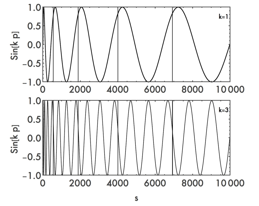
Figure 4: The function $\sin[kp]$ as a function of path length $s$ along a field line on the equatorial plane with $A=20$, for $k=1$ (upper panel) and $k=3$ (lower panel). The thin vertical lines at $s=548,1879,4001$, and $6913$ denote locations where the field line has wrapped around by 1, 2, 3, and 4 times, respectively (e.g, where $\phi$ has advanced by 2$\pi$, 4$\pi$, 6$\pi$, and 8$\pi$).

Although the wavelength of a given mode (as specified by $k_{n}$) increases with $s$, it is still useful to define an “effective wavelength” $\lambda_{n}(\xi)$ as equal to the displacement $\Delta s$ along an equatorial field line corresponding to $k_{n}\Delta p=2\pi$ (hence, $\lambda_{n}$ is also in units of $R_{*}$). Using equation (24), one finds

$$\lambda_{n}\equiv\Delta s\approx{A\over 2}\left[2p\Delta p+(\Delta p)^{2}\right]\approx\left[{2\pi\over k_{n}}\sqrt{\xi^{2}-A^{2}}+\lambda_{t;n}\right]\,,$$ (25)

where the effective wavelength at the turbulence boundary is given by

$$\lambda_{t;n}={2\pi^{2}A\over k_{n}^{2}}\,.$$ (26)

To complete the analysis, we ensure that the no-monopole condition $\nabla\cdot\delta{\bf B}_{n}=0$ is satisfied by selecting an appropriate form of the coefficients $\Lambda_{n}$. Toward that end, we use the divergence operator in our $(p,q,\theta)$ coordinate system to write the no-monopole condition as

$$\nabla\cdot\delta{\bf B}_{n}={\sin(k_{n}p+\beta_{n})\cos(\alpha_{n})\over h_{p}h_{q}h_{\theta}}\left[{\partial\over\partial q}(h_{p}h_{\theta}\Lambda_{n})\right]=0\,,$$ (27)

which requires

$$h_{p}h_{\theta}\Lambda_{n}=f(p)\;.$$ (28)

Using equations (10) and (12), and setting $f(p)$ equal to the constant $\Lambda_{t;n}$, one then finds

$$\Lambda_{n}(\xi)=\Lambda_{t;n}{A^{2}(A-1)\over\xi^{2}\,(\xi-1)}\ {\sqrt{A^{2}+(\xi-1)^{2}}\over\sqrt{A^{2}+(A-1)^{2}}}\;,$$ (29)

where the expression has been normalized so that $\Lambda_{n}(A)=\Lambda_{t;n}$. We note that $\Lambda_{n}\rightarrow\xi^{-2}$ when $\xi\gg A$, and in turn, $\delta B/B_{P}\rightarrow\xi^{-1}$.

The desired spectrum of the turbulent magnetic field is set through the appropriate choice of scaling for an assumed turbulent profile, i.e.,

$$\Lambda_{t;n}^{2}=\Lambda_{t;1}^{2}\left[{k_{n}\over k_{1}}\right]^{-\Gamma}{\Delta k_{n}\over\Delta k_{1}}=\Lambda_{t;1}^{2}\left[{k_{n}\over k_{1}}\right]^{-\Gamma+1}\,,$$ (30)

where $\Gamma=5/3$ is used for Kolmogorov turbulence. We note that for our logarithmic binning scheme, the value of $\Delta k_{n}/k_{n}$ is the same for all values of $n$. The value of $A_{t;1}$ is set by an amplitude parameter $\eta$ that specifies the average energy density of the turbulent field with respect to the background Parker-spiral field at the inner turbulence boundary; specifically, $\eta$ is defined through the expression

$$\eta={\langle\delta B^{2}\rangle\over B_{p;t}^{2}}\,,$$ (31)

where $B_{P;t}$ is the magnitude of the equatorial Parker spiral magnetic field at $\xi=A$ (our inner boundary for turbulence). In order to determine the entire structure of the magnetic field, we must specify the parameters $B_{*}$ (which then sets $B_{P;t}$), $A$, $k_{1}$, $k_{N}$, $\eta$, and $\Gamma$. We note, however, that since charged particle motion through a turbulent field is a resonant phenomena, the dynamics are not sensitive to the choice of $k_{N}$, so long as the particle radius of gyration falls within the range of largest and smallest fluctuations. Turbulent field lines are illustrated in Figure 5 for the case $A=20$, $k_{1}=1$, $k_{N}=10^{4}$ (so that $N=100$), $\eta=1$, and $\Gamma=5/3$.

Figure 5: Turbulent field lines for the case $A=20$, $k_{1}=1$, $k_{N}=10^{4}$, $\eta=1$, and $\Gamma=5/3$. The sphere at the center represents the turbulence boundary, and has radius $\xi=A=20.$

4 Particle Dynamics

The aim of this paper is to determine how cosmic-rays propagate through the magnetized disk environments surrounding T Tauri stars. We limit our analysis to relativistic protons, but note that our results are easily scaled to other cosmic-ray species. The general equations that govern the motion of protons with Lorentz factor $\gamma$ through a magnetic field take the well-know form

$${d{\bf u}\over dt}={c\over R_{0}}\,{{\bf u}\times{\bf b}\over\gamma}\qquad{\rm and}\qquad{d{\bf r}\over dt}=c{{\bf u}\over\gamma}\;,$$ (32)

where ${\bf u}=\gamma{\bf v}/c$, ${\bf b}={\bf B}/B_{*}$, and

$$R_{0}\equiv{m_{p}c^{2}\over eB_{*}}=3.1\times 10^{3}\,{\rm cm}\left({B_{*}\over 10^{3}\,\hbox{G}}\right)^{-1}\,.$$ (33)

The kinematics equations are readily solved given specified initial conditions (${\bf u_{i}}$ and ${\bf r_{i}}$) for our magnetic field geometry using standard numerical methods. For completeness, we note that the radius of gyration for a relativistic particle ($v\approx c$) moving through the spiral field at location $\xi$ with a pitch angle $\alpha_{p}$ is

$$R_{g}(\xi)={\gamma R_{0}B_{*}\sin\alpha_{p}\over B(\xi)}\,.$$ (34)

Cosmic-rays can only be funneled toward the T Tauri star if $R_{g}(\xi)/R_{*}\ll\xi$, which requires

$$\gamma\ll 4.8\times 10^{7}{\sqrt{A^{2}+(\xi-1)^{2}}\over A\xi}\left({B_{*}\over 10^{3}\,{\rm G}}\right)\,\left({R_{*}\over 1.5\times 10^{11}\,{\rm cm}}\right)\,$$ (35)

Important insight can be gleaned by considering the motion of particles in the limit $\xi\gg A$, for which ${\bf b}\approx(A\xi)^{-1}\hat{\phi}$. In this limit, the magnetic field has the same form as that of an infinite, straight, current-carrying wire. As shown in Aguierre et al. (2010), charged particles moving through such a field that have a radius of gyration smaller than their distance to the central wire will follow the field lines around the wire, but also exhibit a drift in the direction of the current. We extend the analysis for relativistic particles in Appendix B, and reach a similar conclusion. We do find, however, that the drift speed is proportional to the Lorentz factor $\gamma$ (see equation [B10]). These results are further confirmed numerically, as illustrated in Figure 6. In our analysis, we will therefore consider particles with a small enough Lorentz factor that their drift does not carry them a distance $R_{*}$ farther than the equatorial plane. Note that most of the ionization is expected to result from mildly relativistic particles: The cosmic ray flux increases rapidly with decreasing energy down to $E\sim 1$ GeV (Webber 1998; Moskalenko et al. 2002), and ionization is efficient for this energy range (see Umebayashi & Nakano 1981, Padovani et al. 2009, 2011; Cleeves et al. 2013). As a result, our results are expected to be robust.

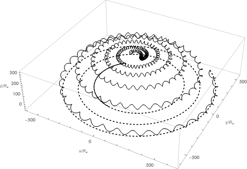
Figure 6: Trajectories for particles with Lorentz factors $\gamma=10^{5}$ (solid curve) and $\gamma=10^{3}$ (dashed curve) launched from the equatorial plane of a Parker spiral magnetic field with $A=20$ and adopted fiducial values of $B_{*}=10^{3}$ G and $R_{*}=1.5\times 10^{11}$ cm.

5 Effect of turbulence on cosmic-ray reflection

The magnetic moment of a relativistic proton

$$\mu={\gamma^{2}m_{p}\,v^{2}\sin^{2}\alpha_{p}\over 2B}\,,$$ (36)

is an adiabatic invariant under the condition that the field does not change significantly within a gyration radius, i.e., in the limit

$${\gamma}\ll{1\over R_{0}B_{*}}{B^{2}\over|\nabla B|}=4.8\times 10^{7}{\left[A^{2}+(\xi-1)^{2}\right]^{3/2}\over A\xi(2+2A^{2}-3\xi+\xi^{2})}\left({B_{*}\over 10^{3}\,{\rm G}}\right)\,\left({R_{*}\over 1.5\times 10^{11}\,{\rm cm}}\right)\,\,,$$ (37)

which similar to the condition expressed by equation (35). However, as is clear from Figure 6, a much stricter condition in our analysis is placed on the particle Lorentz factor by requiring that the particle drift is negligible in our numerical experiments.

Since the Lorentz factor of a particle remains constant in a time-independent magnetic field, the adiabatic invariance can be expressed as

$${\sin^{2}\alpha_{p}\over B}={\rm constant}\,.$$ (38)

As a charged cosmic-ray moves toward the star, its pitch angle must increase to match the increasing field strength. But since $\sin\alpha_{p}\leq 1$, the cosmic-ray must eventually be reflected at a mirror point where $\alpha_{p}=\pi/2$. To reach the turbulence boundary, a proton must therefore be injected from a radius $\xi_{i}$ with a pitch angle smaller than

$$\alpha_{crit}=\sin^{-1}\left[{A\left[A^{2}+(\xi_{i}-1)^{2}\right]^{1/4}\over\xi_{i}\left[A^{2}+(A-1)^{2}\right]^{1/4}}\right]\,.$$ (39)

For injected pitch angles $\alpha_{i}>\alpha_{crit}$, reflection occurs at a radius $\xi_{r}$ that can be well-approximated by solving the equation

$$\xi_{r}^{4}(A^{2}+\xi_{i}^{2})-\xi_{r}^{2}\xi_{i}^{4}\sin^{4}\alpha_{i}-A^{2}\xi_{i}^{4}\sin^{4}\alpha_{i}=0\,.$$ (40)

Figure 7 illustrates the location where reflection occurs as a function of injection pitch angle for particles injected from a radius $\xi_{i}=10^{4}$ on the equatorial plane of a (turbulence-free) Parker spiral field characterized by $A=2$ (solid curve), $A=20$ (dashed curve) and $A=40$ (dotted curve).

Figure 7: Reflection radius for $A=2$ (solid curve), $A=20$ (dashed curve), and $A=40$ (dotted curve) for a particle injected with pitch angle $\alpha_{i}$ at a radius $\xi_{i}=10^{4}$.

We investigate the effect of turbulence on reflection by running a suite of numerical experiments under different magnetic field scenarios. Each experiment is defined in terms of a specific magnetic profile (as set by the choice of $A$, $k_{1}$, $\Gamma$ and $\eta$), particle energetics (as defined by $\gamma$), and an injection scenario. The value of $k_{N}$ is set to ensure that the minimum wavelength is an order of magnitude smaller than the particle radius of gyration, both of which scale as $\xi$ (see discussion at the end of Section 3). We note from equation (25) that $\lambda_{min}\lesssim 2\pi\xi/k_{N}$ when $\xi\gtrsim A$, and from equations (6) and (34) that $R_{g}\approx\gamma AR_{0}\xi\sin\alpha$. We therefore set

$$k_{N}=10\left[{2\pi\xi R_{*}\over R_{g}}\right]={3\times 10^{9}\over\gamma A\sin\alpha_{crit}}\,\left({R_{*}\over 1.5\times 10^{11}\,{\rm cm}}\right)\,\left({B_{*}\over 10^{3}\,{\rm G}}\right)\,,$$ (41)

thereby invoking the smallest possible particle pitch angle. The value of $k_{1}$ is constrained by requiring that the longest effective boundary wavelength $\lambda_{t;1}$ be smaller than the radial extent of the T Tauriosphere, where, like our Heliosphere, the pressure from the stellar wind is balanced by ISM pressure. This boundary occurs at a radius that is on the order of 1000 AU (compared to $\sim 120$ AU for the Heliopause). Guided by equation (26), we thus invoke the constraint

$$k_{1}\geq k_{crit}\equiv\sqrt{{2\pi^{2}A\over 10^{5}}\left({R_{*}\over 1.5\times 10^{11}\,{\rm cm}}\right)}\,.$$ (42)

We adopt $k_{1}=10k_{crit}$ for most of our cases, but also consider larger and smaller values.

In addition to specifying the field structure, one must also specify the distribution of injected particles being considered. As noted above, most of the ionizing potential of cosmic-rays comes from moderately relativistic particles. However, the computational time required to complete the numerical experiments in our analysis for $\gamma\approx 1$ particles makes this choice of particle energies impractical. Luckily, the reflection point is not sensitive to the particle energy so long as particle drifting remains small, which then ensures that the conditions expressed in equations (35) and (37) are met. Taking everything into account, we adopt a Lorentz factor of $\gamma=10^{2}$.

Ideally, it makes sense to inject particles at the outer edge of the T-Taurisphere, which as noted above, occurs at a radius $\sim 1000$ AU. But given our choice of particle energy, the computational time required to integrate inward from the T-Taurisphere once again makes such a choice unfeasible. Since $\delta B\sim\xi^{-1}$, the effects of turbulence become increasingly significant as the particles gets closer to the star. We therefore arbitrarily set the injection boundary at 100 AU (which for $R_{*}=1.5\times 10^{11}$ cm, corresponds to $\xi_{i}=10^{4}$). As shown below, moving the injection boundary from 1,000 AU to 100 AU does not significantly affect the results, though care must be taken to properly interpret the injection distributions being considered.

The experiments performed and their corresponding output measures are listed in Table 1. Each experiment consists of numerically integrating the equations of motion for $N_{p}=300$ particles for a specified field structure (as defined by $A$, $\eta$, $k_{1}$, $\Gamma$), stellar parameters $R_{*}$ and $B_{*}$, and an injection scenario, but with each particle experiencing a different realization of the specified turbulent field as set through the random assignment of $\alpha_{n}$ and $\beta_{n}$ in equation (20). The mean and median of the ensuing distribution of reflection radii are then used as the output measures. Given the large number of system parameters, we consider only Kolmogorov turbulence ($\Gamma=5/3$), and adopt fiducial values of $B_{*}=10^{3}$ G and $R_{*}=1.5\times 10^{11}$ cm. We then explore how the parameters $\eta$, $A$, and $k_{min}$ affect particle reflection via experiments 1 - 7, for which all particles are injected at the critical angle (e.g. $\alpha_{i}=\alpha_{crit}$). Histograms of the resulting distributions of reflection radii are presented in Figure 8. In each panel, the mean of each distribution is represented by a vertical line (as defined in the figure caption), and can be compared directly to the known reflection radius in the absence of turbulence, which occurs at $\xi_{r}=A$.

Experiment 8 assess the overall effect that turbulence has on the ionization of a disk surrounding a T Tauri star. We assume the same turbulence profile as for Experiment 1, adopt a disk radius $R_{d}=50$ AU (e.g., $\xi_{d}=5,000$), and randomly pick the injection angle by selecting $\mu_{i}=\cos\alpha_{i}$ from a flat-top distribution ranging between $\cos\alpha_{R}$ and $\cos\alpha_{c}$ (where $\alpha_{R}=45^{o}$ is the injection pitch angle for which $\xi_{r}=\xi_{d}$ in a non-turbulent field). The histogram of the resulting distribution of reflection radii is presented in Figure 9, along with the corresponding distribution function in the absence of turbulence

$$f[\xi_{r}]=\left[{1\over\cos\theta_{c}-\cos\theta_{R}}\right]{d\mu\over d\xi_{r}}\,,$$ (43)

easily obtained from equation (40). The mean of the distribution for Exp. 8 (represented by the dashed vertical line in Figure 9) can be compared to its corresponding turbulent-free value

$$\langle\xi_{r}\rangle=\int_{A}^{\xi_{d}}\xi_{r}f[\xi_{r}]d\xi=2650\,.$$ (44)

Likewise, the median of the distribution (which appears in Table 1) can be compared to its corresponding turbulent-free value via the expression

$$\int_{A}^{\xi_{med}}f[\xi_{r}]d\xi=0.5\,,$$ (45)

which is easily calculated to be $\xi_{med}=2730$. While the mean and median values of Experiment 8 are quite similar to their non-turbulent counterparts, it is easily seen that turbulence does reduce the number of cosmic rays that reach the inner part ($\xi\lesssim 10^{3}$) of the disk. Of course, only a small fraction of cosmic-rays that enter the T-Taurisphere at 1000 AU (which for our choice of $R_{*}$ corresponds to $\xi=10^{5}$) will reach the disk. Specifically, for the physical conditions used in Experiment 8, particles would have to have a pitch angle of $\alpha_{T}\leq 12.9^{o}$ at the T-Taurisphere in order to reach the disk in the absence of turbulence. As such, the particles represented in Figure 10 account for only $f=1-\cos(12.9^{o})=0.025$ of all the particles that enter the T-Taurisphere for a Parker spiral with $A=20$.

		Summary	of	Experiments
Exp.	$\alpha_{i}$	$\eta$	$A$	$k_{1}$	$\langle\xi_{r}\rangle$	$\xi_{med}$
1	$\alpha_{c}$	1	20	$10k_{crit}$	105	97.4
2	$\alpha_{c}$	$0.1$	20	$10k_{crit}$	35.8	33.1
3	$\alpha_{c}$	$0.01$	20	$10k_{crit}$	28.8	30.1
4	$\alpha_{c}$	$1$	10	$10k_{crit}$	41.4	39.2
5	$\alpha_{c}$	$1$	40	$10k_{crit}$	210	198
6	$\alpha_{c}$	$1$	20	$k_{crit}$	67.3	54.3
7	$\alpha_{c}$	$1$	20	$100k_{crit}$	237	229
8	flat top	$1$	20	$10k_{crit}$	2640	2610

Table 1: Parameters are listed for each set of numerical experiments, including the pitch angle $\alpha_{i}$, the turbuence amplitude $\eta$, the magnetic field geometry parameter $A$, and the wavenumber $k_{1}$. The last two columns give the resulting values of the mean and median turning points of the distribution.

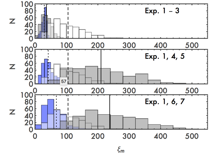
Figure 8: Distributions and corresponding means of reflection radii. Top panel - results for Exp. 1 (white histogram - dashed vertical line), Exp. 2 (gray histogram - solid vertical line) and Exp. 3 (blue histogram - dotted vertical line), for which the turbulence strength varies respectively from $\eta=1$, 0.1, and 0.01. Middle panel - results for Exp. 5 (gray histogram - solid vertical line), Exp. 1 (white histogram - dashed vertical line) and Exp. 4 (blue histogram - dotted vertical line), for which the magnetic profile parameter $A$ varies respectively from $A=40$, 20, and 10. Bottom panel - results for Exp. 7 (gray histogram - solid vertical line), Exp. 1 (white histogram - dashed vertical line) and Exp. 6 (blue histogram - dotted vertical line), for which the magnetic profile parameter $k_{min}$ varies respectively from $k_{min}=100k_{crit}$, $10k_{crit}$, and $k_{crit}$.

Figure 9: Distributions of reflection radii for Exp. 8. The vertical line denotes the mean of the distribution, and the solid curve represents the “normalized” distribution function $f_{r}[\xi_{r}]$ for a non-turbulent field.

To assess the impact of our choice of injection radius, we repeat Experiment 1, but inject particles at at radius of $\xi_{i}=2\times 10^{4}$ (200 AU). The ensuing distribution of pitch angles (with respect to the turbulent field) is then obtained at $\xi=10^{4}$ (100 AU), with the results shown in Figure 10. As expected, the presence of turbulence spreads out the distribution of pitch angles about the non-turbulence field value (depicted by the vertical line). Not surprisingly, this spread is quite narrow owing to the fact that the turbulent field scales as $\delta B\sim\xi^{-1}$. If these particles continued spiraling inward in a non-turbulent field, the corresponding distribution of reflection radii $\xi_{r}$ would range between 17 and 25, which is much narrower than the distribution of reflection radii obtained in Experiment 1. As such, the distributions obtained in our experiments, for which particle injection occurred at $\xi_{i}=10^{4}$, would be very similar to those that would have been obtained had we injected the particles at $\xi=10^{5}$.

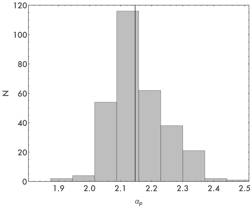
Figure 10: Distributions of pitch angles resulting at $\xi=100$ for particles injected at $\xi_{i}=200$, all with a critical pitch angle, into a turbulent magnetic field with the same profile as used in Experiment 1. The vertical line represents the value of the pitch angle that particles would have in the absence of turbulence.

We conclude our analysis by considering the effectiveness of cosmic-rays propagating inward from the T-Taurisphere at ionizing a circumstellar disk. Toward that end, we adopt the following fiducial values of the system parameters (e.g., Hartmann 2009): disk radius $R_{d}=50$ AU, disk mass $M_{d}=0.05M_{*}$, and stellar mass $M_{*}=M_{\odot}$. We also adopt standard temperature, density, and surface density profiles of the form

$$T(r)=T_{d}\left({R_{d}\over r}\right)^{1/2}\,,\qquad\rho(r,z)=\rho(r)e^{-{z^{2}/H^{2}}}\,\qquad{\rm and}\qquad\Sigma(r)=\Sigma_{c}\left({R_{d}\over r}\right)^{p}\,.$$ (46)

In this treatment, the scale height $H(r)$ is taken to be the product of the sound speed $a_{s}=\sqrt{kT/(2m_{p})}$ and rotation rate $\Omega(r)=\sqrt{GM_{*}/r^{3}}$. The temperature and surface density scales are $T_{d}=30$ K and $\Sigma_{c}=14$ g cm^-2, respectively, and the power-law index of the surface density is set at $p=3/2$. With these choices, the expression for the mid-plane density becomes

$$\rho_{m}(r)=1.3\times 10^{-13}\,{\rm g}\,{\rm cm}^{-3}\,\left({R_{d}\over r}\right)^{11/4}\,.$$ (47)

Since protons are attenuated exponentially with a characteristic length of $\Sigma_{0}=69$ g cm^-2 (Umebayashi & Nakano 1981), cosmic-rays entering the outer edge of the disk would lose their ionizing potential after traveling a distance $L\sim\Sigma_{0}/\rho(R_{d})\sim 35$ AU - which for a spiral path, occurs within the first inward spiral. Disk ionization is thus expected to result primarily from particles coming inward near the equatorial plane, but moving a few scale-heights above, where the density is significantly lower than at the mid-plane. We note, however, that at large column densities, the ionization rate is not due to protons, but to secondary particles (electrons and positrons) produced by charged and neutral pion decay through proton-proton collisions. The attenuation column for ionization is $115$ g cm^-2 between 100 and 500 g cm^-2 from the surface, whereas the ionization attenuation length is 96 g cm^-2 above 500 g cm^-2 (Umebayashi & Nakano 1981). In any case, although our analysis was performed for particles moving along the equatorial mid-plane, the field structure within the disk will be fairly uniform, and our results then applicable throughout the disk. We are therefore able to construct a working estimate for the effects of magnetic turbulence on the inward propagation of cosmic rays from the T-Tauiosphere inward to the circumstellar disk. Nonetheless, a detailed analysis of the overall ionization structure within T-Tauri disks is left for future work. A host of additional effects should be considered, including ion-neutral damping and its back-reaction on the regions of the disk where turbulence can be active (see the discussion of Section 6.2).

6 Conclusion

Cosmic rays represent an important source of ionization for the disks associated with young stars. These disk environments provide the sites for planet formation and the ionization levels affect the process. This paper considers the propagation of cosmic rays through spiral magnetic fields, such as those produced by stellar winds, with a focus on the parameter space applicable to T Tauri star/disk systems. In this treatment, turbulent fluctuations to the magnetic field are included, and their effects on the inward propagation of cosmic rays are determined. Our specific results are summarized below (Section 6.1) along with a discussion of their implications (Section 6.2).

6.1 Summary of Results

In order to study the propagation of cosmic rays through turbulent magnetic fields, we first construct a new coordinate system where one of the coordinates follows the unperturbed magnetic field lines (Section 2). The unperturbed field is assumed to follow a Parker spiral. We then construct the perpendicular coordinates and the necessary differential operators. Note that T Tauri stars rotate faster than the Sun, so that the winding parameters fall in a different regime than for the Solar case. The new coordinate system allows us to construct Alfvénic field fluctuations (Section 3), where the perturbations are perpendicular to the original field lines and where the fluctuations manifestly have zero divergence.

With the magnetic field structure and turbulent fluctuations specified, we have carried out a large ensemble of numerical integrations to follow the inward propagation of cosmic rays (Section 5). The system is characterized by a number of parameters, including the winding parameter of the original spiral structure $A=v_{w}/v_{rot}$, the amplitude of the turbulent fluctuations $\eta$, the minimum wave number $k_{1}$, the spectral index of the turbulent cascade $\Gamma$, the magnetic field strength of the stellar surface $B_{\ast}$, the initial pitch angles $\alpha_{i}$, and the cosmic ray energies as determined by the Lorentz factor $\gamma$. In addition, due to the stochastic nature of the turbulence, each cosmic ray will experience a different realization of the magnetic field fluctuations as it propagates inward.

The results of our numerical experiments are presented in Figures 8 – 10 for different choices of the aforementioned system parameters. In the absence of turbulence, incoming cosmic rays with a given set of initial conditions $(\alpha,\gamma)$ would reach a well-defined inner turning point that represents an inner boundary to their sphere of influence. The inclusion of turbulence replaces this well-defined mirror point with a distribution of values. The width of this distribution increases with the amplitude of the turbulent fluctuations. In addition, for small amplitudes $\eta\ll 1$, these distributions can be modeled as Gaussians, where the turning point for the non-turbulent fields lies at the center of the distribution. For larger fluctuation amplitudes, however, the distributions become highly non-gaussian, and the mean of the distribution falls outside the turning point of the unperturbed system. As a result, the presence of turbulence acts to significantly reduce the flux of cosmic rays that enter the inner parts of disks. The reduction becomes significant, with the mean turning point radius becoming twice as large, when the turbulent amplitude $\eta\lower 2.15277pt\hbox{$\;\buildrel>\over{\sim}\;$}0.3$.

6.2 Discussion

This paper has presented an semi-analytic treatment of cosmic ray propagation through the turbulent magnetic fields expected in the environments associated with young star/disk systems. As outlined above, this work elucidates the basic physics of cosmic ray transport and shows that turbulence acts to suppress the cosmic ray flux and hence the ionization rate. Although this subject is well developed for the Solar Wind (e.g., see the reviews of Goldstein et al. 1995; Tu & Marsch 1995), relatively little work has been done for young stars. The necessity for understanding cosmic ray ionization rates was emphasized by Gammie (1996), who showed that cosmic rays cannot penetrate to the mid-plane of circumstellar disks, so that dead zones with little ionization develop. Additional suppression of the external cosmic ray flux through the action of T Tauri winds was considered by Cleeves et al. (2013), who introduced the concept of a T Tauriosphere, a region surrounding the star/disk system with suppressed cosmic ray flux. This paper studies the propagation of cosmic rays inward from the T Tauriopause, toward the inner disk regions that are susceptible to dead zones, and thus acts to connect these previous calculations. Nonetheless, many avenues for additional work should be pursued.

This work focuses on the case where the unperturbed fields follow a spiral form (as in Parker 1958). However, alternate — and more complicated — field geometries should be explored. In addition, the parameter space available for these star/disk/magnetic systems is quite large and a full exploration of the entire $(A,\alpha_{i},k_{1},\Gamma,B_{\ast},\gamma)$ space is beyond the scope of any single contribution. This work uses a simple prescription for the turbulence, but more sophisticated treatments should be employed. Finally, this work proceeds using semi-analytic methods. Since much of the previous literature for circumstellar disks simply uses the standard (single) value of the interstellar cosmic rate ionization rate ($\zeta\sim 10^{-17}$ s^-1, Umebayashi & Nakano 1981), this work provides an important step forward. Nonetheless, full MHD simulations of the problem should also be carried out. These numerical treatments can include additional effects beyond what is possible with a semi-analytic approach. For example, we have assumed that the turbulence remains active throughout the region of cosmic ray propagation. However, this assumption could be modified by ion-neutral damping, which reduces the amplitude of magnetic turbulence when the frequency of magnetic waves is comparable to the frequency of ion–neutral collisions. With effective damping, the turbulence levels could have spatial dependence that is not addressed herein.

The results of this work inform a number of applications. Turbulence in the disk itself is thought to provide one source for disk viscosity, which is necessary for disk accretion to occur. The disk turbulence is (most likely) driven by MHD instabilities such as MRI Balbus & Hawley (1991), which requires ionization levels high enough to couple the gas to the magnetic field. Cosmic rays provide an important source of ionization, especially in the outer regions of the disk (beyond $\sim 10$ AU). This paper shows that the flux of cosmic rays can be suppressed as the particles propagate inward from the Tauriopause to the disk itself. This reduced cosmic ray flux will, in turn, reduce the regions of the disk that is sufficiently ionized for the MRI to be active. An important topic for the future is to build models that study cosmic ray propagation inward through both stellar winds and magnetic turbulence. The stellar winds suppress the cosmic ray flux within their sphere of influence — the T Tauriosphere — which specifies the inner boundary condition for the continued inward propagation of cosmic rays as considered in this paper. The mirroring effects, enhanced by turbulence, then provide additional suppression of the flux. A combined treatment should thus study how the cosmic ray flux in jointly modulated by the action of both stellar winds and turbulent magnetic fields.

Appendix A Construction of Orthogonal Coordinates

In this Appendix, we show how the co-ordinate $p(\xi,\phi)$ can be obtained from the co-ordinate $q$ using the conditions that these co-ordinates are orthogonal. For simplicity, we adopt a dimensionless spherical co-ordinate system ($\xi,\theta,\phi$). Starting with the definition

$$q\equiv\xi-1-\ln{\xi}-A\phi\sin\theta_{0}\,,$$ (A1)

we now look for a co-ordinate $p$ such that $\nabla p\perp\nabla q$. Since

$$\nabla q={\xi-1\over\xi}\hat{\xi}-{A\sin\theta_{0}\over\xi\sin\theta}\hat{\phi}\,,$$ (A2)

this condition is met so long as

$$\nabla p=\left[{A\sin\theta_{0}\over\sin\theta}\hat{\xi}+\left(\xi-1\right)\hat{\phi}\right]\,f(\xi,\theta,\phi)\,,$$ (A3)

which in turn requires

$${\partial p\over\partial\xi}={A\sin\theta_{0}\over\sin\theta}f(\xi,\theta,\phi)\,,$$ (A4)

and

$${\partial p\over\partial\phi}=\xi(\xi-1)\sin\theta f(\xi,\theta,\phi)\,.$$ (A5)

Combining these conditions, one finds that $f(\xi,\theta,\phi)$ must satisfy the equation

$${A\sin\theta_{0}\over\sin\theta}{\partial f\over\partial\phi}=\left(2\xi-1\right)\sin\theta f+\xi\left(\xi-1\right)\sin\theta{\partial f\over\partial\xi}\,.$$ (A6)

Here we use separation of variables and constrain our solutions to lie on the surface given by $\theta=\theta_{0}$, and thus look for solutions of the form

$$f(\xi,\phi)=\Xi[\xi]\,\Phi[\phi]\,,$$ (A7)

which yields the equation

$${A\over\sin\theta_{0}}{1\over\Phi}{d\Phi\over d\phi}=(2\xi-1)+\xi(\xi-1){1\over\Xi}{d\Xi\over d\xi}\,.$$ (A8)

Upon substitution of the trivial solution

$$\Phi=e^{m\phi}\,$$ (A9)

one then is left to solve the equation

$${d\Xi\over\Xi}=\left[{mA\over\sin\theta_{0}}-(2\xi-1)\right]\,{d\xi\over\xi(\xi-1)}\,.$$ (A10)

Integrating this equation then yields

$$\ln\Xi=(mA^{\prime}-1)\ln(\xi-1)-(mA^{\prime}+1)\ln\xi\,,$$ (A11)

where $A^{\prime}\equiv A/\sin\theta_{0}$. In turn

$$f(\xi,\phi)=\left[{(\xi-1)^{mA^{\prime}-1}\over\xi^{mA^{\prime}+1}}\right]e^{m\phi}\,,$$ (A12)

and subsequently,

$$p(\xi,\phi)=\left[{(\xi-1)^{mA^{\prime}}\over\xi^{mA^{\prime}}}\right]{e^{m\phi}\over m}\,.$$ (A13)

The exponential dependence on $\phi$ in equation (A13) does not seem physical. We note, however, that in the limit $m\rightarrow 0$, $f\rightarrow\xi^{-1}(\xi-1)^{-1}$. Equation (A4) can then be integrated to yield

$$p=A\log\left({\xi-1\over\xi}\right)\,,$$ (A14)

and equation (A5) can be integrated to yield

$$p=\phi\sin\theta_{0}\,.$$ (A15)

Adding these solutions then yields the expression adopted in our work:

$$p=A\ln\left(1-{1\over\xi}\right)+\phi\sin\theta_{0}\,.$$ (A16)

Appendix B Drift for Relativistic Particles

Following the analysis of Aguirre et al. (2010), we write the particle velocity and acceleration in cylindrical co-ordinates in dimensionless form:

$${\vec{\beta}}=\dot{\bar{r}}\hat{r}+\bar{r}\dot{\phi}\hat{\phi}+\dot{\bar{z}}\hat{z}\,,$$ (B1)

and

$$\dot{\vec{\beta}}=(\ddot{\bar{r}}-\bar{r}\dot{\phi}^{2})\hat{r}+(\bar{r}\ddot{\phi}+2\dot{\bar{r}}\dot{\phi})\hat{\phi}+\ddot{\bar{z}}\hat{z}\,,$$ (B2)

and rewrite equation (32) as

$$(\ddot{\bar{r}}-\bar{r}\dot{\phi}^{2})=-{\dot{\bar{z}}R_{*}\over\gamma AR_{0}\bar{r}}\qquad\qquad(\bar{r}\ddot{\phi}+2\dot{\bar{r}}\dot{\phi})=0\qquad\qquad\ddot{\bar{z}}={\dot{\bar{r}}R_{*}\over\gamma AR_{0}\bar{r}}\,.$$ (B3)

The second and third equations can be integrated to yield constants of the motion:

$$L=\bar{r}^{2}\dot{\phi}\,,$$ (B4)

and

$$P=\dot{\bar{z}}-{R_{*}\over A\gamma R_{0}}\ln\bar{r}\,.$$ (B5)

Without loss of generality, we can set an initial condition for a particle with Lorentz factor $\gamma$ at $\bar{r}=\bar{r}_{i}$ with $\dot{\bar{z}}_{i}=0$, where $\bar{r}_{i}$ effectively replaces the constant $P$ in equation (B5):

$$\dot{\bar{z}}={R_{*}\over A\gamma R_{0}}\ln\left[{\bar{r}\over\bar{r}_{i}}\right]\,,$$ (B6)

Integration then yields

$$\bar{z}(\bar{t})=\bar{z}_{0}+{R_{*}\over A\gamma R_{0}}\int_{0}^{\bar{t}}\ln\left[{\bar{r}(\bar{t}^{\prime})\over\bar{r}_{i}}\right]d\bar{t}^{\prime}\,.$$ (B7)

Since $r_{i}$ is a periodic function with some periodicity $T_{0}$, the integral can be written as

$$\int_{0}^{\bar{t}}\ln\left[{\bar{r}(\bar{t}^{\prime})\over\bar{r}_{i}}\right]d\bar{t}^{\prime}={\bar{t}\over T_{0}}\int_{0}^{T_{0}}\ln\left[{\bar{r}(\bar{t}^{\prime})\over\bar{r}_{i}}\right]d\bar{t}^{\prime}+G(\bar{t})\,,$$ (B8)

where $G(\bar{t})$ is a function with periodicity $T_{0}$. Using equation (B3), one then obtains

$$\bar{z}(\bar{t})=\bar{z}_{0}+{\bar{t}\over T_{0}}{A\gamma R_{0}\over R_{*}}\,\int_{t_{-}}^{t_{+}}\left[{L^{2}\over\bar{r}^{2}}+\dot{\bar{r}}^{2}\right]d\bar{t}^{\prime}+{R_{*}\over A\gamma R_{0}}G(\bar{t})\,,$$ (B9)

where $t_{-}$ and $t_{+}$ are the time values where $\bar{r}(\bar{t})$ reaches its minimum and maximum values, and $L={\bar{r}_{i}}^{2}\dot{\phi}_{i}$. The particle therefore drifts in the $z$ direction with a (dimensionless) drift speed

$$v_{drift}={A\gamma R_{0}\over T_{0}R_{*}}\,\int_{t_{-}}^{t_{+}}\left[{L^{2}\over\bar{r}^{2}}+\dot{\bar{r}}^{2}\right]d\bar{t}^{\prime}\,,$$ (B10)

which is proportional to the Lorentz factor $\gamma$.

References

- \appedix
- Adams (2011) Adams, F. C. 2011, ApJ, 730, 27
- Adams & Gregory (2012) Adams, F. C., & Gregory, S. G. 2012, ApJ, 744, 55
- Aguierr & Gregory (2010) Aguirre, J., Luque, A., & Peralta-Salas, D. 2010, Physica D, 239, 654
- Balbus & Hawley (1991) Balbus, S. A., & Hawley, J. F. 1991, ApJ, 376, 214
- Casse et al. (2002) Casse, F., Lemoine, M., & Pelletier, G. 2002, Phys. Rev. D, 65, 023002
- Chapman et al. (2013) Chapman, N. L., et al. 2013, ApJ, 770, 151
- Cho & Lazarian (2003) Cho, J., & Lazarian, A. 2003, MNRAS, 345, 325
- Cleeves et al. (2013) Cleeves, L. I., Adams, F. C., & Bergin. E. A. 2013, ApJ, 772, 5
- Cleeves et al. (2015) Cleeves, L. I., Bergin, E. A., Qi, C., Adams, F. C., & Öberg, K. I. 2015, ApJ, 799, 204
- Davidson et al. (2011) Davidson, J. A., Novak, G., Matthews, T. G., Matthews, B., Goldsmith, P. F., Chapman, N., Volgenau, N. H., Vaillancourt, J. E., & Attard, M. 2011, ApJ, 732, 97
- Desch et al. (2004) Desch, S. J., Connolly, H. C., Jr., & Srinivasan, G. 2004, ApJ, 602, 528
- Fatuzzo et al. (2010) Fatuzzo, M., Melia, F., Todd, E., & Adams, F. C. 2010, ApJ, 725, 515
- Fatuzzo & Adams (2014) Fatuzzo, M., & Adams, F. C. 2014, ApJ, 787, 26
- Fatuzzo et al. (2016) Fatuzzo, M., Holden, L, Grayson, L. & Wallace, K. 2016, PASP, 128, 968
- Galli & Shu (1993) Galli, D. & Shu, F. H. 1993, ApJ, 417, 220
- Gammie (1996) Gammie, C. F. 1996, ApJ, 457, 355
- Giacalone & Jokipii (1994) Giacalone, J. & Jokipii, J. R. 1994, ApJL, 430, L137
- Glassgold & Langer (1973) Glassgold, A. E., & Langer, W. D. 1973, ApJ, 186, 859
- Goldreich & Sridhar (1995) Goldreich, P., & Sridhar, S. 1995, ApJ, 438, 763
- Goldstein et al. (1995) Goldstein, M. L., Roberts, D. A., & Matthaeus, W. H. 1995, ARA&A, 33, 283
- Hartmann (2009) Hartmann, L. W. 2009 Accretion Processes in Star Formation: Second Edition, (Cambridge: Cambridge Univ. Press)
- Hayakawa et al. (1961) Hayakawa, S., Nishimura, S., & Takayanagi, T. 1961, PASJ, 13, 184
- Maclow & Klessen (2004) Mac-Low, M.-M. & Klessen, R. S. 2004, Review of Modern Physics, 76, 125
- Moskalenko et al. (2002) Moskalenko, I. V., Strong, A. W., Ormes, J. F., & Potgieter, M. S. 2002, ApJ, 565, 280
- Ostriker et al. (2001) Ostriker, E. C., Stone, J. M., & Gammie, C. F. 2001, ApJ, 546, 980
- O’Sullivan et al. (2009) O’Sullivan, S., Reville, B., & Taylor, A. M. 2009, MNRAS, 400, 248
- Padoan et al. (2001) Padoan, P.,Goodman, A., Draine, B. T., Juvela, M., Nordlund, A., & Rögnvaldsson, O. E. 2001, ApJ, 559, 1005
- Padoan & Scalo (2005) Padoan, P., & Scalo, J. 2005, ApJ, 624, L97
- Padovani et al. (2009) Padovani, M., Galli, D., & Glassgold, A. E. 2009, A&A, 501, 619
- Padovani & Galli (2011) Padovani, M., & Galli, D. 2011, A&A, 530, 109
- Padovani et al. (2013) Padovani, M., Hennebelle, P., & Galli, D. 2013, A&A, 560, 114
- Parker (1958) Parker, E. N. 1958, Phys. Rev., 110, 1445
- Qiu et al. (2014) Qiu, K., Zhang, Q., Menten, K. M., Liu, H. B., Tang, Y.-W., Girart, J. M. 2014, ApJ, 794, L18
- Semenov et al. (2004) Semenov, D., Wiebe, D., & Henning, T. 2004, A&A, 417, 93
- Shu et al. (1987) Shu, F. H., Adams, F. C., & Lizano, S. 1987, ARA&A, 25, 23
- Spitzer & Tomasko (1968) Spitzer, L., & Tomasko, M. G. 1968, ApJ, 152, 971
- Sridhar & Goldreich (1994) Sridhar, S., & Goldreich, P. 1994, ApJ, 432, 612
- Tu & Marsch (1995) C.-Y. Tu & E. Marsch, 1995, Space Sci. Rev., 73, 1
- Umebayashi & Nakano (1981) Umebayashi, T., & Nakano, T. 1981, PASJ, 33, 617
- Webber (1998) Webber, W. R. 1998, ApJ, 506, 329
- Weinreich (1998) Weinreich, G. 1998, Geometrical Vectors (Chicago: Univ. Chicago Press)