Convergence rates for distributed stochastic optimization over random networks

Abstract

We establish the $O(\frac{1}{k})$ convergence rate for distributed stochastic gradient methods that operate over strongly convex costs and random networks. The considered class of methods is standard – each node performs a weighted average of its own and its neighbors’ solution estimates (consensus), and takes a negative step with respect to a noisy version of its local function’s gradient (innovation). The underlying communication network is modeled through a sequence of temporally independent identically distributed (i.i.d.) Laplacian matrices connected on average, while the local gradient noises are also i.i.d. in time, have finite second moment, and possibly unbounded support. We show that, after a careful setting of the consensus and innovations potentials (weights), the distributed stochastic gradient method achieves a (order-optimal) $O(\frac{1}{k})$ convergence rate in the mean square distance from the solution. This is the first order-optimal convergence rate result on distributed strongly convex stochastic optimization when the network is random and/or the gradient noises have unbounded support. Simulation examples confirm the theoretical findings.

1 Introduction

Distributed optimization and learning algorithms attract a great interest in recent years, thanks to their widespread applications including distributed estimation in networked systems, e.g., [1], distributed control, e.g., [2], and big data analytics, e.g., [3].

In this paper, we study distributed stochastic optimization algorithms that operate over random networks and minimize smooth strongly convex costs. We consider standard distributed stochastic gradient methods where at each time step, each node makes a weighted average of its own and its neighbors’ solution estimates, and performs a step in the negative direction of its noisy local gradient. The underlying network is allowed to be randomly varying, similarly to, e.g., the models in [4, 5, 6]. More specifically, the network is modeled through a sequence of independent identically distributed (i.i.d.) graph Laplacian matrices, where the network is assumed to be connected on average. (This translates into the requirement that the algebraic connectivity of the mean Laplacian matrix is strictly positive.) Random network models are highly relevant in, e.g., internet of things (IoT) and cyber physical systems (CPS) applications, like, e.g., predictive maintenance and monitoring in industrial manufacturing systems, monitoring smart buildings, etc. Therein, networked nodes often communicate through unreliable/intermittent wireless links, due to, e.g., low-power transmissions or harsh environments.

The main contributions of the paper are as follows. We show that, by carefully designing the consensus and the gradient weights (potentials), the considered distributed stochastic gradient algorithm achieves the order-optimal $O(1/k)$ rate of decay of the mean squared distance from the solution (mean squared error – MSE). This is achieved for twice continuously differentiable strongly convex local costs, assuming also that the noisy gradients are unbiased estimates of the true gradients and that the noise in gradients has bounded second moment. To the best of our knowledge, this is the first time an order-optimal convergence rate for distributed strongly convex stochastic optimization has been established for random networks.

We now briefly review the literature to help us contrast this paper from prior work. In the context of the extensive literature on distributed optimization, the most relevant to our work are the references on: 1) distributed strongly convex stochastic (sub)gradient methods; and 2) distributed (sub)gradient methods over random networks (both deterministic and stochastic methods). For the former thread of works, several papers give explicit convergence rates under different assumptions. Regarding the underlying network, references [7, 8] consider static networks, while the works [9, 10, 11] consider deterministic time-varying networks.

References [7, 8] consider distributed strongly convex optimization for static networks, assuming that the data distributions that underlie each node’s local cost function are equal (reference [7] considers empirical risks while reference [8] considers risk functions in the form of expectation); this essentially corresponds to each nodes’ local function having the same minimizer. References [9, 10, 11] consider deterministically varying networks, assuming that the “union graph” over finite windows of iterations is connected. The papers [7, 8, 9, 10] assume undirected networks, while [11] allows for directed networks but assumes a bounded support for the gradient noise. The works [7, 9, 10, 11] allow the local costs to be non-smooth, while [8] assumes smooth costs, as we do here. With respect to these works, we consider random networks, undirected networks, smooth costs, and allow the noise to have unbounded support.

Distributed optimization over random networks has been studied in [4, 5, 6]. References [4, 5] consider non-differentiable convex costs and no (sub)gradient noise, while reference [6] considers differentiable costs with Lipschitz continuous and bounded gradients, and it also does not allow for gradient noise, i.e., it considers methods with exact (deterministic) gradients. In [12], we consider a distributed Kiefer-Wolfowitz-type stochastic approximation method and establish the method’s $O(1/k^{1/2})$ convergence rate. Reference [12] complements the current paper by assuming that nodes only have access to noisy functions’ estimates (zeroth order optimization), and no gradient estimates are available. In contrast, by assuming a noisy first-order (gradient) information is available, we show here that strictly faster rates than in [12] can be achieved.

In summary, to the best of our knowledge, this is the first time to establish an order-optimal convergence rate for distributed stochastic gradient methods under strongly convex costs and random networks.

Paper organization. The next paragraph introduces notation. Section 2 describes the model and the stochastic gradient method we consider. Section 3 states and proves the main result on the algorithm’s MSE convergence rate. Section 4 provides a simulation example. Finally, we conclude in Section 5.

Notation. We denote by $\mathbb{R}$ the set of real numbers and by ${\mathbb{R}}^{m}$ the $m$-dimensional Euclidean real coordinate space. We use normal lower-case letters for scalars, lower case boldface letters for vectors, and upper case boldface letters for matrices. Further, we denote by: $\mathbf{A}_{ij}$ the entry in the $i$-th row and $j$-th column of a matrix $\mathbf{A}$; $\mathbf{A}^{\top}$ the transpose of a matrix $\mathbf{A}$; $\otimes$ the Kronecker product of matrices; $\mathbf{I}$, $0$, and $\mathbf{1}$, respectively, the identity matrix, the zero matrix, and the column vector with unit entries; $\mathbf{J}$ the $N\times N$ matrix $J:=(1/N)\mathbf{1}\mathbf{1}^{\top}$. When necessary, we indicate the matrix or vector dimension through a subscript. Next, $A\succ 0\,(A\succeq 0)$ means that the symmetric matrix $A$ is positive definite (respectively, positive semi-definite). We further denote by: $\|\cdot\|=\|\cdot\|_{2}$ the Euclidean (respectively, spectral) norm of its vector (respectively, matrix) argument; $\lambda_{i}(\cdot)$ the $i$-th smallest eigenvalue; $\nabla h(w)$ and $\nabla^{2}h(w)$ the gradient and Hessian, respectively, evaluated at $w$ of a function $h:{\mathbb{R}}^{m}\rightarrow{\mathbb{R}}$, $m\geq 1$; $\mathbb{P}(\mathcal{A})$ and $\mathbb{E}[u]$ the probability of an event $\mathcal{A}$ and expectation of a random variable $u$, respectively. Finally, for two positive sequences $\eta_{n}$ and $\chi_{n}$, we have: $\eta_{n}=O(\chi_{n})$ if $\limsup_{n\rightarrow\infty}\frac{\eta_{n}}{\chi_{n}}<\infty$.

2 Model and algorithm

2-A Optimization and network models

We consider the scenario where $N$ networked nodes aim to collaboratively solve the following unconstrained problem:

$$\mathrm{minimize\,\,\,\,}\sum_{i=1}^{N}f_{i}(\mathbf{x}),$$ (1)

where $f_{i}:\mathbb{R}^{m}\mapsto\mathbb{R}$ is a convex function available to node $i$, $i=1,...,N$. We make the following standard assumption on the $f_{i}$’s.

Assumption 1.

For all $i=1,...,N$, function $f_{i}:\mathbb{R}^{m}\mapsto\mathbb{R}$ is twice continuously differentiable, and there exist constants $0<\mu\leq L<\infty$, such that, for all $\mathbf{x}\in{\mathbb{R}}^{m}$, there holds:

$$\mu\,\mathbf{I}\preceq\nabla^{2}f_{i}(\mathbf{x})\preceq L\,\mathbf{I}.$$

Assumption 1 implies that each $f_{i}$ is strongly convex with modulus $\mu$, and it also has Lipschitz continuous gradient with Lipschitz constant $L$, i.e., the following two inequalities hold for any $\mathbf{x,y}\in{\mathbb{R}}^{m}$:

$$f_{i}(\mathbf{y})\geq f_{i}(\mathbf{x})+\nabla f_{i}(\mathbf{x})^{\top}\,(\mathbf{y}-\mathbf{x})+\frac{\mu}{2}\|\mathbf{x}-\mathbf{y}\|^{2}$$

$$\|\nabla f_{i}(\mathbf{x})-\nabla f_{i}(\mathbf{y})\|\leq L\,\|\mathbf{x}-\mathbf{y}\|.$$

Furthermore, under Assumption 1, problem (1) is solvable and has the unique solution, which we denote by $x^{\star}\in{\mathbb{R}}^{m}$. For future reference, introduce also the sum function $f:\,{\mathbb{R}}^{m}\rightarrow\mathbb{R}$, $f(\mathbf{x})=\sum_{i=1}^{N}f_{i}(\mathbf{x})$.

We consider distributed stochastic gradient methods to solve (1) over random networks. Specifically, we adopt the following model. At each time instant $k=0,1,...$, the underlying network $\mathcal{G}(k)=(V,\mathbf{E}(k))$ is undirected and random, with $V=\{1,...,N\}$ the set of nodes, and $\mathbf{E}(k)$ the random set of undirected edges. We denote by $\{i,j\}$ the edge that connects nodes $i$ and $j$. Further, denote by 7 $\Omega_{i}(k)=\{j\in V:\,\,\{i,j\}\in\mathbf{E}(k)\}$ the random neighborhood od node $i$ at time $k$ (excluding node $i$). We associate to $\mathcal{G}(k)$ its $N\times N$ (symmetric) Laplacian matrix $\boldsymbol{\mathcal{L}}(k)$, defined by: $\boldsymbol{\mathcal{L}}_{ij}(k)=-1,$ if $\{i,j\}\in\mathbf{E}(k)$, $i\neq j$; $\boldsymbol{\mathcal{L}}_{ij}(k)=0,$ if $\{i,j\}\notin\mathbf{E}(k)$, $i\neq j$; and $\boldsymbol{\mathcal{L}}_{ii}(k)=-\sum_{j\neq i}\boldsymbol{\mathcal{L}}_{ij}(k).$ Denote by $\overline{\boldsymbol{\mathcal{L}}}=\mathbb{E}[\,\boldsymbol{\mathcal{L}}(k)\,]$ (as explained ahead, the expectation is independent of $k$), and let $\overline{\mathcal{G}}=(V,\overline{\mathbf{E}})$ be the graph induced by matrix $\overline{\boldsymbol{\mathcal{L}}}$, i.e., $\overline{\mathbf{E}}=\{\{i,j\}:\,\,i\neq j,\,\,\,\overline{\boldsymbol{\mathcal{L}}}_{ij}>0\}$. We make the following assumption.

Assumption 2.

The matrices $\{\mathbf{L}(k)\}$ are independent, identically distributed (i.i.d.) Furthermore, graph $\overline{\mathcal{G}}$ is connected.

It is well-known that the connectedness of $\overline{\mathcal{G}}$ is equivalent to the condition $\lambda_{2}\left(\overline{\boldsymbol{\mathcal{L}}}\right)>0$.

2-B Gradient noise model and the algorithm

We consider the following distributed stochastic gradient method to solve (1). Each node $i$, $i=1,...,N$, maintains over time steps (iterations) $k=0,1,...,$ its solution estimate $\mathbf{x}_{i}(k)\in{\mathbb{R}}^{m}$. Specifically, for arbitrary deterministic initial points $\mathbf{x}_{i}(0)\in{\mathbb{R}}^{m}$, $i=1,...,N$, the update rule at node $i$ and $k=0,1,...,$ is as follows:

$$\mathbf{x}_{i}(k+1) = \mathbf{x}_{i}(k)-\beta_{k}\,\sum_{j\in\Omega_{i}(k)}\left(\mathbf{x}_{i}(k)-\mathbf{x}_{j}(k)\right)$$

$$- \alpha_{k}\,\left(\,\nabla f_{i}(\mathbf{x}_{i}(k))+\mathbf{v}_{i}(k)\,\right).$$

The update (2-B) is performed in parallel by all nodes $i=1,...,N$. The algorithm iteration is realized as follows. First, each node $i$ broadcasts $\mathbf{x}_{i}(k)$ to all its available neighbors $j\in\Omega_{i}(k)$, and receives $\mathbf{x}_{j}(k)$ from all $j\in\Omega_{i}(k)$. Subsequently, each node $i$, $i=1,...,N$ makes update (2-B), which completes an iteration. In (2-B), $\alpha_{k}$ is the step-size that we set to $\alpha_{k}=\alpha_{0}/(k+1)$, $k=0,1,...,$ with $\alpha_{0}>0$; and $\beta_{k}$ is the (possibly) time-varying weight that each node assigns to all its neighbors. We set $\beta_{k}=\beta_{0}/(k+1)^{\nu}$, $k=0,1,...$, with $\nu\in[0,1/2]$. Here, $\beta_{0}>0$ is a constant that should be taken to be sufficiently small; e.g., one can set $\beta_{0}=1/(1+\theta)$, where $\theta$ is the maximal degree (number of neighbors of a node) across network. Finally, $\mathbf{v}_{i}(k)$ is noise in the calculation of the $f_{i}$’s gradient at iteration $k$.

For future reference, we also present algorithm (2-B) in matrix format. Denote by $\mathbf{x}(k)=\left[\mathbf{x}_{1}^{\top}(k),\cdots,\mathbf{x}_{N}^{\top}(k)\right]^{\top}\in\mathbb{R}^{Nm}$ the vector that stacks the solution estimates of all nodes. Also, define function $F:\mathbb{R}^{Nm}\mapsto\mathbb{R}$, by $F(\mathbf{x})=\sum_{i=1}^{N}f_{i}(\mathbf{x}_{i})$, with $\mathbf{x}=\left[\mathbf{x}_{1}^{\top},\cdots,\mathbf{x}_{N}^{\top}\right]^{\top}\in\mathbb{R}^{Nm}.$ Finally, let $\mathbf{W}_{k}=\left(\mathbf{I}-\mathbf{L}_{k}\right)\otimes\mathbf{I}_{m}$, where $\mathbf{L}_{k}=\beta_{k}\,\boldsymbol{\mathcal{L}}(k)$. Then, for $k=0,1,...$, algorithm (2-B) can be compactly written as follows:

$$\mathbf{x}(k+1)=\mathbf{W}_{k}\mathbf{x}(k)-\alpha_{k}\left(\nabla F(\mathbf{x}(k))+\mathbf{v}(k)\right).$$ (3)

We make the following standard assumption on the gradient noises. First, denote by $\mathcal{F}_{k}$ the history of algorithm (2-B) up to time $k$; that is, $\mathcal{F}_{k}$, $k=1,2,...,$ is an increasing sequence of sigma algebras, where $\mathcal{F}_{k}$ is the sigma algebra generated by the collection of random variables $\{\,\boldsymbol{\mathcal{L}}(s),\,\mathbf{v}_{i}(t)\}$, $i=1,...,N$, $s=0,...,k-1$, $t=0,...,k-1$.

Assumption 3.

For each $i=1,...,N$, the sequence of noises $\{\mathbf{v}_{i}(k)\}$ satisfies for all $k=0,1,...$:

$$\mathbb{E}[\,\mathbf{v}_{i}(k)\,|\,\mathcal{F}_{k}\,] = 0,\,\,\mathrm{almost\,surely\,(a.s.)}$$ (4)

$$\mathbb{E}[\,\|\mathbf{v}_{i}(k)\|^{2}\,|\,\mathcal{F}_{k}\,] \leq c_{v}\|\mathbf{x}_{i}(k)\|^{2}+c_{v}^{\prime},\,\,\mathrm{a.s.},$$ (5)

where $c_{v}$ and $c_{v}^{\prime}$ are nonnegative constants.

Assumption 3 is satisfied, for example, when $\{\mathbf{v}_{i}(k)\}$ is an i.i.d. zero-mean, finite second moment, noise sequence such that $\mathbf{v}_{i}(k)$ is also independent of history $\mathcal{F}_{k}$. However, the assumption allows that the gradient noise $\mathbf{v}_{i}(k)$ be dependent on node $i$ and also on the current point $\mathbf{x}_{i}(k)$; the next subsection gives some important machine learning settings encompassed by Assumption 3.

2-C A machine learning motivation

The optimization-algorithmic model defined by Assumptions 1 and 3 subsumes, e.g., important machine learning applications. Consider the scenario where $f_{i}$ corresponds to the risk function associated with the node $i$’s local data, i.e.,

$$f_{i}(\mathbf{x})=\mathbb{E}_{\,\mathbf{d}_{i}\sim P_{i}}\left[\,\ell_{i}\left(\mathbf{x};\mathbf{d}_{i}\right)\,\right]+\Psi_{i}(\mathbf{x}).$$ (6)

Here, $P_{i}$ is node $i$’s local distribution according to which its data samples $\mathbf{d}_{i}\in{\mathbb{R}}^{q}$ are generated; $\ell_{i}(\cdot;\cdot)$ is a loss function that is convex in its first argument for any fixed value of its second argument; and $\Psi:\,{\mathbb{R}}^{m}\rightarrow\mathbb{R}$ is a strongly convex regularizer. Similarly, $f_{i}$ can be an empirical risk function:

$$f_{i}(\mathbf{x})=\frac{1}{n_{i}}\left(\,\sum_{j=1}^{n_{i}}\ell_{i}\left(\mathbf{x};\mathbf{d}_{i,j}\right)\,\right)+\Psi_{i}(\mathbf{x}),$$ (7)

where $\mathbf{d}_{i,j}$, $j=1,...,n_{i}$, is the set of training examples at node $i$. Examples for the loss $\ell_{i}(\cdot;\cdot)$ include the following:

$$\ell_{i}(\mathbf{x};\mathbf{a_{i}},b_{i}) = \frac{1}{2}\left(\mathbf{a}_{i}^{\top}\mathbf{x}-b_{i}\right)^{2}\,\,\,\,\,(\mathrm{quadratic\,\,loss})$$ (8)

$$\ell_{i}(\mathbf{x};\mathbf{a_{i}},b_{i}) = \mathrm{ln}\left(\,1+\mathrm{exp}(-b_{i}(\mathbf{a}_{i}^{\top}\mathbf{x}))\,\right)\,\,\,\,\,(\mathrm{logistic\,\,loss})$$

For the quadratic loss above, a data sample $\mathbf{d}_{i}=(\mathbf{a}_{i},b_{i})$, where $\mathbf{a}_{i}$ is a regressor vector and $b_{i}$ is a response variable; for the logistic loss, $\mathbf{a}_{i}$ is a feature vector and $b_{i}\in\{-1,+1\}$ is its class label. Clearly, both the risk (6) and the empirical risk (7) satisfy Assumption 1 for the losses in (8).

We next discuss the search directions in (2-B) and Assumption 3 for the gradient noise. A common search direction in machine learning algorithms is the gradient of the loss with respect to a single data point:

$$g_{i}(\mathbf{x})=\nabla\ell_{i}\left(\mathbf{x};\mathbf{d}_{i}\right)+\nabla\Psi_{i}(\mathbf{x}).$$

In case of the risk function (8), $\mathbf{d}_{i}$ is drawn from distribution $P_{i}$; in case of the empirical risk (7), $\mathbf{d}_{i}$ can be, e.g., drawn uniformly at random from the set of data points $\mathbf{d}_{i,j}$, $j=1,...,n_{i}$, with repetition along iterations. In both cases, gradient noise $\mathbf{v}_{i}=g_{i}(\mathbf{x})-\nabla f_{i}(\mathbf{x})$ clearly satisfies assumption (4). To see this, consider, for example, the risk function (6), and let us fix iteration $k$ and node $i$’s estimate $\mathbf{x}_{i}(k)=\mathbf{x}_{i}$. Then,

$$\mathbb{E}\left[\mathbf{v}_{i}(k)\,|\,\mathcal{F}_{k}\right]=\mathbb{E}\left[\mathbf{g}_{i}(k)-\nabla f_{i}(\mathbf{x}_{i}(k))\,|\,\mathbf{x}_{i}(k)=\mathbf{x}_{i}\right]$$

$$= \mathbb{E}[\nabla\ell_{i}\left(\mathbf{x}_{i}(k);\mathbf{d}_{i}\right)\,|\,\mathbf{x}_{i}(k)=\mathbf{x}_{i}]+\nabla\Psi_{i}(\mathbf{x}_{i})$$

$$- \left(\nabla f_{i}(\mathbf{x}_{i})+\nabla\Psi_{i}(\mathbf{x})\right)$$

$$= \mathbb{E}_{\,\mathbf{d}_{i}\sim P_{i}}[\nabla\ell_{i}\left(\mathbf{x};\mathbf{d}_{i}\right)]+\nabla\Psi_{i}(\mathbf{x}_{i})$$

$$- \left(\mathbb{E}_{\,\mathbf{d}_{i}\sim P_{i}}[\nabla\ell_{i}\left(\mathbf{x};\mathbf{d}_{i}\right)]+\nabla\Psi_{i}(\mathbf{x}_{i})\right)=0.$$

Further, for the empirical risk, assumption (5) holds trivially. For the risk function (6), assumption (5) holds for a sufficiently “regular” distribution $P_{i}$. For instance, it is easy to show that the assumption holds for the logistic loss in (8) when $P_{i}$ has finite second moment, while it holds for the square loss in (8) when $P_{i}$ has finite fourth moment.

Note that our setting allows that the data generated at different nodes be generated through different distributions $P_{i}$, as well as that the nodes utilize different losses $\ell_{i}$’s and regularizers $\Psi_{i}$’s. Mathematically, this means that $\nabla f_{i}(x^{\star})\neq 0$, in general. In words, if a node $i$ relies only on its local data $\mathbf{d}_{i}$, it cannot recover the true solution $x^{\star}$. Nodes then engage in a collaborative algorithm (2-B) through which, as shown ahead, they can recover the global solution $x^{\star}$.

3 Performance Analysis

3-A Statement of main results and auxiliary lemmas

We are now ready to state our main result.

Theorem 3.1.

Consider algorithm (2-B) with step-sizes $\alpha_{k}=\frac{\alpha_{0}}{k+1}$ and $\beta_{k}=\frac{\beta_{0}}{(k+1)^{\nu}}$, where $\beta_{0}>0$, $\alpha_{0}>2\,N/\mu$, and $\nu\in[0,1/2]$. Further, let Assumptions 1–3 hold. Then, for each node $i$’s solution estimate $\mathbf{x}_{i}(k)$ and the solution $\mathbf{x}^{\star}$ of problem (1), there holds:

$$\mathbb{E}\left[\|\mathbf{x}_{i}(k)-\mathbf{x}^{\star}\|^{2}\right]=O(1/k).$$

We remark that the condition $\alpha_{0}>2\,N/\mu$ can be relaxed to require only a positive $\alpha_{0}$, in which case the rate becomes $O(\mathrm{ln}(k)/k)$, instead of $O(1/k)$. Also, to avoid large step-sizes at initial iterations for a large $\alpha_{0}$, step-size $\alpha_{k}$ can be modified to $\alpha_{k}=\alpha_{0}/(k+k_{0})$, for arbitrary positive constant $k_{0}$, and Theorem 3.1 continues to hold. Theorem 3.1 establishes the $O(1/k)$ MSE rate of convergence of algorithm (2-B); due to the assumed $f_{i}$’s strong convexity, the theorem also implies that $\mathbb{E}\left[f(\mathbf{x}_{i}(k))-f(\mathbf{x}^{\star})\right]=O(1/k)$. Note that the expectation in Theorem 3.1 is both with respect to randomness in gradient noises and with respect to the randomness in the underlying network. The $O(1/k)$ rate does not depend on the statistics of the underlying random network, as long as the network is connected on average (i.e., satisfies Assumption 2.) The hidden constant depends on the underlying network statistics, but simulation examples suggest that the dependence is usually not strong (see Section 4).

Proof strategy and auxiliary lemmas. Our strategy for proving Theorem 3.1 is as follows. We first establish the mean square boundedness (uniform in $k$) of the iterates $\mathbf{x}_{i}(k)$, which also implies the uniform mean square boundedness of the gradients $\nabla f_{i}(\mathbf{x}_{i}(k))$ (Subsection 3-B). We then bound, in the mean square sense, the disagreements of different nodes’ estimates, i.e., quantities $(\mathbf{x}_{i}(k)-\mathbf{x}_{j}(k))$, showing that $\mathbb{E}[\,\|\mathbf{x}_{i}(k)-\mathbf{x}_{j}(k)\|^{2}\,]=O(1/k)$ (Subsection 3-C). This allows us to show that the (hypothetical) global average of the nodes’ solution estimates $\overline{\mathbf{x}}(k):=\frac{1}{N}\sum_{i=1}^{N}\mathbf{x}_{i}(k)$ evolves according to a stochastic gradient method with the gradient estimates that have a sufficiently small bias and finite second moment. This allows us to show the $O(1/k)$ rate on the mean square error at the global average, which in turn allows to derive a similar bound at the individual nodes’ estimates (Subsection 3-D).

In completing the strategy above, we make use of the following Lemma; the Lemma is a minor modification of Lemmas 4 and 5 in [1].

Lemma 3.2.

Let $z(k)$ be a nonnegative (deterministic) sequence satisfying:

$$z(k+1)\leq(1-r_{1}(k))\,z_{1}(k)+r_{2}(k),$$

where $\{r_{1}(k)\}$ and $\{r_{2}(k)\}$ are deterministic sequences with

$$\frac{a_{1}}{(k+1)^{\delta_{1}}}\leq r_{1}(k)\leq 1\,\,\,\mathrm{and}\,\,\,r_{2}(k)\leq\frac{a_{2}}{(k+1)^{\delta_{2}}},$$

with $a_{1},a_{2},\delta_{1},\delta_{2}>0.$ Then, (a) if $\delta_{1}=\delta_{2}=1$, there holds: $z(k)=O(1)$; (b) if $\delta_{1}=1/2$ and $\delta_{2}=3/2$, then $z(k)=O(1/k)$; and (c) if $\delta_{1}=1$, $\delta_{2}=2$, and $a_{1}>1$, then $z(k)=O(1/k)$.

Subsequent analysis in Subsections 3-b until 3-d restricts to the case when $\nu=1/2$, i.e., when consensus weights equal $\beta_{k}=\frac{\beta_{0}}{(k+1)^{1/2}}$. That is, for simplicity of presentation, we prove Theorem 3.1 for case $\nu=1/2$. As it can be verified in subsequent analysis, the proof of Theorem 3.1 extends to a generic $\mu\in[0,1/2)$ as well. As another step in simplifying notations, throughout Subsections 3-b and 3-c, we let $m=1$ to avoid extensive usage of Kronecker products; again, the proofs extend to a generic $m>1.$

3-B Mean square boundedness of the iterates

This Subsection shows the uniform mean square boundedness of the algorithm iterates and the gradients evaluated at the algorithm iterates.

Lemma 3.3.

Consider algorithm (2-B), and let Assumptions 1-3 hold. Then, there exist nonnegative constants $c_{x}$ and $c_{\,\partial f}$ such that, for all $k=0,1,...,$ there holds:

$$\mathbb{E}[\,\|\mathbf{x}(k)\|^{2}\,]\leq c_{x}\,\,\,\,\mathrm{and}\,\,\,\,\mathbb{E}[\,\|\nabla F(\mathbf{x}(k))\|^{2}\,]\leq c_{\,\partial f}.$$

Proof.

Denote by $\mathbf{x}^{o}=x^{\ast}\mathbf{1}_{N}$ and recall (3). Then, we have:

$$\mathbf{x}(k+1)-\mathbf{x}^{o} = \mathbf{W}_{k}(\mathbf{x}(k)-\mathbf{x}^{o})$$

$$- \alpha_{k}\left(\nabla F(\mathbf{x}(k))-\nabla F(\mathbf{x}^{o})\right)$$

$$- \alpha_{k}\mathbf{v}(k)-\alpha_{k}\nabla F(\mathbf{x}^{o}).$$

By mean value theorem, we have:

$$\nabla F(\mathbf{x}(k))-\nabla F(\mathbf{x}^{o})$$

$$= \left[\int_{s=0}^{1}\nabla^{2}F\left(\mathbf{x}^{o}+s({\mathbf{x}(k)}-\mathbf{x}^{o})\right)\,d\,s\right]\left(\mathbf{x}(k)-\mathbf{x}^{o}\right)$$

$$= \mathbf{H}_{k}\left(\mathbf{x}(k)-\mathbf{x}^{o}\right).$$

Note that $L\mathbf{I}\succcurlyeq\mathbf{H}_{k}\succcurlyeq\mu\mathbf{I}$. Using (3-B) in (3-B) we have:

$$\mathbf{x}(k+1)-\mathbf{x}^{o}=\left(\mathbf{W}_{k}-\alpha_{k}\mathbf{H}_{k}\right)(\mathbf{x}(k)-\mathbf{x}^{o})$$

$$- \alpha_{k}\mathbf{v}(k)-\alpha_{k}\nabla F(\mathbf{x}^{o}).$$

Denote by $\boldsymbol{\zeta}(k)=\mathbf{x}(k)-\mathbf{x}^{o}$ and by $\boldsymbol{\xi}(k)=\left(\mathbf{W}_{k}-\alpha_{k}\mathbf{H}_{k}\right)(\mathbf{x}(k)-\mathbf{x}^{o})-\alpha_{k}\,\nabla F(\mathbf{x}^{o})$. Then, there holds:

$$\mathbb{E}[\,\|\boldsymbol{\zeta}(k+1)\|^{2}\,|\,\mathcal{F}_{k}\,]\leq\|\boldsymbol{\xi}(k)\|^{2}$$ (12)

$$- 2\alpha_{k}\,{\boldsymbol{\xi}}(k)^{\top}\mathbb{E}[\,\mathbf{v}(k)\,|\,\mathcal{F}_{k}\,]+\alpha_{k}^{2}\,\mathbb{E}[\,\|\mathbf{v}(k)\|^{2}\,|\,\mathcal{F}_{k}\,]$$

$$\leq \|\boldsymbol{\xi}(k)\|^{2}+N\,\alpha_{k}^{2}\,(c_{v}\,\|\mathbf{x}(k)\|^{2}+c_{v}^{\prime}),\,\,\mathrm{a.s.},$$

where we used Assumption 3 and the fact that $\boldsymbol{\xi}(k)$ is measurable with respect to $\mathcal{F}_{k}$. We next bound $\|\boldsymbol{\xi}(k)\|^{2}$. Note that $\|\mathbf{W}_{k}-\alpha_{k}\,\boldsymbol{H}_{k}\|\leq 1-\mu\,\alpha_{k}$ for sufficiently large $k$. Therefore, we have for sufficiently large $k$:

$$\|\boldsymbol{\xi}(k)\|\leq(1-\mu\,\alpha_{k})\,\|\boldsymbol{\zeta}(k)\|+\alpha_{k}\,\|\nabla F(\mathbf{x}^{o})\|.$$ (13)

We now use the following inequality:

$$(a+b)^{2}\leq\left(1+\theta\right)a^{2}+\left(1+\frac{1}{\theta}\right)b^{2},$$ (14)

for any $a,b\in\mathbb{R}$ and $\theta>0$. We set $\theta=\frac{c_{0}}{k+1}$, with $c_{0}>0$. Using the inequality (14) in (13), we have:

$$\left\|\boldsymbol{\xi}(k)\right\|^{2}\leq\left(1+\frac{c_{0}}{k+1}\right)(1-\alpha_{k}\mu)^{2}$$

$$\times \left\|\boldsymbol{\zeta}(k)\right\|^{2}+\left(1+\frac{k+1}{c_{0}}\right)\alpha_{k}^{2}\|\nabla F(\mathbf{x}^{o})\|^{2}.$$

Next, for $c_{0}<\alpha_{0}\mu$, the last inequality implies:

$$\left\|\boldsymbol{\xi}(k)\right\|^{2}\leq\left(1-\frac{c_{1}}{k+1}\right)\left\|\boldsymbol{\zeta}(k)\right\|^{2}$$ (15)

$$+\frac{c_{2}}{k+1}\|\nabla F(\mathbf{x}^{o})\|^{2},$$

for some constants $c_{1},c_{2}>0.$ Combining (15) and (12), we get:

$$\mathbb{E}[\,\|\boldsymbol{\zeta}(k+1)\|^{2}\,|\,\mathcal{F}_{k}\,] \leq \left(1-\frac{c_{1}^{\prime}}{k+1}\right)\|\boldsymbol{\zeta}(k)\|^{2}$$ (16)

$$+ \frac{c_{2}^{\prime}}{k+1},$$

for some $c_{1}^{\prime},c_{2}^{\prime}>0.$ Taking expectation in (16) and applying Lemma 3.2, it follows that $\mathbb{E}[\,\|\boldsymbol{\zeta}(k)\|^{2}\,]=\mathbb{E}[\,\|\mathbf{x}(k)-\mathbf{x}^{o}\|^{2}\,]$ is uniformly (in $k$) bounded from above by a positive constant. It is easy to see that the latter implies that $\mathbb{E}[\,\|\mathbf{x}(k)\|^{2}\,]$ is also uniformly bounded. Using the Lipschitz continuity of $\nabla F$, we finally also have that $\mathbb{E}[\,\|\nabla F(\mathbf{x}(k))\|^{2}\,]$ is also uniformly bounded. The proof of Lemma 3.3 is now complete.

3-C Disagreement bounds

Recall the (hypothetically available) global average of nodes’ estimates $\overline{\mathbf{x}}(k)=\frac{1}{N}\sum_{i=1}^{N}\mathbf{x}_{i}(k)$, and denote by $\widetilde{\mathbf{x}}_{i}(k)=\mathbf{x}_{i}(k)-\overline{\mathbf{x}}(k)$ the quantity that measures how far apart is node $i$’s solution estimate from the global average. Introduce also vector $\widetilde{\mathbf{x}}(k)=(\,\widetilde{\mathbf{x}}_{1}(k),...,\widetilde{\mathbf{x}}_{N}(k)\,)^{\top}$, and note that it can be represented as $\widetilde{\mathbf{x}}(k)=\left(\mathbf{I}-\mathbf{J}\right)\mathbf{x}(k)$, where we recall $\mathbf{J}=\frac{1}{N}\mathbf{1}\mathbf{1}^{\top}$. We have the following Lemma.

Lemma 3.4.

Consider algorithm (2-B) under Assumptions 1–3. Then, there holds:

$$\mathbb{E}[\,\|\widetilde{\mathbf{x}}(k)\|^{2}\,]=O(1/k).$$

As detailed in the next Subsection, Lemma 3.4 is important as it allows to sufficiently tightly bound the bias in the gradient estimates according to which the global average $\overline{\mathbf{x}}(k)$ evolves.

Proof. It is easy to show that the process $\{\widetilde{\mathbf{x}}(k)\}$ follows the recursion:

$$\widetilde{\mathbf{x}}(k+1)=\widetilde{\mathbf{W}}(k)\widetilde{\mathbf{x}}(k)-\alpha_{k}\left(\mathbf{I}-\mathbf{J}\right)\underbrace{\left(\nabla F(\mathbf{x}(k))+\mathbf{v}(k)\right)}_{\text{$\mathbf{w}(k)$}},$$ (17)

where $\widetilde{\mathbf{W}}(k)=\mathbf{W}(k)-\mathbf{J}=\mathbf{I}-\mathbf{L}(k)-\mathbf{J}$. Note that, $\mathbb{E}\left[\left\|\mathbf{w}(k)\right\|^{2}\right]\leq c_{7}<\infty$, which follows due to the mean square boundedness of $\mathbf{x}(k)$ and $\nabla F(\mathbf{x}(k))$. Then, we have:

$$\left\|\widetilde{\mathbf{x}}(k+1)\right\|\leq\left\|\widetilde{\mathbf{W}}(k)\right\|\left\|\widetilde{\mathbf{x}}(k)\right\|+\alpha_{k}\left\|{\mathbf{w}}(k)\right\|.$$

We now invoke Lemma 4.4 in [13] to note that, after an appropriately chosen $k_{1}$, we have for $\forall k\geq k_{1}$,

$$\left\|\widetilde{\mathbf{x}}(k+1)\right\|\leq(1-r(k))\left\|\widetilde{\mathbf{x}}(k)\right\|+\alpha_{k}\left\|{\mathbf{w}}(k)\right\|,$$ (18)

with $r(k)$ being a $\mathcal{F}_{k}$-adapted process that satisfies $r(k)\in[0,1]$, a.s., and:

$$\mathbb{E}\left[r(k)|\mathcal{F}_{k}\right]\geq c_{8}\beta_{k}=\frac{c_{9}}{(k+1)^{\frac{1}{2}}}~{}a.s.,$$ (19)

for some constants $c_{8},c_{9}>0.$ Using (14) in (18), we have:

$$\left\|\widetilde{\mathbf{x}}(k+1)\right\|^{2}\leq\left(1+\theta_{k}\right)(1-r(k))^{2}\left\|\widetilde{\mathbf{x}}(k)\right\|^{2}$$

$$+ \left(1+\frac{1}{\theta_{k}}\right)\alpha_{k}^{2}\left\|{\mathbf{w}}(k)\right\|^{2},$$

for $\theta_{k}=\frac{c_{10}}{(k+1)^{\frac{1}{2}}}$. Then, we have:

$$\mathbb{E}\left[\left\|\widetilde{\mathbf{x}}(k+1)\right\|^{2}|\mathcal{F}_{k}\right]\leq\left(1+\theta_{k}\right)\left(1-\frac{c_{9}}{(k+1)^{\frac{1}{2}}}\right)^{2}\left\|\widetilde{\mathbf{x}}(k)\right\|^{2}$$

$$+\left(1+\frac{1}{\theta_{k}}\right)\alpha_{k}^{2}\,\mathbb{E}[\,\|\mathbf{w}(k)\|^{2}\,|\,\mathcal{F}_{k}\,],\,\,\mathrm{a.s.}$$

Next, for $c_{10}<c_{9}$ ($c_{10}$ can be chosen freely), we have:

$$\mathbb{E}\left[\left\|\widetilde{\mathbf{x}}(k+1)\right\|^{2}\right]\leq\left(1-\frac{c_{11}}{(k+1)^{\frac{1}{2}}}\right)\mathbb{E}\left[\left\|\widetilde{\mathbf{x}}(k)\right\|^{2}\right]$$ (20)

$$+\frac{c_{12}}{(k+1)^{\frac{3}{2}}}$$

Utilizing Lemma 3.2, inequality (20) finally yields $\mathbb{E}\left[\left\|\widetilde{\mathbf{x}}(k+1)\right\|^{2}\right]=O\left(\frac{1}{k}\right).$ The proof of the Lemma is complete.

3-D Proof of Theorem 3.1

We are now ready to prove Theorem 3.1.

Proof.

Consider global average $\overline{\mathbf{x}}(k)=\frac{1}{N}\sum_{n=1}\mathbf{x}_{i}(k)$. From (17), we have:

$$\overline{\mathbf{x}}(k+1)=\overline{\mathbf{x}}(k)-\alpha_{k}\left[\frac{1}{N}\sum_{i=1}^{N}\nabla f_{i}\left(\mathbf{x}_{i}(k)\right)+\underbrace{\frac{1}{N}\sum_{i=1}^{N}\mathbf{v}_{i}(k)}_{\text{$\overline{\mathbf{v}}(k)$}}\right]$$

which implies:

$$\overline{\mathbf{x}}(k+1)=\overline{\mathbf{x}}(k)-\frac{\alpha_{k}}{N}\left[\sum_{i=1}^{N}\nabla f_{i}\left(\mathbf{x}_{i}(k)\right)\right.$$

$$\left.-\nabla f_{i}\left(\overline{\mathbf{x}}(k)\right)+\nabla f_{i}\left(\overline{\mathbf{x}}(k)\right)\right]-\alpha_{k}\overline{\mathbf{v}}(k).$$

Recall $f(\cdot)=\sum_{i=1}^{N}f_{i}(\cdot)$. Then, we have:

$$\overline{\mathbf{x}}(k+1)=\overline{\mathbf{x}}(k)-\frac{\alpha_{k}}{N}\nabla f\left(\overline{\mathbf{x}}(k)\right)$$ (21)

$$-\frac{\alpha_{k}}{N}\left[\sum_{i=1}^{N}\nabla f_{i}\left(\mathbf{x}_{i}(k)\right)-\nabla f_{i}\left(\overline{\mathbf{x}}(k)\right)\right]-\alpha_{k}\overline{\mathbf{v}}(k),$$

which implies:

$$\overline{\mathbf{x}}(k+1)=\overline{\mathbf{x}}(k)$$ (22)

$$-\frac{\alpha_{k}}{N}\left[\nabla f\left(\overline{\mathbf{x}}(k)\right)+\mathbf{e}(k)\right],$$

where

$$\mathbf{e}(k)=N\overline{\mathbf{v}}(k)+\underbrace{\sum_{i=1}^{N}\left(\nabla f_{i}\left(\mathbf{x}_{i}(k)\right)-\nabla f_{i}\left(\overline{\mathbf{x}}(k)\right)\right)}_{\text{$\boldsymbol{\epsilon}(k)$}}.$$ (23)

Note that, $\left\|\nabla f_{i}\left(\mathbf{x}_{i}(k)\right)-\nabla f_{i}\left(\overline{\mathbf{x}}(k)\right)\right\|\leq L\left\|\mathbf{x}_{i}(k)-\overline{\mathbf{x}}(k)\right\|=L\left\|\widetilde{\mathbf{x}}_{i}(k)\right\|$. Thus, we can conclude for

$$\boldsymbol{\epsilon}(k)=\sum_{i=1}^{N}\left(\nabla f_{i}\left(\mathbf{x}_{i}(k)\right)-\nabla f_{i}\left(\overline{\mathbf{x}}(k)\right)\right)$$

the following:

$$\mathbb{E}\left[\left\|\boldsymbol{\epsilon}(k)\right\|^{2}\right]\leq\frac{c_{15}}{(k+1)}.$$ (24)

Note here that (22) is an inexact gradient method for minimizing $f$ with step size $\alpha_{k}/N$ and the random gradient error $\mathbf{e}(k)=N\overline{\mathbf{v}}(k)+\boldsymbol{\epsilon}(k)$. The term $N\overline{\mathbf{v}}(k)$ is zero-mean, while the gradient estimate bias is induced by $\boldsymbol{\epsilon}(k)$; as per (24), the bias is at most $O(1/k)$ in the mean square sense.

With the above development in place, we rewrite (21) as follows:

$$\overline{\mathbf{x}}(k+1)=\overline{\mathbf{x}}(k)-\frac{\alpha_{k}}{N}\nabla f\left(\overline{\mathbf{x}}(k)\right)-\frac{\alpha_{k}}{N}\boldsymbol{\epsilon}(k)-\alpha_{k}\overline{\mathbf{v}}(k).$$ (25)

This implies, recalling that $\mathbf{x}^{\star}$ is the solution to (1):

$$\overline{\mathbf{x}}(k+1)-{\mathbf{x}^{\star}}=\overline{\mathbf{x}}(k)-{\mathbf{x}^{\star}}$$ (26)

$$-\frac{\alpha_{k}}{N}\left[\nabla f\left(\overline{\mathbf{x}}(k)\right)-\underbrace{\nabla f\left({\mathbf{x}^{\star}}\right)}_{\text{$=0$}}\right]-\frac{\alpha_{k}}{N}\boldsymbol{\epsilon}(k)-\alpha_{k}\overline{\mathbf{v}}(k).$$ (27)

By the mean value theorem, we have:

$$\nabla f\left(\overline{\mathbf{x}}(k)\right)-\nabla f\left({\mathbf{x}^{\star}}\right)=\underbrace{\left[\int_{s=0}^{1}\nabla^{2}f\left({\mathbf{x}^{\star}}+s\left(\overline{\mathbf{x}}(k)-{\mathbf{x}^{\star}}\right)\right)\right]\,d\,s}_{\text{$\overline{\mathbf{H}}_{k}$}}$$

$$\times\left(\overline{\mathbf{x}}(k)-{\mathbf{x}^{\star}}\right),$$ (28)

where it is to be noted that $NL\succcurlyeq\overline{\mathbf{H}}_{k}\succcurlyeq N\mu$. Using (28) in (25), we have:

$$\left(\overline{\mathbf{x}}(k+1)-{\mathbf{x}^{\star}}\right)=\left[\mathbf{I}-\frac{\alpha_{k}}{N}\overline{\mathbf{H}}_{k}\right]\left(\overline{\mathbf{x}}(k)-{\mathbf{x}^{\star}}\right)$$ (29)

$$-\frac{\alpha_{k}}{N}\boldsymbol{\epsilon}(k)-\alpha_{k}\overline{\mathbf{v}}(k).$$

Denote by $\mathbf{m}(k)=\left[\mathbf{I}-\frac{\alpha_{k}}{N}\overline{\mathbf{H}}_{k}\right]\left(\overline{\mathbf{x}}(k)-{\mathbf{x}^{\star}}\right)-\frac{\alpha_{k}}{N}\boldsymbol{\epsilon}(k)$. Then, (29) is rewritten as:

$$\left(\overline{\mathbf{x}}(k+1)-{\mathbf{x}^{\star}}\right)=\mathbf{m}(k)-\alpha_{k}\overline{\mathbf{v}}(k),$$ (30)

and so:

$$\left\|\overline{\mathbf{x}}(k+1)-{\mathbf{x}^{\star}}\right\|^{2}\leq\left\|\mathbf{m}(k)\right\|^{2}-2\alpha_{k}\mathbf{m}(k)^{\top}\overline{\mathbf{v}}(k)$$

$$+\alpha_{k}^{2}\left\|\overline{\mathbf{v}}(k)\right\|^{2}.$$

The latter inequality implies:

$$\mathbb{E}[\,\left\|\overline{\mathbf{x}}(k+1)-{\mathbf{x}^{\star}}\right\|^{2}\,|\,\mathcal{F}_{k}\,]\leq\left\|\mathbf{m}(k)\right\|^{2}$$

$$-2\alpha_{k}\mathbf{m}(k)^{\top}\mathbb{E}[\,\overline{\mathbf{v}}(k)\,|\,\mathcal{F}_{k}\,]+\alpha_{k}^{2}\mathbb{E}[\,\left\|\overline{\mathbf{v}}(k)\right\|^{2}\,|\,\mathcal{F}_{k}],\,\,\mathrm{a.s.}$$

Taking expectation, using the fact that $\mathbb{E}[\,\overline{\mathbf{v}}(k)\,|\,\mathcal{F}_{k}\,]=0$, Assumption 3, and Lemma 3.3, we obtain:

$$\mathbb{E}\left[\left\|\overline{\mathbf{x}}(k+1)-{\mathbf{x}^{\star}}\right\|^{2}\right]\leq\mathbb{E}\left[\left\|\mathbf{m}(k)\right\|^{2}\right]+\frac{c_{17}}{(k+1)^{2}},$$ (31)

for some constant $c_{17}>0.$ Next, using (14), we have for $\mathbf{m}(k)$ the following:

$$\left\|\mathbf{m}(k)\right\|^{2}\leq\left(1+\theta_{k}\right)\left\|\mathbf{I}-\frac{\alpha_{k}}{N}\overline{\mathbf{H}}_{k}\right\|^{2}\left\|\overline{\mathbf{x}}(k)-{\mathbf{x}^{\star}}\right\|^{2}$$

$$+\left(1+\frac{1}{\theta_{k}}\right)\frac{\alpha_{k}^{2}}{N^{2}}\left\|\boldsymbol{\epsilon}(k)\right\|^{2}$$

$$\leq\left(1+\theta_{k}\right)(1-c_{18}\alpha_{k})^{2}\left\|\overline{\mathbf{x}}(k)-{\mathbf{x}^{\star}}\right\|^{2}$$

$$+\left(1+\frac{1}{\theta_{k}}\right)\frac{\alpha_{k}^{2}}{N^{2}}\left\|\boldsymbol{\epsilon}(k)\right\|^{2},$$

with $c_{18}=\mu/N$, because $\mu\,\mathbf{I}\preceq\overline{\mathbf{H}}_{k}\preceq L\,\mathbf{I}$. After choosing $\theta_{k}=\frac{c_{19}}{(k+1)}$ such that $c_{19}<\alpha_{0}\,c_{18}/2=\alpha_{0}\,\mu/(2N)$ and after taking expectation, we obtain:

$$\mathbb{E}[\,\left\|\mathbf{m}(k)\right\|^{2}\,]\leq\left(1-\frac{c_{20}}{k+1}\right)\mathbb{E}[\,\left\|\overline{\mathbf{x}}(k)-{\mathbf{x}^{\star}}\right\|^{2}\,]+\frac{c_{21}}{(k+1)^{2}},$$ (32)

where $c_{20}>\alpha_{0}\,\mu/(2N)>1$ (because $\alpha_{0}>2N/\mu$) and $c_{21}$ is a positive constant. Combining (32) and (31), we get:

$$\mathbb{E}\left[\left\|\overline{\mathbf{x}}(k+1)-{\mathbf{x}^{\star}}\right\|^{2}\right]\leq\left(1-\frac{c_{20}}{k+1}\right)\left\|\overline{\mathbf{x}}(k)-{\mathbf{x}^{\star}}\right\|^{2}$$

$$+\frac{c_{21}}{(k+1)^{2}}+\frac{c_{17}}{(k+1)^{2}}.$$

Invoking Lemma 3.2, the latter inequality implies:

$$\mathbb{E}\left[\left\|\overline{\mathbf{x}}(k+1)-{\mathbf{x}^{\star}}\right\|^{2}\right]\leq\frac{c_{22}}{(k+1)},$$ (33)

for some constant $c_{22}>0.$ Therefore, for the global average $\overline{\mathbf{x}}(k)$, we have obtained the mean square rate $O\left(\frac{1}{k}\right)$. Finally, we note that,

$$\left\|\mathbf{x}_{i}(k)-{\mathbf{x}^{\star}}\right\|\leq\left\|\overline{\mathbf{x}}(k)-{\mathbf{x}^{\star}}\right\|+\left\|\underbrace{\mathbf{x}_{i}(k)-\overline{\mathbf{x}}(k)}_{\text{$\widetilde{\mathbf{x}}_{i}(k)$}}\right\|.$$

After using:

$$\left\|\mathbf{x}_{i}(k)-{\mathbf{x}^{\star}}\right\|^{2}\leq 2\left\|\widetilde{\mathbf{x}}_{i}(k)\right\|^{2}+2\left\|\overline{\mathbf{x}}(k)-{\mathbf{x}^{\star}}\right\|^{2},$$

and taking expectation, it follows that $\mathbb{E}\left[\left\|\mathbf{x}_{i}(k)-{\mathbf{x}^{\star}}\right\|^{2}\right]=O\left(\frac{1}{k}\right)$, for all $i=1,...,N$. The proof is complete.

4 Simulation example

We provide a simulation example on $\ell_{2}$-regularized logistic losses and random networks where links fail independently over iterations and across different links, with probability $p_{\mathrm{fail}}$. The simulation corroborates the derived $O(1/k)$ rate of algorithm (2-B) over random networks and shows that deterioration due to increase of $p_{\mathrm{fail}}$ is small.

We consider empirical risk minimization (7) with the logistic loss in (8) and the regularization functions set to $\Psi_{i}(\mathbf{x})=\frac{\kappa}{2}\|\mathbf{x}\|^{2}$, $i=1,...,N$, where $\kappa>0$ is the regularization parameter that is set to $\kappa=0.5$.

The number of data points per node is $n_{i}=10$. We generate the “true” classification vector $x^{\prime}=((\mathbf{x}_{1}^{\prime})^{\top},x_{0}^{\prime})^{\top}$ by drawing its entries independently from standard normal distribution. Then, the class labels are generated as $b_{ij}=\mathrm{sign}\left((\mathbf{x}^{\prime}_{1})^{\top}\mathbf{a}_{i,j}+x^{\prime}_{0}+\epsilon_{ij}\right)$, where $\epsilon_{ij}$’s are drawn independently from normal distribution with zero mean and standard deviation $2$. The feature vectors $\mathbf{a}_{i,j}$, $j=1,...,n_{i}$, at node $i$ are generated as follows: each entry of each vector is a sum of a standard normal random variable and a uniform random variable with support $[0,\,5\,i]$. Different entries within a feature vector are drawn independently, and also different vectors are drawn independently, both intra node and inter nodes. Note that the feature vectors at different nodes are drawn from different distributions.

The algorithm parameters are set as follows. We let $\beta_{k}=\frac{1}{\theta\,(k+1)^{1/2}}$, $\alpha_{k}=\frac{1}{k+1}$, $k=0,1,...$ Here, $\theta$ is the maximal degree across all nodes in the network and here equals $\theta=6$. Algorithm (2-B) is initialized with $\mathbf{x}_{i}(0)=0$, for all $i=1,...,N$.

We consider a connected network $\mathcal{G}$ with $N=10$ nodes and $23$ links, generated as a random geometric graph: nodes are placed randomly (uniformly) on a unit square, and the node pairs whose distance is less than a radius are connected by an edge. We consider the random network model where each (undirected) link in network $\mathcal{G}$ fails independently across iterations and independently from other links with probability $p_{\mathrm{fail}}$. We consider the cases $p_{\mathrm{fail}}\in\{0;\,0.5;\,0.9\}$. Note that the case $p_{\mathrm{fail}}=0$ corresponds to network $\mathcal{G}$ with all its links always online, more precisely, with links failing with zero probability. Algorithm (2-B) is then run on each of the described network models, i.e., for each $p_{\mathrm{fail}}\in\{0;\,0.5;\,0.9\}$. This allows us to assess how much the algorithm performance degrades with the increase of $p_{\mathrm{fail}}$. We also include a comparison with the following centralized stochastic gradient method:

$$\mathbf{y}(k+1)=\mathbf{y}(k)-\frac{1}{N(k+1)}\sum_{i=1}^{N}\nabla\ell\left(\,\mathbf{y}(k);\,\mathbf{a}_{i}(k),b_{i}(k)\,\right),$$ (34)

where $(\mathbf{a}_{i}(k),b_{i}(k))$ is drawn uniformly from the set $(\mathbf{a}_{i,j},b_{i,j})$, $j=1,...,n_{i}$. Note that algorithm (34) makes an unbiased estimate of $\sum_{i=1}^{N}\nabla f_{i}(\mathbf{y}(k))$ by drawing a sample uniformly at random from each node’s data set. Algorithm (34) is an idealization of (2-B): it shows how (2-B) would be implemented if there existed a fusion node that had access to all nodes’ data. Hence, the comparison with (34) allows us to examine how much the performance of (2-B) degrades due to lack of global information, i.e., due to the distributed nature of the considered problem. Note that step-size in (34) is set to $1/N(k+1)$ for a meaningful comparison with (2-B), as this is the step-size effectively utilized by the hypothetical global average of the nodes’ iterates with (2-B). As an error metric, we use the mean square error (MSE) estimate averaged across nodes: $\frac{1}{N}\sum_{i=1}^{N}{\|\mathbf{x}_{i}(k)-{\mathbf{x}}^{\star}\|^{2}}.$

Figure 1 plots the estimated MSE, averaged across 100 algorithm runs, versus iteration number $k$ for different values of parameter $p_{\mathrm{fail}}$ in $\mathrm{log}_{10}$-$\mathrm{log}_{10}$ scale. Note that here the slope of the plot curve corresponds to the sublinear rate of the method; e.g., the $-1$ slope corresponds to a $1/k$ rate. First, note from the Figure that, for any value of $p_{\mathrm{fail}}$, algorithm (2-B) achieves on this example (at least) the $1/k$ rate, thus corroborating our theory. Next, note that the increase of the link failure probability only increases the constant in the MSE but does not affect the rate. (The curves that correspond to different values of $p_{\mathrm{fail}}$ are “vertically shifted.”) Interestingly, the loss due to the increase of $p_{\mathrm{fail}}$ is small; e.g., the curves that correspond to $p_{\mathrm{fail}}=0.5$ and $p_{\mathrm{fail}}=0$ (no link failures) practically match. Figure 1 also shows the performance of the centralized method (34). We can see that, except for the initial few iterations, the distributed method (2-B) is very close in performance to the centralized method.

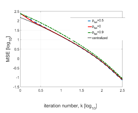
Figure 1: Estimated MSE versus iteration number $k$ for algorithm (2-B) with link failure probability $p_{\mathrm{fail}}=0$ (red, solid line); $0.5$ (blue, dashed line); and $0.9$ (green, dash-dot line). The Figure also shows the performance of the centralized stochastic gradient method in (34) (black, dotted line).

5 Conclusion

We considered a distributed stochastic gradient method for smooth strongly convex optimization. Through the analysis of the considered method, we established for the first time the order optimal $O(1/k)$ MSE convergence rate for the assumed optimization setting when the underlying network is randomly varying. Simulation example on $\ell_{2}$-regularized logistic losses corroborates the established $O(1/k)$ rate and suggests that the effect of the underlying network’s statistics on the $O(1/k)$ rate’s hidden constant is small.

References

• [1] S. Kar and J. M. F. Moura, “Convergence rate analysis of distributed gossip (linear parameter) estimation: Fundamental limits and tradeoffs,” IEEE Journal of Selected Topics in Signal Processing, Signal Processing in Gossiping Algorithms Design and Applications, vol. 5, no. 4, pp. 674 –690, Aug. 2011.
• [2] F. Bullo, J. Cortes, and S. Martinez, Distributed control of robotic networks: A mathematical approach to motion coordination algorithms.   Princeton University Press, 209.
• [3] A. Daneshmand, F. Facchinei, V. Kungurtsev, and G. Scutari, “Hybrid random/deterministic parallel algorithms for convex and nonconvex big data optimization,” IEEE Transactions on Signal Processing, vol. 63, no. 15, pp. 3914–3929, 2015.
• [4] I. Lobel and A. E. Ozdaglar, “Distributed subgradient methods for convex optimization over random networks,” IEEE Trans. Automat. Contr., vol. 56, no. 6, pp. 1291–1306, Jan. 2011.
• [5] I. Lobel, A. Ozdaglar, and D. Feijer, “Distributed multi-agent optimization with state-dependent communication,” Mathematical Programming, vol. 129, no. 2, pp. 255–284, 2011.
• [6] D. Jakovetic, J. Xavier, and J. M. F. Moura, “Convergence rates of distributed Nesterov-like gradient methods on random networks,” IEEE Transactions on Signal Processing, vol. 62, no. 4, pp. 868–882, February 2014.
• [7] K. Tsianos and M. Rabbat, “Distributed strongly convex optimization,” 50th Annual Allerton Conference onCommunication, Control, and Computing, Oct. 2012.
• [8] Z. J. Towfic, J. Chen, and A. H. Sayed, “Excess-risk of distributed stochastic learners,” IEEE Transactions on Information Theory, vol. 62, no. 10, Oct. 2016.
• [9] D. Yuan, Y. Hong, D. W. C. Ho, and G. Jiang, “Optimal distributed stochastic mirror descent for strongly convex optimization,” Automatica, vol. 90, pp. 196–203, April 2018.
• [10] N. D. Vanli, M. O. Sayin, and S. S. Kozat, “Stochastic subgradient algorithms for strongly convex optimization over distributed networks,” IEEE Transactions on network science and engineering, vol. 4, no. 4, pp. 248–260, Oct.-Dec. 2017.
• [11] A. Nedic and A. Olshevsky, “Stochastic gradient-push for strongly convex functions on time-varying directed graphs,” IEEE Transactions on Automatic Control, vol. 61, no. 12, pp. 3936–3947, Dec. 2016.
• [12] A. K. Sahu, D. Jakovetic, D. Bajovic, and S. Kar, “Distributed zeroth order optimization over random networks: A Kiefer-Wolfowitz stochastic approximation approach,” 2018, available at https://www.dropbox.com/s/kfc2hgbfcx5yhr8/MainCDC2018KWSA.pdf.
• [13] S. Kar, J. M. F. Moura, and H. V. Poor, “Distributed linear parameter estimation: Asymptotically efficient adaptive strategies,” SIAM J. Control and Optimization, vol. 51, no. 3, pp. 2200–2229, 2013.