Breathing mode frequency of a strongly interacting Fermi gas across the 2D-3D dimensional crossover

Abstract

We address the interplay between dimension and quantum anomaly on the breathing mode frequency of a strongly interacting Fermi gas harmonically trapped at zero temperature. Using a beyond mean-field, Gaussian pair fluctuation theory, we employ periodic boundary conditions to simulate the dimensionality of the system and impose a local density approximation, with two different schemes, to model different trapping potentials in the tightly-confined axial direction. By using a sum-rule approach, we compute the breathing mode frequency associated with a small variation of the trapping frequency along the weakly-confined transverse direction, and describe its behavior as functions of the dimensionality, from two- to three-dimensions, and of the interaction strength. We compare our predictions with previous calculations on the two-dimensional breathing mode anomaly and discuss their possible observation in ultracold Fermi gases of ⁶Li and ⁴⁰K atoms.

I Introduction

Low-lying collective excitations play a fundamental role in understanding many-body phenomena and the recent realization of ultracold atomic gases provides a unique setting for investigating various novel collective dynamics Bloch et al. (2008). In particular, low dimensional atomic Fermi gases (in one and two dimensions) at the crossover from a Bose-Einstein condensate (BEC) to a Bardeen-Cooper-Schrieffer (BCS) superfluid present a broad range of intriguing collective phenomena that are now being successfully studied from both theoretical and experimental perspectives Vogt et al. (2012); Hofmann (2012); Gao and Yu (2012); Taylor and Randeria (2012); Levinsen and Parish (2015); Mulkerin et al. (2017). Low-dimensional regimes are experimentally achieved by using a combination of harmonic oscillator (HO) traps Bloch et al. (2008); Chin et al. (2010), whose oscillating frequencies are tuned in order to reach both two-dimensional (2D) pancake Fenech et al. (2016); Hueck et al. (2018) and one-dimensional (1D) cigar traps Guan et al. (2013). Alternatively, a standing wave laser beam in a given selected direction can force the system into a quasi-2D pancake-like regime, where multiple almost independent 2D clouds are realized Ong et al. (2015); Cheng et al. (2016); Boettcher et al. (2016); Turlapov and Kagan (2017).

It is well known that the long-range order parameter is expected to be highly suppressed by fluctuations in low dimensions, however it is still possible to achieve superfluidity with a quasi-long-range order according to the Berezinskii-Kosterlitz-Thouless phase transition universality Berezinskiǐ (1971); Kosterlitz and Thouless (1972). The interest around low-dimensional quantum gases, in particular for the 2D case, is further emphasized by features that are known to have no classical counterpart. At low temperatures an interacting Fermi gas experiences mainly $s$-wave scattering, which are theoretically modeled by a contact interaction. It is straightforward to observe that in two dimensions the Hamiltonian of such a system is invariant under length scaling, however due to the contact interaction unphysical contributions at large momenta are included. The solution to this problem is to introduce an extra length scale upon renormalization, the scattering length $a_{{\rm 2D}}$, which breaks the scale invariance of the classical Hamiltonian and leads to the phenomenon of the so-called quantum anomaly Holstein (1993).

A well-known consequence due to the breaking of scale invariance in two-dimensional gases can be found when exciting the harmonically trapped cloud via collective excitations. Namely, a small perturbation of the transverse harmonic frequency $\omega_{\perp}$ induces a breathing mode excitation whose frequency is given by $\omega_{B}=2\omega_{\perp}$ Pitaevskii and Rosch (1997); Werner and Castin (2006). This classical result is modified when the quantum anomaly is considered. The breathing mode frequency gains a weak dependence on the scattering length and deviates from the classical value, $\omega_{B}=2\omega_{\perp}$, within a range of $5-10\%$ Olshanii et al. (2010); Hofmann (2012); Gao and Yu (2012). This should be contrasted with the case of a three-dimensional gas, in which the classical Hamiltonian is in general not invariant under length scaling. Due to the contact interaction we must also renormalize the Hamiltonian with the 3D scattering length, $a_{\text{3D}}$, and the breathing mode thus strongly depends on the scattering length. The only exception is the unitarity limit, where the scattering length diverges, $a_{\text{3D}}=\pm\infty$, and the quantum Hamiltonian becomes scale invariant. As a result of the restored scale invariance, the breathing mode does not depend on temperature Hou et al. (2013). In the 3D regime, for a unitary Fermi cloud in the highly pancake-like trapping potential, the scale invariant breathing mode takes $\omega_{B}=\sqrt{3}\omega_{\perp}$ Hu et al. (2014); De Rosi and Stringari (2015). It is of great interest to study how the breathing mode frequency evolves at the dimensional crossover from 3D to 2D, while aiming for the realization of a truly 2D gas.

In this work, motivated by the recent experimental activities at Swinburne University of Technology Pep , we address the role of dimension and interaction on the breathing mode frequency and the quantum anomaly. The suppressed superfluid order parameter in low dimensions requires a beyond mean-field (MF) treatment Tempere and P.A. (2012); Mulkerin et al. (2017), which is possible when we consider periodic boundary conditions (PBC) in the axial direction Toniolo et al. (2017). Moreover, the effect of harmonic trapping in the transverse direction on the integrated 2D density distribution can be well described by a local density approximation (LDA). We describe the breathing mode frequency for a given pair of parameters: a length that tunes the dimension and a scattering length that sets the interaction strength. By using a sum-rule approach, in the spirit of Ref. Menotti and Stringari (2002), we determine the breathing mode frequency while changing the dimensional regime and tuning the scattering length. We further address a comparison with the previous results of the breathing mode frequency in the purely 2D regime Hofmann (2012); Gao and Yu (2012); Taylor and Randeria (2012). Our predictions could be readily examined in future cold-atom experiments with fermionic ⁶Li and ⁴⁰K atoms.

The paper is set out as follows: in Sec. II.1 we go through the beyond-MF, Gaussian pair fluctuation (GPF) theory to study a homogeneous strongly interacting Fermi gas with periodic boundary conditions, and in Sec. II.2 we introduce two different LDA schemes to account for different axial confinements. In Sec. II.4 we briefly derive the sum-rule for the breathing mode frequency calculations, which are extensively addressed in Appendix A, for the sake of clarity. Finally in Sec. III we show the behavior of the breathing mode frequency in various dimensional regimes and the comparison with previous 2D results.

II Theoretical models

II.1 Homogeneous strongly interacting Fermi gases at the dimensional crossover

Following our previous work in Ref. Toniolo et al. (2017), we model a two-component spin balanced Fermi gas near a broad Feshbach resonance via a two-body contact interaction. In order to describe the dimensional crossover, we split the spatial coordinates into in-plane $\mathbf{x}=(x,y)$ and axial $z$ components, combined in the short-hand notation $(\mathbf{x},z)$. The grand canonical single channel Hamiltonian reads Randeria et al. (1989),

$$\begin{split}\mathcal{H}=\sum_{\sigma=\uparrow,\downarrow}&\psi_{\sigma}^{\dagger}(\mathbf{x},z)\left(-\frac{\hbar^{2}}{2m}\nabla^{2}-\mu\right)\psi_{\sigma}(\mathbf{x},z)\\ &-U_{0}\psi_{\uparrow}^{\dagger}(\mathbf{x},z)\psi_{\downarrow}^{\dagger}(\mathbf{x},z)\psi_{\downarrow}(\mathbf{x},z)\psi_{\uparrow}(\mathbf{x},z),\end{split}$$ (1)

where $\psi_{\sigma}$ are the annihilation field operators for the (pseudo-)spin populations labeled by $\sigma=\uparrow,\downarrow$, $\mu$ is the chemical potential, $m$ is the mass of the fermions, and $U_{0}>0$ is the bare interaction strength of the contact potential. We introduce the Hubbard-Stratonovich auxiliary bosonic field, $\hat{\Delta}(x)=U_{0}\psi_{\downarrow}(\mathbf{x},z)\psi_{\uparrow}(\mathbf{x},z)$, and we perform a saddle point approximation with the mean-field order parameter and the fluctuation bosonic field Hu et al. (2006); Diener et al. (2008), $\hat{\Delta}(x)=\Delta+\hat{\phi}(\mathbf{x},z)$. This approximation allows us to directly compute the thermodynamic potential up to second order in the fluctuation, $\Omega=\Omega_{{\rm MF}}+\Omega_{{\rm GPF}}$, where at the MF level we have,

$$\frac{\Omega_{\text{MF}}}{V}=\frac{\Delta^{2}}{U_{0}}+\frac{1}{V}\sum_{\mathbf{k},k_{z}}(\xi_{\mathbf{k},k_{z}}-E_{\mathbf{k},k_{z}}),$$ (2)

where $V$ is the volume of the system and we have introduced the BCS theory notation, slightly modified for the dimensional crossover, for a generic momentum $(\mathbf{k},k_{z})$: we define $\xi_{\mathbf{k},k_{z}}=\varepsilon_{\mathbf{k}}+\varepsilon_{k_{z}}-\mu$ and $E_{\mathbf{k},k_{z}}=\sqrt{\xi_{\mathbf{k},k_{z}}^{2}+\Delta^{2}}$. The GPF contribution to the thermodynamic potential, at finite temperature $k_{B}T=\beta^{-1}$, is

$$\Omega_{\text{GPF}}=-\frac{1}{\beta}\ln\int\mathcal{D}\phi^{*}\mathcal{D}\phi\exp\left[\mathcal{S}_{\text{GPF}}(\phi^{*},\phi)\right],$$ (3)

where $k_{B}$ is the Boltzmann constant and the GPF action, $\mathcal{S}_{\text{GPF}}$, can be written as

$$\mathcal{S}_{\text{GPF}}=\frac{\beta V}{2}\sum_{Q}\begin{pmatrix}\phi_{Q}^{*}&\phi_{-Q}\end{pmatrix}\mathbf{M}(Q)\begin{pmatrix}\phi_{Q}\\ \phi_{-Q}^{*}\end{pmatrix}.$$ (4)

We have introduced the multi-index notation $Q\equiv(\mathbf{q},q_{z},\operatorname{i}q_{\nu})$ with momenta, $(\mathbf{q},q_{z})$, of the fluctuation field, $\phi$, and the bosonic Matsubara frequencies $q_{\nu}=2\pi\nu/\beta$, for all $\nu\in\mathbb{Z}$. The matrix operator $\mathbf{M}$ at zero temperature can be written,

$$\mathbf{M}_{11} = \frac{1}{U_{0}}+\frac{1}{V}\sum_{\mathbf{k},k_{z}}\left(\frac{u_{+}^{2}u_{-}^{2}}{\operatorname{i}q_{\nu}-E_{+}-E_{-}}-\frac{v_{+}^{2}v_{-}^{2}}{\operatorname{i}q_{\nu}+E_{+}+E_{-}}\right),$$

$$\mathbf{M}_{12} = \frac{1}{V}\sum_{\mathbf{k},k_{z}}\left(-\frac{u_{+}u_{-}v_{+}v_{-}}{\operatorname{i}q_{\nu}-E_{+}-E_{-}}+\frac{u_{+}u_{-}v_{+}v_{-}}{\operatorname{i}q_{\nu}+E_{+}+E_{-}}\right),$$ (5)

$\mathbf{M}_{21}\left(Q\right)=\mathbf{M}_{12}\left(Q\right)$ and $\mathbf{M}_{22}\left(Q\right)=\mathbf{M}_{11}\left(-Q\right)$. Here, we use the notations Hu et al. (2006); Diener et al. (2008); He et al. (2015)

$$u_{\pm}^{2}=1-v_{\pm}^{2}=\frac{1}{2}\left(1+\frac{\xi_{\pm}}{E_{\pm}}\right),$$ (6)

with $E_{\pm}=\sqrt{\xi_{\pm}^{2}+\Delta^{2}}$ and $\xi_{\pm}\equiv\xi_{\mathbf{k}\pm\frac{\mathbf{q}}{2},k_{z}\pm\frac{q_{z}}{2}}$. At zero temperature, for $\beta\rightarrow\infty$, we can Wick rotate the Matsubara frequencies Diener et al. (2008); He et al. (2015), $\operatorname{i}q_{\nu}\mapsto\omega$, swapping the sum on $\operatorname{i}q_{\nu}$ with an integration on $\omega$,

$$\Omega_{\text{GPF}}=\frac{1}{V}\sum_{\mathbf{q},q_{z}}\int_{0}^{\infty}\frac{d\omega}{2\pi}\ln\Gamma^{-1}(\mathbf{q},q_{z},\omega),$$ (7)

where

$$\Gamma^{-1}(Q)=\frac{\mathbf{M}_{11}(Q)\mathbf{M}_{11}(-Q)-\mathbf{M}_{12}(Q)^{2}}{\mathbf{M}_{11}^{C}(Q)\mathbf{M}_{11}^{C}(-Q)},$$ (8)

and we have introduced an additional term to converge the integrations Diener et al. (2008); He et al. (2015),

$$\mathbf{M}_{11}^{C}\left(Q\right)=\frac{1}{U_{0}}+\frac{1}{V}\sum_{\mathbf{k},k_{z}}\frac{u_{+}^{2}u_{-}^{2}}{\operatorname{i}q_{\nu}-E_{+}-E_{-}}.$$ (9)

The dispersion relation of the bosonic field should be gapless, hence we determine the order parameter, $\Delta$, at the MF level by solving the gap equation

$$\mathbf{M}_{11}(Q=0)-\mathbf{M}_{12}(Q=0)=0,$$ (10)

or more explicitly,

$$\frac{1}{U_{0}}-\frac{1}{V}\sum_{\mathbf{k},k_{z}}\frac{1}{2E_{\mathbf{k},k_{z}}}=0.$$ (11)

In the spirit of Ref. Toniolo et al. (2017), we introduce the tuning parameters of the dimensional crossover as follows: the in-plane coordinates are sent to the thermodynamic limit, while we require PBC to hold on the axial direction. The characteristic PBC length $l_{z}$ tunes the dimensional crossover from the 3D (large $l_{z}$) limit towards the 2D (small $l_{z}$) regime. We define the characteristic Fermi momentum $k_{F}$ and Fermi energy $\varepsilon_{F}=\hbar^{2}k_{F}^{2}/(2m)$ from the free Fermi density $n_{f}$. That is, for a fixed box length $l_{z}$, we take the discretization of momenta in the $z$ direction, $k_{z}=2\pi N_{z}/l_{z}$, for any integer $N_{z}$. The free Fermi density is then given by Toniolo et al. (2017),

$$n_{f}=\frac{1}{2\pi l_{z}}\sum_{N_{z}=-N_{\text{max}}}^{N_{\text{max}}}\left[k_{F}^{2}-\left(\frac{2\pi N_{z}}{l_{z}}\right)^{2}\right],$$ (12)

where $N_{\text{max}}$ is the largest natural number smaller than $k_{F}l_{z}/(2\pi)$. In the 2D and 3D limits, the Fermi momentum $k_{F}$ should approach respectively their limiting values, $k_{F}^{\text{2D}}$ and $k_{F}^{\text{3D}}$, which can be defined by the 2D and 3D free Fermi densities $n_{\text{2D}}=n_{f}l_{z}$ and $n_{\text{3D}}=n_{f}$ in the usual way. For convenience, we introduce the dimensional crossover tuning parameter via the 3D Fermi momentum $k_{F}^{\text{3D}}$ Toniolo et al. (2017):

$$\eta\equiv k_{F}^{\text{3D}}l_{z}.$$ (13)

We renormalize the bare interaction strength, $U_{0}$, by requiring that the two-body $T$-matrices in the quasi-2D and 3D regimes match when $l_{z}\rightarrow\infty$, which defines a quasi-2D binding energy $B_{0}$ Yamashita et al. (2014); Petrov and Shlyapnikov (2001) as a function of $a_{\text{3D}}$, with an explicit dependence on $l_{z}$,

$$B_{0}=\frac{4\hbar^{2}}{ml_{z}^{2}}\operatorname{arcsinh}^{2}\left[\frac{e^{l_{z}/(2a_{\text{3D}})}}{2}\right].$$ (14)

The binding energy fixes the BCS-BEC crossover tuning parameter $l_{z}/a_{\text{3D}}$ which spans from negative (BCS) to positive (BEC) values. When $l_{z}\rightarrow 0$, the quantity $B_{0}/(2\varepsilon_{F})$ is well defined and spans the 2D BCS-BEC crossover by introducing

$$-\text{ln}\left(k_{F}^{\text{2D}}a_{\text{2D}}\right)=-\text{ln}\sqrt{\frac{B_{0}}{2\varepsilon_{F}}}.$$ (15)

Finally, we can define the density of the system as a function of two parameters, namely the chemical potential, $\mu$, and the PBC length, $l_{z}$, via the number equation

$$n(\mu,l_{z})=-\frac{1}{V}\frac{\partial\Omega(\mu,l_{z})}{\partial\mu}\Big{|}_{\mu;\Delta(\mu)},$$ (16)

where, for each pair $(\mu,l_{z})$, $\Delta(\mu)$ means we have solved the gap equation before taking the derivative.

II.2 Local density approximation

As we shall see, the breathing mode frequency in the transverse plane can be calculated from the integrated 2D density or the so-called column density,

$$n_{2D}(\mathbf{\rho=}\sqrt{x^{2}+y^{2}})=\int dz\ n(\rho,z),$$ (17)

by using a sum-rule approach. We now discuss how to determine the column density using the uniform density equation of state Eq. (16) and the LDA approach, in the presence of a harmonic trapping potential in the $xy$-plane and two types of confinement in the axial direction:

$$V_{T}\left(\rho,z\right)=\frac{1}{2}m\omega_{\perp}^{2}\rho^{2}+\left\{\begin{array}[]{c}V_{\infty}\Theta\left[\left|z\right|-l_{z}/2\right],\\ \frac{1}{2}m\omega_{z}^{2}z^{2},\end{array}\right.$$ (18)

where the potential $V_{\infty}\Theta[\left|z\right|-l_{z}/2]$, with $V_{\infty}\rightarrow\infty$ and step function $\Theta(x)$, simulates a hard-wall box confinement that may be realized in future experiments and $m\omega_{z}^{2}z^{2}/2$ is the standard harmonic trapping potential Fenech et al. (2016); Hueck et al. (2018). In both cases, the trap aspect ratio, characterized by $\lambda=\hbar/(m\omega_{\bot}l_{z}^{2})$ under the hard-wall confinement and $\lambda=\omega_{z}/\omega_{\bot}$ in the case of harmonic potential, should be much larger than $1$.

To calculate the column density, let us first clarify the different dimensional regimes. In Ref. Toniolo et al. (2017) the dimensional crossover of a PBC system, which could be used to describe a nearly homogeneous quasi-2D Fermi cloud under hard-wall confinement, is split into three regimes. These are distinguished through the position of the maximum of the superfluid critical velocity, $v_{c}^{\max{}}$, which has a non-trivial dependence on the dimensional parameter $\eta$. For $\eta\leq 2$ the maximum of the superfluid velocity is logarithmically dependent on $\eta$, and we denote this as the 2D regime. The maximum of the superfluid velocity becomes linear in $\eta$ when $\eta\geq 8$ marking the 3D regime. The non-monotonic region contained between the 2D and 3D regimes is the quasi-2D regime. For further details on other choices of characterizing the crossover, see Supplemental Material in Ref. Toniolo et al. (2017).

To understand the dimensional crossover in the presence of a tight harmonic axial trapping potential, we may determine an equivalent PBC length scale by approximating

$$l_{z}\sim l_{z}^{\text{HO}}=\sqrt{\frac{\hbar}{m\omega_{z}}}.$$ (19)

By doing so, Eq. (16) depends on $l_{z}$ as an external parameter fixed by the axial harmonic frequency $\omega_{z}$. We then compare $l_{z}$ with $k_{F}^{\text{3D}}$ and obtain a simple relation to compare the PBC to the harmonically trapped system,

$$\eta\sim k_{F}^{\text{3D}}l_{z}^{\text{HO}}=\sqrt{\frac{2\varepsilon_{F}^{\text{3D}}}{\hbar\omega_{z}}}.$$ (20)

The single-particle criterion for the harmonically trapped Fermi gas in the 2D regime is given by requiring: (1) $k_{B}T\ll\varepsilon_{F}$ to avoid thermal excitations of the axial harmonic oscillator ground state, and (2) $\hbar\omega_{z}>\varepsilon_{F}$ to ensure that the whole system is contained in the ground state. By solving $n_{\text{3D}}=n_{f}$, we see that from Eq. (12) we always have $\varepsilon_{F}<\varepsilon_{F}^{\text{3D}}$ for $\eta<3\pi/2$. By taking $k_{F}^{\text{3D}}l_{z}^{\text{HO}}<\sqrt{2}$, we may interpret $k_{F}^{\text{3D}}l_{z}<\sqrt{2}$ as a good approximate regime of the 2D limit for the trapped case. We denote this regime as the harmonic oscillator (HO) 2D regime. This distinguishes between the PBC 2D regime and the 2D regime for a harmonically trapped Fermi gas.

In Fig. 1 and Fig. 2, we show the the dimensional regimes as a function of $\eta$ and differentiate the PBC and harmonically trapped 2D regimes using different colors. We note that, the harmonically trapped Fermi gas density has been experimentally studied Dyke et al. (2011, 2016). A plateau in the column density has been observed, by decreasing the total number of atoms to reach the 2D regime at a given 3D $s$-wave scattering length Dyke et al. (2016). By converting the experimentally determined threshold number density to the dimensional parameter (i.e., using Eq. (20)), we qualitatively determine the boundary of the HO 2D regime as a function of the interaction strength $(k_{F}^{3D}a_{3D})^{-1}$. This is illustrated in Fig. 3(a) by the pink shaded region.

II.2.1 The in-plane LDA

For a hard-wall confinement along the axial direction, the density distribution is nearly uniform as a function of $z$ (i.e., see Supplemental Material in Ref. Toniolo et al. (2017)). Our theory of a homogeneous strongly interacting Fermi gas at the dimensional crossover, as outlined in Sec. II.1, could be quantitatively applicable. Thus, we must have the column density,

$$n_{2D}\left[\mu\left(\rho\right)\right]=l_{z}n\left[\mu\left(\rho\right),l_{z}\right],$$ (21)

where $n[\mu(\rho),l_{z}]$ can be calculated using Eq. (16), once a local chemical potential $\mu(\rho)$ at the radius $\rho$ is provided. For a slowly varying transverse potential $m\omega_{\perp}^{2}\rho^{2}/2$, the assignment of a local chemical potential is a well-established approximation, as the surface energy related to the potential change becomes negligible compared to the bulk energy scale. This treatment is known as the Thomas-Fermi approximation or LDA. More explicitly, we have a local chemical potential in Eq. (21):

$$\mu\left(\rho\right)=\mu_{g}-\frac{1}{2}m\omega_{\perp}^{2}\rho^{2},$$ (22)

where the chemical potential at the trap center $\mu_{g}$ should be adjusted to yield the total number of atoms $N$, i.e.,

$$N=2\pi\int_{0}^{\infty}\rho n_{2D}\left(\rho\right)d\rho.$$ (23)

In the following, this LDA scheme is referred to as the in-plane LDA.

II.2.2 The all-direction LDA

The situation becomes much more complicated for a harmonic axial trapping potential. This soft-wall potential allows density variation in the $z$-direction. It is clear that the density distribution of the Fermi cloud could have very different $z$-dependence at different dimensional regimes. Deep in the 2D regime, we anticipate that the density profile may be approximated by,

$$n\left[\mu\left(\rho,z\right)\right]\simeq n_{2D}\left(\rho\right)\left|\Phi_{0}\left(z\right)\right|^{2},$$ (24)

where $\Phi_{0}\left(z\right)$ is the ground state HO wave-function along the $z$-direction that is normalized to unity, i.e., $\int dz\left|\Phi(z)\right|^{2}=1$. As the confinement is tight along the $z$-direction, we are of course not allowed to define a $z$-dependent local chemical potential and use Eq. (16) to calculate $n_{2D}\left(\rho\right)$. However, there is an interesting observation in the deep 2D regime. As all the atoms are confined in the ground state of the tight confinement, the in-plane motion of the atoms should be universally described by the same 2D Hamiltonian, regardless of the detailed form of the confinement. This implies that the 2D density equation of state $n_{2D}(\mu)$ should be independent of the form of tight confinement, as far as the confinement gives the same 2D binding energy or 2D scattering length. Therefore, we could still use Eq. (21) to determine the column density, provided that the length $l_{z}$ is accurately approximated in the presence of the axial harmonic trapping potential.

Away from the deep 2D limit, we expect this approximation to increasingly fail in describing the harmonically confined system when the dimensional parameter $\eta$ moves towards the quasi-2D and 3D regimes of the PBC confined model. Fortunately, in the deep 3D regime, the axial trapping potential $m\omega_{z}^{2}z^{2}/2$ becomes slowly varying in space as well. In this case, we may implement an all-direction LDA scheme, by setting

$$\mu(\rho,z)=\mu_{g}-\frac{1}{2}m\omega_{\perp}^{2}\rho^{2}-\frac{1}{2}m\omega_{z}^{2}z^{2}.$$ (25)

We can introduce a new set of variables, $\xi^{2}=\rho^{2}+\lambda^{2}z^{2}$ and $\tan\psi=\lambda z/\rho$, and rewrite the chemical potential as a function of $\xi$ only, $\mu(\xi)=\mu_{g}-m\omega_{\perp}^{2}\xi^{2}/2$, for a fixed aspect ratio $\lambda$. The number of particles, $N$, of the system approximated with LDA, in cylindrical coordinates, is given by

$$N=2\pi\int_{-\infty}^{\infty}dz\int_{0}^{\infty}d\rho\ \rho\ n\left[\mu(\rho,z)\right].$$ (26)

The above equation can be used as well for the in-plane LDA to replace Eq. (23), if we require $n(\rho,l_{z})=n(\rho)$ when $z\in[-l_{z}/2,l_{z}/2]$ and $n(\rho,l_{z})=0$ otherwise.

As a brief summary, in the presence of an axial harmonic trapping potential, we will use the in-plane LDA in the 2D regime and the all-direction LDA in the 3D regime, as an accurate description for the column density equation of state. At the 2D-3D crossover, we take interpolation between these two limits and obtain a qualitative description.

II.3 Polytropic column density equation of state

In some limiting cases, the column density may be well approximated by a polytropic form

$$\mu(n_{2D})\propto n_{2D}^{\gamma},$$ (27)

which, as we shall see, provides a significant simplification in understanding the breathing mode. For example, in the deep 2D limit, the weak violation of the scale invariance implies that Taylor and Randeria (2012); Hofmann (2012)

$$\gamma_{2D}\sim 1,$$ (28)

regardless of the type of the tight axial confinement. In the 3D regime, if we consider a unitary Fermi gas, the well-known relation $\mu=\xi\varepsilon_{F}\propto n^{2/3}$, where $\xi$ is the Bertsch parameter Bloch et al. (2008), gives rise to,

$$\gamma_{3D}^{(\textrm{HW})} = 2/3,$$ (29)

$$\gamma_{3D}^{(\textrm{HO})} = 1/2,$$ (30)

where the superscripts “HW” and “HO” distinguish the hard-wall and harmonic axial trapping potentials. We note that, the polytropic coefficient with harmonic axial trapping potential decreases to $1/2$, due to the implementation of the LDA along the $z$-axis Hu et al. (2014); De Rosi and Stringari (2015).

II.4 Breathing mode frequency

Once we calculate the density as a function of the chemical potential and position, the collective oscillations of the Fermi gas can be derived from the hydrodynamic treatment of the system Griffin et al. (1997); Menotti and Stringari (2002). These techniques have been successfully employed to predict a large variety of collective oscillations for fermionic systems Csordás and Adam (2006); Taylor et al. (2008); De Rosi and Stringari (2015). In this work, we adopt the commonly-used sum-rule method Stringari (1998); Gao and Yu (2012), where the breathing mode frequency, $\omega_{B}$, is given by the ratio

$$\hbar^{2}\omega_{B}^{2}=\frac{M_{1}}{M_{-1}}.$$ (31)

$M_{1}$ is given by the energy weighted moment of the density (second order central momentum of the density distribution), $M_{1}=2N\hbar^{2}\langle\rho^{2}\rangle/m$, and $M_{-1}$ is related to a perturbation of the radial coordinate, $M_{-1}=N\delta\langle\rho^{2}\rangle/\varepsilon$, where $\delta\langle\rho^{2}\rangle$ represents the second order momentum when the transverse harmonic oscillator potential is perturbed by $-\varepsilon\rho^{2}$. The expectation value of the radius squared is given by,

$$\langle\rho^{2}\rangle\propto\int_{0}^{\infty}\rho^{3}n_{2D}(\rho)d\rho$$ (32)

and we can recast the perturbation of the radial coordinate to a perturbation of $\omega_{\perp}$, obtaining the closed form Menotti and Stringari (2002)

$$\hbar^{2}\omega_{B}^{2}=-2\langle\rho^{2}\rangle\left[\frac{d\langle\rho^{2}\rangle}{d(\omega_{\perp}^{2})}\right]^{-1}.$$ (33)

From Eq. (33) we observe that we need to know $\langle\rho^{2}\rangle$ up to any constant which doesn’t implicitly depend on $\omega_{\perp}$. We show in Appendix A that the number of particles falls out of the computation of $\omega_{B}$ when we dimensionalize the results with the transverse frequency $\omega_{\perp}$. The right-hand-side of Eq. (33) is expected to be linear in $\omega_{\perp}^{2}$ and return a constant when we evaluate $\omega_{B}/\omega_{\perp}$ (for further details see Appendix A).

It is worth noting that, when the equation of state has a polytropic form, $\mu(n_{2D})\propto n_{2D}^{\gamma}$, the sum-rule approach for evaluating the breathing mode frequency become exact Hu et al. (2014); De Rosi and Stringari (2015). It gives (see Appendix A for the derivation),

$$\frac{\omega_{B}}{\omega_{\perp}}=\sqrt{2+2\gamma}.$$ (34)

Therefore, we anticipate that in different dimensional regimes the breathing mode frequency may behave like,

$$\omega_{B,2D} \sim 2\omega_{\perp},$$ (35)

$$\omega_{B,3D}^{(\textrm{HW})} = \sqrt{10/3}\omega_{\perp},$$ (36)

$$\omega_{B,3D}^{(\textrm{HO})} = \sqrt{3}\omega_{\perp}.$$ (37)

The latter two results hold for a unitary Fermi gas only.

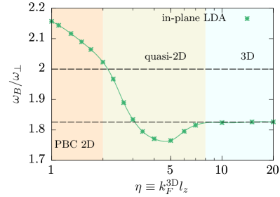
Figure 1: The breathing mode frequency $\omega_{B}$ in units of $\omega_{\perp}$ as a function of the dimensional crossover tuning parameter $\eta\equiv k_{F}^{\text{3D}}l_{z}$, when the BCS-BEC crossover is tuned at unitarity with $a_{\text{3D}}=\infty$. Here, we consider the hard-wall confinement along the axial direction. The upper and bottom dashed lines are the scale invariant predictions in the 2D and 3D limits, $\omega_{B,2D}=2\omega_{\perp}$ and $\omega_{B,3D}^{(\textrm{HW})}=\sqrt{10/3}\omega_{\perp}\simeq 1.83\omega_{\perp}$, respectively.

III Results

We now report the breathing mode frequency at the dimensional crossover and consider the two different types of axial confinement: the hard-wall box trapping potential and soft-wall harmonic potential. The former case is only briefly discussed, as the hard-wall confinement is yet to be experimentally demonstrated. Hereafter, without any confusions we use $k_{F}^{3D}\equiv(3\pi^{2}n_{0})^{1/3}$ to represent the 3D Fermi momentum of an interacting Fermi gas at the trap center with density $n_{0}\equiv n(\rho=0,z=0)$. In our case of considering two different axial confinements, this turns out to be a more convenient option than the use of the 3D Fermi momentum of an ideal Fermi gas at the trap center.

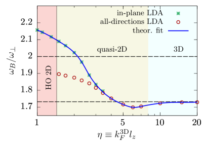
Figure 2: The breathing mode frequency $\omega_{B}$ divided by $\omega_{\perp}$ as a function of the dimensional crossover tuning parameter $\eta\equiv k_{F}^{\text{3D}}l_{z}$ when the BCS-BEC crossover is tuned at unitarity with $a_{\text{3D}}=\infty$. The results from the in-plane LDA (green stars) and all-direction LDA (brown circles) schemes are merged when the lines match to form a qualitative fit (blue solid). The dimensional crossover is divided into the three dimensional regimes as in Ref. Toniolo et al. (2017) and the HO 2D regime is determined using the experimental criterion of Ref. Dyke et al. (2011) for a 2D harmonically trapped Fermi gas. The upper and bottom dashed lines are the scale invariant predictions in the 2D and 3D limits, $\omega_{B,2D}=2\omega_{\perp}$ and $\omega_{B,3D}^{(\textrm{HO})}=\sqrt{3}\omega_{\perp}\simeq 1.73\omega_{\perp}$, respectively.

III.1 The hard-wall axial confinement

In Fig. 1 we present the breathing mode frequency of a unitary Fermi gas at the dimensional crossover, in the presence of a hard-wall axial confinement. The mode frequency is calculated by using the in-plane LDA, as a function of the dimensional parameter $\eta$ expanding from the PBC 2D regime when $\eta\leq 2$ to the 3D regime when $\eta\geq 8$. As our GPF theory provides reliable equation of state at the dimensional crossover, we anticipate that our prediction on the breathing mode frequency is reliable. In the PBC 2D regime, the mode frequency is larger than $2\omega_{\perp}$, indicating a pronounced quantum anomaly. As we move to the quasi-2D regime, the frequency decreases rapidly, reaches a minimum at $\eta\sim 5$ and finally approaches the 3D limiting value of $\omega_{B,3D}^{(\textrm{HW})}=\sqrt{10/3}\omega_{\perp}$ at $\eta\geq 10$.

III.2 The harmonic axial confinement

In Fig. 2, we show the dimensional crossover of the breathing mode again for the unitary Fermi gas, but with the harmonic axial trapping potential. Here, the 3D regime is reached as before when $\eta\geq 8$, and the HO 2D regime is realized when $\eta\leq\sqrt{2}$. As we mentioned earlier, we calculate the breathing mode frequency using the in-plane LDA scheme near the 2D regime (green stars) and using the all-direction LDA scheme close to the 3D regime (brown circles). The in-plane LDA fails to describe the 3D regime, so we show its prediction at $\eta<4$ only. The all-direction LDA scheme fails in the 2D regime, since the ground state wave-function in the axial direction is essentially a Gaussian. As a guide to the eyes, we combine the two different LDA schemes with the blue solid line, and this qualitatively describes the breathing mode frequency in two mutually exclusive regions of the dimensional crossover. By increasing $\eta$, we find that the mode frequency shows the same behavior as in the case of the hard-wall confinement: it decreases quickly away from the 2D regime, exhibits a minimum in the quasi-2D regime and then saturates to a 3D limiting value, which is $\omega_{B,3D}^{(\textrm{HO})}=\sqrt{3}\omega_{\perp}\simeq 1.73\omega_{\perp}$ in the presence of the harmonic trapping potential.

We now turn to describe the behavior of the breathing mode frequency at the BEC-BCS crossover other than the unitarity limit. For this purpose, we need to distinguish different interacting regimes and clarify the so-called unitarity regime. In all the previous discussions, the unitarity regime and an infinite 3D scattering length are two exchangeable terminologies, both of which can be used without any confusions in the 3D regime. Away from the 3D limit, however it seems more intuitive to define the unitarity regime as the regime where the coherence length of Cooper pairs is comparable to the inter-particle distance and where the fermionic superfluidity is most robust.

It is worth noting that, fixing a constant 3D interacting parameter is the best way to compare with experimental results, however from a theoretical point of view we want an interaction parameter which probes the same interacting regime as a function of $\eta$. If we choose the simple condition for the 3D interacting parameter, i.e. $(k_{F}^{\text{3D}}a_{\text{3D}})^{-1}$ fixed equal to a constant, when we span the dimensional parameter $\eta$, the system crosses different interacting regimes. For example, in Fig. 1 where we have set the 3D scattering length to infinity, we are in the unitarity regime in the 3D limit while the system enters the BEC regime for the quasi-2D and 2D regimes. In the HO 2D case, the system is even in the deep BEC regime Dyke et al. (2011). From now on, we fix the unitary regime through the maximum of the critical velocity, as described in our previous work in determining the dimensional regimes Toniolo et al. (2017). This is a reasonable definition, since the maximum critical velocity implies the most robust fermionic superfluidity.

Figure 3(a) displays the choices made for the BCS (dashed-dotted green line) and BEC (dashed blue line) crossover regimes, in which the two lines are obtained by vertically shifting the maximum critical velocity curve down and up by some amounts. These choices appear to be optimal since they both span the 2D and 3D limits ($\eta=2$ and $\eta=20$ respectively). For the 2D limit both the PBC 2D regime and the HO 2D regime are reached, and converting the scattering length to its 2D counterpart, $\ln(k_{F}^{\text{2D}}a_{\text{2D}})$, we observe that it spans the relevant part of BCS-BEC crossover.

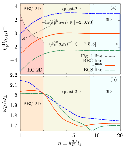
Figure 3: (a) The interaction parameter $(k_{F}^{\text{3D}}a_{\text{3D}})^{-1}$, as a function of $\eta$, fixed by the BCS, BEC, and $v_{c}^{\max{}}$ lines in order to span the dimensional crossover and maintain the system in the BCS (dashed dotted green), unitarity (solid red), and BEC (dashed blue) interacting regimes. According to Ref. Toniolo et al. (2017) the solid red line is taken to be a good criterion to distinguish the BCS and BEC regimes. (b) we show the breathing mode frequency $\omega_{B}$ in units of $\omega_{\perp}$ as a function of the dimensional crossover parameter $\eta\equiv k_{F}^{\text{3D}}l_{z}$ for the BCS (dashed dotted green), unitarity (solid red), and BEC (dashed blue) interacting regimes.

In Fig. 3(b) we plot the ratio $\omega_{B}/\omega_{\perp}$ in the different interacting regimes as per Fig. 3(a), the BCS (dashed dotted green), unitarity (solid red), and BEC (dashed blue) regimes. We see that the deviation of the breathing mode from the classic result, $\omega_{B}=2\omega_{\perp}$, appears when the 2D region is entered. Since the quantum anomaly is due to the presence of the renormalization energy $B_{0}$, which tends to vanish while approaching the BCS regime, we observe a strong deviation in the BEC regime (dashed blue) which is progressively reduced in the unitarity regime (solid red). Qualitatively, the fit between the in-plane and all-direction LDA results drop from $2\omega_{\perp}$ to a range of values around the 3D unitarity limit, $\omega_{B}=\sqrt{3}\omega_{\perp}$. The unitarity results (red-solid) converge to this value, while as remarked in Ref. Hu et al. (2004), the BEC regime provides a larger value of $\omega_{B}$, and in the BCS limit there is a non trivial behavior below $\omega_{B}=\sqrt{3}\omega_{\perp}$.

III.3 Quantum anomaly in the deep 2D regime

Focusing on the 2D regime, i.e. $\eta=1$, we compare our results with previous two-dimensional studies Hofmann (2012); Gao and Yu (2012). Since the choice $\eta=1$ and a large range of values of $\ln(k_{F}^{\text{2D}}a_{\text{2D}})$ are contained both in the PBC 2D and harmonic oscillator 2D regime, we compare the anomaly through the quantity $\delta\omega_{B}/\omega_{\perp}$, where $\delta\omega_{B}=\omega_{B}-2\omega_{\perp}$.

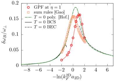
Figure 4: The quantum anomaly deviation $\delta\omega_{B}=\omega_{B}-2\omega_{\perp}$ of the breathing mode frequency $\omega_{B}$ in units of the transverse harmonic trapping frequency $\omega_{\perp}$. Our results (red circles) are obtained by applying the in-plane LDA for the PBC confined 2D Fermi gas ($\eta=1$) at the GPF level. For comparison, we show also the polytropic fit from Ref. Hofmann (2012) (dashed green), the sum rule results from Ref. Gao and Yu (2012) (orange squares), and the zero temperature analytic predictions for the far BCS (solid black) and BEC (dashed-dotted black) regimes.

We observe that the qualitative behavior of the quantum anomaly is recovered by our data, and the maximum of the deviation, $\delta\omega_{B}$, is approximately the same height of Ref. Gao and Yu (2012). The shift of the anomaly to the BEC side in our results is due to either the GPF contribution to the global chemical potential $\mu_{g}$ in comparison to the quantum Monte Carlo schemes, or that for $\eta=1$ the range of $\ln(k_{F}^{\text{2D}}a_{\text{2D}})$ is shifted with respect to the exact 2D case when we consider the exact 2D limit.

IV Conclusions

In conclusions, we have characterized the breathing mode of a strongly interacting Fermi gas at the dimensional crossover from two- to three-dimensions, as a function of the interatomic interaction strength. Using two schemes for the local density approximation, through the hydrodynamic formalism and sum rules we are able to calculate the breathing mode within a beyond mean-field, gaussian pair fluctuation theory. Two kinds of tight axial confinements have been considered: a hard-wall box potential and a soft-wall harmonic trapping potential. In both cases, we have shown that the quantum anomaly will be visible in the breathing mode frequency as we approach two dimensions in the strongly interacting regime. We have compared our breathing mode anomaly in two-dimensions directly to the previous predictions based quantum Monte Carlo simulations and have found a good agreement. As the dimension of the system changes to quasi-2D, the breathing mode decreases in a non-monotonic way, and towards the 3D regime, it saturates to the anticipated scaling invariant values, in the case of an infinite three-dimensional scattering length.

Our results may be quantitatively applicable to the case of the hard-wall axial confinement, where the density distribution along the axial direction is more or less uniform. For the case of an axial harmonic trapping potential, we instead anticipate that our results provide a good qualitative description, due to ambiguity in interpreting the length of axial confinement $l_{z}$. We are now working on the density equation of state by explicitly including harmonic trapping in the axial direction, and aim to provide a more quantitative description.

Appendix A Sum rule for the breathing mode frequency

According to Eq. (33), we need to know $\langle\rho^{2}\rangle$ up to any constant which is not dependent on $\omega_{\perp}$, this comes from the fact we need to divide the function by its own derivative. We notice also that we must follow different approaches for the in-plane and the all-direction LDA schemes.

A.1 The in-plane LDA

In the in-plane LDA we start from Eq. (32) and impose $n_{2D}(\rho)=l_{z}n(\rho)$, since $n(\rho,z)=n(\rho)$ when $z\in[-l_{z}/2,l_{z}/2]$ and vanishing otherwise. We then apply the LDA and we require $n(\rho)\equiv n[\mu(\rho)]$ where

$$\mu(\rho)=\mu_{g}-\frac{1}{2}m\omega_{\perp}^{2}\rho^{2}$$ (38)

and $\mu_{g}$ is a constant. Thus we can compute Eq. (26) and Eq. (32) employing a change of variables from $\rho$ to $\mu$,

$$-\frac{d\mu}{m\omega_{\perp}^{2}}=\rho d\rho,\qquad\rho=\frac{1}{\omega_{\perp}}\sqrt{\frac{2}{m}(\mu_{g}-\mu)},$$ (39)

with $\mu(\rho=0)=\mu_{g}$ and $\mu(\rho=\infty)=-\infty$. We thus obtain, from Eq. (26)

$$\frac{Nm}{2\pi l_{z}}\omega_{\perp}^{2}=\int_{-\infty}^{\mu_{g}}d\mu\ n(\mu)$$ (40)

which is always convergent, as when $\mu\leq-B_{0}/2$ we have $n=0$. Also to simplify the notation we introduce the constant $\kappa_{p}=Nm/(2\pi l_{z})$ and a new variable $y=\kappa_{p}\omega_{\perp}^{2}$. From the definition of the density $n(\mu)=-\partial_{\mu}\Omega$, we integrate to obtain,

$$y=-\Omega(\mu_{g}).$$ (41)

From Eq. (40) then we can numerically compute the dependency of $\mu_{g}$ on $\omega_{\perp}$, via the function $\mu_{g}\equiv\mu_{g}(y)$. Also by applying the same change of variable as before, we obtain from Eq. (32),

$$\langle\rho^{2}\rangle\propto-\frac{1}{y^{2}}\int_{-\infty}^{\mu_{g}(y)}d\mu\ \Omega(\mu).$$ (42)

Since we have $d/d(\omega_{\perp}^{2})\propto d/dy$, we obtain

$$\frac{d}{dy}\langle\rho^{2}\rangle\propto-\frac{2}{y}\langle\rho^{2}\rangle-\frac{1}{y^{2}}\frac{d}{dy}\int_{-\infty}^{\mu_{g}(y)}d\mu\ \Omega(\mu).$$ (43)

We use the fact that $\Omega$ turns out to be always strictly decreasing monotonically, which means that $y$ is a strictly increasing monotonic function of $\mu_{g}$ and we can apply the inverse derivative theorem globally, i.e.

$$\frac{d}{dy}=\left(\left.\frac{dy}{d\mu_{g}}\right|_{\mu_{g}(y)}\right)^{-1}\frac{d}{d\mu_{g}}\Big{|}_{\mu_{g}(y)},$$ (44)

which gives

$$\frac{d}{dy}\langle\rho^{2}\rangle\propto-\frac{2}{y}\langle\rho^{2}\rangle+\frac{1}{y}\frac{1}{n[\mu(y)]}.$$ (45)

Finally, due to the proportionality constant $\kappa_{p}$, we can compute

$$\frac{\omega_{B}^{2}}{\omega_{\perp}^{2}}=-\frac{2}{y}\frac{\langle\rho^{2}\rangle}{d\langle\rho^{2}\rangle/dy}=\left(1-\frac{1}{2n[\mu_{g}(y)]\langle\rho^{2}\rangle}\right)^{-1}.$$ (46)

For a polytropic density equation of state, which takes the following form with the step function $\Theta(x),$

$$n\left(\mu\right)\propto\left(\mu+\frac{B_{0}}{2}\right)^{1/\gamma}\Theta\left[\mu+\frac{B_{0}}{2}\right],$$ (47)

it is easy to see that

$$\Omega\left(\mu\right) \propto \left(\mu+\frac{B_{0}}{2}\right)^{\left(1+\gamma\right)/\gamma},$$ (48)

$$y \propto \left(\mu_{g}+\frac{B_{0}}{2}\right)^{\left(1+\gamma\right)/\gamma},$$ (49)

$$\left\langle\rho^{2}\right\rangle \propto \left(\mu_{g}+\frac{B_{0}}{2}\right)^{\left(1+2\gamma\right)/\gamma},$$ (50)

by using Eqs. (41) and (42), respectively. Thus, we obtain

$$\left\langle\rho^{2}\right\rangle\propto y^{-1/(1+\gamma)}.$$ (51)

Using Eq. (46) we also arrive at the well-known sum-rule relation,

$$\frac{\omega_{B}^{2}}{\omega_{\perp}^{2}}=2+2\gamma.$$ (52)

In actual computations, the density equation of state generally does not follow the idealized polytropic form. Using the GPF theory as outlined in Sec. II.1, we calculate the thermodynamic function $\Omega(\mu)$ for a broad range of values at a given set of parameters (such as $l_{z}$ and 3D scattering length $a_{3D}$), starting from the minimum chemical potential $-B_{0}/2$ where $\Omega=0$. We then compute the quantity $y^{2}n[\mu_{g}(y)]\langle\rho^{2}\rangle$, which is quadratic in $y$ by solving Eq. (41). We fit the results with a quadratic function and extract the second order Taylor coefficient at each $y$, using this coefficient in Eq. (46) to directly obtain $\omega_{B}/\omega_{\perp}$. We finally convert the peak density at the trap center $n_{0}=n[\mu_{g}(y)]$ at the given $y$ to the 3D Fermi momentum at the trap center $k_{F}^{3D}=(3\pi^{2}n_{0})^{1/3}$ and show the breathing mode frequency $\omega_{B}/\omega_{\perp}$ as a function of the dimensional parameter $k_{F}^{3D}l_{z}$.

A.2 The all-direction LDA

The all-direction LDA mirrors the procedures for the in-plane LDA case. Again we start from the number equation and exploit the symmetry in $z$,

$$N=4\pi\int_{0}^{\infty}dz\int_{0}^{\infty}d\rho\ \rho\ n\left[\mu\left(\rho,z\right)\right],$$ (53)

where we have assumed

$$\mu(\rho,z)=\mu_{g}-\frac{1}{2}m\omega_{\perp}^{2}(\rho^{2}+\lambda^{2}z^{2}).$$ (54)

The variables $z$ and $\rho$ span the first quadrant of $\mathbb{R}^{2}$ and such a surface can be mapped by the polar coordinates $\xi\in[0,\infty]$ and $\psi\in[0,\pi/2]$, defined as

$$\xi^{2}=\rho^{2}+\lambda^{2}z^{2}\qquad\tan\psi=\frac{\lambda z}{\rho}.$$ (55)

The number of particles is,

$$\frac{N\lambda}{4\pi}=\int_{0}^{\infty}d\xi\left[\xi^{2}n(\xi)\right],$$ (56)

a change of variables, identical to Eq. (39), allows us to obtain,

$$y=\kappa_{c}\omega_{\perp}^{2}=-\int_{-\infty}^{\mu_{g}}d\mu\sqrt{\mu_{g}-\mu}\ \frac{d\Omega}{d\mu},$$ (57)

with

$$\kappa_{c}=\frac{N\omega_{z}}{2\pi}\left(\frac{m}{2}\right)^{3/2}\omega_{z}=\kappa_{p}\frac{l_{z}\omega_{z}}{2}\sqrt{\frac{m}{2}}.$$ (58)

By applying $l_{z}\simeq\sqrt{\hbar/(m\omega_{z})}$, we obtain the ratio $\kappa_{c}/\kappa_{p}=\hbar/(2\sqrt{2m}l_{z})$. With a very similar procedure we also compute

$$\langle\rho^{2}\rangle\propto-\frac{1}{y^{2}}\int_{-\infty}^{\mu_{g}(y)}d\mu\ \sqrt{\mu_{g}(y)-\mu}\ \Omega(\mu),$$ (59)

and then its derivative,

$$\frac{d\langle\rho^{2}\rangle}{dy}\propto-2y^{-1}\langle\rho^{2}\rangle-y^{-2}\frac{d}{dy}\int_{-\infty}^{\mu_{g}(y)}d\mu\sqrt{\mu_{g}(y)-\mu}\ \Omega(\mu).$$ (60)

Since $\mu_{g}(y)$ is a monotonic function of $y$ we can invert the derivative globally by using Eq. (44), which introduces the quantity

$$I(\mu_{g})=\frac{dy}{d\mu_{g}}=-\int_{-\infty}^{\mu_{g}}d\mu\sqrt{\mu_{g}-\mu}\ \frac{d^{2}\Omega}{d\mu^{2}},$$ (61)

and, as observed before,

$$\frac{d}{d\mu_{g}}\int_{-\infty}^{\mu_{g}(y)}d\mu\sqrt{\mu_{g}-\mu}\ \Omega(\mu)=-y.$$ (62)

Similarly to the in-plane LDA case, we have

$$\frac{\omega_{B}^{2}}{\omega_{\perp}^{2}}=\left(1-\frac{1}{2I(\mu_{g}(y))\langle\rho^{2}\rangle}\right)^{-1}.$$ (63)

The computation of the breathing mode frequency in the all-direction LDA requires a further step. We are going to fit quadratically the function $y\mapsto y^{2}I(\mu_{g}(y))\langle\rho^{2}\rangle$ and obtain the second order Taylor coefficient, as for the in-plane LDA, but we need to consider an important subtlety, the number of particles, $N$, was hidden by the $y$ variable in both in-plane and all-direction schemes and these need to be the same in order to make a consistent comparison in the case of the harmonic axial trapping potential. Eq. (57) needs to be computed for a fixed $\kappa_{p}$ and then the ratio $\kappa_{c}/\kappa_{p}$ adjusted according to the choice of $l_{z}$ we are considering. By doing so we are not modifying the form of Eq. (63), but only adjusting $\mu_{g}$ to the correct number of particles (which is never explicit but fixed) in Eq. (57).

References

- Bloch et al. (2008) I. Bloch, J. Dalibard, and W. Zwerger, Rev. Mod. Phys. 80, 885 (2008).
- Vogt et al. (2012) E. Vogt, M. Feld, B. Fröhlich, D. Pertot, M. Koschorreck, and M. Köhl, Phys. Rev. Lett. 108, 070404 (2012).
- Hofmann (2012) J. Hofmann, Phys. Rev. Lett. 108, 185303 (2012).
- Gao and Yu (2012) C. Gao and Z. Yu, Phys. Rev. A 86, 043609 (2012).
- Taylor and Randeria (2012) E. Taylor and M. Randeria, Phys. Rev. Lett. 109, 135301 (2012).
- Levinsen and Parish (2015) J. Levinsen and M. M. Parish, “Strongly interacting two-dimensional fermi gases,” in Annual Review of Cold Atoms and Molecules (World Scientific Pub Co Pte Lt, 2015) Chap. CHAPTER 1, pp. 1–75.
- Mulkerin et al. (2017) B. C. Mulkerin, X.-J. Liu, and H. Hu, ArXiv e-prints (2017), arXiv:1708.06978 .
- Chin et al. (2010) C. Chin, R. Grimm, P. Julienne, and E. Tiesinga, Rev. Mod. Phys. 82, 1225 (2010).
- Fenech et al. (2016) K. Fenech, P. Dyke, T. Peppler, M. G. Lingham, S. Hoinka, H. Hu, and C. J. Vale, Phys. Rev. Lett. 116, 045302 (2016).
- Hueck et al. (2018) K. Hueck, N. Luick, L. Sobirey, J. Siegl, T. Lompe, and H. Moritz, Phys. Rev. Lett. 120, 060402 (2018).
- Guan et al. (2013) X.-W. Guan, M. T. Batchelor, and C. Lee, Rev. Mod. Phys. 85, 1633 (2013).
- Ong et al. (2015) W. Ong, C. Cheng, I. Arakelyan, and J. E. Thomas, Phys. Rev. Lett. 114, 110403 (2015).
- Cheng et al. (2016) C. Cheng, J. Kangara, I. Arakelyan, and J. E. Thomas, Phys. Rev. A 94, 031606 (2016).
- Boettcher et al. (2016) I. Boettcher, L. Bayha, D. Kedar, P. A. Murthy, M. Neidig, M. G. Ries, A. N. Wenz, G. Zürn, S. Jochim, and T. Enss, Phys. Rev. Lett. 116, 045303 (2016).
- Turlapov and Kagan (2017) A. V. Turlapov and M. Y. Kagan, Journal of Physics: Condensed Matter 29, 383004 (2017).
- Berezinskiǐ (1971) V. L. Berezinskiǐ, Soviet Journal of Experimental and Theoretical Physics 32, 493 (1971).
- Kosterlitz and Thouless (1972) J. M. Kosterlitz and D. J. Thouless, Journal of Physics C Solid State Physics 5, L124 (1972).
- Holstein (1993) B. Holstein, American Journal of Physics 61 (1993).
- Pitaevskii and Rosch (1997) L. P. Pitaevskii and A. Rosch, Phys. Rev. A 55, R853 (1997).
- Werner and Castin (2006) F. Werner and Y. Castin, Phys. Rev. A 74, 053604 (2006).
- Olshanii et al. (2010) M. Olshanii, H. Perrin, and V. Lorent, Phys. Rev. Lett. 105, 095302 (2010).
- Hou et al. (2013) Y.-H. Hou, L. P. Pitaevskii, and S. Stringari, Phys. Rev. A 87, 033620 (2013).
- Hu et al. (2014) H. Hu, P. Dyke, C. J. Vale, and X.-J. Liu, New Journal of Physics 16, 083023 (2014).
- De Rosi and Stringari (2015) G. De Rosi and S. Stringari, Phys. Rev. A 92, 053617 (2015).
- (25) T. Peppler et al., “Quantum anomaly and thermodynamics of a 2D Fermi gas via collective oscillations”, a poster presentation at Bose-Einstein Condensation 2017 - Frontier in Quantum Gases, Sant Feliu de Guixols, Spain, September -, 2017 .
- Tempere and P.A. (2012) J. Tempere and J. P.A., in Superconductors - Materials, Properties and Applications (InTech, 2012).
- Mulkerin et al. (2017) B. C. Mulkerin, L. He, P. Dyke, C. J. Vale, X.-J. Liu, and H. Hu, Phys. Rev. A 96, 053608 (2017).
- Toniolo et al. (2017) U. Toniolo, B. C. Mulkerin, C. J. Vale, X.-J. Liu, and H. Hu, Phys. Rev. A 96, 041604 (2017).
- Menotti and Stringari (2002) C. Menotti and S. Stringari, Phys. Rev. A 66, 043610 (2002).
- Randeria et al. (1989) M. Randeria, J.-M. Duan, and L.-Y. Shieh, Physical Review Letters 62, 981 (1989).
- Hu et al. (2006) H. Hu, X.-J. Liu, and P. D. Drummond, Europhysics Letters (EPL) 74, 574 (2006).
- Diener et al. (2008) R. B. Diener, R. Sensarma, and M. Randeria, Phys. Rev. A 77, 023626 (2008).
- He et al. (2015) L. He, H. Lü, G. Cao, H. Hu, and X.-J. Liu, Phys. Rev. A 92 (2015).
- Yamashita et al. (2014) M. T. Yamashita, F. F. Bellotti, T. Frederico, D. V. Fedorov, A. S. Jensen, and N. T. Zinner, Journal of Physics B: Atomic, Molecular and Optical Physics 48, 025302 (2014).
- Petrov and Shlyapnikov (2001) D. S. Petrov and G. V. Shlyapnikov, Phys. Rev. A 64, 012706 (2001).
- Dyke et al. (2011) P. Dyke, E. D. Kuhnle, S. Whitlock, H. Hu, . M. Mark, S. Hoinka, M. Lingham, . P. Hannaford, and C. J. Vale, Phys. Rev. Lett. 106, 105304 (2011).
- Dyke et al. (2016) P. Dyke, K. Fenech, T. Peppler, M. G. Lingham, S. Hoinka, W. Zhang, S.-G. Peng, B. Mulkerin, H. Hu, X.-J. Liu, and C. J. Vale, Phys. Rev. A 93, 011603 (2016).
- Griffin et al. (1997) A. Griffin, W.-C. Wu, and S. Stringari, Phys. Rev. Lett. 78, 1838 (1997).
- Csordás and Adam (2006) A. Csordás and Z. Adam, Phys. Rev. A 74, 035602 (2006).
- Taylor et al. (2008) E. Taylor, H. Hu, X.-J. Liu, and A. Griffin, Phys. Rev. A 77, 033608 (2008).
- Stringari (1998) S. Stringari, Phys. Rev. A 58, 2385 (1998).
- Hu et al. (2004) H. Hu, A. Minguzzi, X.-J. Liu, and M. P. Tosi, Phys. Rev. Lett. 93, 190403 (2004).