Markov Chains with Maximum Return Time Entropy
for Robotic Surveillance

Abstract

Motivated by robotic surveillance applications, this paper studies the novel problem of maximizing the return time entropy of a Markov chain, subject to a graph topology with travel times and stationary distribution. The return time entropy is the weighted average, over all graph nodes, of the entropy of the first return times of the Markov chain; this objective function is a function series that does not admit in general a closed form.

The paper features theoretical and computational contributions. First, we obtain a discrete-time delayed linear system for the return time probability distribution and establish its convergence properties. We show that the objective function is continuous over a compact set and therefore admits a global maximum; a unique globally-optimal solution is known only for complete graphs with unitary travel times. We then establish upper and lower bounds between the return time entropy and the well-known entropy rate of the Markov chain. To compute the optimal Markov chain numerically, we establish the asymptotic equality between entropy, conditional entropy and truncated entropy, and propose an iteration to compute the gradient of the truncated entropy. Finally, we apply these results to the robotic surveillance problem. Our numerical results show that, for a model of rational intruder over prototypical graph topologies and test cases, the maximum return time entropy chain performs better than several existing Markov chains.

I Introduction

Problem description and motivation

Given a Markov chain, the first return time of a given node is the first time that the random walker returns to the starting node; this is a discrete random variable with infinite support and whose randomness is measured by its entropy. In this paper, given a strongly connected directed graph with integer-valued travel times (weights) and a prescribed stationary distribution, we study Markov chains with maximum return time entropy. Here the return time entropy of a Markov chain is a weighted average of the entropy of different states’ return times with weights equal to the stationary distribution.

This optimization problem is motivated by robotic applications. We design stochastic surveillance strategies with an entropy maximization objective in order to thwart intruders who plan their attacks based on observations of the surveillance agent. The randomness in the first return time is desirable because an intelligent intruder observing the inter-visit times of the surveillance agent is confronted with a maximally unpredictable return pattern by the surveillance agent.

Literature review

Ekroot et al. studied the entropy of Markov trajectories in [12], i.e., the entropy of paths with specified initial and final states. The authors establish an equivalence relationship between the entropy of return Markov trajectories (paths with the same initial and final states) and the entropy rate of the Markov chains. Compared with [12], we study here the return time random variable, by lumping return trajectories with the same length. Importantly, our formulation incorporates travel times, as motivated by robotic applications.

The problem of designing robotic surveillance strategies has been widely studied [2, 3, 25, 26]. Stochastic surveillance strategies, which emphasize the unpredictability of the movement of the patroller, are desirable since they are capable of defending against intelligent intruders who aim to avoid detection/capture. One of the main approaches to the design of robotic stochastic surveillance strategies is to adopt Markov chains; e.g., see the early reference [14] and the more recent [1, 6, 9, 19]. Srivastava et al. [24] justified the Markov chain-based stochastic surveillance strategy by showing that for the deterministic strategies, in addition to predictability, it is also hard to specify the visit frequency. However, for the finite state irreducible Markov chains, the visit frequency is embedded naturally in the stationary distribution. Patel et al. [21] studied the Markov chains with minimum weighted mean hitting time where weights are travel times on edges. For the class of reversible Markov chains, they formulated the problem as a convex optimization problem. An extension of the mean hitting time to the multi-agent case was studied in [22]. Asghar et al. [5] introduced different intruder models and designed a pattern search-based algorithm to solve for a Markov chain that minimizes the expected reward of the intruders. Recently, George et al. [13] studied and quantified the unpredictability of the Markov chains and designed the maxentropic surveillance strategies by maximizing the entropy rate of Markov chains [4, 10]. Compared with [13], our problem formulation features a new notion of entropy, a directed graph topology, and travel times; these three features render the results potentially more widely applicable and more relevant (see also the performance comparison among multiple Markov chains later in the paper).

Contributions

In this paper, we propose a new metric that measures the unpredictability of the Markov chains over a directed graph with travel times. This novel formulation is of interest in the general study of Markov chains as well as for its applications to robotic surveillance. The main contributions of this paper are sixfold. First, we introduce and analyze a discrete-time delayed linear system for the return time probabilities of the Markov chains. This system incorporates integer-valued travel times on the directed graph. Second, we propose to characterize the unpredictability of a Markov chain by the return time entropy and formulate an entropy maximization problem. Third, we prove the well-posedness of the return time entropy maximization problem, i.e., the objective function is continuous over a compact set and thus admits a global maximum. For the case of unitary travel times, we derive an upper bound for the return time entropy and solve the problem analytically for the complete graph. Fourth, we compare the return time entropy with the entropy rate of Markov chains; specifically, we prove that the return time entropy is lower bounded by the entropy rate and upper bounded by the number of nodes times of the entropy rate. Fifth, in order to compute Markov chains with maximum return time entropy numerically, we truncate the return time entropy and show that the truncated entropy is asymptotically equivalent to both the original objective and the practically useful conditional return time entropy. We also characterize the gradient of the truncated return time entropy and use it to implement a gradient projection method. Sixth, we apply our solution to different prototypical robotic surveillance scenarios and test cases and show that, for a model of rational intruder, the Markov chain with maximum return time entropy outperforms several existing Markov chains.

Paper organization

This paper is organized as follows. We formulate the return time entropy maximization problem in Section II. We establish the properties of the return time entropy in Section III. The approximation analysis and the gradient formulas are provided in Section IV. We present the simulation results regarding the robotic surveillance problem in Section V. Section VI concludes the paper.

Notation and useful lemmas

Let $\mathbb{R}$, $\mathbb{Z}_{\geq 0}$, and $\mathbb{Z}_{>0}$ denote the set of real numbers, nonnegative and positive integers, respectively. Let $\mathbb{1}_{n}$ and $\mathbb{0}_{n}$ denote column vectors in $\mathbb{R}^{n}$ with all entries being $1$ and $0$. $I_{n}\in\mathbb{R}^{n\times n}$ is the identity matrix. $\mathbb{e}_{i}$ denotes the $i$-th vector in the standard basis, whose dimension will be made clear when it appears. $[S]$ denotes a diagonal matrix with diagonal elements being $S$ if $S$ is a vector, or being the diagonal of $S$ if $S$ is a square matrix. Let $\otimes$ denote the Kronecker product. $\operatorname{vec}(\cdot)$ is the vectorization operator that converts a matrix into a column vector. The following lemmas are useful.

Lemma 1.

(A uniform bound for stable matrices [11, Proposition D.3.1]) Assume the matrix subset $\mathcal{A}\subset\mathbb{R}^{n\times{n}}$ is compact and satisfies

$$\rho_{\mathcal{A}}:=\max_{A\in\mathcal{A}}\rho(A)<1.$$

Then for any $\lambda\in(\rho_{\mathcal{A}},1)$ and for any induced matrix norm $\|\cdot\|$, there exists $c>0$ such that

$$\|A^{k}\|\leq c\lambda^{k},\quad\text{for all }A\in\mathcal{A}\text{ and }k\in\mathbb{Z}_{\geq 0}.$$

Lemma 2.

(Weierstrass M-test [23, Theorem 7.10]) Given a set $\mathcal{X}$, consider the sequence of functions $\{f_{k}:\mathcal{X}\rightarrow\mathbb{R}\}_{k\in\mathbb{Z}_{>0}}$. If there exists a sequence of scalars $\{M_{k}\in\mathbb{R}\}_{k\in\mathbb{Z}_{>0}}$ satisfying $\sum_{k=1}^{\infty}M_{k}<\infty$ and

$$|f_{k}(x)|\leq M_{k},\quad\text{for all }x\in\mathcal{X},k\in\mathbb{Z}_{>0},$$

then $\sum_{k=1}^{\infty}f_{k}$ converges uniformly on $\mathcal{X}$.

Lemma 3.

(Geometric distribution generates maximum entropy [15]) Given a discrete random variable $Y\in\mathbb{Z}_{>0}$ and $\mathbb{E}[Y]=\mu\geq 1$, the probability distribution with maximum entropy is

$$\mathbb{P}[Y=k]=(1-\frac{1}{\mu})^{k-1}\frac{1}{\mu},\quad k\in\mathbb{Z}_{>0},$$

with entropy

$$\mathbb{H}(Y)=\mu\log\mu-(\mu-1)\log(\mu-1).$$ (1)

II Problem formulation

We start by reviewing the basics of discrete-time Markov chains. A finite-state discrete-time Markov chain with state space $\{1,\dots,n\}$ is a sequence of random variables taking values in $\{1,\dots,n\}$ and satisfying the Markov property. Let $X_{k}$ be the random variable at time $k\in\mathbb{Z}_{\geq 0}$, then a time-homogeneous Markov chain satisfies, for all $i,j\in\{1,\dots,n\}$ and $k\in\mathbb{Z}_{\geq 0}$, $\mathbb{P}(X_{k+1}=j\,|\,X_{k}=i,\dots,X_{1}=i_{1},X_{0}=i_{0})=\mathbb{P}(X_{k+1}=j\,|\,X_{k}=i)=p_{ij},$ where $p_{ij}$ is the transition probability from state $i$ to state $j$ and $P=\{p_{ij}\}\in\mathbb{R}^{n\times{n}}$ is the transition matrix satisfying $P\geq 0$ and $P\mathbb{1}_{n}=\mathbb{1}_{n}$; see [17], [20]. A probability distribution $\bm{\pi}\in\mathbb{R}^{n}$ is stationary for the Markov chain with transition matrix $P$ if it satisfies $\bm{\pi}\geq 0$, $\bm{\pi}^{\top}\mathbb{1}_{n}=1$ and $\bm{\pi}^{\top}=\bm{\pi}^{\top}P$. A Markov chain is irreducible if its transition diagram is a strongly connected graph. A Markov chain that satisfies the detailed balance equation $[\bm{\pi}]P=P^{\top}[\bm{\pi}]$ is reversible. A discrete-time Markov chain is also referred to as a random walk on a graph.

II-A Return time of random walks

In this paper, we consider a strongly connected directed weighted graph $\mathcal{G}=\{V,\mathcal{E},W\}$, where $V$ denotes the set of $n$ nodes $\{1,\dots,n\}$, $\mathcal{E}\subset V\times V$ denotes the set of edges, and $W\in\mathbb{Z}_{\geq 0}^{n\times n}$ is the integer-valued weight (travel time) matrix with $w_{ij}$ being the one-hop travel time from node $i$ to node $j$. If $(i,j)\notin\mathcal{E}$, then $w_{ij}=0$; if $(i,j)\in\mathcal{E}$, then $w_{ij}\geq 1$. Let $w_{\max}=\max_{i,j}\{w_{ij}\}$ be the maximum travel time.

Given the graph $\mathcal{G}=\{V,\mathcal{E},W\}$, let $X_{k}\in\{1,\dots,n\}$ denote the location of a random walk on $\mathcal{G}$ following a transition matrix $P$ at time $k\in\mathbb{Z}_{\geq 0}$. For any pair of nodes $i,j\in V$, the first hitting time from $i$ to $j$, denoted by $T_{ij}$, is the first time the random walk reaches node $j$ starting from node $i$, that is

$$T_{ij}=\min\Big{\{}\sum_{k^{\prime}=0}^{k-1}w_{X_{k^{\prime}}X_{k^{\prime}+1}}\,|\,X_{0}=i,X_{k}=j,k\geq 1\Big{\}}.$$ (2)

In particular, the return time $T_{ii}$ of node $i$ is the first time the random walk returns to node $i$ starting from node $i$. Let the $(i,j)$-th element of the first hitting time probability matrix $F_{k}$ denote the probability that the random walk reaches node $j$ for the first time in exactly $k$ time units starting from node $i$, i.e., $F_{k}(i,j)=\mathbb{P}(T_{ij}=k)$.

II-B Return time entropy of random walks

For an irreducible Markov chain, the return time $T_{ii}$ of each state $i$ is a well-defined random variable over $\mathbb{Z}_{>0}$. We define the return time entropy of state $i$ by

$$\mathbb{H}(T_{ii}) =-\sum\limits_{k=1}^{\infty}\mathbb{P}(T_{ii}=k)\log\mathbb{P}(T_{ii}=k)$$

$$=-\sum\limits_{k=1}^{\infty}F_{k}(i,i)\log F_{k}(i,i),$$ (3)

where the logarithm is the natural logarithm and $0\log 0=0$.

Remark 4.

(Coprime travel times) The return time entropy of states does not change when we scale the travel times on all edges simultaneously by the same factor. Therefore, we assume the weights on the graph are coprime.

Definition 5.

(The set of Markov chains $\epsilon$-conforming to a graph) Given a strongly connected directed weighted graph $\mathcal{G}=\{V,\mathcal{E},W\}$ with $n$ nodes and the stationary distribution ${\bm{\pi}}>0$, pick a minimum edge weight $\epsilon>0$, the set of Markov chains $\epsilon$-conforming to $\mathcal{G}$ is defined by

$$\mathcal{P}_{\mathcal{G},\bm{\pi}}^{\epsilon}=\{P\in\mathbb{R}^{n\times n}\,|\, p_{ij}\geq\epsilon\text{ if }(i,j)\in\mathcal{E},$$

$$p_{ij}=0\text{ if }(i,j)\notin\mathcal{E},$$

$$P\mathbb{1}_{n}=\mathbb{1}_{n},{\bm{\pi}}^{\top}P={\bm{\pi}}^{\top}\}.$$

Definition 6.

(Return time entropy) Given a set $\mathcal{P}_{\mathcal{G},\bm{\pi}}^{\epsilon}$, define the return time entropy function $\mathbb{J}:\mathcal{P}_{\mathcal{G},\bm{\pi}}^{\epsilon}\mapsto\mathbb{R}_{\geq 0}$ by

$$\mathbb{J}(P)=\sum_{i=1}^{n}\pi_{i}\mathbb{H}(T_{ii}).$$ (4)

Remark 7.

(The expectation of the first return time) For an irreducible Markov chain defined over a weighted graph with travel times, [21, Theorem 6] states

$$\mathbb{E}[T_{ii}]=\frac{\bm{\pi}^{\top}(P\circ W)\mathbb{1}_{n}}{\pi_{i}},$$ (5)

where $\circ$ is the Hadamard element-wise product. For unitary travel times, this formula reduces to the usual $\mathbb{E}[T_{ii}]=1/\pi_{i}$. In both cases, the first return times expectations are inversely proportional to the entries of $\bm{\pi}$.

In general, it is difficult to obtain the closed-form expression for the return time entropy function.

Examples 8.

(Two special cases with unitary travel times) The elementary proofs of the following results are omitted in the interest of brevity.

1. (Two-node complete graph case) Given a two-node complete graph $\mathcal{G}$ with unit weights, if the transition matrix $P\in\mathcal{P}_{\mathcal{G},\bm{\pi}}^{\epsilon}$ has the following form

   $$P=\begin{bmatrix}p_{11}&p_{12}\\ p_{21}&p_{22}\end{bmatrix},$$

   then the return time entropy function is

   $$\mathbb{J}(P) =-2\pi_{1}p_{11}\log(p_{11})-2\pi_{2}p_{22}\log(p_{22})$$

   $$\quad-2\pi_{1}p_{12}\log(p_{12})-2\pi_{2}p_{21}\log(p_{21}).$$

2. (Complete graph case with special structure) Given an $n\geq 2$-node complete graph $\mathcal{G}$ with unit weights and the stationary distribution $\bm{\pi}=\frac{1}{n}\mathbb{1}_{n}$, if the transition matrix $P\in\mathcal{P}_{\mathcal{G},\bm{\pi}}^{\epsilon}$ has the form

   $$P=(a-b)I_{n}+b\mathbb{1}_{n}\mathbb{1}_{n}^{\top},$$

   for any $a\geq 0$ and $b>0$ satisfying $a+(n-1)b=1$, then the return time entropy function is

   $$\mathbb{J}(P) =-a\log(a)-(n-1)b\log\big{(}(n-1)b^{2}\big{)}$$

   $$\quad-(n-1)(1-b)\log(1-b).$$

In this paper, we are interested in the following problem.

Problem 1.

(Maximization of the return time entropy) Given a strongly connected directed weighted graph $\mathcal{G}=\{V,\mathcal{E},W\}$ and the stationary distribution $\bm{\pi}>0$, pick a minimum edge weight $\epsilon>0$, the maximization of the return time entropy is as follows.

maximize $$\mathbb{J}(P)$$

subject to $$P\in\mathcal{P}_{\mathcal{G},\bm{\pi}}^{\epsilon}$$

III Properties of the return time entropy

III-A Dynamical model for hitting time probabilities

In this subsection, we characterize a dynamical model for the first hitting time probabilities and establish several important properties of the model.

Theorem 9.

(Linear dynamics for the first hitting time probabilities) Consider a transition matrix $P\in\mathbb{R}^{n\times n}$ that is nonnegative, row-stochastic and irreducible. Then

1. the hitting time probabilities $F_{k}$, $k\in\mathbb{Z}_{>0}$, satisfy the discrete-time delayed linear system with a finite number of impulse inputs:

   $$\operatorname{vec}(F_{k})=\operatorname{vec}(P\circ\mathbf{1}_{\{k\mathbb{1}_{n}\mathbb{1}_{n}^{\top}=W\}})\\ +\sum_{i=1}^{n}\sum_{j=1}^{n}p_{ij}(E_{j}\otimes\mathbb{e}_{i}\mathbb{e}_{j}^{\top})\operatorname{vec}(F_{k-w_{ij}}),$$ (6)

   where $E_{i}=[\mathbb{1}_{n}-\mathbb{e}_{i}]\in\mathbb{R}^{n\times n}$, and the initial conditions are $\operatorname{vec}(F_{k})=\mathbb{0}_{n^{2}}$ for all $k\leq 0$;

2. if the weights are unitary, i.e., $w_{ij}\in\{0,1\}$, then the hitting time probabilities satisfy

   $$\operatorname{vec}(F_{k})=(I_{n}\otimes P)(I_{n^{2}}-[\operatorname{vec}(I_{n})])\operatorname{vec}(F_{k-1}),$$ (7)

   where the initial condition is $F_{1}=P$.

Proof.

By definition in (2), $F_{k}(i,j)$ satisfies the following recursive formula for $k\in\mathbb{Z}_{>0}$

$$F_{k}(i,j)=p_{ij}\mathbf{1}_{\{k=w_{ij}\}}+\sum\limits_{h=1,h\neq j}^{n}p_{ih}F_{k-w_{ih}}(h,j),$$ (8)

where $\mathbf{1}_{\{\cdot\}}$ is the indicator function and $F_{k}(i,j)=0$ for all $k\leq 0$ and $i,j\in V$.

Let $D_{k}(i)\in\mathbb{R}^{n\times n}$ be a matrix associated with node $i$ at time $k$ that has the form

$$D_{k}(i)=\sum_{j\in\mathcal{N}_{i}}\mathbb{e}_{j}\mathbb{e}_{j}^{\top}F_{k-w_{ij}},$$

where $\mathcal{N}_{i}$ is the set of out-going neighbors of node $i$. Then, (8) can be written in the following matrix form

$$F_{k}=P\circ\mathbf{1}_{\{k\mathbb{1}_{n}\mathbb{1}_{n}^{\top}=W\}}+\sum_{i=1}^{n}\mathbb{e}_{i}\mathbb{e}_{i}^{\top}P(D_{k}(i)-[D_{k}(i)]).$$ (9)

Vectorizing both sides of (9), we have

$$\operatorname{vec}(F_{k})=\operatorname{vec}(P\circ\mathbf{1}_{\{k\mathbb{1}_{n}\mathbb{1}_{n}^{\top}=W\}})\\ +\sum_{i=1}^{n}(I_{n}\otimes\mathbb{e}_{i}\mathbb{e}_{i}^{\top}P)(I_{n^{2}}-[\operatorname{vec}(I_{n})])\operatorname{vec}(D_{k}(i)).$$

Note that

$$\operatorname{vec}(D_{k}(i))=\sum_{j\in\mathcal{N}_{i}}(I_{n}\otimes\mathbb{e}_{j}\mathbb{e}_{j}^{\top})\operatorname{vec}(F_{k-w_{ij}}),$$

and

$$(I_{n^{2}}-[\operatorname{vec}(I_{n})])(I_{n}\otimes\mathbb{e}_{j}\mathbb{e}_{j}^{\top})=E_{j}\otimes\mathbb{e}_{j}\mathbb{e}_{j}^{\top}.$$

Therefore, we have (6).

Moreover, if the travel times are unitary, then $F_{1}=P$ and

$$\sum_{i=1}^{n}\sum_{j=1}^{n}p_{ij}(E_{j}\otimes\mathbb{e}_{i}\mathbb{e}_{j}^{\top})=(I_{n}\otimes P)(I_{n^{2}}-[\operatorname{vec}(I_{n})]).$$ (10)

Thus, equation (7) follows. ∎

The dynamical system (6) can be transformed to an equivalent homogeneous linear system by restarting the system at $k=w_{M}$ with same system matrices and appropriate initial conditions. Moreover, we can augment the system and obtain a discrete-time linear system without delays. This equivalent augmented system is useful for example in studying stability properties. For $k\geq 1$, we have

$$\begin{bmatrix}\operatorname{vec}(F_{k+w_{\max}})\\ \operatorname{vec}(F_{k+w_{\max}-1})\\ \vdots\\ \operatorname{vec}(F_{k+1})\\ \end{bmatrix}=\Psi\begin{bmatrix}\operatorname{vec}(F_{k+w_{\max}-1})\\ \operatorname{vec}(F_{k+w_{\max}-2})\\ \vdots\\ \operatorname{vec}(F_{k})\end{bmatrix},$$ (11)

where

$$\Psi=\begin{bmatrix}\Phi_{1}&\Phi_{2}&\cdots&\cdots&\Phi_{w_{\max}}\\ I_{n^{2}}&\mathbb{0}_{n^{2}\times n^{2}}&\cdots&\cdots&\mathbb{0}_{n^{2}\times n^{2}}\\ \mathbb{0}_{n^{2}\times n^{2}}&I_{n^{2}}&\cdots&\cdots&\mathbb{0}_{n^{2}\times n^{2}}\\ \vdots&\vdots&\ddots&\cdots&\mathbb{0}_{n^{2}\times n^{2}}\\ \mathbb{0}_{n^{2}\times n^{2}}&\cdots&\cdots&I_{n^{2}}&\mathbb{0}_{n^{2}\times n^{2}}\\ \end{bmatrix},$$ (12)

and for $h\in[1,w_{\max}]$,

$$\Phi_{h}=\sum_{i=1}^{n}\sum_{j=1}^{n}p_{ij}(E_{j}\otimes\mathbb{e}_{i}\mathbb{e}_{j}^{\top})\mathbf{1}_{\{w_{ij}=h\}}.$$ (13)

The initial conditions for (11) can be computed using (6). For brevity, we denote $\begin{bmatrix}\operatorname{vec}(F_{k+w_{\max}-1})&\cdots&\operatorname{vec}(F_{k})\end{bmatrix}^{\top}$ by $\operatorname{vec}(\tilde{F}_{k})^{\top}$.

Lemma 10.

(Properties of the linear dynamics for the first hitting time probabilities) If $P\in\mathbb{R}^{n\times n}$ is nonnegative, row-stochastic and irreducible, then

1. the matrix $(I_{n}\otimes P)(I_{n^{2}}-[\operatorname{vec}(I_{n})])$ is row-substochastic with $\rho\big{(}(I_{n}\otimes P)(I_{n^{2}}-[\operatorname{vec}(I_{n})])\big{)}<1$.

2. the delayed discrete-time linear system with a finite number of impulse inputs (6) is asymptotically stable;

3. $\operatorname{vec}(F_{k})\geq 0$ for $k\in\mathbb{Z}_{>0}$ and $\sum_{k=1}^{\infty}\operatorname{vec}(F_{k})=\mathbb{1}_{n^{2}\times 1}$.

Proof.

Regarding (i), note that the matrix $(I_{n}\otimes P)(I_{n^{2}}-[\operatorname{vec}(I_{n})])$ is block diagonal with the $i$-th block being $PE_{i}$. Since $P$ is irreducible, there is at least one positive entry in each column of $P$. Therefore $PE_{i}$’s are row-substochastic and so is $(I_{n}\otimes P)(I_{n^{2}}-[\operatorname{vec}(I_{n})])$. By [22, Lemma 2.2], $\rho(PE_{i})<1$ for all $i\in\{1,\dots,n\}$ and $\rho((I_{n}\otimes P)(I_{n^{2}}-[\operatorname{vec}(I_{n})]))=\max_{i}\rho(PE_{i})<1$.

Regarding (ii), since we can rewrite (6) as (11) with appropriate initial conditions and $\Phi_{i}$’s are nonnegative, by the stability criterion for delayed linear systems [16, Theorem 1], (6) is asymptotically stable if

$$\rho\Big{(}\sum_{i=1}^{w_{\max}}\Phi_{i}\Big{)}=\rho\big{(}(I_{n}\otimes P)(I_{n^{2}}-[\operatorname{vec}(I_{n})])\big{)}<1,$$

which is true by (i).

Regarding (iii), first note that all the system matrices are nonnegative, thus $\operatorname{vec}(F_{k})\geq 0$ for all $k\in\mathbb{Z}_{>0}$. Moreover, due to (ii), the delayed linear system (6) is asymptotically stable. Summing both sides of (6) over $k$, we have

$$\sum_{k=1}^{\infty}\operatorname{vec}(F_{k}) =\operatorname{vec}(P)+\sum_{i=1}^{n}\sum_{j=1}^{n}p_{ij}(E_{j}\otimes\mathbb{e}_{i}\mathbb{e}_{j}^{\top})\sum_{k=1}^{\infty}\operatorname{vec}(F_{k})$$

$$=\operatorname{vec}(P)+(I_{n}\otimes P)(I_{n^{2}}-[\operatorname{vec}(I_{n})])\sum_{k=1}^{\infty}\operatorname{vec}(F_{k}),$$

which implies that $\sum_{k=1}^{\infty}\operatorname{vec}(F_{k})=\mathbb{1}_{n^{2}\times 1}$. ∎

III-B Well-posedness of the optimization problem

We here show that the function $\mathbb{J}$ is continuous over the compact set $\mathcal{P}_{\mathcal{G},\bm{\pi}}^{\epsilon}$. Then, by the extreme value theorem, $\mathbb{J}$ has a (possibly non-unique) maximum point in the set and thus Problem 1 is well-posed.

Lemma 11.

(Continuity of the return time entropy function) Given the compact set $\mathcal{P}_{\mathcal{G},\bm{\pi}}^{\epsilon}$, the following statements hold:

1. there exist constants $\lambda_{\max}\in(0,1)$ and $c>0$ such that

   $$F_{k}(i,i)\leq c\lambda_{\max}^{k},\quad\text{for all }k\in\mathbb{Z}_{>0},i\in\{1,\dots,n\};$$

2. the return time entropy functions $\mathbb{H}(T_{ii})$, $i\in\{1,\dots,n\}$, and $\mathbb{J}(P)$ are continuous on the compact set $\mathcal{P}_{\mathcal{G},\bm{\pi}}^{\epsilon}$; and

3. Problem 1 is well-posed in the sense that a global optimum exists.

Proof.

Regarding (i), for $k\geq w_{M}+1$, since the spectral radius $\rho(\Psi)$ is a continuous function of $\Psi$ [18, Example 7.1.3], where $\Psi$ is given in (12), and $\Psi$ is a continuous function of $P$, $\rho(\Psi)$ is a continuous function of $P$. Hence, by Lemma 10(ii) and the extreme value theorem, there exists a $\rho_{\max}<1$ such that

$$\rho_{\max}=\max\limits_{P\in\mathcal{P}_{\mathcal{G},\bm{\pi}}^{\epsilon}}\rho(\Psi)<1.$$

Therefore, for $k\geq w_{M}+1$ and $i\in\{1,\dots,n\}$, by Lemma 1, there exist $c_{1}>0$ and $\rho_{\max}<\lambda_{\max}<1$ such that

$$F_{k}(i,i) \leq\|\operatorname{vec}{(\tilde{F}_{k-w_{\max}+1})}\|_{\infty}$$

$$=\|(\Psi)^{k-w_{\max}}\operatorname{vec}(\tilde{F}_{1})\|_{\infty}$$

$$\leq\|(\Psi)^{k-w_{\max}}\|_{\infty}\|\operatorname{vec}(\tilde{F}_{1})\|_{\infty}$$

$$\leq c_{1}\lambda_{\max}^{k-w_{\max}}=\frac{c_{1}}{\lambda_{\max}^{w_{\max}}}\lambda_{\max}^{k}.$$

Let $c=\max\{\frac{c_{1}}{\lambda_{\max}^{w_{\max}}},\frac{1}{\lambda_{\max}^{w_{\max}}}\}$, then we have for $k\geq w_{M}+1$,

$$F_{k}(i,i)\leq\frac{c_{1}}{\lambda_{\max}^{w_{\max}}}\lambda_{\max}^{k}<c\lambda_{\max}^{k}.$$

For $k\leq w_{M}$,

$$c\lambda_{\max}^{k}\geq c\lambda_{\max}^{w_{\max}}\geq 1\geq F_{k}(i,i).$$

Therefore, we have (i).

Regarding (ii), due to (i), there exists a positive integer $K$ that does not depend on the elements of $\mathcal{P}_{\mathcal{G},\bm{\pi}}^{\epsilon}$ such that when $k\geq K$, $c\lambda_{\max}^{k}\leq e^{-1}$. Since $x\mapsto-x\log x$ is an increasing function for $x\in[0,e^{-1}]$, when $k\geq K$,

$$-F_{k}(i,i)\log F_{k}(i,i)\leq-c\lambda_{\max}^{k}\log(c\lambda_{\max}^{k})\coloneqq M_{k}.$$

For $k<K$, $-F_{k}(i,i)\log F_{k}(i,i)\leq e^{-1}\coloneqq M_{k}$. Then

$$\sum_{k=1}^{K-1}M_{k}=\frac{K-1}{e},$$

and

$$\sum_{k=K}^{\infty}M_{k} =-\sum_{k=K}^{\infty}c\lambda_{\max}^{k}\log(c\lambda_{\max}^{k})$$

$$=-c\log c\sum_{k=K}^{\infty}\lambda_{\max}^{k}-c\log(\lambda_{\max})\sum_{k=K}^{\infty}k\lambda_{\max}^{k}$$

$$=-c\Big{(}\frac{\lambda_{\max}^{K}}{1-\lambda_{\max}}\log(c\lambda_{\max}^{K})$$

$$\qquad\quad+\frac{\lambda_{\max}^{K+1}}{(1-\lambda_{\max})^{2}}\log(\lambda_{\max})\Big{)}.$$ (14)

Hence,

$$\sum_{k=1}^{\infty}M_{k} =\sum_{k=1}^{K-1}M_{k}+\sum_{k=K}^{\infty}M_{k}<\infty,$$

which holds for any $i$ and any transition matrix in the compact set $\mathcal{P}_{\mathcal{G},\bm{\pi}}^{\epsilon}$. By Lemma 2, the series $-\sum_{k=1}^{\infty}F_{k}(i,i)\log F_{k}(i,i)$ converges uniformly. Since the the limit of a uniformly convergent series of continuous function is continuous [23, Theorem 7.12], $\mathbb{H}(T_{ii})$ is a continuous function on $\mathcal{P}_{\mathcal{G},\bm{\pi}}^{\epsilon}$. Finally, $\mathbb{J}(P)$ is a finite weighted sum of continuous functions $\mathbb{H}(T_{ii})$, thus $\mathbb{J}(P)$ is a continuous function.

Regarding (iii), because $\mathbb{J}$ is a continuous function over the compact set $\mathcal{P}_{\mathcal{G},\bm{\pi}}^{\epsilon}$, the extreme value theorem ensures that Problem 1 admits a global optimum solution (possibly non-unique) and is therefore well-posed. ∎

III-C Optimal solution for complete graphs with unitary travel times

We here provide (1) an upper bound for the return time entropy with unitary travel times based on the principle of maximum entropy and (2) the optimal solution to Problem 1 for the complete graph case with unitary travel times.

Lemma 12.

(Maximum achieved return time entropy in a complete graph with unitary weights) Given a strongly connected graph $\mathcal{G}$ with unitary weights and the compact set $\mathcal{P}_{\mathcal{G},\bm{\pi}}^{\epsilon}$,

1. the return time entropy function is upper bounded by

   $$\mathbb{J}(P)\leq-\sum_{i=1}^{n}(\pi_{i}\log{\pi_{i}}+(1-{\pi_{i}})\log(1-{\pi_{i}}));$$

2. when the graph $\mathcal{G}$ is complete, the upper bound is achieved and the transition matrix that maximizes the return time entropy $\mathbb{J}(P)$ is given by $P=\mathbbold{1}_{n}\bm{\pi}^{\top}$.

Proof.

Regarding (i), by Remark 7, in the case of unitary travel times, we have $\mathbb{E}[T_{ii}]=1/\pi_{i}$. Thus, $T_{ii}$ is a discrete random variable with fixed expectation, whose entropy is bounded as shown in Lemma 3. For any transition matrix $P\in\mathcal{P}_{\mathcal{G},\bm{\pi}}^{\epsilon}$, the return time entropy function $\mathbb{J}(P)$ satisfies

$$\mathbb{J}(P) =\sum_{i=1}^{n}\pi_{i}\mathbb{H}(T_{ii})\leq\sum_{i=1}^{n}\pi_{i}\max_{T_{ii}}\{\mathbb{H}(T_{ii})\}$$

$$=\sum_{i=1}^{n}\pi_{i}\big{(}\frac{1}{\pi_{i}}\log\frac{1}{\pi_{i}}-(\frac{1}{\pi_{i}}-1)\log(\frac{1}{\pi_{i}}-1)\big{)}$$

$$=-\sum_{i=1}^{n}\big{(}\pi_{i}\log{\pi_{i}}+(1-{\pi_{i}})\log(1-{\pi_{i}})\big{)},$$

where the third line uses (1).

Regarding (ii), when the graph is complete and $P=\mathbbold{1}_{n}\bm{\pi}^{\top}$, the return time $T_{ii}$ follows the geometric distribution:

$$\mathbb{P}(T_{ii}=k)=\pi_{i}(1-\pi_{i})^{k-1}.$$

Then by Lemma 3, we obtain the results. ∎

III-D Relations with the entropy rate of Markov chains

Given an irreducible Markov chain $P$ with $n$ nodes and stationary distribution $\bm{\pi}$, the entropy rate of $P$ is given by

$$\mathbb{H}_{\textup{rate}}(P)=-\sum_{i=1}^{n}\pi_{i}\sum_{j=1}^{n}p_{ij}\log p_{ij}.$$

We next study the relationship between the return time entropy $\mathbb{J}$ with unitary travel times and the entropy rate $\mathbb{H}_{\textup{rate}}$.

Theorem 13.

(Relations between the return time entropy with unitary travel times and the entropy rate) For all $P$ in the compact set $\mathcal{P}_{\mathcal{G},\bm{\pi}}^{\epsilon}$ where $\mathcal{G}$ has unitary travel times, the return time entropy $\mathbb{J}(P)$ and the entropy rate $\mathbb{H}_{\textup{rate}}(P)$ satisfy

$$\mathbb{H}_{\textup{rate}}(P)\leq\mathbb{J}(P)\leq n\mathbb{H}_{\textup{rate}}(P),$$ (15)

where $n$ is the number of nodes in the graph $\mathcal{G}$.

We prove this theorem The proof of the following theorem follows from Lemmas  16 and Lemma 18 below.

Remark 14.

Theorem 13 establishes a large gap, possibly of size $O(n)$, between $\mathbb{H}_{\textup{rate}}(P)$ and $\mathbb{J}(P)$ and, thereby, optimizing $\mathbb{H}_{\textup{rate}}$ and $\mathbb{J}$ are two different matters altogether.

First, we show that the return time entropy is upper bounded by $n$ times of the entropy rate. As in [12], we define a Markov trajectory from state $i$ to state $j$ to be a path with initial state $i$, final state $j$, and no intervening state equal to $j$. Let $\mathcal{T}_{ij}$ be the set of all Markov trajectories from state $i$ to state $j$. Let $\mathbb{P}(\ell)$ denote the probability of a Markov trajectory $\ell\in\mathcal{T}_{ij}$; clearly $\sum_{\ell\in\mathcal{T}_{ij}}\mathbb{P}(\ell)=1$. Let $L_{ij}$ be the Markov trajectory random variable that takes value $\ell$ in $\mathcal{T}_{ij}$ with probability $\mathbb{P}(\ell)$. Finally, we define the entropy of $L_{ij}$ by

$$\mathbb{H}(L_{ij})=-\sum_{\ell\in\mathcal{T}_{ij}}\mathbb{P}(L_{ij}=\ell)\log\mathbb{P}(L_{ij}=\ell).$$

Lemma 15.

(Entropy of Markov trajectories [12, Theorem 1]) For an irreducible Markov chain with transition matrix $P$, the entropy $\mathbb{H}(L_{ii})$ of the random Markov trajectory from state $i$ back to state $i$ is given by

$$\mathbb{H}(L_{ii})=\frac{\mathbb{H}_{\textup{rate}}(P)}{{\pi}_{i}}.$$

Through the entropy of the Markov trajectories, we are able to establish the upper bound of the return time entropy in (15).

Lemma 16.

(Upper bound of the return time entropy by $n$ times of the entropy rate) Given the compact set $\mathcal{P}_{\mathcal{G},\bm{\pi}}^{\epsilon}$,

1. the return time entropy is upper bounded by

   $$\mathbb{J}(P)\leq n\mathbb{H}_{\textup{rate}}(P),\quad\text{for all }P\in\mathcal{P}_{\mathcal{G},\bm{\pi}}^{\epsilon};$$ (16)

2. the equality in (16) holds if and only if any node of the graph $\mathcal{G}$ has the property that all distinct first return paths have different length, i.e., the return paths are distinguishable by their lengths, and in this case,

   $$\operatorname*{argmax}_{P\in\mathcal{P}_{\mathcal{G},\bm{\pi}}^{\epsilon}}\mathbb{J}(P)=\operatorname*{argmax}_{P\in\mathcal{P}_{\mathcal{G},\bm{\pi}}^{\epsilon}}\mathbb{H}_{\textup{rate}}(P).$$

Proof.

Regarding (i), the return time random variable $T_{ii}$ is defined by lumping the trajectories in $\mathcal{T}_{ii}$ with the same length,

$$\mathbb{P}(T_{ii}=k)=\sum_{\ell\in\mathcal{T}_{ii},|\ell|=k}\mathbb{P}(L_{ii}=\ell),$$ (17)

where $|\ell|$ denotes the length of the path $\ell$. Note that

$$-\mathbb{P}( T_{ii}=k)\log\mathbb{P}(T_{ii}=k)$$

$$=-\big{(}\sum_{\ell\in\mathcal{T}_{ii},|\ell|=k}\mathbb{P}(L_{ii}=\ell)\big{)}\log\big{(}\sum_{\ell\in\mathcal{T}_{ii},|\ell|=k}\mathbb{P}(L_{ii}=\ell)\big{)}$$

$$\leq-\sum_{\ell\in\mathcal{T}_{ii},|\ell|=k}\mathbb{P}(L_{ii}=\ell)\log\mathbb{P}(L_{ii}=\ell),$$ (18)

where we used that $(x+y)\log(x+y)\geq x\log x+y\log y$ for $x,y\geq 0$. Since both the return time entropy and the entropy of Markov trajectories are absolutely convergent, we have

$$\mathbb{H}(T_{ii}) =-\sum_{k=1}^{\infty}\mathbb{P}(T_{ii}=k)\log\mathbb{P}(T_{ii}=k)$$

$$\leq-\sum_{k=1}^{\infty}\sum_{\ell\in\mathcal{T}_{ii},|\ell|=k}\big{(}\mathbb{P}(L_{ii}=\ell)\log\mathbb{P}(L_{ii}=\ell)\big{)}$$

$$=\mathbb{H}(L_{ii}),$$

which along with Lemma 15 imply

$$\mathbb{J}(P)\leq n\mathbb{H}_{\textup{rate}}(P).$$

Regarding (ii), the inequality in (16) comes from the inequality (III-D). If any node of the graph $\mathcal{G}$ has the property that all distinct first return paths have different length, then the summation on the right hand side of (17) only has one term and the inequality in (III-D) becomes an equality. On the other hand, if for some node of $\mathcal{G}$, there are distinct return paths that have the same length, then one needs to lump the paths with the same length and the inequality in (III-D) becomes strict. Moreover, if the equality holds, then $\mathbb{J}(P)$ is a constant $n$ times of $\mathbb{H}_{\textup{rate}}(P)$ and thus they have the same maximizer. ∎

Example 17.

For the two-node case in Examples 8(i), the return time entropy is twice the entropy rate. This is not a coincidence since the 2-node complete graph satisfies the property in Lemma 16(ii). Figure 1 illustrates a graph with $4$ nodes that also satisfies the property in Lemma 16(ii).

Figure 1: An example graph that satisfies the property in Lemma 16(ii)

In the rest of this subsection, we show that the return time entropy is lower bounded by the entropy rate as shown in (15).

Lemma 18.

(Lower bound of the return time entropy by the entropy rate) Given the compact set $\mathcal{P}_{\mathcal{G},\bm{\pi}}^{\epsilon}$,

1. the return time entropy is lower bounded by

   $$\mathbb{J}(P)\geq\mathbb{H}_{\textup{rate}}(P),\quad\text{for all }P\in\mathcal{P}_{\mathcal{G},\bm{\pi}}^{\epsilon};$$ (19)

2. the equality in (19) holds if and only if $P$ is a permutation matrix.

Proof.

Regarding (i), note that the first hitting time $T_{ij}$ from state $i$ to state $j$ as defined in (2) is a random variable , whose entropy is $\mathbb{H}(T_{ij})$. Then by definition, we have in the case of unitary travel times,

$$\mathbb{H} (T_{ij})=-\sum\limits_{k=1}^{\infty}\mathbb{P}(T_{ij}=k)\log\mathbb{P}(T_{ij}=k)$$

$$=-p_{ij}\log p_{ij}-(\sum_{k_{1}\neq j}p_{ik_{1}}p_{k_{1}j})\log(\sum_{k_{1}\neq j}p_{ik_{1}}p_{k_{1}j})$$

$$\quad-(\sum_{k_{1},k_{2}\neq j}p_{ik_{1}}p_{k_{1}k_{2}}p_{k_{2}j})\log(\sum_{k_{1},k_{2}\neq j}p_{ik_{1}}p_{k_{1}k_{2}}p_{k_{2}j})$$

$$\quad-\cdots$$

$$\quad-(\sum_{k_{1}\cdots k_{m}\neq j}p_{ik_{1}}\cdots p_{k_{m}j})\log(\sum_{k_{1}\cdots k_{m}\neq j}p_{ik_{1}}\cdots p_{k_{m}j})$$

$$\quad-\cdots.$$

Since $x\mapsto-x\log x$ is a concave function, for $x_{i}\geq 0$ and for coefficients $\alpha_{i}\geq 0$ satisfying $\sum_{i=1}^{n}\alpha_{i}=1$, we have

$$-(\sum_{i=1}^{n}\alpha_{i}x_{i})\log(\sum_{i=1}^{n}\alpha_{i}x_{i})\geq-\sum_{i=1}^{n}\alpha_{i}(x_{i}\log x_{i}).$$ (20)

Thus, for $m\geq 1$,

$$-\mathbb{P}( T_{ij}=m+1)\log\mathbb{P}(T_{ij}=m+1)$$

$$=-(\sum_{k_{1}\cdots k_{m}\neq j}p_{ik_{1}}\cdots p_{k_{m}j})\log(\sum_{k_{1}\cdots k_{m}\neq j}p_{ik_{1}}\cdots p_{k_{m}j})$$

$$=-(\sum_{k_{1}\neq j}p_{ik_{1}}\sum_{k_{2}\cdots k_{m}\neq j}p_{k_{1}k_{2}}\cdots p_{k_{m}j}+p_{ij}\cdot 0)$$

$$\qquad\cdot\log(\sum_{k_{1}\neq j}p_{ik_{1}}\sum_{k_{2}\cdots k_{m}\neq j}p_{k_{1}k_{2}}\cdots p_{k_{m}j}+p_{ij}\cdot 0)$$

$$\geq-\sum_{k_{1}\neq j}p_{ik_{1}}(\sum_{k_{2}\cdots k_{m}\neq j}p_{k_{1}k_{2}}\cdots p_{k_{m}j}$$

$$\qquad\qquad\qquad\quad\cdot\log(\sum_{k_{2}\cdots k_{m}\neq j}p_{k_{1}k_{2}}\cdots p_{k_{m}j}))$$

$$=-\sum_{k_{1}\neq j}p_{ik_{1}}\mathbb{P}(T_{k_{1}j}=m)\log\mathbb{P}(T_{k_{1}j}=m),$$ (21)

where the inequality uses equation (20). Summing both sides of (III-D) over $m$ for $m\geq 1$, we have

$$\mathbb{H}(T_{ij})\geq-p_{ij}\log p_{ij}+\sum\nolimits_{k_{1}\neq j}p_{ik_{1}}\mathbb{H}(T_{k_{1}j})\\ =-p_{ij}\log p_{ij}+\sum\nolimits_{k_{1}=1}^{n}p_{ik_{1}}\mathbb{H}(T_{k_{1}j})-p_{ij}\mathbb{H}(T_{jj}).$$ (22)

Let $\mathbb{H}(T)$ be a matrix whose $(i,j)$-th element is $\mathbb{H}(T_{ij})$. Then equation (22) can be put in the matrix form

$$\mathbb{H}(T)\geq-P\circ\log P+P\mathbb{H}(T)-P[\mathbb{H}(T)],$$ (23)

where the inequality and the $\log$ function are entry-wise. Multiplying $\bm{\pi}^{\top}$ from the left and $\mathbb{1}_{n}$ from the right on both sides of (23), we have

$$\bm{\pi}^{\top}[\mathbb{H}(T)]\mathbb{1}_{n}\geq-\bm{\pi}^{\top}(P\circ\log P)\mathbb{1}_{n},$$

which is $\mathbb{J}(P)\geq\mathbb{H}_{\textup{rate}}(P)$.

Regarding (ii), if $P$ is a permutation matrix, then $\mathbb{J}(P)=\mathbb{H}_{\textup{rate}}(P)=0$. On the other hand, if $P$ is not a permutation matrix, then there exist $2$ or more nonzero elements on at least one row of $P$. In this case, the inequality in (III-D) is strict for that row for some $m$, which carries over to (22). Thus, $\mathbb{J}(P)>\mathbb{H}_{\textup{rate}}(P)$.

∎

IV Truncated return time entropy and its optimization via gradient descent

We now introduce the truncated and conditional return time entropy and setup a gradient descent algorithm.

IV-A The truncated and conditional return time entropies

In practical applications, we may discard events occurring with extremely low probability. In what follows, we study the return time distribution and its entropy conditioned upon the event that the return time is upper bounded. We first introduce a truncation accuracy parameter $0<\eta\ll 1$ that upper bounds the cumulative probabilities of very large return times and we define a duration $N_{\eta}\in\mathbb{Z}_{>0}$ by

$$N_{\eta}=\Big{\lceil}\frac{w_{\max}}{\eta\pi_{\min}}\Big{\rceil}-1,$$ (24)

where $\pi_{\min}=\min_{i\in\{1,\dots,n\}}\{\pi_{i}\}$ and $\lceil\cdot\rceil$ is the ceiling function. It is an immediate consequence of the Markov’s inequality that, given the fixed stationary distribution $\bm{\pi}$, for all $i\in\{1,\dots,n\}$,

$$\mathbb{P}(T_{ii}\geq N_{\eta}+1)\leq\frac{\mathbb{E}[T_{ii}]}{N_{\eta}+1}\leq\frac{w_{\max}}{\pi_{i}(N_{\eta}+1)}\leq\eta,$$

where we used (5)

$$\mathbb{E}[T_{ii}]=\frac{\bm{\pi}^{\top}(P\circ W)\mathbb{1}_{n}}{\pi_{i}}\leq\frac{w_{\max}}{\pi_{i}}.$$

We now define the conditional return time and its entropy.

Definition 19.

(Conditional return time and its entropy) Given $P\in\mathcal{P}_{\mathcal{G},\bm{\pi}}^{\epsilon}$ and a duration $N_{\eta}$, the conditional return time $T_{ii}\,|\,T_{ii}\leq N_{\eta}$ of state $i$ is defined by

$$T_{ii}\,|\,T_{ii}\leq N_{\eta} =\min\Big{\{}\sum_{k^{\prime}=0}^{k-1}w_{X_{k^{\prime}}X_{k^{\prime}+1}}\,|\,\sum_{k^{\prime}=0}^{k-1}w_{X_{k^{\prime}}X_{k^{\prime}+1}}\leq N_{\eta},$$

$$\quad\quad\quad\quad\quad\quad\quad\quad\quad\quad X_{0}=i,X_{k}=i,k\geq 1\Big{\}}.$$

with probability mass function

$$\mathbb{P}(T_{ii}=k\,|\,T_{ii}\leq N_{\eta})=\frac{F_{k}(i,i)}{\sum_{k=1}^{N_{\eta}}F_{k}(i,i)}.$$

Moreover, the conditional return time entropy function $\mathbb{J}_{\textup{cond,$\eta$}}:\mathcal{P}_{\mathcal{G},\bm{\pi}}^{\epsilon}\mapsto\mathbb{R}_{\geq 0}$ is

$$\mathbb{J}_{\textup{cond,$\eta$}}(P) =\sum_{i=1}^{n}\pi_{i}\mathbb{H}(T_{ii}\,|\,T_{ii}\leq N_{\eta})$$

$$=-\sum_{i=1}^{n}\pi_{i}\sum\limits_{k=1}^{N_{\eta}}\frac{F_{k}(i,i)}{\sum\limits_{k=1}^{N_{\eta}}F_{k}(i,i)}\log\frac{F_{k}(i,i)}{\sum\limits_{k=1}^{N_{\eta}}F_{k}(i,i)}.$$

Given the duration $N_{\eta}$, $\mathbb{J}_{\textup{cond,$\eta$}}(P)$ is a finite sum of continuously differentiable functions and thus more tractable than the original return time entropy function $\mathbb{J}(P)$. Next, we introduce a truncated entropy that is even simpler to evaluate.

Definition 20.

(Truncated return time entropy function) Given a compact set $\mathcal{P}_{\mathcal{G},\bm{\pi}}^{\epsilon}$ and the duration $N_{\eta}$, define the truncated return time entropy function $\mathbb{J}_{\textup{trunc,$\eta$}}:\mathcal{P}_{\mathcal{G},\bm{\pi}}^{\epsilon}\mapsto\mathbb{R}_{\geq 0}$ by

$$\mathbb{J}_{\textup{trunc,$\eta$}}(P)=-\sum_{i=1}^{n}\pi_{i}\sum\limits_{k=1}^{N_{\eta}}F_{k}(i,i)\log F_{k}(i,i).$$

The following lemma shows that, for small $\eta$, the truncated return time entropy $\mathbb{J}_{\textup{trunc,$\eta$}}(P)$ is a good approximation for the conditional return time entropy $\mathbb{J}_{\textup{cond,$\eta$}}(P)$. Furthermore, when $\eta$ is sufficiently small, the truncated return time entropy $\mathbb{J}_{\textup{trunc,$\eta$}}(P)$ is also a good approximation for the original return time entropy function $\mathbb{J}(P)$.

Lemma 21.

(Approximation bounds) Given $P\in\mathcal{P}_{\mathcal{G},\bm{\pi}}^{\epsilon}$ and the truncation accuracy $\eta$, we have

1. the conditional return time entropy is related to the truncated return time entropy by

   $$\mathbb{J}_{\textup{trunc,$\eta$}}(P)+\log(1-\eta)<\mathbb{J}_{\textup{cond,$\eta$}}(P)<\frac{\mathbb{J}_{\textup{trunc,$\eta$}}(P)}{1-\eta};$$ (25)

2. $\mathbb{J}(P)\geq\mathbb{J}_{\textup{trunc,$\eta$}}(P)$ holds trivially and if

   $$\eta\leq\frac{w_{\max}\log\lambda_{\max}}{\pi_{\min}(\log\lambda_{\max}-\log c-1)},$$ (26)

   then

   $$\mathbb{J}(P)-\mathbb{J}_{\textup{trunc,$\eta$}}(P)\leq\frac{c\log(\lambda_{\max}^{-1})}{(1-\lambda_{\max})^{2}}(1+N_{\eta})\lambda_{\max}^{N_{\eta}},$$ (27)

   where $c$ and $\lambda_{\max}$ are given as in Lemma 11(i);

3. $\displaystyle\mathbb{J}(P)=\lim_{\eta\to 0^{+}}\mathbb{J}_{\textup{cond,$\eta$}}(P)=\lim_{\eta\to 0^{+}}\mathbb{J}_{\textup{trunc,$\eta$}}(P)$.

Proof.

Regarding (i), for $\mathbb{J}_{\textup{cond,$\eta$}}(P)$, we have

$$\mathbb{J}_{\textup{cond,$\eta$}}(P) =-\sum_{i=1}^{n}\pi_{i}\sum\limits_{k=1}^{N_{\eta}}\frac{F_{k}(i,i)}{\sum\limits_{k=1}^{N_{\eta}}F_{k}(i,i)}\log\frac{F_{k}(i,i)}{\sum\limits_{k=1}^{N_{\eta}}F_{k}(i,i)}$$

$$=-\sum_{i=1}^{n}\pi_{i}\big{(}\frac{\sum\limits_{k=1}^{N_{\eta}}F_{k}(i,i)\log F_{k}(i,i)}{\sum\limits_{k=1}^{N_{\eta}}F_{k}(i,i)}-\log{\sum\limits_{k=1}^{N_{\eta}}F_{k}(i,i)}\big{)}.$$

On one hand,

$$\mathbb{J}_{\textup{cond,$\eta$}}(P) >-\sum_{i=1}^{n}\pi_{i}\big{(}\sum\limits_{k=1}^{N_{\eta}}F_{k}(i,i)\log F_{k}(i,i)-\log{\sum\limits_{k=1}^{N_{\eta}}F_{k}(i,i)}\big{)}$$

$$\geq-\sum_{i=1}^{n}\pi_{i}\sum\limits_{k=1}^{N_{\eta}}F_{k}(i,i)\log F_{k}(i,i)+\log(1-\eta).$$ (28)

On the other hand,

$$\begin{split}\mathbb{J}_{\textup{cond,$\eta$}}(P)&<-\sum_{i=1}^{n}\pi_{i}\frac{1}{\sum\limits_{k=1}^{N_{\eta}}F_{k}(i,i)}\sum\limits_{k=1}^{N_{\eta}}F_{k}(i,i)\log F_{k}(i,i)\\ &\leq-\frac{1}{1-\eta}\sum_{i=1}^{n}\pi_{i}\sum\limits_{k=1}^{N_{\eta}}F_{k}(i,i)\log F_{k}(i,i).\end{split}$$ (29)

Combining (IV-A) and (29), we have (25).

Regarding (ii), if $\eta$ satisfies (26), we have $c\lambda_{\max}^{N_{\eta}}\leq e^{-1}$. Then, following the same arguments as in the proof of Lemma 11(ii) and replacing $K$ in (III-B) with $N_{\eta}$, we have

$$\mathbb{J}(P)-\mathbb{J}_{\textup{trunc,$\eta$}}(P)$$

$$\leq-c\left(\frac{\lambda_{\max}^{N_{\eta}}}{1-\lambda_{\max}}\log(c\lambda_{\max}^{N_{\eta}})+\frac{\lambda_{\max}^{N_{\eta}+1}}{(1-\lambda_{\max})^{2}}\log(\lambda_{\max})\right)$$

$$\leq-\frac{c\lambda_{\max}^{N_{\eta}}}{(1-\lambda_{\max})^{2}}\left(N_{\eta}\log(\lambda_{\max})+\lambda_{\max}\log(\lambda_{\max})+\log(c)\right)$$

$$\leq-\frac{c\lambda_{\max}^{N_{\eta}}}{(1-\lambda_{\max})^{2}}\left(N_{\eta}\log(\lambda_{\max})+\log(\lambda_{\max})\right)$$

$$=\frac{c\log(\lambda_{\max}^{-1})}{(1-\lambda_{\max})^{2}}(1+N_{\eta})\lambda_{\max}^{N_{\eta}}.$$

Regarding (iii), the results follow from (25) and (IV-A), respectively. Specifically, in (IV-A), since $0<\lambda_{\max}<1$, the error $\mathbb{J}(P)-\mathbb{J}_{\textup{trunc,$\eta$}}(P)$ goes to $0$ exponentially fast as $\eta$ goes to $0$ ($N_{\eta}\to\infty$). ∎

IV-B The gradient of the truncated return time entropy

Lemma 21 establishes how $\mathbb{J}_{\textup{trunc,$\eta$}}(P)$ is a good approximation to both of $\mathbb{J}(P)$ and $\mathbb{J}_{\textup{cond,$\eta$}}(P)$. Since it is also easier to compute $\mathbb{J}_{\textup{trunc,$\eta$}}(P)$ than the other two quantities, we focus on optimizing $\mathbb{J}_{\textup{trunc,$\eta$}}(P)$ by computing its gradient.

For $k\in\mathbb{Z}_{>0}$, define $G_{k}=\frac{\partial\operatorname{vec}(F_{k})}{\partial\operatorname{vec}(P)}\in\mathbb{R}^{n^{2}\times n^{2}}$ and note

$${G_{k}}=\begin{bmatrix}\frac{\partial\operatorname{vec}(F_{k})}{\partial p_{11}}&\frac{\partial\operatorname{vec}(F_{k})}{\partial p_{21}}&\cdots&\frac{\partial\operatorname{vec}(F_{k})}{\partial p_{(n-1)n}}&\frac{\partial\operatorname{vec}(F_{k})}{\partial p_{nn}}\end{bmatrix}.$$ (30)

Lemma 22.

(Gradient of the truncated return time entropy function) Given $P\in\mathcal{P}_{\mathcal{G},\bm{\pi}}^{\epsilon}$, the matrix sequence $G_{k}$ in (30) satisfies the iteration for $k\in\mathbb{Z}_{>0}$,

$$G_{k} =[\operatorname{vec}(\mathbf{1}_{\{k\mathbb{1}_{n}\mathbb{1}_{n}^{\top}=W\}})]+\sum_{i=1}^{w_{\max}}\Phi_{i}G_{k-i}$$

$$\quad+\sum_{i=1}^{n}\sum_{j=1}^{n}(E_{j}F_{k-w_{ij}}^{\top}\otimes I_{n})[\operatorname{vec}(\mathbb{e}_{i}\mathbb{e}_{j}^{\top})]\mathbf{1}_{\{w_{ij}>0\}},$$ (31)

where the initial conditions are $G_{k}=\mathbb{0}_{n^{2}\times n^{2}}$ for $k\leq 0$. Moreover, the vectorization of the gradient of $\mathbb{J}_{\textup{trunc,$\eta$}}$ satisfies

$$\operatorname{vec}\Big{(}\frac{\partial\mathbb{J}_{\textup{trunc,$\eta$}}(P)}{\partial P}\Big{)}=\\ -\sum_{i=1}^{n}\pi_{i}\sum_{k=1}^{N_{\eta}}\frac{\partial\big{(}F_{k}(i,i)\log F_{k}(i,i)\big{)}}{\partial F_{k}(i,i)}G_{k}^{\top}\mathbb{e}_{(i-1)n+i},$$ (32)

where $\mathbb{e}_{(i-1)n+i}\in\mathbb{R}^{n^{2}}$ and

$$\frac{\partial F_{k}(i,i)\log F_{k}(i,i)}{\partial F_{k}(i,i)}=\begin{cases}1+\log(F_{k}(i,i)),&\quad\text{if}\enspace F_{k}(i,i)>0,\\ 0,&\quad\text{if}\enspace F_{k}(i,i)=0.\end{cases}$$

Proof.

For $k\in\mathbb{Z}_{>0}$, according to (6), we have for $p_{uv}>0$,

$$\frac{\partial\operatorname{vec}(F_{k})}{\partial p_{uv}} =\operatorname{vec}(\mathbb{e}_{u}\mathbb{e}_{v}^{\top})\mathbf{1}_{\{k=w_{uv}\}}$$

$$\quad+(E_{v}\otimes\mathbb{e}_{u}\mathbb{e}_{v}^{\top})\operatorname{vec}(F_{k-w_{uv}})$$

$$\quad+\sum_{i=1}^{n}\sum_{j=1}^{n}p_{ij}(E_{j}\otimes\mathbb{e}_{i}\mathbb{e}_{j}^{\top})\frac{\partial\operatorname{vec}(F_{k-w_{ij}})}{\partial p_{uv}},$$

where the second term on the right hand side satisfies

$$(E_{v}\otimes\mathbb{e}_{u}\mathbb{e}_{v}^{\top})\operatorname{vec}(F_{k-w_{uv}}) =\operatorname{vec}(\mathbb{e}_{u}\mathbb{e}_{v}^{\top}F_{k-w_{uv}}E_{v})$$

$$=(E_{v}F_{k-w_{uv}}^{\top}\otimes I_{n})\operatorname{vec}(\mathbb{e}_{u}\mathbb{e}_{v}^{\top}).$$

Stacking $\frac{\partial\operatorname{vec}(F_{k})}{\partial p_{uv}}$’s in a matrix as (30), we obtain (22).

Since $\mathbb{J}_{\textup{trunc,$\eta$}}(P)$ only involves $F_{k}(i,i)$ for $i=\{1,\dots,n\}$, we only need the corresponding columns in $G_{k}^{\top}$ to compute the gradient, which is realized by multiplying the standard unit vector as in (32). ∎

Remark 23.

Iteration (22) is an exponentially stable discrete-time delayed linear system subject to and a finite number of impulse inputs and an exponentially vanishing input. Hence, the state $G_{k}\to 0$ exponentially fast as $k\to\infty$.

IV-C Optimizing the truncated entropy via gradient projection

Motivated by the previous analysis, we consider the following problem.

Problem 2.

(Maximization of the truncated return time entropy) Given a strongly connected directed graph $\mathcal{G}$ and the stationary distribution $\bm{\pi}$, pick a minimum edge weight $\epsilon>0$ and a truncation accurate parameter $\eta>0$, the maximization of the truncated return time entropy function is as follows.

maximize $$\mathbb{J}_{\textup{trunc,$\eta$}}(P)$$

subject to $$P\in\mathcal{P}_{\mathcal{G},\bm{\pi}}^{\epsilon}$$

To solve numerically this nonlinear program, we exploit the results in Lemma 22 and adopt the gradient projection method as presented in [7, Chapter 2.3]:

1:  select: minimum edge weight $\epsilon\ll 1$, truncation accuracy $\eta\ll 1$, and initial condition $P_{0}$ in $\mathcal{P}_{\mathcal{G},\bm{\pi}}^{\epsilon}$

2:  for iteration parameter $s=0:\text{(number-of-steps)}$ do

3:     $\{G_{k}\}_{k\in\{1,\dots,N_{\eta}\}}:=$ solution to iteration (22) at $P_{s}$

4:     $\Delta_{s}:=$ gradient of $\mathbb{J}_{\textup{trunc,$\eta$}}(P_{s})$ via equation (32)

5:     $P_{s+1}:=\operatorname{projection}_{\mathcal{P}_{\mathcal{G},\bm{\pi}}^{\epsilon}}(P_{s}+\text{(step size)}\cdot\Delta_{s})$

6:  end for

We analyze the computational complexity of this algorithm. To compute step 3:, we need to evaluate the right-hand side of equation (22) by computing three terms. For the first term, we need to do $m$ comparisons, where $m$ is the number of edges in the graph (i.e., the number of variables in the transition matrix), and it takes $O(m)$ elementary operations. For the second term, note that the matrices $\Phi_{i}\in\mathbb{R}^{n^{2}\times{n^{2}}}$ introduced in equation (13) can be precomputed and is block diagonal with $n$ blocks of size $n\times{n}$. Also note that $G_{k}\in\mathbb{R}^{n^{2}\times{n^{2}}}$ has only $m$ nonzero columns. Thus, we need $O(w_{\max}mn^{3})$ operations. For the third term, $F_{k}$ is updated by equation (11), which requires $O(w_{\max}n^{3})$ and is the main computational cost. Therefore, it takes $O(w_{\max}mn^{3})$ to compute one update of iteration (22). Thus, it takes $O(N_{\eta}w_{\max}mn^{3})$ elementary operations to complete step 3:. In step 5:, we need to solve a least square problem with linear equalities and inequalities constraints; which requires $O(m^{3})$ [8].

V Numerical results

In this section, we provide numerical results on the computation of the maximum return time entropy chain (Subsection V-A) and its application to robotic surveillance problems (Subsection V-B). We compute and compare three chains:

1. the Markov chain that maximizes the return time entropy (solution of Problem 1), abbreviated as the MaxReturnEntropy chain. This chain may be computed for a directed graph with arbitrary integer-valued travel times. Since we do not have a way to solve Problem 1 directly, the MaxReturnEntropy chain is approximated by the solution of Problem 2, which is solved via the gradient projection method. Unless otherwise stated, we choose truncation accuracy $\eta=0.1$. Note that (24) is quite conservative and the actual probabilities being discarded is much less than $0.1$.

2. the Markov chain that maximizes the entropy rate, abbreviated as the MaxEntropyRate chain. This chain can be computed for a directed graph with unitary weights via solving a convex program. Further, if the graph is undirected, the MaxEntropyRate chain can be computed efficiently using the method in [13];

3. the Markov chain that minimizes the (weighted) Kemeny constant, abbreviated as the MinKemeny chain. This chain may be computed for a directed graph with arbitrary travel times via solving a nonlinear nonconvex program. We compute this chain using the solver implemented in the KNITRO/TOMLAB package.

V-A Computation, comparison and intuitions

We divide this subsection into two parts. In the first part, we first compare $3$ chains on graphs that have unitary travel times. We then summarize several observations in computing the MaxReturnEntropy chain. Finally, we visualize and plot the chains as well as the return time distributions. In the second part, we compare the MaxReturnEntropy chain with the MinKemeny chain on a realistic map taken from [3, Section 6.2] with travel times.

x

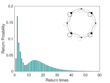
(a) MaxReturnEntropy chain on ring graph

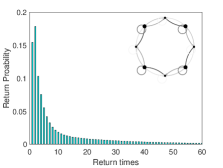
(b) MaxEntropyRate chain on ring graph

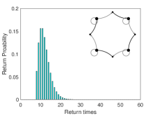
(c) MinKemeny chain on ring graph

Figure 2: Return time distributions of node $1$ (i.e., top node) on an $8$-node ring graph with stationary distribution $\bm{\pi}=[1/12,1/6,\dots,1/12,1/6]^{\top}$. Although the expectations of the first return time distributions in the figure are the same, the histogram is remarkably different for different chains. Specifically, for the nonreversible MaxRetrunEntropy chain, the distribution is bimodal and generates more entropy. The node size is proportional to the stationary distribution.

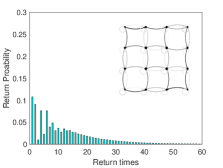
(a) MaxReturnEntropy chain on $4\times 4$ grid

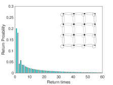
(b) MaxEntropyRate chain on $4\times 4$ grid

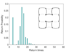
(c) MinKemeny chain on $4\times 4$ grid

Figure 3: Return time distributions of node $6$ (i.e., second node on the second row) on a $4\times 4$ grid with stationary distribution $\bm{\pi}$ proportional to the node degree and unitary travel times. The node size is proportional to the stationary distribution.

Chains on graphs with unitary travel times

Comparison: We consider $2$ simple undirected graphs and solve for the MaxReturnEntropy chain, the MaxEntropyRate chain and the MinKemeny chain for each case. We compare the return time entropy, the entropy rate, and the Kemeny constant of these chains in Table I. The stationary distribution of the ring graph is set to be $\bm{\pi}=[1/12,1/6,\dots,1/12,1/6]^{\top}$, and the stationary distribution of of grid is proportional to the degree of nodes. To evaluate the value of $\mathbb{J}(P)$, we set $\eta=10^{-2}$. From the table, we notice that the MaxReturnEntropy chain has the highest value of the return time entropy in both cases. It also has relatively good performance in terms of the entropy rate and the Kemeny constant, which indicates that the MaxReturnEntropy chain is potentially a good combination of speed (expected traversal time) and unpredictability. Furthermore, it is clear that (15), which characterizes the relationship between the entropy rate and the return time entropy, holds.

TABLE I: Comparison between different chains on different graphs

Graph	Markov chains	$\mathbb{J}(P)$	$\mathbb{H}_{\textup{rate}}(P)$	Kemeny constant
$8$-node ring	MaxReturnEntropy	2.4927	0.8698	10.0479
	MaxEntropyRate	2.3510	0.9883	19.5339
	MinKemeny	1.9641	0.4621	6.1667
$4$-by-$4$ grid	MaxReturnEntropy	3.6539	0.9491	16.3547
	MaxEntropyRate	3.2844	1.4021	30.8661
	MinKemeny	2.0990	0.2188	10.0938

Observations: In computing the MaxReturnEntropy chain, we observe some interesting properties of our problem. First, when solving Problem 2 by the gradient projection method with different initial conditions, we found different optimal solutions, and they have slightly different optimal values. This suggests that Problem 1 is unlikely to be a convex problem. Secondly, the global optimal solution to Problem 1 is possibly not unique in general. For instance, for an undirected ring graph with even number of nodes and certain stationary distribution, exchanging the probability of going right and that of going left for all nodes does not change the return time entropy. Thirdly, the optimal solution to Problem 1 is likely to be nonreversible because none of the approximate optimal solutions we have encountered are reversible. This again indicates that the MaxReturnEntropy chain is a good combination of unpredictability and speed. Fourth, even if we set the edge weight $\epsilon=0$, the MaxReturnEntropy chain is always irreducible.

Intuitions: In order to provide intuitions for the maximization of the return time entropy, we compare and plot the chains as well as the return time distribution of a same node on the $8$-node ring graph and the $4\times 4$ grid graph in Fig. 2 and Fig. 3, respectively. Since the stationary distribution is fixed and identical for all chains in each case, the expectations of the probability mass functions in each figure are the same. From the figures, we note that for the MaxReturnEntropy chain, the return time distribution is reshaped so that the distribution is more spread out and it is more difficult to predict the return time. In contrast, the return time distribution for the MinKemeny chain has a predictable pattern and the return time probability is constantly $0$ for some time intervals. Moreover, from the visualization of the chains, we notice that the MaxReturnEntropy chain has a net flow on the graph, which again indicates its nonreversibility.

MaxReturnEntropy and MinKemeny on a realistic map

In this part, we compare the MaxReturnEntropy chain with the MinKemeny chain on a realistic map with travel times. The problem data is taken from [3, Section 6.2]: a small area in San Francisco (SF) is modeled by a fully connected directed graph with $12$ nodes and by-car travel times on edges measured in seconds. The map is shown in Fig. 4. The importance of the a location (node) is characterized by the the number of crimes recorded at that place during a specific period, and the surveillance agent should visit the places with higher crime rate more often. The visit frequency is set to be $[\frac{133}{866},\frac{90}{866},\frac{89}{866},\frac{87}{866},\frac{83}{866},\frac{83}{866},\frac{74}{866},\frac{64}{866},\frac{48}{866},\frac{43}{866},\frac{38}{866},\frac{34}{866}]^{\top}$. For simplicity, we quantize the travel times by treating a minute as one unit of time, i.e., dividing the travel times by $60$ and round the result to the smallest integer that is larger than it, and by doing so, we have $w_{\max}=9$. The pairwise travel times are recorded in Table II.

Figure 4: San Francisco (SF) crime map from [3, Section 6.2].

TABLE II: The quantized pairwise by-car travel times on SF crime map

Location	A	B	C	D	E	F	G	H	I	J	K	L
A	1	3	3	5	4	6	3	5	7	4	6	6
B	3	1	5	4	2	4	4	5	5	3	5	5
C	3	5	1	7	6	8	3	4	9	4	8	7
D	6	4	7	1	5	6	4	7	5	6	6	7
E	4	3	6	5	1	3	5	5	6	3	4	4
F	6	4	8	5	3	1	6	7	3	6	2	3
G	2	5	3	5	6	7	1	5	7	5	7	8
H	3	5	2	7	6	7	3	1	9	3	7	5
I	8	6	9	4	6	4	6	9	1	8	5	7
J	4	3	4	6	3	5	5	3	7	1	5	3
K	6	4	8	6	4	2	6	6	4	5	1	3
L	6	4	6	6	3	3	6	4	5	3	2	1

First, we compare three key metrics of the MaxReturnEntropy chain and MinKemeny chain. The results are reported in Table III. It can be observed that the MaxReturnEntropy chain is much better than the MinKemeny chain regarding the return time entropy and the entropy rate. This better performance in terms of the unpredictability is obtained at the cost of being slower as indicated by the larger weighted Kemeny constant.

TABLE III: Comparison between different chains on SF crime map

Markov chains	$\mathbb{J}(P)$	$\mathbb{H}_{\textup{rate}}(P)$	Weighted Kemeny constant
MaxReturnEntropy	5.0078	1.7810	63.6007
MinKemeny	2.4678	0.6408	24.2824

We also plot the return time distribution of location A in Fig. 5. Apparently, the MaxReturnEntropy chain spreads the return time probabilities over the possible return times and it is hard to predict the exact time the surveillance agent comes back to the location. In contrast, the MinKemeny chain tries to achieve fast traversal on the graph and the return times distribute over a few intervals.

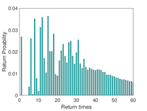
(a) MaxReturnEntropy chain on SF crime map

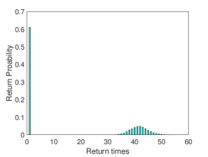
(b) MinKemeny chain on SF crime map

Figure 5: Return time distributions of location A on SF crime map. Note that the scales of the vertical axes are different in the two figures.

V-B Application to the Robotic Surveillance Problem

In this subsection, we provide simulation results in the application of robotic surveillance.

Setup: Consider the scenario where a single agent performs the surveillance task by moving randomly according to a Markov chain on the road map. The intruder is able to observe the local behaviors of the surveillance agent, e.g., presence/absence and duration between visits, and he/she plans and decides the time of attack so as to avoid being captured. It takes a certain amount of time for the intruder to complete an attack, which is called the attack duration of the intruder. A successful detection/capture happens when the surveillance agent and the intruder are at the same location and the intruder is attacking.

Intruder model (success probability maximizer with bounded patience): Consider a rational intruder that exploits the return time statistics of the Markov chains and chooses an optimal attack time so as to minimize the probability of being captured. The intruder picks a node $i$ to attack randomly according to the stationary distribution, and it collects and learns the probability distribution of node $i$’s first return time. Suppose the intruder and the surveillance agent are at the same node $i$ at the beginning and the attack duration of the intruder is $\tau$. If the intruder observes that the surveillance agent leaves the node and does not come back for $s$ periods, he/she can attack with the probability of being captured given by

$$\sum_{k=1}^{\tau}\mathbb{P}(T_{ii}=s+k\,|\,T_{ii}>s).$$ (33)

Mathematically speaking, (33) is the conditional cumulative return probability for the surveillance agent. Specifically for $s=0$, (33) is the capture probability when the intruder attacks immediately after the agent leaves the node. Then, the optimal time of attack $s_{i}$ for the intruder is given by

$$s_{i}=\operatorname*{argmin}_{0\leq s\leq S_{i}}\{\sum_{k=1}^{\tau}\mathbb{P}(T_{ii}=s+k\,|\,T_{ii}>s)\}.$$ (34)

The reason there is an upper bound $S_{i}$ on $s$ is that the event $T_{ii}>s$ happens with very low probability when $s$ is large, and the intruder may be unwilling to wait for such an event to happen. Let $\delta\in(0,1)$ be the degree of impatience of the intruder, then $S_{i}$ can be chosen as the minimal positive integer such that the following holds,

$$\mathbb{P}(T_{ii}\geq S_{i})\leq\delta,$$

where a smaller $\delta$ implies a larger $S_{i}$ and a more patient intruder. In other words, when $\delta$ is small, the intruder is willing to wait for a rare event to happen. Note that the value of $S_{i}$ is also dependent on the node $i$ that the intruder chooses to attack, and thus the argmin in (34) is over different ranges when the intruder attacks different nodes. In summary, the intruder is dictated by two parameters: the attack duration $\tau$ and the degree of impatience $\delta$, and the strategy for the intruder is as follows: waits until the event that the surveillance agent leaves and does not come back for the first $s_{i}$ steps happens, then attacks immediately.

From the surveillance point of view, the probability of capturing the rational intruder when he/she attacks node $i$ is

$$\mathbb{P}_{i}(\text{Capture})=\sum_{k=1}^{\tau}\mathbb{P}(T_{ii}=s_{i}+k\,|\,T_{ii}>s_{i}),$$

and the performance of the Markov chains can be evaluated by the total probability of capture as follows

$$\mathbb{P}(\text{Capture})=\sum_{i=1}^{n}\pi_{i}\mathbb{P}_{i}(\text{Capture}).$$ (35)

Simulation results: Designing an optimal defense mechanism for the rational intruder is an interesting yet challenging problem in its own. Instead, we use the MaxReturnEntropy chain as a heuristic solution and compare its performance with other chains. In the following, we consider two types of graphs: the grid graph and the SF crime map. The degree of impatience of the intruder is set to be $\eta=0.1$ in this part.

We first consider a $4\times 4$ grid and plot the probability of capture defined by (35) for the chains in comparison in Fig. 6. It can be observed that, when defending against the rational intruder described above, the MaxReturnEntropy chain outperforms all other chains when the attack duration of the intruder is small or moderate. The unpredictability in the return time prevents the rational intruder from taking advantage of the visit statistics learned from the observations. The MinKemeny chain, which emphasizes a faster traversal, has a hard time capturing the intruder when the attack duration of the intruder is small. This is because the agent moves in a relatively more predictable way, and the return time statistics may have a pattern that could be exploited. The MaxEntropyRate chain has the in-between performance.

Figure 6: Performance of different chains on a $4\times 4$ grid.

For the SF crime map, we use the same problem data as described in Subsection V-A. Since the MaxEntropyRate chain does not generalize to the case when there are travel times, we compare the performance of the MaxReturnEntropy chain and the MinKemny chain. Again, The MaxReturnEntropy chain outperforms the MinKemeny chain when the attack duration of the intruder is relatively small.

Figure 7: Performance of different chains on the SF crime map.

Summary: The simulation results presented in this subsection demonstrate that the MaxReturnEntropy chain is an effective strategy against the intruder with reasonable amount of knowledge and level of intelligence, particularly when the attack duration of the intruder is small or moderate. With the property of both unpredictability and speed, the MaxReturnEntropy chain should also work well in a much more broader range of scenarios.

VI Conclusion

In this paper, we proposed and optimized a new metric that quantifies the unpredictability of Markov chains over a directed strongly connected graph with travel times, i.e., the return time entropy. We characterized the return time probabilities and showed that optimizing the return time entropy is a well-posed problem. For the case of unitary travel times, we established an upper bound for the return time entropy by using the maximum entropy principle and obtained an analytic solution for the complete graph. We connected the return time entropy with the well-known entropy rate of Markov chains and showed that the return time entropy is lower bounded by the entropy rate and upper bounded by $n$ times the entropy rate. In order to solve the optimization problem numerically, we approximated the return time entropy as well as a practically useful conditional return time entropy by the truncated return time entropy. We derived the gradient of the truncated return time entropy and proposed to solve the problem by the gradient projection method. We applied our results to the robotic surveillance problem and found that the chain with maximum return time entropy is a good trade-off between speed and unpredictability, and it performs better than several existing chains against a rational intruder.

A number of problems are still open. First of all, a simple closed-form expression for the return time entropy would enable us to establish more properties of the objective function and thus make the optimization problem more tractable. Second, it is interesting to design a best Markov chain directly that defends against the intruder model proposed in this paper. Third, how to generalize the results to the case of multiple robots remains to be investigated. Fourth, we believe there are more application scenarios for Markov chains where the return time entropy is an appropriate quantity to optimize.

References

• [1] B. Açıkmeşe and S. D. Bayard. Markov chain approach to probabilistic guidance for swarms of autonomous agents. Asian Journal of Control, 17(4):1105–1124, 2015. doi:10.1002/asjc.982.
• [2] N. Agmon, S. Kraus, and G. A. Kaminka. Multi-robot perimeter patrol in adversarial settings. In IEEE Int. Conf. on Robotics and Automation, pages 2339–2345, Pasadena, USA, May 2008. doi:10.1109/ROBOT.2008.4543563.
• [3] S. Alamdari, E. Fata, and S. L. Smith. Persistent monitoring in discrete environments: Minimizing the maximum weighted latency between observations. International Journal of Robotics Research, 33(1):138–154, 2014. doi:10.1177/0278364913504011.
• [4] E. Arvelo and N. C. Martins. Maximizing the set of recurrent states of an MDP subject to convex constraints. Automatica, 50(3):994–998, 2014. doi:10.1016/j.automatica.2014.01.002.
• [5] A. B. Asghar and S. L. Smith. Stochastic patrolling in adversarial settings. In American Control Conference, pages 6435–6440, Boston, USA, July 2016. doi:10.1109/ACC.2016.7526682.
• [6] S. Bandyopadhyay, S. J. Chung, and F. Y. Hadaegh. Probabilistic and distributed control of a large-scale swarm of autonomous agents. IEEE Transactions on Robotics, 33(5):1103–1123, 2017. doi:10.1109/TRO.2017.2705044.
• [7] D. P. Bertsekas. Nonlinear Programming. Athena Scientific, 3 edition, 2016.
• [8] S. Boyd and L. Vandenberghe. Convex Optimization. Cambridge University Press, 2004.
• [9] G. Cannata and A. Sgorbissa. A minimalist algorithm for multirobot continuous coverage. IEEE Transactions on Robotics, 27(2):297–312, 2011. doi:10.1109/TRO.2011.2104510.
• [10] Y. Chen, T. Georgiou, M. Pavon, and A. Tannenbaum. Robust transport over networks. IEEE Transactions on Automatic Control, 62(9):4675–4682, 2017. doi:10.1109/TAC.2016.2626796.
• [11] M. H. A. Davis and R. B. Vinter. Stochastic Modelling and Control. Springer, 1985. doi:10.1007/978-94-009-4828-0.
• [12] L. Ekroot and T. M. Cover. The entropy of Markov trajectories. IEEE Transactions on Information Theory, 39:1418–1421, 1993. doi:10.1109/18.243461.
• [13] M. George, S. Jafarpour, and F. Bullo. Markov chains with maximum entropy for robotic surveillance. IEEE Transactions on Automatic Control, May 2018. To appear. URL: http://motion.me.ucsb.edu/pdf/2017b-gjb.pdf.
• [14] J. Grace and J. Baillieul. Stochastic strategies for autonomous robotic surveillance. In IEEE Conf. on Decision and Control and European Control Conference, pages 2200–2205, Seville, Spain, December 2005. doi:10.1109/CDC.2005.1582488.
• [15] S. Guiasu and A. Shenitzer. The principle of maximum entropy. The Mathematical Intelligencer, 7(1):42–48, 1985. doi:10.1007/BF03023004.
• [16] A. Hmamed and E. Tissir. Further results on the stability of discrete-time matrix polynomials. International Journal of Systems Science, 29(8):819–821, 1998. doi:10.1080/00207729808929574.
• [17] J. G. Kemeny and J. L. Snell. Finite Markov Chains. Springer, 1976.
• [18] C. D. Meyer. Matrix Analysis and Applied Linear Algebra. SIAM, 2001.
• [19] N. Noori, A. Renzaglia, J. V. Hook, and V. Isler. Constrained probabilistic search for a one-dimensional random walker. IEEE Transactions on Robotics, 32(2):261–274, 2016. doi:10.1109/TRO.2015.2513751.
• [20] J. R. Norris. Markov Chains. Cambridge University Press, 1997. doi:10.1017/CBO9780511810633.
• [21] R. Patel, P. Agharkar, and F. Bullo. Robotic surveillance and Markov chains with minimal weighted Kemeny constant. IEEE Transactions on Automatic Control, 60(12):3156–3167, 2015. doi:10.1109/TAC.2015.2426317.
• [22] R. Patel, A. Carron, and F. Bullo. The hitting time of multiple random walks. SIAM Journal on Matrix Analysis and Applications, 37(3):933–954, 2016. doi:10.1137/15M1010737.
• [23] W. Rudin. Principles of Mathematical Analysis. International Series in Pure and Applied Mathematics. McGraw-Hill, 3 edition, 1976.
• [24] K. Srivastava, D. M. Stipanovic̀, and M. W. Spong. On a stochastic robotic surveillance problem. In IEEE Conf. on Decision and Control, pages 8567–8574, Shanghai, China, December 2009. doi:10.1109/CDC.2009.5400569.
• [25] H. Xu, B. Ford, F. Fang, B. Dilkina, A. Plumptre, M. Tambe, M. Driciru, F. Wanyama, A. Rwetsiba, M. Nsubaga, and J. Mabonga. Optimal patrol planning for green security games with black-box attackers. In International Conference on Decision and Game Theory for Security, pages 458–477. Springer, 2017. doi:10.1007/978-3-319-68711-7_24.
• [26] J. Yu, S. Karaman, and D. Rus. Persistent monitoring of events with stochastic arrivals at multiple stations. IEEE Transactions on Robotics, 31(3):521–535, 2015. doi:10.1109/TRO.2015.2409453.