Inverse Optimal Control from Incomplete Trajectory Observations

Abstract

This article develops a methodology that enables learning an objective function of an optimal control system from incomplete trajectory observations. The objective function is assumed to be a weighted sum of features (or basis functions) with unknown weights, and the observed data is a segment of a trajectory of system states and inputs. The proposed technique introduces the concept of the recovery matrix to establish the relationship between any available segment of the trajectory and the weights of given candidate features. The rank of the recovery matrix indicates whether a subset of relevant features can be found among the candidate features and the corresponding weights can be learned from the segment data. The recovery matrix can be obtained iteratively and its rank non-decreasing property shows that additional observations may contribute to the objective learning. Based on the recovery matrix, a method for using incomplete trajectory observations to learn the weights of selected features is established, and an incremental inverse optimal control algorithm is developed by automatically finding the minimal required observation. The effectiveness of the proposed method is demonstrated on a linear quadratic regulator system and a simulated robot manipulator.

1 Introduction

Inverse optimal control (IOC), also known as inverse reinforcement learning, solves a problem of finding an objective (e.g., cost or reward) function to explain behavioral observations of an optimal control system (Kalman, 1964; Ng and Russell, 2000). Successful applications of IOC techniques are broad, including imitation learning (Abbeel et al., 2010; Kolter et al., 2008), where a learner mimics an expert by inferring an objective function from the expert’s demonstrations, autonomous driving (Kuderer et al., 2015), where human driving preference is learned and transferred to a vehicle controller, human-robot shared systems (Mainprice et al., 2015, 2016), where the intentionality of a human partner is estimated to enable motion prediction and smooth coordination, and human motion analysis (Jin et al., 2019; Lin et al., 2016), where principles of human motor control are investigated.

The most common strategy used in IOC is to parametrize an unknown objective function as a weighted sum of relevant features (or basis functions) with unknown weights (Ng and Russell, 2000; Abbeel and Ng, 2004; Ratliff et al., 2006; Ziebart et al., 2008; Mombaur et al., 2010; Englert et al., 2017). Different approaches have been developed to estimate the weights of the features given a full observation of the system’s optimal trajectory over a complete motion horizon. These methods cannot deal with the case when only incomplete trajectory observations are available, that is, only a portion/segment of the system’s trajectory within a small time interval of the horizon is available. A method capable of learning objective functions from incomplete trajectory data will be beneficial for multiple reasons: first, a full observation of the system’s trajectory over a complete time horizon may not be accessible due to limited sensing capabilities, sensor failures, occlusions, etc; second, the computational cost of existing IOC techniques based on full trajectory data may be large; and third, learning objective functions from incomplete trajectory observations may help to address some other challenging problems such as learning time-varying objective functions (Jin et al., 2019), online motion prediction (Pérez-D’Arpino and Shah, 2015), and learning from human corrections (Bajcsy et al., 2018). Under these motivations, this article aims to develop a technique to enable learning an objective function only from incomplete trajectory observations.

1.1 Related Work

Existing IOC methods can be categorized based on whether the forward optimal control problem needs to be computed within the learning process. The first category of existing works is based on a nested architecture, where the feature weights are updated in an outer loop while the corresponding optimal control system is solved in an inner loop. Different methods of this type focus on different strategies to update the feature weights in the outer layer. Representative methods include (Abbeel and Ng, 2004), where the feature weights are updated towards matching the feature values of the reproduced optimal trajectories with the demonstrations, (Ratliff et al., 2006), where the feature weights are solved by maximizing the margin between the objective function value of the observed trajectories and the value of any simulated optimal trajectories, and (Ziebart et al., 2008), where the feature weights are optimized such that the probability distribution of system’s trajectories maximizes the entropy while matching the empirical feature values of demonstrations. These nested IOC methods have been successfully applied to humanoid locomotion (Park and Levine, 2013), autonomous vehicles (Kuderer et al., 2015), robot navigation (Vasquez et al., 2014), learning from human corrections (Bajcsy et al., 2017; Jin et al., 2020), etc. In (Mombaur et al., 2010), the weights are learned by minimizing the deviation of the reproduced optimal trajectory from the observed one; the similar methods are applied to studying human walking (Clever et al., 2016) and arm motion (Berret et al., 2011).

A drawback of the nested IOC methods is the need to solve optimal control problems repeatedly in the inner loop, thus those methods usually suffer from huge computational cost. This motivates the second line of IOC methods, which seek to directly solve for the unknown feature weights. A key idea used in these methods is to establish optimality conditions which the observed optimal data must satisfy. For example, in (Keshavarz et al., 2011), the Karush-Kuhn-Tucker (KKT) (Boyd and Vandenberghe, 2004) optimality conditions are established, based on which the feature weights are then solved by minimizing a loss that quantifies the violation of such conditions by the observed data. In (Puydupin-Jamin et al., 2012), the authors apply such the KKT-based method to solve IOC problems and study the objective function underlying human locomotion. In (Johnson et al., 2013), the Pontryagin’s Minimum Principle (Pontryagin et al., 1962) is utilized to formulate a residual optimization over the unknown weights. These methods have been successfully applied to the locomotion analysis (Aghasadeghi and Bretl, 2014; Puydupin-Jamin et al., 2012), walking path generation (Papadopoulos et al., 2016), human motion segmentation (Lin et al., 2016; Jin et al., 2019), etc. In (Englert et al., 2017), the authors propose an inverse KKT method to enable a robot to learn manipulation tasks. Recently, along this direction, the recoverability for IOC problems has been investigated. For example, when an optimal control system remains at an equilibrium point, although its trajectory still satisfies the optimality conditions, it is uninformative for learning the objective function. This issue is discussed in (Molloy et al., 2016, 2018), where a sufficient condition for recovering weights from full trajectory observations is proposed.

Existing IOC techniques discussed above require a full observation of a system trajectory, that is, optimal trajectory data of the system states and inputs over a complete motion horizon. To our best knowledge, the IOC problems based on incomplete trajectory observations are rarely investigated. By an incomplete trajectory observation, we mean that the observed data is a segment or portion of the system trajectory within a small time interval of the horizon. We consider the objective learning using incomplete trajectory data mainly due to the following motivations. First, in certain practical cases, for example, due to limited sensing, sensors’ failure, or occlusions, a full observation of system’s trajectory data may not be available. Second, although direct IOC methods improve the computation efficiency compared to the nested counterparts, the computational cost is still significant especially when handling complex systems with high-dimensional action/state space and long time horizons. Third, successfully learning objective functions only using incomplete trajectory data would potentially benefit for addressing many challenging problems such as identifying time-varying objective functions (Jin et al., 2019), learning from human corrections (Bajcsy et al., 2018), online long-term motion prediction (Mainprice et al., 2016), etc.

1.2 Contributions

This article develops a methodology to learn an objective function of an optimal control system using incomplete trajectory observations. The proposed key concept to achieve this goal is the recovery matrix, which is defined on any segment data of the system trajectory and a given candidate feature set. We show that learning of the objective function is related to the rank and kernel properties of the recovery matrix. Different from existing methods, the recovery matrix also captures the unseen future information in addition to the available data by an unknown costate variable, which is jointly estimated along with the unknown feature weights. By investigating the properties of the recovery matrix, the following insights to solving IOC problems are enabled:

• The rank of the recovery matrix indicates whether an observation of incomplete trajectory data is sufficient for learning the feature weights;

• Additional observation data can contribute to learning the unknown objective function, or at least not degrade the learning; and irrelevant features can be identified.

• The IOC can be solved by incrementally incorporating the observation of each data point along the trajectory.

Based on the recovery matrix, an IOC approach based on incomplete trajectory observations is established, and an incremental IOC algorithm is developed by automatically finding the minimal required observation.

The structure of this article is as follows. Section 2 states the problem. Section 3 develops the recovery matrix and its properties. Section 4 presents the IOC method and algorithm using incomplete trajectory observations. Section 5 conducts numerical experiments, and Section 6 draws conclusions.

Notation

The column operator ${\rm col\;}\{\boldsymbol{x}_{1},...,\boldsymbol{x}_{k}\}$ stacks its arguments into a column. $\boldsymbol{x}_{k_{1}:k_{2}}$ means a column stack of $\boldsymbol{x}$ indexed from $k_{1}$ to $k_{2}$ ($k_{1}\leq k_{2}$), that is, $\boldsymbol{x}_{k_{1}:k_{2}}={\rm col\;}\{\boldsymbol{x}_{k_{1}},...\boldsymbol{x}_{k_{2}}\}$. $\boldsymbol{A}$ (bold) denotes a block matrix. Given a vector function $\boldsymbol{f}(\boldsymbol{x})$ and a constant $\boldsymbol{x}^{*}$, $\frac{\partial\boldsymbol{f}}{\partial\boldsymbol{x}^{*}}$ denotes the Jacobian matrix with respect to $\boldsymbol{x}$ evaluated at $\boldsymbol{x}^{*}$. The zero matrix and vector are written as $\boldsymbol{0}$, and the identity matrix as ${\boldsymbol{I}}$, both with appropriate dimensions. $\boldsymbol{A}^{\prime}$ is the transpose of matrix $\boldsymbol{A}$. $\sigma_{i}(\boldsymbol{A})$ denotes the $i$th smallest singular value of matrix $\boldsymbol{A}$, e.g., $\sigma_{1}(\boldsymbol{A})$ is the smallest singular value. $\ker\boldsymbol{A}$ denotes the kernel of matrix $\boldsymbol{A}$.

2 Problem Formulation

Consider an optimal control system with the following discrete-time dynamics and initial condition:

$$\boldsymbol{x}_{k+1}=\boldsymbol{\boldsymbol{f}}(\boldsymbol{x}_{k},\boldsymbol{u}_{k}),\quad\boldsymbol{x}_{0}\in\mathbb{R}^{n},\\$$ (1)

where the vector function $\boldsymbol{f}:\mathbb{R}^{n}\times\mathbb{R}^{m}\mapsto\mathbb{R}^{n}$ is differentiable; $\boldsymbol{x}_{k}\in\mathbb{R}^{n}$ is the system state; $\boldsymbol{u}_{k}\in\mathbb{R}^{m}$ is the control input; and $k=0,1,\cdots$ is the time step. Suppose a trajectory of states and inputs over a horizon $T$,

$$\boldsymbol{\xi}=\{\boldsymbol{\xi}_{k}:k=0,1,...,T\}\,\,\text{ with }\,\,\,\boldsymbol{\xi}_{k}{=}(\boldsymbol{x}^{*}_{k},\,\boldsymbol{u}^{*}_{k}),$$ (2)

(locally) minimizes a cost function

$$J(\boldsymbol{\xi})=\sum\nolimits_{{k=0}}^{T}{{\boldsymbol{\omega}}^{\prime}\boldsymbol{\phi}}^{*}(\boldsymbol{x}_{k},\boldsymbol{u}_{k}),$$ (3)

where ${\boldsymbol{\omega}}^{\prime}\boldsymbol{\phi}^{*}(\cdot,\cdot)$ is the running cost. Here $\boldsymbol{\phi}:\mathbb{R}^{n}\times\mathbb{R}^{m}\mapsto\mathbb{R}^{s}$ is called a relevant feature vector and defined as a column of a relevant feature set

$$\mathcal{F}^{*}=\{\phi_{1}^{*},\phi_{2}^{*},\cdots,\phi_{s}^{*}\},$$ (4)

that is, $\boldsymbol{\phi}^{*}={\rm col\;}{\mathcal{F}}^{*}$, with $\phi_{i}^{*}$ being the $i$th feature for the running cost, and $\boldsymbol{\omega}\in\mathbb{R}^{s}$ is called the weight vector, with the $i$th entry $\omega_{i}$ corresponding to $\phi_{i}^{*}$. This type of weighted-feature objective function is commonly used in objective learning problems (Abbeel and Ng, 2004; Molloy et al., 2018; Ziebart et al., 2008), and has been successfully applied in a wide range of real-world applications (Englert et al., 2017; Kuderer et al., 2015; Lin et al., 2016; Bajcsy et al., 2018). The dynamics (1) and cost function (3) can represent different optimal control settings as follows. (I) Finite-horizon free-end optimal control: the finite horizon $T$ is given but the final state $\boldsymbol{x}_{T+1}$ is free, i.e., no constraint on $\boldsymbol{x}_{T+1}$; (II) finite-horizon fixed-end optimal control: both the finite horizon $T$ and the final state $\boldsymbol{x}_{T+1}=\boldsymbol{x}_{\text{goal}}$ are given; and (III) infinite-horizon optimal control: $T=\infty$. Besides, one can consider the finite-horizon optimal control, where the final state $\boldsymbol{x}_{T+1}$ is penalized using a final cost term added to (3), and this case can be viewed as an extension similar to (II). In our following expositions, we only focus on the first three settings.

In inverse optimal control (IOC) problems, one is given a relevant feature set $\mathcal{F}^{*}$, the goal is to obtain an estimate of the weights $\boldsymbol{\omega}$ corresponding to these features from observations of $\boldsymbol{\xi}$. Note that $\boldsymbol{\omega}$ can only be determined up to a non-zero scaling factor (Molloy et al., 2018; Keshavarz et al., 2011), because any $c\boldsymbol{\omega}$ with $c>0$ will lead to the same trajectory $\boldsymbol{\xi}$. Hence we say an estimate $\hat{\boldsymbol{\omega}}$ is a successful estimate of $\boldsymbol{\omega}$ if $\hat{\boldsymbol{\omega}}=c\boldsymbol{\omega}$ with $c\neq 0$, and the specific $c>0$ can be determined by normalization (Keshavarz et al., 2011; Englert et al., 2017).

We have noted that existing IOC methods typically assume that the full trajectory data $\boldsymbol{\xi}$ is available. Violation of this assumption will lead to a failure of existing approaches, as we will demonstrate in the numerical evaluation in Section 5. In this article, we aim to address this challenge by developing a technique to estimate $\boldsymbol{\omega}$ only using incomplete trajectory data. Specifically, given a relevant feature set $\mathcal{F}^{*}$, the goal of this paper is to achieve a successful estimate $\hat{\boldsymbol{\omega}}=c\boldsymbol{\omega}$ using an incomplete trajectory observation

$$\boldsymbol{\xi}_{{t:t+l}}=\{\boldsymbol{\xi}_{k}:t\leq k\leq{t+l}\}\subseteq\boldsymbol{\xi},$$ (5)

which is a segment of $\boldsymbol{\xi}$ within the time interval $[t,{t+l}]\subseteq[0,T]$. Here, $t$ is called the observation starting time and $l=1,2,\cdots$ called the observation length, with $0\leq t<{t+l}\leq T$. Moreover, for any observation starting time $t$, we aim to efficiently find the minimal required observation, that is, $l_{\min}$, to achieve a successful estimate of $\boldsymbol{\omega}$. Note that in the above problem setting, we only know that the data $\boldsymbol{\xi}_{t:{t+l}}$ is a segment of a system trajectory $\boldsymbol{\xi}$; we do not know the value of $t$ (i.e., the observation starting time relative to the start of the trajectory), and do not require knowledge of any other information about $\boldsymbol{\xi}$ such as the time horizon $T$ or which type of optimal control problem $\boldsymbol{\xi}$ is a solution to.

3 The Recovery Matrix

In this section, we introduce the key concept of the recovery matrix and show its relation to IOC process. Some properties of the recovery matrix are investigated to provide insights to IOC process. Connections between the recovery matrix and existing methods is also discussed. The implementation of the recovery matrix is finally presented.

3.1 Definition of the Recovery Matrix

We first present the definition of the recovery matrix, then show its relation to the IOC problem solution, which is also the motivation of the recovery matrix.

Definition 1.

Let a segment of the trajectory, $\boldsymbol{\xi}_{t:{t+l}}\subseteq\boldsymbol{\xi}$ in (5), and a candidate feature set $\mathcal{F}=\{\phi_{1},\phi_{2},\cdots,\phi_{r}\}$ be given. Let $\boldsymbol{\phi}={\rm col\;}\mathcal{F}$. Then the recovery matrix, denoted by $\boldsymbol{H}(t,l)$, is defined as:

$$\boldsymbol{H}(t,l)=\begin{bmatrix}\boldsymbol{H}_{1}(t,l)&\boldsymbol{H}_{2}(t,l)\end{bmatrix}\in\mathbb{R}^{ml\times(r+n)},$$ (6)

with

$$\boldsymbol{H}_{1}(t,l) =\boldsymbol{F}_{u}(t,l)\boldsymbol{F}^{-1}_{x}(t,l)\boldsymbol{\Phi}_{x}(t,l)+\boldsymbol{\Phi}_{u}(t,l),$$ (7)

$$\boldsymbol{H}_{2}(t,l) =\boldsymbol{F}_{u}(t,l)\boldsymbol{F}_{x}^{-1}(t,l)\boldsymbol{V}(t,l).$$ (8)

Here, $\boldsymbol{F}_{x}(t,l)$, $\boldsymbol{F}_{u}(t,l)$, $\boldsymbol{\Phi}_{x}(t,l)$, $\boldsymbol{\Phi}_{u}(t,l)$ and $\boldsymbol{V}(t,l)$ are defined as

$$\boldsymbol{F}_{x}(t,l) =\begin{bmatrix}\boldsymbol{I}&\,\,\frac{-\partial\boldsymbol{f}^{\prime}}{\partial\boldsymbol{x}^{*}_{{t+1}}}&&\\ \boldsymbol{0}&\boldsymbol{I}&\ddots&\\ &&\ddots&\,\,\,\,\,\frac{-\partial\boldsymbol{f}^{\prime}}{\partial\boldsymbol{x}^{*}_{{t\text{+}l\text{-}1}}}\\[7.0pt] &&&\boldsymbol{I}\\ \end{bmatrix}\in\mathbb{R}^{nl\times nl},$$ (9)

$$\boldsymbol{F}_{u}(t,l) =\begin{bmatrix}\frac{\partial\boldsymbol{f}^{\prime}}{\partial\boldsymbol{u}^{*}_{t}}&&&\\ &\frac{\partial\boldsymbol{f}^{\prime}}{\partial\boldsymbol{u}^{*}_{t+1}}&&\\ &&\ddots&\\ &&&\frac{\partial\boldsymbol{f}^{\prime}}{\partial\boldsymbol{u}^{*}_{t\text{+}l\text{-}1}}\end{bmatrix}\in\mathbb{R}^{ml\times nl},$$ (10)

$$\boldsymbol{\Phi}_{x}(t,l) =\begin{bmatrix}\frac{\partial\boldsymbol{\phi}}{\partial\boldsymbol{x}^{*}_{{t+1}}}&\frac{\partial\boldsymbol{\phi}}{\partial\boldsymbol{x}^{*}_{{t\text{+}2}}}&\cdots&\frac{\partial\boldsymbol{\phi}}{\partial\boldsymbol{x}^{*}_{{t\text{+}l}}}\end{bmatrix}^{\prime}\in\mathbb{R}^{nl\times r},$$ (11)

$$\boldsymbol{\Phi}_{u}(t,l) =\begin{bmatrix}\frac{\partial\boldsymbol{\phi}}{\partial\boldsymbol{u}^{*}_{t}}&\frac{\partial\boldsymbol{\phi}}{\partial\boldsymbol{u}^{*}_{t+1}}&\cdots&\frac{\partial\boldsymbol{\phi}}{\partial\boldsymbol{u}^{*}_{t\text{+}l\text{-}1}}\end{bmatrix}^{\prime}\in\mathbb{R}^{ml\times r},$$ (12)

$$\boldsymbol{V}(t,l) =\begin{bmatrix}\boldsymbol{0}&\frac{\partial\boldsymbol{f}}{\partial\boldsymbol{x}^{*}_{{t\text{+}l}}}\end{bmatrix}^{\prime}\in\mathbb{R}^{nl\times n},$$ (13)

respectively.

Before showing a relationship between the above recovery matrix and IOC, we impose the following assumption on the given candidate feature set $\mathcal{F}$ in Definition 1.

Assumption 1.

In Definition 1, the candidate feature set $\mathcal{F}$ contains as a subset the relevant features $\mathcal{F^{*}}$ in (4), i.e., $\mathcal{F^{*}}\subseteq\mathcal{F}$.

Assumption 1 requires that the relevant features $\mathcal{F^{*}}$ in (4) are contained by the given candidate feature set $\mathcal{F}$, which means that $\mathcal{F}$ also allows for including additional features that are irrelevant to the optimal control system. Although restrictive for choice of features, this assumption is likely to be fulfilled in implementation by providing a larger set including many features when the knowledge of exact relevant features is not available. Under Assumption 1, without loss of generality, we let

$$\mathcal{F}=\{\phi_{1}^{*},\phi_{2}^{*},\cdots,\phi_{s}^{*},\tilde{\phi}_{s+1},\cdots,\tilde{\phi}_{r}\},$$ (14)

that is, the first $s$ elements are from $\mathcal{F}^{*}$ in (4). Then we have

$$\boldsymbol{\phi}(\boldsymbol{x},\boldsymbol{u})={\rm col\;}{\mathcal{F}}=\begin{bmatrix}\boldsymbol{\phi}^{*}(\boldsymbol{x},\boldsymbol{u})\\ \tilde{\boldsymbol{\phi}}(\boldsymbol{x},\boldsymbol{u})\end{bmatrix}\in\mathbb{R}^{r},$$ (15)

where $\boldsymbol{\phi}^{*}\in\mathbb{R}^{s}$ are the relevant feature vector in (3) while $\tilde{\boldsymbol{\phi}}\in\mathbb{R}^{(r-s)}$ corresponds to the features that are not in $\mathcal{F^{*}}$. We define a weight vector

$$\bar{\boldsymbol{\omega}}={\rm col\;}\{\boldsymbol{\omega},\boldsymbol{0}\}\in\mathbb{R}^{r}$$ (16)

corresponding to (15), where $\boldsymbol{\omega}$ are the weights in (3) for $\boldsymbol{\phi}^{*}$. Based on (3), we can say that the system’s optimal trajectory $\boldsymbol{\xi}$ in (2) also (locally) minimize the cost function of

$${J}(\boldsymbol{\xi})=\sum_{{k=0}}^{T}\bar{\boldsymbol{\omega}}^{\prime}\boldsymbol{\phi}(\boldsymbol{x}_{k},\boldsymbol{u}_{k}),$$ (17)

with the dynamics and initial condition in (1). Next, we will distinguish the three optimal control settings, as described in the problem formulation, and then establish the relationship between the recovery matrix and the IOC problem solution.

Case I: Finite-Horizon Free-End Optimal Control.

We first consider the optimal control setting with finite horizon $T$ and free final state $\boldsymbol{x}_{T+1}$. In this case, given the cost function (17) and the dynamics constraint (1), one can define the following Lagrangian:

$${L}={J}(\boldsymbol{\xi}){+}\sum_{k=0}^{T}\boldsymbol{\lambda}_{k{+}1}^{\prime}\big{(}\boldsymbol{f}(\boldsymbol{x}_{k},\boldsymbol{u}_{k})-\boldsymbol{x}_{k{+}1}\big{)},$$ (18)

where $\boldsymbol{\lambda}_{k+1}\in{\mathbb{R}^{n}}$, $k=0,1,\dots,{T}$, is Lagrange multipliers. According to the Karush-Kuhn-Tucker (KKT) optimality conditions (Boyd and Vandenberghe, 2004), there exist multipliers $\boldsymbol{\lambda}^{*}_{1:T+1}={\rm col\;}\{\boldsymbol{\lambda}_{1}^{*},\boldsymbol{\lambda}_{2}^{*},...,\boldsymbol{\lambda}_{T}^{*},\boldsymbol{\lambda}_{T+1}^{*}\}$, also referred to as costates, such that the optimal trajectory $\boldsymbol{\xi}$ must satisfy the following conditions

$$\frac{\partial{L}}{\partial\boldsymbol{x}^{*}_{{1:T+1}}} =\boldsymbol{0},$$ (19a)

$$\frac{\partial{L}}{\partial\boldsymbol{u}^{*}_{{0:T}}} =\boldsymbol{0}.$$ (19b)

Based on the definitions in (9)-(13), the equations in (19a) and (19b) can be written as

$$-\boldsymbol{F}_{x}({0,T})\boldsymbol{\lambda}_{{1:T}}^{*}{+}\boldsymbol{\Phi}_{x}({0,T})\bar{\boldsymbol{\omega}} =\boldsymbol{0}=-\boldsymbol{V}({0,T})\boldsymbol{\lambda}^{*}_{{T+1}},$$ (20a)

$$\boldsymbol{F}_{u}({0,T})\boldsymbol{\lambda}_{{1:T}}^{*}{+}\boldsymbol{\Phi}_{u}({0,T})\bar{\boldsymbol{\omega}} =\boldsymbol{0},$$ (20b)

respectively, where in (20a), $\boldsymbol{\lambda}^{*}_{T+1}=\boldsymbol{0}$ directly results from extending (19a) at the final state $\boldsymbol{x}_{T+1}$. The optimality equations in (20) are established for full optimal trajectory $\boldsymbol{\xi}$. Given any segment of the trajectory, say $\boldsymbol{\xi}_{{t:t+l}}\subseteq\boldsymbol{\xi}$ in (5), the following equations can be obtained by partitioning (20a) and (20b) in rows,

$$-\boldsymbol{F}_{x}(t,l)\boldsymbol{\lambda}_{{t+1:t+l}}^{*}+\boldsymbol{\Phi}_{x}(t,l)\bar{\boldsymbol{\omega}} =-\boldsymbol{V}(t,l)\boldsymbol{\lambda}_{{t+l+1}}^{*},$$ (21a)

$$\boldsymbol{F}_{u}(t,l)\boldsymbol{\lambda}_{{t+1:t+l}}^{*}+\boldsymbol{\Phi}_{u}(t,l)\bar{\boldsymbol{\omega}} =\boldsymbol{0},$$ (21b)

respectively. For the above (21), we note that when $\boldsymbol{\xi}_{t:t+l}=\boldsymbol{\xi}_{0:T}$, i.e., when the observation is the full trajectory data $\boldsymbol{\xi}$, (21) will become (20). Thus, a full trajectory observation can be viewed as a special case of an incomplete trajectory observation, and we will further discuss this in Section 3.3.

Case II: Finite-Horizon Fixed-End Optimal Control.

We next consider the optimal control setting with a finite horizon $T$ and a given fixed final state $\boldsymbol{x}_{T+1}=\boldsymbol{x}_{\text{goal}}$. Given the cost function (17), the dynamics (1), and the final state constraint $\boldsymbol{x}_{T+1}=\boldsymbol{x}_{\text{goal}}$, one can define the following Lagrangian:

$${L}{=}{J}(\boldsymbol{\xi}){+}\sum_{k=0}^{T}\boldsymbol{\lambda}_{k\text{+}1}^{\prime}\big{(}\boldsymbol{f}(\boldsymbol{x}_{k},\boldsymbol{u}_{k}){-}\boldsymbol{x}_{k\text{+}1}\big{)}{+}\boldsymbol{\lambda}_{\text{goal}}^{\prime}(\boldsymbol{x}_{T\text{+}1}{-}\boldsymbol{x}_{\text{goal}}),$$ (22)

where the difference from (18) is that the term $\boldsymbol{\lambda}_{\text{goal}}^{\prime}(\boldsymbol{x}_{T+1}-\boldsymbol{x}_{\text{goal}})$ is added since the final state is subject to the given $\boldsymbol{x}_{\text{goal}}$ constraint, and $\boldsymbol{\lambda}_{\text{goal }}\in\mathbb{R}^{n}$ is the associated Lagrangian multiplier. Following a similar derivation as in Case I, one obtains the same equations in (21) for any segment data of the trajectory $\boldsymbol{\xi}_{{t:t+l}}\subseteq\boldsymbol{\xi}$. Here, the only difference from Case I is that when $\boldsymbol{\xi}_{t:t+l}=\boldsymbol{\xi}_{0:T}$, one usually has $\boldsymbol{\lambda}^{*}_{T+1}=\boldsymbol{\lambda}^{*}_{\text{goal}}\neq\boldsymbol{0}$ in this case due to the fixed final state constraint, while $\boldsymbol{\lambda}^{*}_{T+1}=\boldsymbol{0}$ in Case I. In addition, for the finite-horizon optimal control, in which the final state $\boldsymbol{x}_{T+1}$ is penalized using a final cost term added to (3), we can derive the similar result of $\boldsymbol{\lambda}^{*}_{T+1}\neq\boldsymbol{0}$.

Case III: Infinite-Horizon Optimal Control.

For the infinite-horizon optimal control setting, the optimal trajectory $\boldsymbol{\xi}$ is more conveniently characterized by the Bellman optimality condition (Bertsekas, 1995):

$$V(\boldsymbol{x}^{*}_{k})=\bar{\boldsymbol{\omega}}^{\prime}\boldsymbol{\phi}(\boldsymbol{x}_{k}^{*},\boldsymbol{u}_{k}^{*})+V(\boldsymbol{f}(\boldsymbol{x}_{k}^{*},\boldsymbol{u}_{k}^{*})),$$ (23)

where $V(\boldsymbol{x}^{*}_{k})$ is the (unknown) optimal cost-to-go function evaluated at state $\boldsymbol{x}_{k}^{*}$. Next, we differentiate the Bellman optimality equation in (23) on both sides with respect to $\boldsymbol{x}_{k}^{*}$ while denoting $\boldsymbol{\lambda}_{k}^{*}=\frac{\partial V(\boldsymbol{x}_{k})}{\partial\boldsymbol{x}_{k}^{*}}\in\mathbb{R}^{n}$, and then obtain

$$\boldsymbol{\lambda}_{k}^{*}=\small{\frac{\partial\boldsymbol{\bar{\phi}}^{\prime}}{\partial\boldsymbol{x}_{k}^{*}}}\boldsymbol{\bar{\omega}}+\small{\frac{\partial\boldsymbol{{f}}^{\prime}}{\partial\boldsymbol{x}_{k}^{*}}}\boldsymbol{\lambda}^{*}_{k+1}.$$ (24)

Differentiating the Bellman optimality equation (23) on both sides with respect to $\boldsymbol{u}_{k}^{*}$ yields

$$\boldsymbol{0}=\small{\frac{\partial\boldsymbol{\bar{\phi}}^{\prime}}{\partial\boldsymbol{u}_{k}^{*}}}\boldsymbol{\bar{\omega}}+\small{\frac{\partial\boldsymbol{{f}}^{\prime}}{\partial\boldsymbol{u}_{k}^{*}}}\boldsymbol{\lambda}^{*}_{k+1}.$$ (25)

For any available trajectory segment $\boldsymbol{\xi}_{{t:t+l}}\subseteq\boldsymbol{\xi}$, we stack equation (24) for all $\boldsymbol{x}^{*}_{t+1:t+l}$ and stack equation (25) for all $\boldsymbol{u}^{*}_{t:t+l-1}$, and obtain the same equations in (21).

From the above analysis, we conclude that, for any trajectory segment $\boldsymbol{\xi}_{{t:t+l}}\subseteq\boldsymbol{\xi}$, regardless of the corresponding optimal control problem, we can always use the segment data $\boldsymbol{\xi}_{{t:t+l}}$ to establish the equations (21). Thus, in what follows, we do not distinguish the specific optimal control settings, and only focus on equations (21) to show the relationship between the recovery matrix in Definition 1 and IOC problem solution.

By noticing that $\boldsymbol{F}_{x}(t,l)$ in (21a) is always invertible, we combine (21a) with (21b) and eliminate $\boldsymbol{\lambda}_{{t+1:t+l}}^{*}$, which then yields

$$\Big{(}\boldsymbol{F}_{u}(t,l)\boldsymbol{F}_{x}^{-1}(t,l)\boldsymbol{\Phi}_{x}(t,l)+\boldsymbol{\Phi}_{u}(t,l)\Big{)}\bar{\boldsymbol{\omega}}\\ +\Big{(}\boldsymbol{F}_{u}(t,l)\boldsymbol{F}_{x}^{-1}(t,l)\boldsymbol{V}(t,l)\Big{)}\boldsymbol{\lambda}_{{t+l+1}}^{*}=\boldsymbol{0}.$$ (26)

Considering the definition of the recovery matrix in (6)-(8), (26) can be written as

$$\boldsymbol{H}_{1}(t,l)\bar{\boldsymbol{\omega}}+\boldsymbol{H}_{2}(t,l)\boldsymbol{\lambda}_{{t{+}l{+}1}}^{*}$$ (27)

$$= \boldsymbol{H}(t,l)\begin{bmatrix}\bar{\boldsymbol{\omega}}\\ \boldsymbol{\lambda}_{{t+l+1}}^{*}\end{bmatrix}=\boldsymbol{0}.$$

Equation (27) reveals that the weights $\bar{\boldsymbol{\omega}}$ and costate $\boldsymbol{\lambda}_{{t+l+1}}^{*}$ must satisfy a linear equation, where the coefficient matrix is exactly the recovery matrix that is defined on the trajectory segment $\boldsymbol{\xi}_{t:t+l}\subseteq\boldsymbol{\xi}$, and candidate feature set $\mathcal{F}$. Here, the costate $\boldsymbol{\lambda}_{{t+l+1}}^{*}$ can be interpreted as a variable encoding the unseen future information beyond the observational interval $[t,t+l]$. In fact, from the discussions for Case III, we note that costate $\boldsymbol{\lambda}_{t+l+1}^{*}$ is the gradient of the optimal cost-to-go function with respect to the state evaluated at $\boldsymbol{{x}}^{*}_{t+l+1}$.

In IOC problems, in order to obtain an estimate of the unknown weights $\bar{\boldsymbol{\omega}}$ only using the available segment data $\boldsymbol{\xi}_{t:t+l}$, one also needs to account for the unknown $\boldsymbol{\lambda}^{*}_{{t+l+1}}$, as in (27). The following theorem establishes a relationship between a trajectory segment $\boldsymbol{\xi}_{t:t+l}\subseteq{\boldsymbol{\xi}}$ and a successful estimate of the weights $\bar{\boldsymbol{\omega}}$ for given candidate features $\mathcal{F}$.

Theorem 1.

Given a trajectory segment $\boldsymbol{\xi}_{t:{t+l}}\subseteq{\boldsymbol{\xi}}$, let the recovery matrix $\boldsymbol{H}(t,l)$ be defined as in Definition 1 with the candidate feature set $\mathcal{F}$ satisfying Assumption 1. Let a vector ${\rm col\;}\{\hat{\boldsymbol{\omega}},\hat{\boldsymbol{\lambda}}\}\neq\boldsymbol{0}$ satisfy ${\rm col\;}\{\hat{\boldsymbol{\omega}},\hat{\boldsymbol{\lambda}}\}\in\ker\boldsymbol{H}(t,l)$ with $\hat{\boldsymbol{\omega}}\in\mathbb{R}^{r}$. If

$$\operatorname{rank}\boldsymbol{{H}}(t,l)=r+n-1,$$ (28)

then there exists a constant $c\neq 0$ such that the $i$th entry of $\hat{\boldsymbol{\omega}}$ satisfies

$$\hat{\omega}_{i}=\begin{cases}\,c\omega_{i},&\text{if}\quad\phi_{i}\in\mathcal{F}^{*}\\ \,0,&\text{otherwise}\end{cases},$$ (29)

and vector ${\rm col\;}\{\hat{\omega}_{i}:\phi_{i}\in\mathcal{F}^{*},{i=1,2,\cdots,r}\}=c\boldsymbol{\omega}$ thus is a successful estimate of $\boldsymbol{\omega}$ in (3).

Proof.

Based on equations (21), we note that for a trajectory segment $\boldsymbol{\xi}_{t:t+l}\subseteq\boldsymbol{\xi}$, there always exists $\boldsymbol{\lambda}^{*}_{{t+l+1}}\in\mathbb{R}^{n}$ such that ${\rm col\;}\{\bar{\boldsymbol{\omega}},{\boldsymbol{\lambda}^{*}_{{t+l+1}}}\}$ satisfies (27), i.e., ${\rm col\;}\{\bar{\boldsymbol{\omega}},{\boldsymbol{\lambda}^{*}_{{t+l+1}}}\}\in\ker\boldsymbol{H}(t,l)$. Due to (28) which means that the kernel of $\boldsymbol{H}(t,l)$ is one-dimensional, any nonzero vector ${\rm col\;}\{\hat{\boldsymbol{\omega}},\hat{\boldsymbol{\lambda}}\}\in\ker\boldsymbol{H}(t,l)$ will have $\hat{\boldsymbol{\omega}}=c\bar{\boldsymbol{\omega}}$ ($c\neq 0$). Thus, one can conclude that $\hat{\boldsymbol{\omega}}$ is a scaled version of $\bar{{\boldsymbol{\omega}}}$, and that the entries in $\hat{\boldsymbol{\omega}}$ corresponding to the relevant features in $\mathcal{F}^{*}$ will stack a successful estimate of $\boldsymbol{\omega}$ (3). This completes the proof.    

Remark.

Theorem 1 states that the recovery matrix bridges trajectory segment data to the unknown objective function. First, the rank of the recovery matrix $\boldsymbol{H}(t,l)$ indicates whether one is able to use the trajectory segment $\boldsymbol{\xi}_{t:t+l}\subseteq\boldsymbol{\xi}$ to obtain a successful estimate of weights $\bar{\boldsymbol{\omega}}$ for the given candidate features $\mathcal{F}$. In particular, if the rank condition (28) for the recovery matrix $\boldsymbol{H}(t,l)$ is satisfied, then any nonzero vector ${\rm col\;}\{\hat{\boldsymbol{\omega}},\hat{\boldsymbol{\lambda}}\}$ in the kernel of $\boldsymbol{H}(t,l)$ has that: the vector of the first $r$ entries in ${\rm col\;}\{\hat{\boldsymbol{\omega}},\hat{\boldsymbol{\lambda}}\}$, i.e., $\hat{\boldsymbol{\omega}}$, satisfies $\hat{\boldsymbol{\omega}}=c\bar{\boldsymbol{\omega}}$. Second, including additional irrelevant features in $\mathcal{F}$ will not influence the weight estimate for the relevant features, since the weight estimates in $\hat{\boldsymbol{\omega}}$ for these irrelevant features will be zeros. We will demonstrate this in numerical experiments in Section 5. We will also demonstrate the use of the recovery matrix to solve different optimal control problems later in numerical experiments.

3.2 Properties of the Recovery Matrix

Since the recovery matrix connects trajectory segment data to the unknown cost function, we next investigate the properties of the recovery matrix, which will provide us a better understanding of how the data and the selected features are incorporated in IOC process. We first present an iterative formula for the recovery matrix.

Lemma 1 (Iterative Property).

For a trajectory segment $\boldsymbol{\xi}_{t:t+l}\subset{\boldsymbol{\xi}}$ and the subsequent data point $\boldsymbol{\xi}_{t+l+1}=\{\boldsymbol{x}_{t+l+1}^{*},\boldsymbol{u}_{t+l+1}^{*}\}$, one has

$$\boldsymbol{H}(t,l+1) =\begin{bmatrix}\boldsymbol{H}_{1}(t,l+1)&\boldsymbol{H}_{2}(t,l+1)\end{bmatrix}$$ (30)

$$=\begin{bmatrix}\boldsymbol{H}_{1}(t,l)&\boldsymbol{H}_{2}(t,l)\\ \frac{\partial\boldsymbol{\phi}^{\prime}}{\partial\boldsymbol{u}^{*}_{t+l}}&\frac{\partial\boldsymbol{f}^{\prime}}{\partial\boldsymbol{u}^{*}_{t+l}}\end{bmatrix}\begin{bmatrix}\boldsymbol{I}&\boldsymbol{0}\\ \frac{\partial\boldsymbol{\phi}^{\prime}}{\partial\boldsymbol{x}^{*}_{{t+l+1}}}&\frac{\partial\boldsymbol{f}^{\prime}}{\partial\boldsymbol{x}^{*}_{{t+l+1}}}\end{bmatrix},$$

with $\boldsymbol{H}(t,1)$ corresponding to $\boldsymbol{\xi}_{t:t+1}=(\boldsymbol{x}^{*}_{{t:t+1}},\boldsymbol{u}^{*}_{{t:t+1}})$:

$$\boldsymbol{H}(t,1) =\begin{bmatrix}\boldsymbol{H}_{1}(t,1)&\boldsymbol{H}_{2}(t,1)\end{bmatrix}$$

$$=\begin{bmatrix}(\frac{\partial\boldsymbol{f}^{\prime}}{\partial\boldsymbol{u}^{*}_{t}}\frac{\partial\boldsymbol{\phi}^{\prime}}{\partial\boldsymbol{x}^{*}_{{t+1}}}+\frac{\partial\boldsymbol{\phi}^{\prime}}{\partial\boldsymbol{u}^{*}_{t}})&\frac{\partial\boldsymbol{f}^{\prime}}{\partial\boldsymbol{u}^{*}_{t}}\frac{\partial\boldsymbol{f}^{\prime}}{\partial\boldsymbol{x}^{*}_{{t+1}}}\\ \end{bmatrix}.$$ (31)

Proof.

Please see Appendix A.   

The iterative property shows that the recovery matrix can be calculated by incrementally integrating each subsequent data point $\boldsymbol{\xi}_{{t+1+1}}$ into the current recovery matrix $\boldsymbol{H}(t,l)$. Due to this property, the computation of matrix inversions in the recovery matrix in Definition 1 can be avoided. This property will be used to devise efficient IOC algorithms in Section 4.2.

The recovery matrix is defined on two elements: one is the segment data $\boldsymbol{\xi}_{t:t+l}$ and the other are the selected candidate features $\mathcal{F}$. In what follows, we will show how these two components affect the recovery matrix and further the IOC process. For data observations, we expect that including more data points into $\boldsymbol{\xi}_{t:t+l}$ may contribute to enabling the successful estimation of the unknown weights. This is implied by the following lemma.

Lemma 2 (Rank Nondecreasing Property).

For a trajectory segment $\boldsymbol{\xi}_{{t:t+l}}\subset{\boldsymbol{\xi}}$ and any $\mathcal{F}$, one has

$$\operatorname{rank}\boldsymbol{{H}}(t,l)\leq\operatorname{rank}\boldsymbol{{H}}(t,l+1),$$ (32)

if the new trajectory point $\boldsymbol{\xi}_{{t+l+1}}=(\boldsymbol{x}^{*}_{{t+l+1}},\boldsymbol{u}^{*}_{{t+l+1}})$ has $\det(\frac{\partial\boldsymbol{f}}{\partial\boldsymbol{x}^{*}_{{t+l+1}}})\neq 0$.

Proof.

Please see Appendix B.    

We have noted in Theorem 1 that the rank of the recovery matrix is related to whether one is able to use segment data $\boldsymbol{\xi}_{{t:t+l}}$ to achieve a successful estimate of the weights. Thus the rank of the recovery matrix can be viewed as an indicator of the capability of the available segment data $\boldsymbol{\xi}_{{t:t+l}}$ to reflect the unknown weights. Lemma 2 postulates that additional data, if its Jacobian matrix of the dynamics is non-singular, tends to contribute to solving the IOC problem by increasing the rank of the recovery matrix towards satisfying (28), or at least will not make a degrading contribution. Further in Section 5.1.2, we will analytically and experimentally demonstrate in which cases the additional observation data can increase the rank of the recovery matrix, and in which cases the additional data points cannot increase (i.e. maintain the recovery matrix rank).

The next lemma provides a necessary condition for the rank of the recovery matrix if the candidate feature set $\mathcal{F}$ contains as a subset the relevant features $\mathcal{F^{*}}$, i.e., $\mathcal{F^{*}}\subseteq\mathcal{F}$.

Lemma 3 (Rank Upper Bound Property).

If Assumption 1 holds, then for any trajectory segment $\boldsymbol{\xi}_{t:t+l}\subseteq{\boldsymbol{\xi}}$,

$$\operatorname{rank}\boldsymbol{{H}}(t,l)\leq r+n-1$$ (33)

always holds. If there exists another relevant feature subset ${\mathcal{\widetilde{F}}}\subseteq\mathcal{F}$ with corresponding weights $\boldsymbol{\widetilde{\omega}}$, here $\mathcal{\widetilde{F}}\neq\mathcal{F^{*}}$ or $\boldsymbol{\widetilde{\omega}}\neq c\boldsymbol{\omega}$, then the above inequality (33) holds strictly:

$$\operatorname{rank}\boldsymbol{{H}}(t,l)<r+n-1.$$ (34)

Proof.

Please see Appendix C.   

Lemma 3 states that if a candidate feature set contains as a subset the relevant features under which the system trajectory $\boldsymbol{\xi}$ is optimal, the kernel of the recovery matrix (for any data segment) is at least one-dimensional. Moreover, when there exist more than one combination of relevant features among the given candidate features, which means there exists another subset of relevant features or another independent weight vector, then the rank condition (28) in Theorem 1 is impossible to be fulfilled for the trajectory segment $\boldsymbol{\xi}_{t:t+l}$ regardless of the observation length $l$ and starting time $t$ (we will also experimentally illustrate this in Section 5.1.2). This also implies that though Assumption 1 is likely to be satisfied by using a larger feature set that covers all possible features, it may also lead to the non-uniqueness of relevant features. On the other hand, if Assumption 1 fails to hold, that is, the candidate feature set $\mathcal{F}$ does not contain a complete set of relevant features, then, due to the rank non-decreasing property in Lemma 2, the recovery matrix is more likely to have $\operatorname{rank}\boldsymbol{H}(t,l)=r+n$ after increasing the observation length. To sum up, Lemma 3 can be leveraged to investigate whether the selection of candidate features is proper or not.

Combining Lemma 2 and Lemma 3, we are able to show: under Assumption 1, (i) if the rank of the recovery matrix is less than $r+n-1$, then increasing the observation length $l$ to include additional trajectory points may increase the rank; and (ii) once the segment reaches $\operatorname{rank}\boldsymbol{{H}}=r+n-1$, additional observation data will not increase the rank of the recovery matrix and the successful estimate of feature weights can be found in the kernel of the recovery matrix. We will experimentally demonstrate this later in Section 5.1.1 and Section 5.2.1. In Sections 5.1.2, we will further analyze how additional observation data will change the rank of the recovery matrix.

3.3 Relationship with Prior Work

We next discuss the relationship between the above recovery matrix and existing IOC techniques (Keshavarz et al., 2011; Puydupin-Jamin et al., 2012; Englert et al., 2017; Molloy et al., 2018; Johnson et al., 2013; Molloy et al., 2016; Johnson et al., 2013; Aghasadeghi and Bretl, 2014). In those methods, an observation of the system’s full trajectory $\boldsymbol{\xi}$ is considered, for which a set of optimality equations, such as the KKT conditions (Boyd and Vandenberghe, 2004) or Pontryagin’s Minimum principle (Pontryagin et al., 1962), is then established. As developed in (Englert et al., 2017; Molloy et al., 2018), based on optimality conditions, a general form for using trajectory data to establish a linear constraint on the unknown feature weights $\boldsymbol{\omega}$ can be summarized as

$$\boldsymbol{M}(\boldsymbol{\xi}){\boldsymbol{\omega}}=\boldsymbol{0},$$ (35)

where $\boldsymbol{M}(\boldsymbol{\xi})$ is the coefficient matrix that depends on the trajectory data $\boldsymbol{\xi}$. An implicit requirement by those methods is that the observed data $\boldsymbol{\xi}$ itself has to be optimal with respect to the cost function, thus full trajectory data $\boldsymbol{\xi}_{0:T}$ is generally required (otherwise, incomplete data $\boldsymbol{\xi}_{t:t+l}\subseteq\boldsymbol{\xi}$ itself in general does not optimize the cost function).

Conversely, through the recovery matrix developed in this paper, any trajectory segment $\boldsymbol{\xi}_{t:t+l}\subseteq\boldsymbol{\xi}$ poses a linear constraint on ${\boldsymbol{\omega}}$ by

$$\boldsymbol{H}(t,l)\begin{bmatrix}{\boldsymbol{\omega}}\\ \boldsymbol{\lambda}_{t{+}l{+}1}\end{bmatrix}=\boldsymbol{H}_{1}(t,l){\boldsymbol{\omega}}+\boldsymbol{H}_{2}(t,l)\boldsymbol{\lambda}_{t{+}l{+}1}=\boldsymbol{0}.$$ (36)

Comparing (35) with (36), we have the following comments.

• If we consider the segment $\boldsymbol{\xi}_{t:t+l}=\boldsymbol{\xi}_{0:T}$, i.e., given the full trajectory $\boldsymbol{\xi}$, then, due to $\boldsymbol{\lambda}_{T+1}=\boldsymbol{0}$ ( assuming the end-free optimal control setting), (36) becomes

  $$\boldsymbol{H}_{1}(0,T){\boldsymbol{\omega}}=\boldsymbol{0}.$$ (37)

  Comparing (37) with (35) we immediately obtain

  $$\boldsymbol{H}_{1}(0,T)=\boldsymbol{M}(\boldsymbol{\xi}).$$ (38)

  Thus, the coefficient matrix $\boldsymbol{M}(\boldsymbol{\xi})$ that is commonly used in existing IOC methods can be considered as a special case of the recovery matrix when the available data is the full trajectory, i.e., $\boldsymbol{\xi}_{t:t+l}=\boldsymbol{\xi}_{0:T}$.

• However, as in (38), the coefficient matrix $\boldsymbol{M}(\boldsymbol{\xi})$ only corresponds to the first term of the recovery matrix, i.e., $\boldsymbol{H}_{1}(t,l)$. A key difference of the recovery matrix is its ability to handle any incomplete data $\boldsymbol{\xi}_{t:t+l}\subseteq\boldsymbol{\xi}$. Since the incomplete data $\boldsymbol{\xi}_{t:t+l}$ itself may not be optimal with respect to the objective function when $t+l<T$, the unseen future information thus must be taken care of if one wants to successfully learn the unknown weights $\boldsymbol{\omega}$. As in (36), the recovery matrix accounts for such unseen future information via its second term $\boldsymbol{H}_{2}(t,l)$ and the unknown costate $\boldsymbol{\lambda}_{t{+}l{+}1}$. As we will demonstrate later in experiments (Section 5.1.3), such a step to account for the unseen future information can enable successful learning of the cost function using a very small segment of the full trajectory. Also importantly, as we have analyzed in Section 3.1, such an advantage enables the recovery matrix to solve the IOC problems for infinite-horizon optimal control systems. We will also demonstrate this in Section 5.1.4 with a numerical example.

• In addition to the capability of dealing with incomplete observation data, the recovery matrix can also provide insights and computational efficiency for solving IOC problems, as presented in Section 3.2. Such properties and advantages, however, cannot be achieved using the coefficient matrix $\boldsymbol{M}(\boldsymbol{\xi})$ in existing IOC methods (Keshavarz et al., 2011; Puydupin-Jamin et al., 2012; Englert et al., 2017; Molloy et al., 2018; Johnson et al., 2013; Molloy et al., 2016; Johnson et al., 2013; Aghasadeghi and Bretl, 2014).

3.4 Implementation of Rank Evaluation

In practice, directly checking the rank of the recovery matrix is challenging due to (i) data noise; (ii) near-optimality of demonstrations, i.e., the observed trajectory slightly deviates from the optimal one; and (iii) computational error. Thus, one can use the following strategies to evaluate the rank of the recovery matrix.

Normalization.

When the observed data is of low magnitude, the recovery matrix may have the entries rather close to zeros, which may affect the matrix rank evaluation due to computing rounding error. Hence we perform a normalization of the recovery matrix before verifying its rank,

$$\boldsymbol{\bar{H}}(t,l)=\frac{\boldsymbol{{H}}(t,l)}{\lVert\boldsymbol{{H}}(t,l)\rVert_{F}},$$ (39)

where $\lVert\cdot\rVert_{F}$ is the Frobenius norm and we only consider the recovery matrix that is not a zero matrix. Then

$$\operatorname{rank}\boldsymbol{\bar{H}}(t,l)=\operatorname{rank}\boldsymbol{H}(t,l).$$ (40)

Rank Index.

Since we are only interested in whether the rank of the recovery matrix satisfies $\operatorname{rank}\boldsymbol{H}(t,l)=r+n-1$, instead of directly investigating the rank, we choose to look at the singular values of $\boldsymbol{{\bar{H}}}(t,l)$ by introducing the following rank index

$$\kappa(t,l)=\begin{cases}\,0,&\text{if}\quad\sigma_{2}(\boldsymbol{\bar{H}}(t,l))=0,\\ \,{\sigma_{2}(\boldsymbol{\bar{H}})}/{\sigma_{1}(\boldsymbol{\bar{H}})},&\text{otherwise.}\end{cases}$$ (41)

The condition $\operatorname{rank}\boldsymbol{H}(t,l)=r+n-1$ is thus equivalent to $\kappa(t,l)=+\infty$. However, due to data noise, $\kappa(t,l)=+\infty$ usually cannot be reached and thus is a finite value (we will demonstrate this in Section 5.2.4). We thus pre-set a threshold $\gamma$ and verify

$$\kappa(t,l)\geq\gamma$$ (42)

to decide whether $\operatorname{rank}\boldsymbol{H}(t,l)=r+n-1$ is fulfilled or not. Later in Section 5.2.4, we will show how observation data and noise levels influence the rank index $\kappa(t,l)$, and how to accordingly choose a proper $\gamma$.

4 Proposed IOC Approaches

Using the recovery matrix, in this section we develop the IOC techniques using incomplete trajectory observations to learn the cost function formulated in Section 2. Furthermore, we will propose an incremental IOC algorithm by automatically finding the minimal required observation length.

4.1 IOC using Incomplete Trajectory Observations

The following corollary states a method to use an observation of the incomplete trajectory to achieve a successful estimate of weights for given relevant features.

Corollary 1 (IOC using Incomplete Trajectory Observations).

For the optimal control system in (1), given an incomplete trajectory observation $\boldsymbol{\xi}_{t:t+l}\subseteq\boldsymbol{\xi}$ and a relevant feature set $\mathcal{F}=\mathcal{F}^{*}$ in (4), the recovery matrix $\boldsymbol{H}(t,l)$ is defined as in Definition 1. If

$$\operatorname{rank}\boldsymbol{H}(t,l)=s+n-1,$$ (43)

and a nonzero vector ${\rm col\;}\{\hat{\boldsymbol{\omega}},\hat{\boldsymbol{\lambda}}\}\in\ker\boldsymbol{H}(t,l)$ with $\hat{\boldsymbol{\omega}}\in\mathbb{R}^{s}$, then $\hat{\boldsymbol{\omega}}$ is a successful estimate of $\boldsymbol{\omega}$, i.e., there must exist a non-zero constant $c$ such that $\hat{\boldsymbol{\omega}}=c\boldsymbol{\omega}$.

Proof.

Since Corollary 1 is a special case of Theorem 1, by following a similar procedure as in proof of Theorem 1, we can show that there must exist a costate $\boldsymbol{\lambda}^{*}_{t+l+1}$ such that the weight vector $\boldsymbol{\omega}$ in (3) jointly with $\boldsymbol{\lambda}_{t+l+1}^{*}$ satisfy

$$\boldsymbol{H}(t,l)\begin{bmatrix}\boldsymbol{\omega}\\ \boldsymbol{\lambda}_{t+l+1}^{*}\end{bmatrix}=\boldsymbol{0}.$$ (44)

Since the rank condition (43) holds, it follows that the nullity of $\boldsymbol{H}(t,l)$ is one. Then for any non-zero vector ${\rm col\;}\{\hat{\boldsymbol{\omega}},\hat{\boldsymbol{\lambda}}\}\in\ker\boldsymbol{H}(t,l)$, there must exist a constant $c\neq 0$ such that $\hat{\boldsymbol{\omega}}=c\boldsymbol{\omega}$. $\hat{\boldsymbol{\omega}}$ thus is a successful estimate of $\boldsymbol{\omega}$, which completes the proof.   

Remark.

Suppose that in Corollary 1, (43) is not satisfied. According to Lemma 3, $\operatorname{rank}\boldsymbol{H}(t,l)<s+n-1$ holds and thus dimension of $\ker\boldsymbol{H}(t,l)$ is at least two. This means that another weight vector, independent of $\boldsymbol{\omega}$, could be found in $\ker\boldsymbol{H}(t,l)$, and the current segment $\boldsymbol{\xi}_{t:t+l}$ may be generated by this different weight vector. In this case, true weights are not distinguishable or recoverable with respect to $\boldsymbol{\xi}_{t:t+l}$. The reason for this case can be insufficiently long observation or low data informativeness, both of which may be remedied by including additional data (i.e., increase $l$) according to Lemma 2 (we will illustrate this later in experiments).

4.2 Incremental IOC Algorithm

Combining Theorem 1 and the properties of the recovery matrix, one has the following conclusions: (i) as observations of more data points may contribute to increasing the rank of the recovery matrix (Lemma 2), which is however bounded from above (Lemma 3), thus the minimal required observation length $l_{\min}$ that reaches the rank upper bound can be found; (ii) from Lemmas 2 and 3, the minimal required observation length can be found even if additional irrelevant features exist; and (iii) from Lemma 1, the minimal required observation length can be found efficiently. In sum, we have the following incremental IOC approach.

Corollary 2 (Incremental IOC Approach).

Given candidate features $\mathcal{F}$ satisfying Assumption 1, the recovery matrix $\boldsymbol{H}(t,l)$, starting from $t$, is updated at each time step with a new observed point $\boldsymbol{\xi}_{t+l+1}=(\boldsymbol{x}^{*}_{t+l+1},\boldsymbol{u}^{*}_{t+l+1})$ via Lemma 1. Then the minimal observation length that suffices for a successful estimate of the feature weights is

$$l_{\min}(t)=\min\big{\{}l\hskip 1.0pt|\hskip 1.0pt\operatorname{rank}\boldsymbol{H}(t,l)=|\mathcal{F}|+n-1\big{\}}.$$ (45)

For any nonzero vector ${\rm col\;}\{\hat{\boldsymbol{\omega}},\hat{\boldsymbol{\lambda}}\}\in\ker\ \boldsymbol{H}(t,l_{\min}(t))$ with $\hat{\boldsymbol{\omega}}\in\mathbb{R}^{|\mathcal{F}|}$, $\hat{\boldsymbol{\omega}}$ is a successful estimate of the weights for ${\mathcal{F}}$ with the weights for irrelevant features being zeros.

Proof.

Corollary 2 is a direct application of Theorem 1, Lemma 1, Lemma 2, and Lemma 3.    

From Corollary 2, we note that starting from time $t$, the minimal required observation length $l_{\min}(t)$ to solve IOC problems is the one satisfying (45). As we will show later in experiments (Sections 5.1.2, 5.2.1, 5.2.2, and 5.2.3), $l_{\min}(t)$ varies depending on the informativeness of data $\boldsymbol{\xi}_{t:t+l}$ and the selected candidate features. Whatever influences $l_{\min}(t)$, one can always find a necessary lower bound of the minimal required observation length due to the size of the recovery matrix, $\boldsymbol{H}(t,l)\in\mathbb{R}^{ml\times(|\mathcal{F}|+n)}$, and matrix rank properties, that is,

$$l_{\min}(t)\geq\bigg{\lceil}\frac{|\mathcal{F}|+n-1}{m}\bigg{\rceil},$$ (46)

where $\lceil{\cdot}\rceil$ is the ceiling operation. (46) implies that including additional irrelevant features to $\mathcal{F}$ will require more data in order to successfully solve IOC problems (as shown later in Section 5.2.3).

In practice, directly applying Corollary 2 is challenging in the presence of data noise, near-optimality of trajectory, computing error, etc. Thus we adopt the following strategies for implementation. First, (45) can be investigated based on the rank index (41) by checking (42) (the choice of $\gamma$ will be discussed later in Section 5.2.4). Second, the computation of a successful estimate can be implemented by solving the following constrained optimization

$$\hat{\boldsymbol{\omega}}=\arg\min_{\boldsymbol{\omega},\boldsymbol{\lambda}}\bigg{\lVert}\bar{\boldsymbol{H}}(t,{l_{\min}}(t))\begin{bmatrix}\boldsymbol{\omega}\\ \boldsymbol{\lambda}\end{bmatrix}\bigg{\rVert}^{2},$$ (47)

subject to

$$\sum\nolimits_{i=1}^{|\mathcal{F}|}\omega_{i}=1,$$ (48)

where $\lVert\cdot\rVert$ denotes the $l_{2}$ norm and $\bar{\boldsymbol{H}}$ is the normalized recovery matrix (see (39)). Here, to avoid trivial solutions, we add the constraint (48) to normalize the weight estimate to have sum of one, as used in (Englert et al., 2017).

In sum, the implementation of the proposed incremental IOC approach in corollary 2 is presented in Algorithm 1. Algorithm 1 permits arbitrary observation starting time, and the observation length is automatically found by checking the rank condition using (41) and (42). The algorithm can be viewed as an adaptive-observation-length IOC algorithm.

Input: a candidate feature set $\mathcal{F}$, a threshold $\gamma$;

Initial: Any observation starting time $t$;
Initialize $l{=}1$, $\boldsymbol{H}(t,l)$ with $\small\boldsymbol{\xi}_{t:t\text{+}1}{=}(\boldsymbol{x}^{*}_{t:t\text{+}1},\boldsymbol{u}^{*}_{t:t\text{+}1})$ via (1);

while  ${\boldsymbol{H}}(t,l)$ not satisfying (42) do

       Obtain subsequent data $\boldsymbol{\xi}_{t+l+1}=(\boldsymbol{\boldsymbol{x}}^{*}_{t+l+1},\boldsymbol{u}^{*}_{t+l+1})$;

       Update $\boldsymbol{H}(t,l)$ with $\boldsymbol{\xi}_{t+l+1}$ via (30);

       $l\leftarrow l+1$;

      

end while

minimal required observation length: ${l_{\min}}(t)=l$ ;

compute a successful estimate $\hat{\boldsymbol{\omega}}$ via (47)-(48).

Algorithm 1 Incremental IOC Algorithm

5 Numerical Experiments

We evaluate the proposed method on two systems. First, on a linear quadratic regulator (LQR) system, we demonstrate the rank properties of the recovery matrix, show its capability of handling incomplete trajectory data by comparing with the related IOC methods, and demonstrate its capability to solve IOC for infinite-horizon LQR. Second, on a simulated two-link robot arm, we evaluate the proposed techniques in terms of observation noise, including irrelevant features, and parameter settings. Throughout evaluations, we quantify the accuracy of a weight estimate $\hat{\boldsymbol{\omega}}$ by introducing the following estimation error:

$$e_{\boldsymbol{\omega}}=\inf_{c>0}\frac{\lVert c\hat{\boldsymbol{\omega}}-{\boldsymbol{\omega}}\rVert}{\lVert\boldsymbol{\omega}\rVert},$$ (49)

where $\lVert\cdot\rVert$ denotes the $l_{2}$ norm, $\hat{\boldsymbol{\omega}}$ is the weight estimate, and $\boldsymbol{\omega}$ is the ground truth. Obviously, $e_{\boldsymbol{\omega}}=0$ means that $\hat{\boldsymbol{\omega}}$ is a successful estimate of $\boldsymbol{\omega}$. The source codes are available at the following link: https://github.com/wanxinjin/IOC-from-Incomplete-Trajectory-Observations.

5.1 Evaluations on LQR Systems

Consider a finite-horizon free-end LQR system where the dynamics is

$$\boldsymbol{x}_{k+1}=\begin{bmatrix}-1&1\\ 0&1\end{bmatrix}\boldsymbol{x}_{k}+\begin{bmatrix}1\\ 3\end{bmatrix}\boldsymbol{u}_{{k}},$$ (50)

with initial $\boldsymbol{x}_{0}=[2,-2]^{\prime}$, and quadratic cost function is

$$J=\sum_{k={0}}^{T}\big{(}\boldsymbol{x}_{k}^{\prime}Q\boldsymbol{x}_{k}+\boldsymbol{u}_{k}^{\prime}R\boldsymbol{u}_{k}\big{)},$$ (51)

with the time horizon $T=50$. Here, $Q$ and $R$ are positive definite matrices and assumed to have the structure

$$Q=\begin{bmatrix}q_{1}&0\\ 0&q_{2}\end{bmatrix},\quad R=r,$$ (52)

respectively. In the feature-weight form (3), the cost function (51) corresponds to the feature vector $\boldsymbol{\phi}^{*}=[x_{1}^{2},x_{2}^{2},u^{2}]^{\prime}$ and weights $\boldsymbol{\omega}=[q_{1},q_{2},r]^{\prime}$. We here set $\boldsymbol{\omega}=[0.1,0.3,0.6]^{\prime}$ to generate the optimal trajectory of the LQR system, which is plotted in Fig. 1. In IOC problems, we are given the features $\boldsymbol{\phi}^{*}$; the goal is to solve a successful estimate of $\boldsymbol{\omega}$ using the optimal trajectory data in Fig. 1.

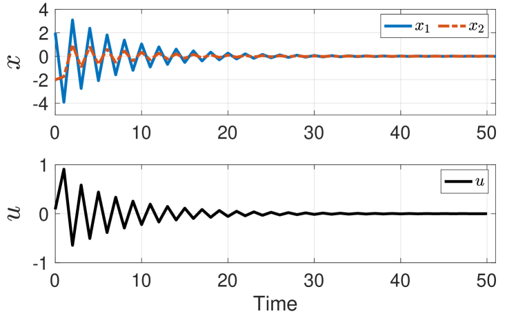
Figure 1: The optimal trajectory of a LQR system (50)-(51) using the weights $\boldsymbol{\omega}=[0.1,0.3,0.6]^{\prime}$.

5.1.1 Minimal Required Observations for IOC.

Based on the above LQR system, we here illustrate how the recovery matrix can be used to check whether incomplete trajectory data suffices for the minimal observation required for a successful weight estimation. Given the features $\boldsymbol{\phi^{*}}=[x_{1}^{2},x_{2}^{2},u^{2}]^{\prime}$, we set the observation starting time $t=0$, and incrementally increase the observation length $l$ from $1$ to horizon $T=50$. For each observation length $l$, we check the rank of the recovery matrix $\boldsymbol{H}(0,l)$ and solve the weights from the kernel of $\boldsymbol{H}(0,l)$ (the weights are normalized to have sum of one). The results are plotted in Fig. 2.

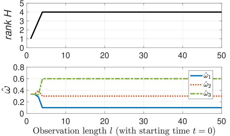
Figure 2: The rank of the recovery matrix and weight estimate when the observation starts at $t=0$ and the observation length $l$ increases from $1$ to $T$. The upper panel shows the rank of the recovery matrix $\boldsymbol{H}(0,l)$ versus $l$; and the bottom panel shows the corresponding weight estimate for each $l$. Note that the given features are $\boldsymbol{\phi^{*}}=[x_{1}^{2},x_{2}^{2},u^{2}]^{\prime}$ and the ground truth weights are $\boldsymbol{\omega}=[0.1,0.3,0.6]^{\prime}$. For $l<4$, since the dimension of the kernel of $\boldsymbol{H}(0,l)$ is at least 2 and thus $\boldsymbol{H}(0,l)[\hat{\boldsymbol{\omega}},\boldsymbol{\lambda}]^{\prime}=\boldsymbol{0}$ has multiple solutions of $[\hat{\boldsymbol{\omega}},\boldsymbol{\lambda}]^{\prime}$, we choose the solution $\hat{\boldsymbol{\omega}}$ from the kernel of $\boldsymbol{H}(0,l)$ randomly.

As shown in the upper panel in Fig. 2, including additional trajectory data points, i.e., increasing the observation length $l$ (from $1$), leads to an increase of the rank of the recovery matrix. When $l=4$ $\operatorname{rank}\boldsymbol{H}(0,l)$ reaches to $4$, which is the rank upper bound $n+r-1=4$, and then $\operatorname{rank}\boldsymbol{H}(0,l)=4$ for all $l\geq 4$. This illustrates the properties of the recovery matrix in Lemma 2 and Lemma 3. From the bottom panel in Fig. 2, we see that when $l<4$, for which $\operatorname{rank}\boldsymbol{H}(0,l)<4$, the weight estimate $\hat{\boldsymbol{\omega}}$ is not a successful estimate of $\boldsymbol{\omega}$. When $\operatorname{rank}\boldsymbol{H}(0,l)<4$, since the dimension of the kernel of $\boldsymbol{H}(0,l)$ is at least 2 and thus $\boldsymbol{H}(0,l)[\hat{\boldsymbol{\omega}},\boldsymbol{\lambda}]^{\prime}=\boldsymbol{0}$ has multiple solutions $[\hat{\boldsymbol{\omega}},\boldsymbol{\lambda}]^{\prime}$, we choose the solution $\hat{\boldsymbol{\omega}}$ from the kernel of $\boldsymbol{H}(0,l)$ randomly. After $l\geq 4$ when $\operatorname{rank}\boldsymbol{H}(0,l)=4$, the estimate converges to a successful estimate, thus indicating the effectiveness of using the rank condition in (45) to check whether an incomplete observation suffices for the minimal required observation.

(a) $t{=}5$, $\mathcal{F}=\{x_{1}^{2},x_{2}^{2},u^{2},u^{3}\}$

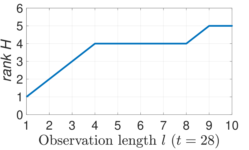
(b) $t{=}28$, $\mathcal{F}=\{x_{1}^{2},x_{2}^{2},u^{2},u^{3}\}$

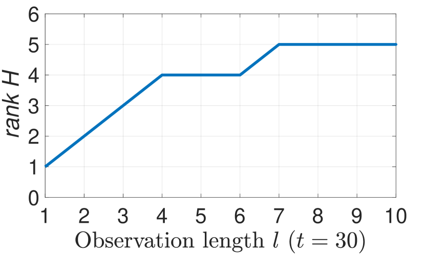
(c) $t{=}30$, $\mathcal{F}=\{x_{1}^{2},x_{2}^{2},u^{2},u^{3}\}$

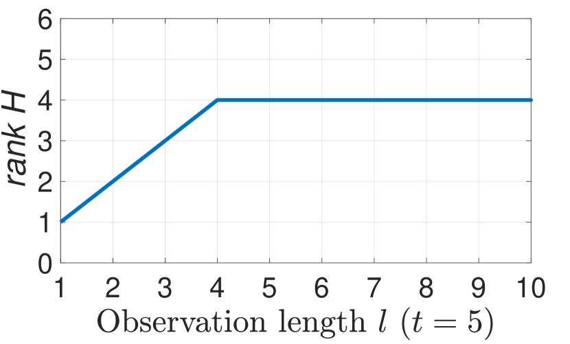
(d) $t{=}5$, $\mathcal{F}=\{x_{1}^{2},x_{2}^{2},u^{2},2u^{2}\}$

Figure 3: The rank of the recovery matrix versus the observation length $l$. For (a), (b), and (c), the observation starting time is at $t=5$, $t=28$, and $t=30$, respectively, and the given candidate feature set is $\mathcal{F}=\{x_{1}^{2},x_{2}^{2},u^{2},u^{3}\}$. For (d), the observation starting time is at $t=5$ and the given candidate feature set is $\mathcal{F}=\{x_{1}^{2},x_{2}^{2},u^{2},2u^{2}\}$. In (d), since $\mathcal{F}$ contains two dependent features: $u^{2}$ and $2u^{2}$, thus multiple combinations of these features can be found in $\mathcal{F}$ to characterize the optimal trajectory, that is, $\{x_{1}^{2},x_{2}^{2},u^{2}\}$ and $\{x_{1}^{2},x_{2}^{2},2u^{2}\}$, and the rank upper bound according to Lemma 3 is $\operatorname{rank}\boldsymbol{H}(t,l)<r+n-1=5$ and cannot reach $5$.

5.1.2 Recovery Matrix Rank for Additional Observations.

Based on the LQR system, we next show how additional observations affect the rank of the recovery matrix. Here, we vary the observation starting time $t$ and use different candidate feature sets $\mathcal{F}$, and for each case, we incrementally increase the observation length from $l=1$ while checking the rank of the recovery matrix until the rank reaches its maximum. The results are presented in Fig. 3. For the first three cases in Fig. 3(a)-3(c), we set the observation starting time at $t=5$, $t=28$, and $t=30$, respectively, and use a candidate feature set $\mathcal{F}=\{x_{1}^{2},x_{2}^{2},u^{2},u^{3}\}$; for the fourth case in Fig. 3(d), we set the observation starting time at $t=5$ and use a candidate feature set $\mathcal{F}=\{x_{1}^{2},x_{2}^{2},u^{2},2u^{2}\}$. Based on the results, we have the following observations and comments.

1) From Fig. 3(a), 3(b), and 3(c), we can see that additional observation (i.e., increasing observation length $l$) increases or maintains the rank of the recovery matrix, as stated in Lemma 2, and that continuously increasing the observation length will lead to the upper bound of the recovery matrix’s rank, as stated in Lemma 3.

2) Comparing Fig. 3(a) with Fig. 3(d), we see that although the number of candidate features for both cases are the same, i.e., $|\mathcal{F}|=r=4$, their corresponding maximum ranks are different: the case in Fig. 3(a) achieves $\max\operatorname{rank}\boldsymbol{H}=5=r+n-1$ (which is the rank condition (28) for a successful estimate), while in Fig. 3(d) the rank reaches $\max\operatorname{rank}\boldsymbol{H}=4<r+n-1$. This is because $\mathcal{F}=\{x_{1}^{2},x_{2}^{2},u^{2},2u^{2}\}$ used in Fig. 3(d) contains two dependent features, i.e., $u^{2}$ and $2u^{2}$, thus multiple combinations of features, e.g., $\{x_{1}^{2},x_{2}^{2},u^{2}\}$ and $\{x_{1}^{2},x_{2}^{2},2u^{2}\}$, can be found in $\mathcal{F}$ to characterize the optimal trajectory. Based on (34) in Lemma 3, $\operatorname{rank}\boldsymbol{H}(t,l)\leq 4$ for all $t$ and $l$ and the condition $\operatorname{rank}\boldsymbol{H}(t,l)=5=r+n-1$ for a successful recovery will never be fulfilled.

3) Comparing Fig. 3(b), Fig. 3(c) and Fig. 3(a), we note that in some cases additional observations will not increase the rank of the recovery matrix, e.g., when the observation length is $l=5,6,7,8$ in Fig. 3(b) and $l=5,6$ in Fig. 3(c). This can be explained using the following relations:

$$\operatorname{rank}\boldsymbol{H}(t,l+1)$$

$$=\operatorname{rank}\begin{bmatrix}\boldsymbol{H}_{1}(t,l)&\boldsymbol{H}_{2}(t,l)\\ \frac{\partial\boldsymbol{\phi}^{\prime}}{\partial\boldsymbol{u}^{*}_{t+l}}&\frac{\partial\boldsymbol{f}^{\prime}}{\partial\boldsymbol{u}^{*}_{t+l}}\end{bmatrix}\begin{bmatrix}I&\boldsymbol{0}\\ \frac{\partial\boldsymbol{\phi}^{\prime}}{\partial\boldsymbol{x}^{*}_{t+l+1}}&\frac{\partial\boldsymbol{f}^{\prime}}{\partial\boldsymbol{x}^{*}_{t+l+1}}\end{bmatrix}$$

$$=\operatorname{rank}\begin{bmatrix}\boldsymbol{H}_{1}(t,l)&\boldsymbol{H}_{2}(t,l)\\ \frac{\partial\boldsymbol{\phi}^{\prime}}{\partial\boldsymbol{u}^{*}_{t+l}}&\frac{\partial\boldsymbol{f}^{\prime}}{\partial\boldsymbol{u}^{*}_{t+l}}\end{bmatrix}$$

$$\geq\operatorname{rank}\begin{bmatrix}\boldsymbol{H}_{1}(t,l)&\boldsymbol{H}_{2}(t,l)\end{bmatrix}=\operatorname{rank}\boldsymbol{H}(t,l),$$

where the first two lines are directly from (30), and the last two lines are due to $\det(\frac{\partial\boldsymbol{f}^{\prime}}{\partial\boldsymbol{x}^{*}_{t+l+1}})=\det\begin{pmatrix}-1&0\\ 1&1\end{pmatrix}\neq 0$ and matrix rank properties. The above equation says that the new observation $\boldsymbol{\xi}_{t+l+1}=(\boldsymbol{x}^{*}_{t+l+1},\boldsymbol{u}^{*}_{t+l+1})$ is incorporated into the recovery matrix $\boldsymbol{H}(t,l)$ in the form of appending $m$ row vectors $[\frac{\partial\boldsymbol{\phi}^{\prime}}{\partial\boldsymbol{u}^{*}_{t+l}}\,\,\frac{\partial\boldsymbol{f}^{\prime}}{\partial\boldsymbol{u}^{*}_{t+l}}]\in\mathbb{R}^{m\times(r+n)}$ to the bottom of $\boldsymbol{H}(t,l)$. If the new observed data point $\boldsymbol{\xi}_{t+l+1}=(\boldsymbol{x}^{*}_{t+l+1},\boldsymbol{u}^{*}_{t+l+1})$ is non-informative, in other words, if the appended rows in $[\frac{\partial\boldsymbol{\phi}^{\prime}}{\partial\boldsymbol{u}^{*}_{t+l}}\,\,\frac{\partial\boldsymbol{f}^{\prime}}{\partial\boldsymbol{u}^{*}_{t+l}}]$ are dependent on the row vectors in $\boldsymbol{H}(t,l)$, then according to the matrix rank properties, one will have $\operatorname{rank}\boldsymbol{H}(t,l)=\operatorname{rank}\boldsymbol{H}(t,l+1)$, thus the new data $\boldsymbol{\xi}_{t+l+1}$ will not increase the rank of the recovery matrix. Otherwise, if the appended rows in $[\frac{\partial\boldsymbol{\phi}^{\prime}}{\partial\boldsymbol{u}^{*}_{t+l}}\,\,\frac{\partial\boldsymbol{f}^{\prime}}{\partial\boldsymbol{u}^{*}_{t+l}}]$ are independent of the row vectors in $\boldsymbol{H}(t,l)$, that is, the new observed data $\boldsymbol{\xi}_{t+l+1}=(\boldsymbol{x}^{*}_{t+l+1},\boldsymbol{u}^{*}_{t+l+1})$ is informative, then this new $\boldsymbol{\xi}_{t+l+1}$ will increase the rank of the recovery matrix, i.e., $\operatorname{rank}\boldsymbol{H}(t,l)<\operatorname{rank}\boldsymbol{H}(t,l+1)$.

5.1.3 Comparison with Prior Work.

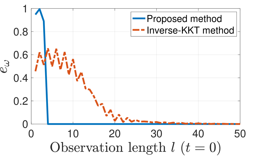
(a) Observation starting from $t=1$

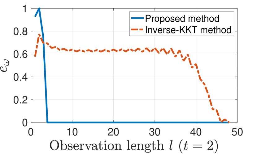
(b) Observation starting from $t=2$

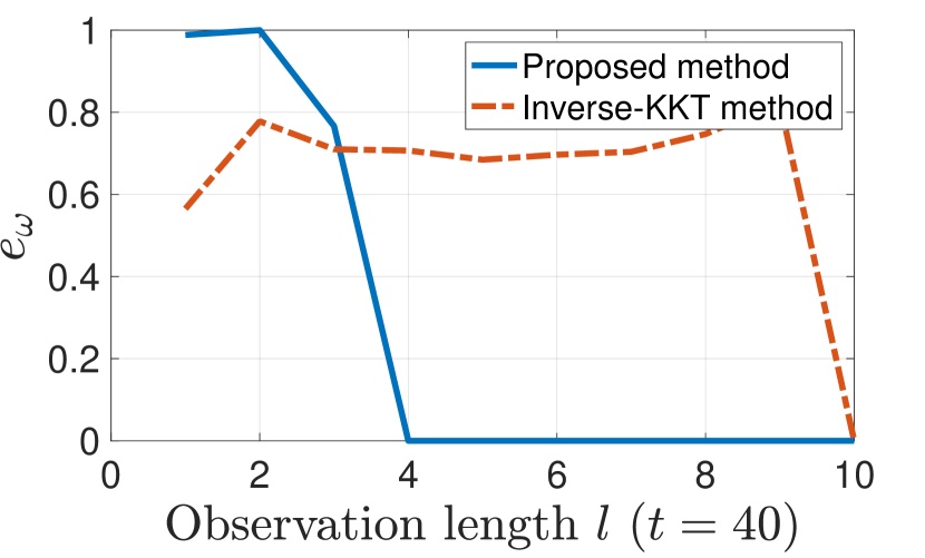
(c) Observation starting from $t=40$

Figure 4: Comparison between the inverse-KKT method (55) and proposed recovery matrix method (56) when given incomplete trajectory observation $\boldsymbol{\xi}_{t:t+l}$. Different observation starting time $t$ is used: $t=0$ in (a), $t=2$ in (b), and $t=40$ in (c). For each case, we increase the observation length $l$ from $1$ to the end of the horizon, i.e., $t+l=T$, and for each $l$, the estimation error $e_{\boldsymbol{\omega}}$ for both methods is evaluated, respectively. Note that the estimation error is defined in (49).

Here we demonstrate how the recovery matrix is able to solve IOC problems using incomplete observations. We will show this by comparing with a recent inverse-KKT method developed in (Englert et al., 2017). The idea of the inverse-KKT method is based on the optimality equations similar to (35) using full trajectory data $\boldsymbol{\xi}$. As suggested by (Englert et al., 2017), the weights are estimated by minimizing

$$\min_{\boldsymbol{\omega}}\lVert\boldsymbol{M}(\boldsymbol{\xi})\boldsymbol{\omega}\rVert^{2},$$ (53)

subject to $\sum_{i}{\omega}_{i}=1$. Although the inverse-KKT method (Englert et al., 2017) is developed based on full trajectory data $\boldsymbol{\xi}$, we here want to see its performance when only incomplete data $\boldsymbol{\xi}_{t:t+l}\subseteq\boldsymbol{\xi}$ is given.

As analyzed in Section 3.3, the coefficient matrix $\boldsymbol{M}(\boldsymbol{\xi})$ is a special case of the recovery matrix when $\boldsymbol{\xi}_{t:t+l}=\boldsymbol{\xi}_{0:T}$, that is,

$$\boldsymbol{M}(\boldsymbol{\xi})=\boldsymbol{H}_{1}(0,T).$$ (54)

Recall that this is because the LQR in (50)-(51) is a free-end optimal control system, as analyzed in Section 3.1, $\boldsymbol{\lambda}_{T+1}=\boldsymbol{0}$. Given incomplete observation data $\boldsymbol{\xi}_{t:t+l}\subseteq\boldsymbol{\xi}$, comparing the inverse-KKT method

$$\min_{\boldsymbol{\omega}}\lVert\boldsymbol{M}(\boldsymbol{\xi}_{t:t+l})\boldsymbol{\omega}\rVert^{2}\quad\text{s.t.}\quad\sum_{i}{\omega}_{i}=1,$$ (55)

with the proposed recovery matrix method

$$\min_{\boldsymbol{\omega},\boldsymbol{\lambda}}\lVert{\boldsymbol{H}}_{1}(t,l)\boldsymbol{\omega}+{\boldsymbol{H}}_{2}(t,l)\boldsymbol{\lambda}\rVert^{2}\quad\text{s.t.}\quad\sum_{i}{\omega}_{i}=1,$$ (56)

can show us how the unseen future data influences learning of the cost function.

For the LQR trajectory in Fig. 1, we use the feature set ${\mathcal{F}}=\{x_{1}^{2},x_{2}^{2},u^{2}\}$, set the observation starting time $t$ to be 0, 2, and 40, respectively, and for each observation starting time $t$, we increase the observation length $l$ from $1$ to the end of the trajectory, i.e., $t+l=T$. With each observation $\boldsymbol{\xi}_{t:t+l}$, we solve the weight estimate using the inverse-KKT method (55) and the proposed method (56) and evaluate the estimation error $e_{\boldsymbol{\omega}}$ in (49), respectively. Results are shown in Fig. 4, based on which we have the following comments.

1) The inverse-KKT method is sensitive to the starting time of the observation sequence. When the observation starts from $t=0$ (Fig. 4(a)), the inverse-KKT method achieves a successful estimate after observation length $l\geq 30$; when $t=2$ (Fig. 4(b)) and $t=40$ (Fig. 4(c)) only when $l$ reaches the end of trajectory, can the inverse-KKT method obtain the successful estimate.

2) As we have analyzed in Section 3.3, the success of the inverse-KKT method requires that the given data $\boldsymbol{\xi}_{t:t+l}$ itself minimizes the cost function, which is only guaranteed when the observation reaches the trajectory end, i.e., $t+l=T$. This explains the results in Fig. 4(b) and 4(c). Given incomplete $\boldsymbol{\xi}_{t:t+l}$ ($t+l<T$), although the inverse-KKT method still achieves a successful estimate in Fig. 4(a), such performance is not guaranteed and heavily relies on ‘informativeness’ of the given incomplete data relative to unseen future information. In Fig. 1, since the trajectory data at beginning phase is more ‘informative’ than the rest, the inverse-KKT method starting from $t=0$ uses less data to converge (Fig. 4(a)) than starting from $t=2$ (Fig. 4(b)).

3) In contrast, Fig. 4 shows the effectiveness of using the recovery matrix to deal with incomplete observations. The proposed method guarantees a successful estimate after a much smaller observation length (e.g., around $l=4$ for all three cases). This advantage is because the unseen future information is accounted for by $\boldsymbol{H}_{2}(t,l)$ in the recovery matrix and the related unknown future variable $\boldsymbol{\lambda}_{t+l+1}$ is jointly estimated in (56).

In sum, we make the following conclusions. First, existing KKT-based methods generally require a full trajectory, and cannot deal with incomplete trajectory data. Second, the proposed recovery matrix method addresses this by jointly accounting for unseen future information; and the recovery matrix presents a systematic way to check whether a trajectory segment is sufficient to recover the objective function and if so, to solve it only using the segment data. Third, existing KKT-based methods can be viewed as a special case of the proposed recovery matrix method when the segment data is the full trajectory.

5.1.4 IOC for Infinite-horizon LQR.

We demonstrate the ability of the proposed method to solve the IOC problem for an infinite-horizon control system. We still use the LQR system in (50)-(51) as an example, but here we set the time horizon $T=\infty$ (other conditions and parameters remain the same). The optimal trajectory in this case is a result of feedback control $\boldsymbol{u}=K\boldsymbol{x}$ with a constant control gain $K$ solved by the algebraic Riccati equation (Bertsekas, 1995). For the above infinite-horizon LQR (with $Q$ and $R$ in (52)), the control gain is solved as $K=[-0.1472\,\,-0.1918]$.

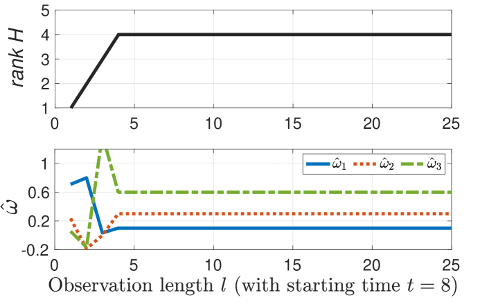
Figure 5: IOC results for infinite-horizon LQR system. The observation starting time is $t=8$ and the observation length $l$ increases from $l=1$ to $25$. The upper panel shows the rank of the recovery matrix versus increasing $l$, and the bottom panel is the corresponding weight estimate for each $l$.

In IOC, suppose that we observe an arbitrary segment from the infinite-horizon trajectory; here we use the segment data within the time interval $[t,t+l]=[8,33]$, namely, $\boldsymbol{\xi}_{8:33}$ with $t=8$ and $l=25$. We set the candidate feature set ${\mathcal{F}}=\{x_{1}^{2},x_{2}^{2},u^{2}\}$. The IOC results using Algorithm 1 are presented in Fig. 5. Here we fix the observation starting time $t=8$ while increasing $l$ from 1 to the time interval end $25$. The upper panel of Fig. 5 shows $\operatorname{rank}\boldsymbol{H}(8,l)$ versus increasing observation length $l$, and the bottom panel shows the weight estimate $\hat{\boldsymbol{\omega}}$ of each $l$ solved from the kernel of the recovery matrix $\boldsymbol{H}(8,l)$. As shown in the upper panel, with the observation length $l$ increasing, $\operatorname{rank}\boldsymbol{H}(8,l)$ quickly reaches the upper bound rank $r+n-1=4$ after $l\geq 4$, indicting the successful estimate of the weights as shown in the bottom panel. The results demonstrate the ability of the proposed method to solve IOC problems for infinite-horizon optimal control systems.

5.2 Evaluation on a Two-link Robot Arm

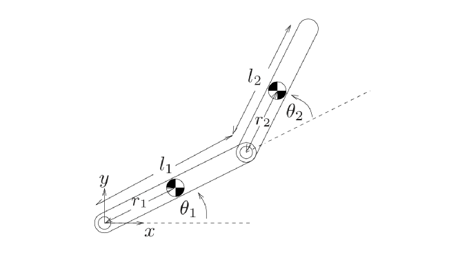
Figure 6: Two-link robot arm with coordinate definitions

To evaluate the proposed method on a non-linear plant, we use a two-link robot arm system, as shown in Fig. 6. The dynamics of the two-link arm (Spong and Vidyasagar, 2008, p. 209) moving in the vertical plane is

$$M(\boldsymbol{\theta})\ddot{\boldsymbol{\theta}}+C(\boldsymbol{\theta},\dot{\boldsymbol{\theta}})\dot{\boldsymbol{\theta}}+\boldsymbol{g}(\boldsymbol{\theta})=\boldsymbol{\tau},$$ (57)

where $\boldsymbol{\theta}=[\theta_{1},\theta_{2}]^{\prime}\in\mathbb{R}^{2}$ is the joint angle vector; $M(\boldsymbol{\theta})\in\mathbb{R}^{2\times 2}$ is the positive-definite inertia matrix; $C(\boldsymbol{\theta},\dot{\boldsymbol{\theta}})\in\mathbb{R}^{2\times 2}$ is the Coriolis matrix; $\boldsymbol{g}(\boldsymbol{\theta})\in\mathbb{R}^{2}$ is the gravity vector; and $\boldsymbol{\tau}=[\tau_{1},\tau_{2}]^{\prime}\in\mathbb{R}^{2}$ are the input torques applied to each joint. The parameters of the two-link robot arm in Fig. 6 are as follows. The mass of each link is $m_{1}=1\mathrm{kg}$, $m_{2}=1\mathrm{kg}$; the length of each link is $l_{1}=1\mathrm{m}$, $l_{2}=1\mathrm{m}$; the distance from the joint to the center of mass for each link is $r_{1}=0.5\mathrm{m}$, $r_{2}=0.5\mathrm{m}$; and the moment of inertia with respect to the center of mass for each link is $I_{1}=0.5\mathrm{kgm^{2}}$, $I_{2}=0.5\mathrm{kgm^{2}}$. From (57), we have

$$\ddot{\boldsymbol{\theta}}=M(\boldsymbol{\theta})^{-1}(-C(\boldsymbol{\theta},\dot{\boldsymbol{\theta}})\dot{\theta}-\boldsymbol{g}(\boldsymbol{\theta})+\boldsymbol{\tau}),$$ (58)

which can be further expressed in state-space representation

$$\dot{\boldsymbol{x}}=\boldsymbol{f}(\boldsymbol{x},\boldsymbol{u}),$$ (59)

with the system state and input defined as

$$\boldsymbol{x}=\begin{bmatrix}\theta_{1}&\theta_{2}&\dot{\theta_{1}}&\dot{\theta_{2}}\end{bmatrix}^{\prime},\quad\quad\boldsymbol{u}=\begin{bmatrix}\tau_{1}&\tau_{2}\end{bmatrix}^{\prime},$$ (60)

respectively. We consider the following finite-horizon fixed-end optimal control for the above robot arm system:

$$\underset{\boldsymbol{{x}}_{1:T}}{\text{min}} \sum_{k=0}^{T}\boldsymbol{\omega}\boldsymbol{\phi}^{*}(\boldsymbol{x}_{k},\boldsymbol{u}_{k}),$$ (61)

s.t. $$\boldsymbol{x}_{k+1}=\boldsymbol{x}_{k}+\Delta\boldsymbol{f}(\boldsymbol{x}_{k},\boldsymbol{u}_{k}),$$

$$\boldsymbol{x}_{0}=\boldsymbol{x}_{\text{start}},$$

$$\boldsymbol{x}_{T+1}=\boldsymbol{x}_{\text{goal}},$$

where $\Delta=0.01\mathrm{s}$ is the discretization interval. In (61), we specify the initial state $\boldsymbol{x}_{\text{start}}=[0,0,0,0]^{\prime}$, goal state $\boldsymbol{x}_{\text{goal}}=[\frac{\pi}{2},-\frac{\pi}{2},0,0]^{\prime}$, the time horizon $T=100$, and the feature vector and the corresponding weights

$$\boldsymbol{\phi}^{*}=\begin{bmatrix}\tau_{1}^{2}&\tau_{2}^{2}&\tau_{1}\tau_{2}\end{bmatrix}^{\prime}\quad\boldsymbol{\omega}=\begin{bmatrix}0.6&0.3&0.1\end{bmatrix}^{\prime},$$ (62)

respectively. We solve the above optimal control system (61) using the CasADi software (Andersson et al., 2019) and plot the resulting trajectory in Fig. 7.

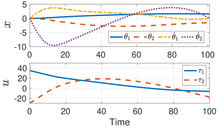
Figure 7: The optimal trajectory of the two-link robot arm optimal control system (61) with the cost function (62).

5.2.1 Minimal Required Observations for IOC.

Based on the above robot arm system, we first show the use of the recovery matrix to check whether an incomplete trajectory observation suffices for the minimal observation required for successful IOC. As an example, in Fig. 7, we set the observation starting time at $t=50$. While increasing the observation length $l$ from $1$, we check the rank of $\boldsymbol{H}(50,l)$, solve the weight estimate $\hat{\boldsymbol{\omega}}$ from the kernel of $\boldsymbol{H}(50,l)$, and evaluate the estimation error $e_{\boldsymbol{\omega}}$ in (49) for $\hat{\boldsymbol{\omega}}$. This process is repeated for three different candidate feature sets: $\mathcal{F}=\{\tau_{1}^{2},\tau_{2}^{2},\tau_{1}\tau_{2}\},\mathcal{F}=\{\tau_{1}^{2},\tau_{2}^{2},\tau_{1}\tau_{2},\tau_{1}^{3},\tau_{2}^{3},\tau_{1}^{2}\tau_{2}\},$ and $\mathcal{F}=\{\tau_{1}^{2},\tau_{2}^{2},\tau_{1}\tau_{2},\tau_{1}^{3},\tau_{2}^{3},\tau_{1}\tau_{2}^{2},\tau_{1}^{4},\tau_{2}^{4},\tau_{1}^{3}\tau_{2},\tau_{1}^{2}\tau_{2}^{2}\}$, respectively. The results are shown in Fig. 8.

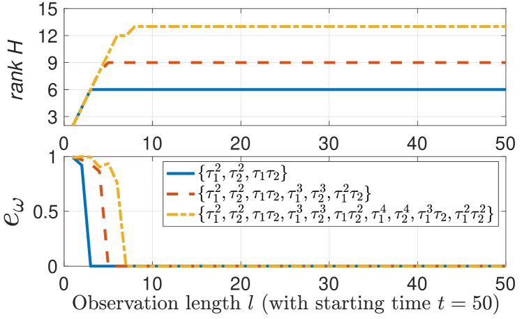
Figure 8: The rank of the recovery matrix and corresponding estimation error $e_{\boldsymbol{\omega}}$ under different observation length $l$ and different candidate feature sets. The upper panel shows the rank of the recovery matrix versus $l$, and the bottom panel shows the estimation error $e_{\boldsymbol{\omega}}$ for each $l$. Three feature sets, $\mathcal{F}=\{\tau_{1}^{2},\tau_{2}^{2},\tau_{1}\tau_{2}\},\mathcal{F}=\{\tau_{1}^{2},\tau_{2}^{2},\tau_{1}\tau_{2},\tau_{1}^{3},\tau_{2}^{3},\tau_{1}^{2}\tau_{2}\},$ and $\mathcal{F}=\{\tau_{1}^{2},\tau_{2}^{2},\tau_{1}\tau_{2},\tau_{1}^{3},\tau_{2}^{3},\tau_{1}\tau_{2}^{2},\tau_{1}^{4},\tau_{2}^{4},\tau_{1}^{3}\tau_{2},\tau_{1}^{2}\tau_{2}^{2}\}$, are used, respectively, and the corresponding results are plotted in different lines. Note that when $\operatorname{rank}\boldsymbol{H}(50,l)<|\mathcal{F}|+n-1$, since the dimension of the kernel of $\boldsymbol{H}(50,l)$ is at least 2, we thus choose $\hat{\boldsymbol{\omega}}$ from the kernel of $\boldsymbol{H}(50,l)$ randomly.

Results in the upper panel of Fig. 8 show that additional observations increase the rank of the recovery matrix. Once the additional observations lead to the upper-bound rank of the recovery matrix, i.e., $|\mathcal{F}|+n-1$, the corresponding length is the minimal observation length $l_{\min}(t)$ required for a successful weight estimate, as shown in the corresponding bottom panel in Fig. 8. Moreover, including additional irrelevant features in $\mathcal{F}$ will lead to the increased minimal required observation length $l_{\min}(t)$, as implied by (46). This will be discussed later in Section 5.2.3.

5.2.2 Observation Noise.

We test the proposed incremental IOC approach (Algorithm 1) under different data noise levels. We add to the trajectory in Fig. 7 Gaussian noise of different levels that are characterized by different standard deviations from $\sigma=10^{-5}$ to $\sigma=10^{-1}$. In Algorithm 1, we use $\mathcal{F}=\{{\tau}^{2}_{1},{\tau}^{2}_{2},\tau_{1}\tau_{2}\}$ and set $\gamma=45$ (the choice of $\gamma$ will be discussed later in Section 5.2.4).

We set the observation starting time $t$ at all time instants except for those near the trajectory end which can not provide sufficient subsequent observation length. As an example, we present the experimental results for the case of noise level $\sigma=10^{-2}$ in Fig 9. Here, the upper panel shows the minimal required observation length $l_{\min}(t)$ automatically found for each observation starting time $t$, and the bottom shows the corresponding weight estimate using the minimal required observation data $\boldsymbol{\xi}_{t:t+l_{\min}(t)}$.

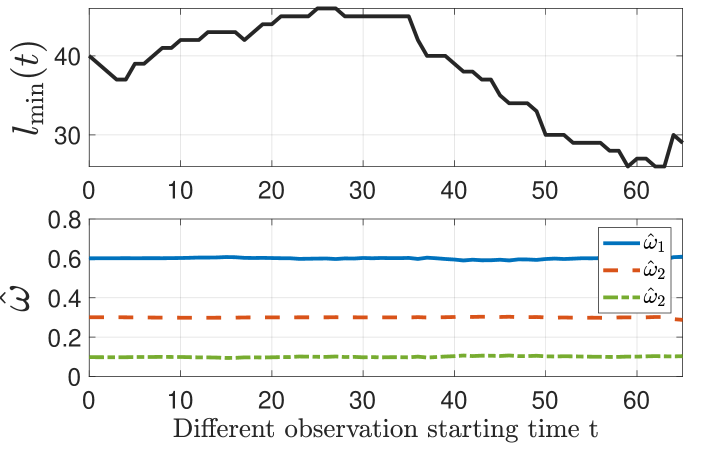
Figure 9: IOC by automatically finding the minimal required observation under noise level $\sigma=10^{-2}.$ The x-axis is the different observation starting time $t$. The upper panel shows the automatically-found minimal required observation length $l_{\min}(t)$ at different $t$, and the bottom panel shows the corresponding estimate $\boldsymbol{\hat{\omega}}$ via (47). Note that ground truth $\boldsymbol{\omega}=[0.6,0.3,0.1]^{\prime}$.

From Fig. 9, we see that the automatically-found minimal required observation length $l_{\min}(t)$ varies depending on the observation starting time $t$. This can be interpreted by noting that the trajectory data in Fig. 7 in different intervals has different informativeness to reflect the cost function. For example, according to Fig. 9, we can postulate that the beginning and final portions of the trajectory data are more ‘data-informative’ than other portions, thus needing smaller $l_{\min}(t)$ to achieve the successful estimate. This can be understood if we consider that the beginning and final portions of the trajectory in Fig. 7 has richer patterns such as curvatures than the middle which are more smooth. Using the recovery matrix, the data informativeness about the cost function is quantitatively indicated by the recovery matrix’s rank. Even under observation noise, the proposed method can adaptively find the sufficient observation length size such that the data is informative enough to guarantee a successful estimate of the weights, as shown by both upper and bottom panels in Fig. 9.

Table 1: Results of incremental IOC (Algorithm 1, $\gamma=45$) under different noise levels.

Noise level $\sigma$	Averaged $l_{\min}/T$ (%) †	Averaged $e_{\boldsymbol{\omega}}$†
$\sigma=10^{-5}$	$8\%$	$4.3\times 10^{-4}$
$\sigma=10^{-4}$	$8.1\%$	$4.0\times 10^{-3}$
$\sigma=10^{-3}$	$12.61\%$	$8.1\times 10^{-3}$
$\sigma=10^{-2}$	$33.8\%$	$8.5\times 10^{-3}$
$\sigma=10^{-1}$	$70.0$%	$7.1\times 10^{-3}$

• The average is calculated based on all successful estimations over all observation cases (varying observation starting time).

We summarize all results under different noise levels in Table 1. Here the minimal required observation length is presented in percentage with respect to the total horizon $T$. According to Table 1, under a fixed rank index threshold (here $\gamma=45$), we can see that high noise levels, on average, will lead to larger minimal required observation length, but the estimation error is not influenced too much. This is because the increased observation length can compensate for the uncertainty induced by data noise and finally produces a ‘neutralized’ estimate. Hence, the results prove the robustness of the proposed incremental IOC algorithm against the small observation noise. We will later show how to further improve the accuracy by adjusting $\gamma$.

5.2.3 Presence of Irrelevant Features.

We here assume that exact knowledge of relevant features is not available, and we evaluate the performance of Algorithm 1 given a feature set including irrelevant features. We add all observation data with Gaussian noise of $\sigma=10^{-3}$. In Algorithm 1, we set $\gamma=45$ and construct a feature set $\mathcal{F}$ based on the following candidate features

$$\{\tau_{1}^{2},\,\tau_{2}^{2},\,\tau_{1}\tau_{2},\,\,\,\tau_{1}^{3},\,\tau_{2}^{3},\,\tau_{1}\tau_{2}^{2},\,\tau_{1}^{2}\tau_{2},\,\\ \tau_{1}^{4},\tau_{2}^{4},\,\,\tau_{1}^{3}\tau_{2},\,\,\tau_{1}\tau_{2}^{3},\,\,\tau_{1}^{2}\tau_{2}^{2}\}.$$ (63)

Algorithm 1 is applied the same way as in the previous experiment: by starting the observation at all time instants except for those near the trajectory end. We provide different candidate feature sets in the first column in Table 2, and for each case we compute the average of the minimal required observation length and the average of estimation error in (49). The results are summarized in second and third columns in Table 2.

Table 2: Results of incremental IOC (Algorithm 1, $\gamma=45$) with different given feature sets.

Candidate feature set $\mathcal{F}$	Averaged $l_{\min}/T$1	Averaged $e_{\boldsymbol{\omega}}$1
$\{\tau_{1}^{2},\,\tau_{2}^{2},\,\tau_{1}\tau_{2}\}$	$12.18\%$	$4.2\times 10^{-3}$
$\begin{aligned} \{\tau_{1}^{2},\,\tau_{2}^{2},\,\tau_{1}\tau_{2},\,\tau_{1}^{3},\tau_{2}^{3}\}\end{aligned}$	$14.7\%$	$9.7\times 10^{-3}$
$\begin{aligned} \{&\tau_{1}^{2},\,\tau_{2}^{2},\,\tau_{1}\tau_{2},\,\tau_{1}^{3},\tau_{2}^{3},\\[-3.0pt] &\tau_{1}\tau_{2}^{2},\,\tau_{1}^{2}\tau_{2}\}\end{aligned}$	$25.69\%$	$8.7\times 10^{-3}$
$\begin{aligned} \{&\tau_{1}^{2},\,\tau_{2}^{2},\,\tau_{1}\tau_{2},\,\tau_{1}^{3},\tau_{2}^{3},\\[-3.0pt] &\tau_{1}\tau_{2}^{2},\,\tau_{1}^{2}\tau_{2},\tau_{1}^{4},\tau_{2}^{4}\}\end{aligned}$	$35.97\%$	$8.6\times 10^{-3}$
$\begin{aligned} \{&\tau_{1}^{2},\,\tau_{2}^{2},\,\tau_{1}\tau_{2},\,\tau_{1}^{3},\tau_{2}^{3},\\[-3.0pt] &\tau_{1}\tau_{2}^{2},\,\tau_{1}^{2}\tau_{2},\tau_{1}^{4},\tau_{2}^{4},\\[-3.0pt] &\tau_{1}^{3}\tau_{2},\,\tau_{1}\tau_{2}^{3},\,\tau_{1}^{2}\tau_{2}^{2}\}\end{aligned}$	$45.53\%$	$9.1\times 10^{-3}$

• The average is calculated based on all successful estimations over all observation cases (varying observation starting time).

Table 2 indicates that on average, the minimal required observation length increases as additional irrelevant features are included to the feature set $\mathcal{F}$. This can be understood if we consider (45) and the rank non-decreasing property in Lemma 2: when a certain number of irrelevant features are added, the rank required for successful estimate will increase by the same amount, thus needing additional trajectory data points. Due to increased observation length, the estimation accuracy is not much influenced by the additional irrelevant features. Thus we conclude that the proposed incremental IOC algorithm applies to the presence of irrelevant features.

5.2.4 Parameter Setting.

We now discuss how to choose the rank threshold $\gamma$ in Algorithm 1. Since in Algorithm 1 the rank index (41) for the recovery matrix is used to find the minimal required observation length, we first investigate how the rank index $\kappa(t,l)$ changes as the observation length $l$ increases. We use the trajectory data in Fig. 7 with added Gaussian noise of $\sigma=10^{-3}$, $\sigma=2\times 10^{-3}$, and $\sigma=10^{-2}$, respectively. The candidate features set here is $\mathcal{F}=\{\tau_{1}^{2},\tau_{2}^{2},\tau_{1}\tau_{2}\}$. We fix the observation start time $t=0$ and increase the observation length $l$ from $1$ to $T$. The rank index $\kappa(t=0,l)$ for different $l$ is shown in Fig. 10.

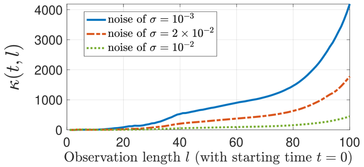
Figure 10: The rank index $\kappa(0,l)$ in (41) versus different observation length $l$ under different noise levels.

From Fig. 10, we can see that although $\kappa(t,l)$ has different scales at different noise levels, it in general increases as the observation length $l$ increases. This can be understood if we compare the above results to $\kappa(t,l)$ in noise-free cases: when there is no data noise, according to Lemma 2 and 3, as $l$ increases, $\kappa(t,l)$ will first remain zero when $l<l_{\min}$, then increase to infinity after $l\geq l_{\min}$. In noisy settings, $\kappa(t,l)$ however will increase to a large finite value. From the plot, we can postulate that in practice choosing a larger threshold $\gamma$ will lead to a larger minimal required observation length $l_{\min}$, thus more data points will be included into the recovery matrix to compute the estimate of the weights, which may finally improve the estimation accuracy (similar to results in Table 1). In what follows, we will verify this postulation by showing how $\gamma$ affects the performance of Algorithm 1.

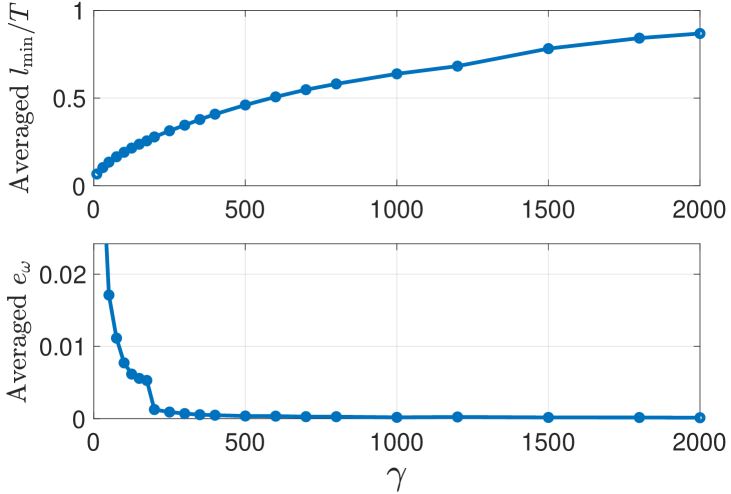
Figure 11: Averaged $l_{\min}$ (upper panel) and averaged estimation error $e_{\boldsymbol{\omega}}$ (bottom panel) for different choices of $\gamma$.

We add Gaussian noise $\sigma=10^{-3}$ to the trajectory data in Fig. 7, and apply Algorithm 1 by starting the observation at all possible time steps, as performed in previous experiments. We vary $\gamma$ to show its influence on the average of the minimal required observation length $l_{\min}$ and the average of the estimation error $e_{\boldsymbol{\omega}}$. The results are shown in Fig. 11, from which we can observe that first, a larger $\gamma$ will lead to larger minimal required observation length; and second, due to the increased minimal required observation, the corresponding estimation accuracy is improved because data noise or other error sources can be compensated by additional observation data. These facts thus prove our previous postulation based on Fig. 10. Moreover, Fig. 11 also shows as $\gamma$ exceeds a certain value, e.g., 200, continuously increasing $\gamma$ will not improve the recovery accuracy significantly. This suggests that the choice of $\gamma$ is not sensitive to the performance if $\gamma$ is large. Therefore, in practice it is possible to find a proper $\gamma$ without much manual effort such that both the estimation accuracy and computational cost are balanced.

6 Conclusions

This article considers the problem of learning an objective function from an observation of an incomplete trajectory. To achieve this goal, we develop the recovery matrix, which establishes a relationship between trajectory segment data and the unknown weights of given candidate features. The rank of the recovery matrix indicates whether an incomplete trajectory observation is sufficient for obtaining a successful estimate of the weights. By investigating the properties of the recovery matrix, we further demonstrate that additional observations may increase the rank of the recovery matrix, thus contributing to enabling the successful estimation, and that the IOC can be processed incrementally. Based on the recovery matrix, a method for using incomplete trajectory observations to estimate the weights of specified features is established, and an incremental IOC algorithm is developed by automatically finding the minimal required observation.

This research is partly supported by the ERC Consolidator Grant Safe data-driven control for human-centric systems under grant agreement 864686 at Chair of Information-oriented Control, Technical University of Munich.

Appendix A Proof of Lemma 1

Consider the recovery matrix $\boldsymbol{H}(t,l)$ for the trajectory segment $\boldsymbol{\xi}_{{t:t+l}}=(\boldsymbol{x}^{*}_{{t:t+l}}\boldsymbol{u}^{*}_{{t:t+l}})$, with $t$ being the observation starting time and $l$ being the observation length. When a subsequent point $\boldsymbol{\xi}_{t+l+1}=(\boldsymbol{x}^{*}_{{t:t+l+1}},\boldsymbol{u}^{*}_{{t:t+l+1}})$ is observed, from Definition 1, the updated recovery matrix is $\boldsymbol{H}(t,l+1)=[\boldsymbol{H}_{1}(t,l+1),\boldsymbol{H}_{2}(t,l+1)]$, where

$$\boldsymbol{H}_{1}(t,l+1)=\boldsymbol{F}_{u}(t,l+1)\boldsymbol{F}^{-1}_{x}(t,l+1)\boldsymbol{\Phi}_{x}(t,l+1)\\ +\boldsymbol{\Phi}_{u}(t,l+1),$$ (64)

and

$$\boldsymbol{H}_{2}(t,l+1)=\boldsymbol{F}_{u}(t,l+1)\boldsymbol{F}_{x}^{-1}(t,l+1)\boldsymbol{V}(t,l+1).$$ (65)

Here $\boldsymbol{F}_{x}(t,l+1)$, $\boldsymbol{F}_{u}(t,l+1)$, $\boldsymbol{\Phi}_{x}(t,l+1)$, $\boldsymbol{\Phi}_{u}(t,l+1)$, and $\boldsymbol{V}(t,l+1)$, defined in (9)-(13), are updated as follow:

$$\boldsymbol{\Phi}_{{u}}(t,l+1) =\begin{bmatrix}\boldsymbol{\Phi}_{u}(t,l)\\ \frac{\partial\boldsymbol{\phi}^{\prime}}{\partial\boldsymbol{u}^{*}_{t+l}}\end{bmatrix},$$ (66a)

$$\boldsymbol{\Phi}_{x}(t,l+1) =\begin{bmatrix}\boldsymbol{\Phi}_{x}(t,l)\\ \frac{\partial\boldsymbol{\phi}^{\prime}}{\partial\boldsymbol{x}^{*}_{{t:t+l+1}}}\end{bmatrix},$$ (66b)

$$\boldsymbol{F}_{u}(t,l+1) =\begin{bmatrix}\boldsymbol{F}_{u}(t,l)&\boldsymbol{0}\\ \boldsymbol{0}&\frac{\partial\boldsymbol{f}^{\prime}}{\partial\boldsymbol{u}^{*}_{t+l}}\end{bmatrix},$$ (66c)

$$\boldsymbol{F}_{x}^{-1}(t,l+1) =\begin{bmatrix}\boldsymbol{F}_{x}(t,l)&-\boldsymbol{V}(t,l)\\ \boldsymbol{0}&\boldsymbol{I}\end{bmatrix}^{-1}$$

$$=\begin{bmatrix}\boldsymbol{F}_{x}^{-1}(t,l)&\boldsymbol{F}_{x}^{-1}(t,l)\boldsymbol{V}(t,l)\\ \boldsymbol{0}&\boldsymbol{I}\end{bmatrix},$$ (66d)

respectively. Here (66d) is based on the fact

$$\begin{bmatrix}A&B\\ C&D\end{bmatrix}^{-1}=\begin{bmatrix}A^{-1}+A^{-1}BK^{-1}CA^{-1}&-A^{-1}BK^{-1}\\ -K^{-1}CA^{-1}&K^{-1}\end{bmatrix}$$

with $K=D-CA^{-1}B$ being the Schur complement of the above block matrix with respect to $A$. Combining (66a)-(66d), we have

$$\begin{split}\boldsymbol{H}_{1}(t,l+1)&=\boldsymbol{F}_{u}(t,l+1)\boldsymbol{F}_{x}^{-1}(t,l+1)\boldsymbol{\Phi}_{x}(t,l+1)\\ &\qquad+\boldsymbol{\Phi}_{u}(t,l+1)\end{split}$$

$$\begin{split}&=\begin{bmatrix}\boldsymbol{F}_{u}(t,l)\boldsymbol{F}_{x}^{-1}(t,l)\boldsymbol{\Phi}_{x}(t,l)+\boldsymbol{\Phi}_{u}(t,l)\\ \frac{\partial\boldsymbol{f}^{\prime}}{\partial\boldsymbol{u}^{*}_{t+l}}\frac{\partial\boldsymbol{\phi}^{\prime}}{\partial\boldsymbol{x}^{*}_{{t+l+1}}}+\frac{\partial\boldsymbol{\phi}^{\prime}}{\partial\boldsymbol{u}^{*}_{t+l}}\end{bmatrix}\\ &+\begin{bmatrix}\boldsymbol{F}_{u}(t,l)\boldsymbol{F}_{x}^{-1}(t,l)\boldsymbol{V}(t,l)\frac{\partial\boldsymbol{\phi}^{\prime}}{\partial\boldsymbol{x}^{*}_{{t+l+1}}}\\ \boldsymbol{0}\end{bmatrix}.\end{split}$$ (67)

Combining with (7)-(8), the above (A) becomes

$$\boldsymbol{H}_{1}(t,l+1) =\begin{bmatrix}\boldsymbol{H}_{1}(t,l)+\boldsymbol{H}_{2}(t,l)\frac{\partial\boldsymbol{\phi}^{\prime}}{\partial\boldsymbol{x}^{*}_{{t+l+1}}}\\ \frac{\partial\boldsymbol{f}^{\prime}}{\partial\boldsymbol{u}^{*}_{t+l}}\frac{\partial\boldsymbol{\phi}^{\prime}}{\partial\boldsymbol{x}^{*}_{{t+l+1}}}+\frac{\partial\boldsymbol{\phi}^{\prime}}{\partial\boldsymbol{u}^{*}_{t+l}}\end{bmatrix}.$$ (68)

Considering (66a)-(66d), we have

$$\boldsymbol{H}_{2}(t,l+1) =\boldsymbol{F}_{u}(t,l+1)\boldsymbol{F}_{x}^{-1}(t,l+1)\boldsymbol{V}(t,l+1)$$

$$=\begin{bmatrix}\boldsymbol{F}_{u}(t,l)\boldsymbol{F}_{x}^{-1}(t,l)\boldsymbol{V}(t,l)\frac{\partial\boldsymbol{f}^{\prime}}{\partial\boldsymbol{x}^{*}_{{t+l+1}}}\\ \frac{\partial\boldsymbol{f}^{\prime}}{\partial\boldsymbol{u}^{*}_{t+l}}\frac{\partial\boldsymbol{f}^{\prime}}{\partial\boldsymbol{x}^{*}_{{t+l+1}}}\end{bmatrix}$$

$$=\begin{bmatrix}\boldsymbol{H}_{2}(t,l)\frac{\partial\boldsymbol{f}^{\prime}}{\partial\boldsymbol{x}^{*}_{{t+l+1}}}\\ \frac{\partial\boldsymbol{f}^{\prime}}{\partial\boldsymbol{u}^{*}_{t+l}}\frac{\partial\boldsymbol{f}^{\prime}}{\partial\boldsymbol{x}^{*}_{{t+l+1}}}\end{bmatrix}.$$ (69)

Finally joining (68) and (A) and writing them in the matrix form lead to (30).

When $l=1$, that is, $\boldsymbol{\xi}_{t:t+1}=(\boldsymbol{x}^{*}_{t:t+1},\boldsymbol{u}^{*}_{t:t+1})$ is available, we have $\boldsymbol{F}_{x}(t,1)=I$, $\boldsymbol{F}_{u}(t,1)=\frac{\partial\boldsymbol{f}^{\prime}}{\partial\boldsymbol{u}^{*}_{t}}$, $\boldsymbol{\Phi}_{x}(t,1)=\frac{\partial\boldsymbol{\phi}^{\prime}}{\partial\boldsymbol{x}^{*}_{t+1}}$, $\boldsymbol{\Phi}_{u}(t,1)=\frac{\partial\boldsymbol{\phi}^{\prime}}{\partial\boldsymbol{u}^{*}_{t}}$, and $\boldsymbol{V}(t,1)=\frac{\partial\boldsymbol{f}^{\prime}}{\partial\boldsymbol{x}^{*}_{t+1}}$. According to the definition of recovery matrix in (6)-(8), we thus obtain (1). This completes the proof.  

Appendix B Proof of Lemma 2

From Lemma 1, we have

$$\operatorname{rank}\boldsymbol{H}(t,l+1)$$

$$=\operatorname{rank}\begin{bmatrix}\boldsymbol{H}_{1}(t,l)&\boldsymbol{H}_{2}(t,l)\\ \frac{\partial\boldsymbol{\phi}^{\prime}}{\partial\boldsymbol{u}^{*}_{t+l}}&\frac{\partial\boldsymbol{f}^{\prime}}{\partial\boldsymbol{u}^{*}_{t+l}}\end{bmatrix}\begin{bmatrix}I&\boldsymbol{0}\\ \frac{\partial\boldsymbol{\phi}^{\prime}}{\partial\boldsymbol{x}^{*}_{{t+l+1}}}&\frac{\partial\boldsymbol{f}^{\prime}}{\partial\boldsymbol{x}^{*}_{{t+l+1}}}\end{bmatrix}.$$ (70)

If $\det(\frac{\partial\boldsymbol{f}}{\partial\boldsymbol{x}^{*}_{{t+l+1}}})\neq 0$, the last block matrix in (70) is non-singular. Consequently

$$\operatorname{rank}\boldsymbol{H}(t,l+1) =\operatorname{rank}\begin{bmatrix}\boldsymbol{H}_{1}(t,l)&\boldsymbol{H}_{2}(t,l)\\ \frac{\partial\boldsymbol{\phi}^{\prime}}{\partial\boldsymbol{u}^{*}_{t+l}}&\frac{\partial\boldsymbol{f}^{\prime}}{\partial\boldsymbol{u}^{*}_{t+l}}\end{bmatrix}$$

$$\geq\operatorname{rank}\begin{bmatrix}\boldsymbol{H}_{1}(t,l)&\boldsymbol{H}_{2}(t,l)\end{bmatrix}$$

$$=\operatorname{rank}\boldsymbol{H}(t,l).$$ (71)

Note that both (70) and the inequality (B) are independent of the choice of $\boldsymbol{\phi}$. This completes the proof.  

Appendix C Proof of Lemma 3

We first prove (33). Without losing generality, we consider the feature set in (14). For any trajectory segment $\boldsymbol{\xi}_{t:{t+l}}\subseteq\boldsymbol{\xi}$, from (27), we have known that there exists a costate $\boldsymbol{\lambda}_{{t+l+1}}^{*}$ such that

$$\boldsymbol{H}(t,l)\begin{bmatrix}\bar{\boldsymbol{\omega}}\\ \boldsymbol{\lambda}_{{t+l+1}}^{*}\end{bmatrix}=\boldsymbol{0}$$ (72)

holds, where $\bar{\boldsymbol{\omega}}\neq\boldsymbol{0}$ is defined in (16). Thus, the nullity of $\boldsymbol{H}(t,l)$ is at least one, which means

$$\operatorname{rank}\boldsymbol{H}(t,l)\leq r+n-1.$$

We then prove (34). When another relevant feature subset $\mathcal{\widetilde{F}}$ exists in $\mathcal{F}$ with associated weight vector $\boldsymbol{\widetilde{\omega}}$, we can similarly construct a weight vector $\breve{\boldsymbol{\omega}}$ corresponding to ${\rm col\;}\mathcal{F}$ as in (16); that is, the weights in $\breve{\boldsymbol{\omega}}$ that correspond to $\mathcal{\widetilde{F}}$ are from $\boldsymbol{\widetilde{\omega}}$ and otherwise zeros. Then following the similar derivations as from (17) to (27), we can obtain that there exists $\breve{\boldsymbol{\lambda}}_{{t+l+1}}\in\mathbb{R}^{n}$ such that

$$\boldsymbol{H}(t,l)\begin{bmatrix}\breve{\boldsymbol{\omega}}\\ \breve{\boldsymbol{\lambda}}_{{t+l+1}}\end{bmatrix}=\boldsymbol{0}.$$ (73)

Since $\mathcal{\widetilde{F}}\neq\mathcal{F^{*}}$ or $\boldsymbol{\widetilde{\omega}}\neq c_{1}\boldsymbol{\omega}$ implies $\breve{\boldsymbol{\omega}}\neq c_{2}\bar{\boldsymbol{\omega}}$ ($c_{1}$ and $c_{2}$ are some nonzero scalars), based on (72) and (73), it follows that the nullity of $\boldsymbol{H}(t,l)$ is at least two, i.e.,

$$\operatorname{rank}\boldsymbol{H}(t,l)\leq r+n-2.$$

This completes the proof.

References

- Abbeel et al. (2010) Abbeel P, Coates A and Ng AY (2010) Autonomous helicopter aerobatics through apprenticeship learning. The International Journal of Robotics Research 29(13): 1608–1639.
- Abbeel and Ng (2004) Abbeel P and Ng AY (2004) Apprenticeship learning via inverse reinforcement learning. In: International Conference on Machine learning.
- Aghasadeghi and Bretl (2014) Aghasadeghi N and Bretl T (2014) Inverse optimal control for differentially flat systems with application to locomotion modeling. In: IEEE International Conference on Robotics and Automation. pp. 6018–6025.
- Andersson et al. (2019) Andersson JAE, Gillis J, Horn G, Rawlings JB and Diehl M (2019) CasADi – A software framework for nonlinear optimization and optimal control. Mathematical Programming Computation 11(1): 1–36.
- Bajcsy et al. (2018) Bajcsy A, Losey DP, O’Malley MK and Dragan AD (2018) Learning from physical human corrections, one feature at a time. In: ACM/IEEE International Conference on Human-Robot Interaction. pp. 141–149.
- Bajcsy et al. (2017) Bajcsy A, Losey DP, O’Malley MK and Dragan AD (2017) Learning robot objectives from physical human interaction. Proceedings of Machine Learning Research 78: 217–226.
- Berret et al. (2011) Berret B, Chiovetto E, Nori F and Pozzo T (2011) Evidence for composite cost functions in arm movement planning: an inverse optimal control approach. PLoS computational biology 7(10).
- Bertsekas (1995) Bertsekas DP (1995) Dynamic programming and optimal control, volume 1. Athena scientific Belmont, MA.
- Boyd and Vandenberghe (2004) Boyd S and Vandenberghe L (2004) Convex optimization. Cambridge university press.
- Clever et al. (2016) Clever D, Schemschat RM, Felis ML and Mombaur K (2016) Inverse optimal control based identification of optimality criteria in whole-body human walking on level ground. In: IEEE International Conference on Biomedical Robotics and Biomechatronics. pp. 1192–1199.
- Englert et al. (2017) Englert P, Vien NA and Toussaint M (2017) Inverse kkt: Learning cost functions of manipulation tasks from demonstrations. The International Journal of Robotics Research 36: 1474–1488.
- Jin et al. (2019) Jin W, Kulić D, Lin JFS, Mou S and Hirche S (2019) Inverse optimal control for multiphase cost functions. IEEE Transactions on Robotics 35(6): 1387–1398.
- Jin et al. (2020) Jin W, Murphey TD and Mou S (2020) Learning from incremental directional corrections. arXiv preprint arXiv:2011.15014 .
- Johnson et al. (2013) Johnson M, Aghasadeghi N and Bretl T (2013) Inverse optimal control for deterministic continuous-time nonlinear systems. In: Conference on Decision and Control. pp. 2906–2913.
- Kalman (1964) Kalman RE (1964) When is a linear control system optimal? .
- Keshavarz et al. (2011) Keshavarz A, Wang Y and Boyd S (2011) Imputing a convex objective function. In: IEEE International Symposium on Intelligent Control. pp. 613–619.
- Kolter et al. (2008) Kolter JZ, Abbeel P and Ng AY (2008) Hierarchical apprenticeship learning with application to quadruped locomotion. In: Advances in Neural Information Processing Systems. pp. 769–776.
- Kuderer et al. (2015) Kuderer M, Gulati S and Burgard W (2015) Learning driving styles for autonomous vehicles from demonstration. In: IEEE International Conference on Robotics and Automation. pp. 2641–2646.
- Lin et al. (2016) Lin JFS, Bonnet V, Panchea AM, Ramdani N, Venture G and Kulić D (2016) Human motion segmentation using cost weights recovered from inverse optimal control. In: IEEE-RAS International Conference on Humanoid Robots. pp. 1107–1113.
- Mainprice et al. (2015) Mainprice J, Hayne R and Berenson D (2015) Predicting human reaching motion in collaborative tasks using inverse optimal control and iterative re-planning. In: IEEE International Conference on Robotics and Automation. pp. 885–892.
- Mainprice et al. (2016) Mainprice J, Hayne R and Berenson D (2016) Goal set inverse optimal control and iterative replanning for predicting human reaching motions in shared workspaces. IEEE Transactions on Robotics 32(4): 897–908.
- Molloy et al. (2018) Molloy TL, Ford JJ and Perez T (2018) Finite-horizon inverse optimal control for discrete-time nonlinear systems. Automatica 87: 442–446.
- Molloy et al. (2016) Molloy TL, Tsai D, Ford JJ and Perez T (2016) Discrete-time inverse optimal control with partial-state information: A soft-optimality approach with constrained state estimation. In: IEEE Conference on Decision and Control. pp. 1926–1932.
- Mombaur et al. (2010) Mombaur K, Truong A and Laumond JP (2010) From human to humanoid locomotion—an inverse optimal control approach. Autonomous robots 28(3): 369–383.
- Ng and Russell (2000) Ng AY and Russell SJ (2000) Algorithms for inverse reinforcement learning. In: International Conference on Machine Learning. pp. 663–670.
- Papadopoulos et al. (2016) Papadopoulos AV, Bascetta L and Ferretti G (2016) Generation of human walking paths. Autonomous Robots 40(1): 59–75.
- Park and Levine (2013) Park T and Levine S (2013) Inverse optimal control for humanoid locomotion. In: Robotics: Science and Systems.
- Pérez-D’Arpino and Shah (2015) Pérez-D’Arpino C and Shah JA (2015) Fast target prediction of human reaching motion for cooperative human-robot manipulation tasks using time series classification. In: IEEE international conference on robotics and automation. IEEE, pp. 6175–6182.
- Pontryagin et al. (1962) Pontryagin L, Boltyansky V, Gamkrelidze R and Mischenko E (1962) The mathematical theory of optimal processes. United Kingdom: Interscience Publishers .
- Puydupin-Jamin et al. (2012) Puydupin-Jamin AS, Johnson M and Bretl T (2012) A convex approach to inverse optimal control and its application to modeling human locomotion. In: IEEE International Conference on Robotics and Automation. pp. 531–536.
- Ratliff et al. (2006) Ratliff ND, Bagnell JA and Zinkevich MA (2006) Maximum margin planning. In: International Conference on Machine Learning. pp. 729–736.
- Spong and Vidyasagar (2008) Spong MW and Vidyasagar M (2008) Robot dynamics and control. John Wiley & Sons.
- Vasquez et al. (2014) Vasquez D, Okal B and Arras KO (2014) Inverse reinforcement learning algorithms and features for robot navigation in crowds: an experimental comparison. In: IEEE/RSJ International Conference on Intelligent Robots and Systems. pp. 1341–1346.
- Ziebart et al. (2008) Ziebart BD, Maas AL, Bagnell JA and Dey AK (2008) Maximum entropy inverse reinforcement learning. In: AAAI Conference on Artificial intelligence. pp. 1433–1438.