Hybrid asymptotic/numerical methods for the evaluation of layer heat potentials in two dimensions

Abstract

We present a hybrid asymptotic/numerical method for the accurate computation of single and double layer heat potentials in two dimensions. It has been shown in previous work that simple quadrature schemes suffer from a phenomenon called “geometrically-induced stiffness,” meaning that formally high-order accurate methods require excessively small time steps before the rapid convergence rate is observed. This can be overcome by analytic integration in time, requiring the evaluation of a collection of spatial boundary integral operators with non-physical, weakly singular kernels. In our hybrid scheme, we combine a local asymptotic approximation with the evaluation of a few boundary integral operators involving only Gaussian kernels, which are easily accelerated by a new version of the fast Gauss transform. This new scheme is robust, avoids geometrically-induced stiffness, and is easy to use in the presence of moving geometries. Its extension to three dimensions is natural and straightforward, and should permit layer heat potentials to become flexible and powerful tools for modeling diffusion processes.

1 Introduction

A variety of problems in computational physics involve the solution of the heat equation in moving geometries - often as part of a more complex modeling task. Examples include heat transfer, fluid dynamics, solid-liquid phase transitions, and the diffusion of biochemical species. Integral equation methods are particularly powerful for solving such problems; they are stable, insensitive to the complexity of the geometry, and naturally applicable to non-stationary domains. For unbounded domains, they have the additional advantage that they do not require artificial absorbing conditions to be imposed on a finite computational domain, as do methods based on directly discretizing the governing partial differential equation. Methods of this type have not become widespread, in part because of quadrature difficulties when evaluating the necessary space-time integrals. Here, we present a robust, new method that overcomes these difficulties, combining a local asymptotic calculation with an exponential variable transformation that permits high order accuracy to be achieved using a small number of quadrature nodes in time, both on and off surface.

Before turning to the more technical aspects of quadrature, let us introduce the issues with a simple model problem. We seek the solution of the heat equation in either the interior or exterior of a non-stationary domain given at time $t$ by $\Omega(t)$. The boundary of $\Omega(t)$ will be denoted by $\Gamma(t)$. More precisely, we seek to compute the solution to the system:

$$\frac{\partial U}{\partial t}({\bf x},t)-\nabla^{2}U({\bf x},t) =0,\quad ({\bf x},t) \in\Omega(t)$$ (1)

$$U({\bf x},0) =f({\bf x}),\quad {\bf x} \in\Omega(0),$$ (2)

$$\left[U({\bf x},t)\right] =\mu({\bf x},t),\quad ({\bf x},t) \in\Gamma(t)$$ (3)

$$\left[\frac{\partial U}{\partial n}({\bf x},t)\right] =\sigma({\bf x},t),\quad ({\bf x},t) \in\Gamma(t)$$ (4)

over the time interval $0\leq t\leq T$. Here, the notation $\left[f({\bf x},t)\right]$ denotes the jump in $f({\bf x},t)$ across $\Gamma(t)$ in the outward normal direction. We let $N$ denote the total number of time steps with ${\Delta t}=T/N$. Without loss of generality, let us simply consider the first time step. Given the solution to (1) at time $t_{0}=0$, the solution at time $t=t_{0}+{\Delta t}={\Delta t}$ can be expressed explicitly as

$$u({\bf x},{\Delta t})=J[U({\bf x},0),{\Delta t}]({\bf x})+D[\mu]({\bf x},{\Delta t})+S[\sigma]({\bf x},{\Delta t}),$$ (5)

with

$$J[f,{\Delta t}]({\bf x}) = \int_{\Omega(0)}G({\bf x}-{\bf y},{\Delta t})f({\bf x})\,d{\bf y}\,,$$ (6)

$$S[\sigma]({\bf x},{\Delta t}) = \int_{0}^{{\Delta t}}\int_{\Gamma(\tau)}G({\bf x}-{\bf y},{\Delta t}-\tau)\sigma({\bf y},\tau)ds_{{\bf y}}d\tau\,,$$ (7)

$$D[\mu]({\bf x},{\Delta t}) = \int_{0}^{{\Delta t}}\int_{\Gamma(\tau)}\frac{\partial}{\partial\nu_{{\bf y}}}G({\bf x}-{\bf y},{\Delta t}-\tau)\mu({\bf y},\tau)ds_{{\bf y}}d\tau\,.$$ (8)

Here,

$$G({\bf x},t)=\frac{e^{-\|{\bf x}\|^{2}/4t}}{(4\pi t)^{d/2}}$$ (10)

is the fundamental solution of the heat equation in $d$ dimensions. The function $J[f,{\Delta t}]({\bf x})$ is referred to as an initial (heat) potential, the function $S[\sigma]({\bf x},{\Delta t})$ is referred to as a single layer potential, and the function $D[\mu]({\bf x},{\Delta t})$ is referred to as a double layer potential. In the remainder of this paper, we will assume $d=2$.

Both $S[\sigma]({\bf x},{\Delta t})$ and $D[\mu]({\bf x},{\Delta t})$ satisfy the homogeneous heat equation. The fact that (5) is the exact solution to the model problem is a consequence of the following theorem concerning the behavior of layer potentials [9, 14].

Theorem 1.

Let $\Omega(t)$ be a bounded domain with smooth boundary $\Gamma(t)$, and let ${\bf x}^{\prime}$ denote a point on $\Gamma(t)$. Then $D[\mu]({\bf x},0)=0$ for ${\bf x}\notin\Gamma(0)$, and

$$\lim_{\genfrac{}{}{0.0pt}{}{{\bf x}\rightarrow{\bf x}^{\prime}}{{\bf x}\in\Omega({\Delta t})}}D[\mu]({\bf x},{\Delta t}) = -\frac{1}{2}\mu({\bf x}^{\prime},{\Delta t})+D^{*}[\mu]({\bf x}^{\prime},{\Delta t})\,,$$ (11)

$$\lim_{\genfrac{}{}{0.0pt}{}{{\bf x}\rightarrow{\bf x}^{\prime}}{{\bf x}\in c\Omega({\Delta t})}}D[\mu]({\bf x},{\Delta t}) = \frac{1}{2}\mu({\bf x}^{\prime},{\Delta t})+D^{*}[\mu]({\bf x}^{\prime},{\Delta t})\,,$$ (12)

where

$$D^{*}[\mu]({\bf x}^{\prime},{\Delta t}):=\int\limits_{0}^{\Delta t}\int\limits_{\Gamma(\tau)}\frac{\partial}{\partial n_{{\bf y}}}G({\bf x}^{\prime}-{\bf y},{\Delta t}-\tau)\;\mu({\bf y},\tau)\;ds_{{\bf y}}\;d\tau,\quad{\bf x}^{\prime}\in\Gamma({\Delta t})$$ (13)

is a weakly singular operator acting on the boundary, and $c\Omega({\Delta t})$ denotes the complement of $\Omega({\Delta t})$.

We also have $S[\sigma]({\bf x},0)=0$ for ${\bf x}\notin\Gamma(0)$, and

$$\lim_{\genfrac{}{}{0.0pt}{}{{\bf x}\rightarrow{\bf x}^{\prime}}{{\bf x}\in\Omega({\Delta t})}}\frac{\partial}{\partial n_{{\bf x}^{\prime}}}S[\sigma]({\bf x},{\Delta t}) = \frac{1}{2}\sigma({\bf x}^{\prime},{\Delta t})+K^{*}[\sigma]({\bf x}^{\prime},{\Delta t})\,,$$ (14)

$$\lim_{\genfrac{}{}{0.0pt}{}{{\bf x}\rightarrow{\bf x}^{\prime}}{{\bf x}\in c\Omega({\Delta t})}}\frac{\partial}{\partial n_{{\bf x}^{\prime}}}S[\sigma]({\bf x},{\Delta t}) = -\frac{1}{2}\sigma({\bf x}^{\prime},{\Delta t})+K^{*}[\sigma]({\bf x}^{\prime},{\Delta t})\,,$$ (15)

where

$$K^{*}(\sigma)({\bf x}^{\prime},{\Delta t}):=\int\limits_{0}^{\Delta t}\int\limits_{\Gamma(\tau)}\frac{\partial}{\partial n_{{\bf x}^{\prime}}}G({\bf x}^{\prime}-{\bf y},{\Delta t}-\tau)\;\sigma({\bf y},\tau)\;ds_{{\bf y}}\;d\tau,\quad{\bf x}^{\prime}\in\Gamma({\Delta t}),$$ (16)

is a weakly singular operator acting on the boundary.

Finally, the kernel of the single layer potential is also weakly singular, so that

$$S[\sigma]({\bf x}^{\prime},{\Delta t}):=\int\limits_{0}^{\Delta t}\int\limits_{\Gamma(\tau)}G({\bf x}^{\prime}-{\bf y},{\Delta t}-\tau)\;\sigma({\bf y},\tau)\;ds_{{\bf y}}\;d\tau$$ (17)

is well-defined for ${\bf x}^{\prime}\in\Gamma({\Delta t})$, with $\lim_{{\bf x}\rightarrow{\bf x}^{\prime}}S[\sigma]({\bf x},{\Delta t})=S[\sigma]({\bf x}^{\prime},{\Delta t})$.

Remark 1.

The evaluation of $J[f,{\Delta t}]$ can be carried out using a “volume integral” version of the fast Gauss transform [20], so we concentrate here on the efficient and accurate evaluation of the boundary integral components $D[\mu]({\bf x},{\Delta t})$ and $S[\sigma]({\bf x},{\Delta t})$.

Remark 2.

Boundary integral methods that use (5) over the entire space-time history of the problem without recasting the solution as new initial value problem at each time step are also very powerful, but require fast algorithms that are outside the scope of the present paper [6, 7, 17]. Even in those schemes, the accurate computation of $S[\sigma]({\bf x},{\Delta t})$ and $D[\mu]({\bf x},{\Delta t})$ is essential.

Remark 3.

For Dirichlet, Neumann, or Robin boundary conditions on $\Gamma(t)$, classical approaches based on the single and/or double layer potential yield Volterra integral equations of the second kind [9, 14]. We omit a discussion of these boundary value problems here, since we are focused on the problem of quadrature, and the relevant considerations are more easily illustrated by considering the analytic solution (5) with $\sigma$ and $\mu$ viewed as known functions.

2 Asymptotics of local heat potentials in two dimensions

We turn first to the construction of asymptotic expansions for $S[\sigma]$ and $D[\mu]$ that are valid both on and off surface. Earlier results in [7] can be obtained as the limiting case for $S[\sigma]$ when the target approaches the boundary. Similar analysis (for the single layer case) was carried out by Strain [16], using a different set of asymptotic parameters.

Let us assume that an arbitrary target point ${\bf x}$ is expressed in the form ${\bf x}={\bf x}_{0}+r\cdot{\bf n}$, where ${\bf x}_{0}\in\Gamma({\Delta t})$ is the closest point on the boundary at time ${\Delta t}$, ${\bf n}$ is the unit inward normal vector at ${\bf x}_{0}$, and $r$ is the signed distance from ${\bf x}$ to the boundary. That is, when ${\bf x}$ is in the interior of the domain, $r$ is taken to be positive, while if ${\bf x}$ is an exterior point, then $r$ is negative.

Observing that the single and double layer potentials are invariant under Euclidean motion, we shift and rotate the coordinate system so that ${\bf x}_{0}$ lies at the origin $(0,0)$ and ${\bf n}$ points in direction of the positive $y$-axis. We further assume that the boundary $\Gamma({\Delta t})$ extends away from the origin in such a way that it is locally the graph of a function, parametrized as

$$x=s,\;\;\;y=y(s,\tau)$$ (18)

where $y(0,{\Delta t})=y_{s}(0,{\Delta t})=0$ with curvature $\kappa=y_{ss}(0,{\Delta t})$ and normal velocity $v=y_{\tau}(0,{\Delta t})$.

Remark 4.

With a slight abuse of notation, we will assume that the boundary extends to infinity while remaining the graph of a function. This involves an exponentially small error, assuming that $\Gamma({\Delta t})$ is the graph of a function out to a distance $L$, where $L>\sqrt{{\Delta t}}\ln(1/\epsilon)$. From the decay of the heat kernel, it is straightfoward to verify that this incurs an error of the order $O(\epsilon)$, so long as the boundary then extends farther away from the target point ${\bf x}_{0}$, now located at the origin.

For the sake of clarity, let us now write $\sigma(s,\tau)$ in place of $\sigma({\bf y},\tau)$ and switch to the coordinate system indicated by (18). The single layer potential then takes the form:

$$S[\sigma]({\bf x},{\Delta t})\approx\int_{0}^{\Delta t}\int_{-\infty}^{\infty}\frac{e^{-s^{2}/4({\Delta t}-\tau)}e^{-(r-y)^{2}/4({\Delta t}-\tau)}}{4\pi({\Delta t}-\tau)}\sigma(s,\tau)\sqrt{1+y_{s}^{2}(s,\tau)}\,ds\,d\tau,$$ (19)

where $y=y(s,\tau)$. If we apply the change of variables

$$z=\sqrt{4({\Delta t}-\tau)},\;\;\;u=\frac{s}{\sqrt{4({\Delta t}-\tau)}}\,,$$ (20)

we obtain

$$S[\sigma]({\bf x},{\Delta t})=\frac{1}{2\pi}\int_{0}^{2\sqrt{{\Delta t}}}\int_{-\infty}^{\infty}e^{-u^{2}}e^{-(r-y)^{2}/z^{2}}\sigma(uz,{\Delta t}-z^{2}/4)\sqrt{1+y_{s}^{2}}\,du\,dz.$$ (21)

From this formula, we expand $y(s,\tau)$ and $\sigma(uz,{\Delta t}-z^{2}/4)$ as Taylor series in $u$ and $z$. This yields asymptotic expansions for the local parts of layer potentials.

Lemma 1.

Let $\Gamma(\tau)$ and $\sigma({\bf x},\tau)$ be four times differentiable. Then

$$S[\sigma]({\bf x},{\Delta t})=\frac{1}{2}\sqrt{\frac{{\Delta t}}{\pi}}E_{3/2}\left(\frac{c^{2}}{4}\right)\left(1+\frac{\kappa-v}{2}\cdot c\sqrt{{\Delta t}}\right)\cdot\sigma({\bf x}_{0},{\Delta t})+O({\Delta t}^{3/2})$$ (22)

where ${\bf x}={\bf x}_{0}+c\sqrt{{\Delta t}}\cdot{\bf n}$, ${\bf x}_{0}\in\Gamma({\Delta t})$ is a point on the boundary at time ${\Delta t}$, ${\bf n}$ is the inward normal vector at ${\bf x}_{0}$, $\kappa$ is the curvature, and $v$ is the normal velocity. Here, $E_{3/2}$ denotes the exponential integral of order 3/2:

$$E_{3/2}(x)=\int_{1}^{\infty}\frac{e^{-xt}}{t^{3/2}}dt\,.$$ (23)

Proof: Beginning with (21), we assume that the functions $y(s,\tau)$ and $\sigma(s,\tau)$ have the following Taylor expansions:

$$y(s,\tau) = \sum_{n,m}\alpha_{n,m}s^{n}({\Delta t}-\tau)^{m}=\sum_{n,m}\frac{\alpha_{n,m}}{4^{m}}u^{n}z^{2m+n}$$ (24)

$$\sigma(s,\tau) = \sum_{n,m}\beta_{n,m}s^{n}({\Delta t}-\tau)^{m}=\sum_{n,m}\frac{\beta_{n,m}}{4^{m}}u^{n}z^{2m+n}$$ (25)

Note that

$$\alpha_{0,0} =y(0,{\Delta t})=0$$

$$\alpha_{1,0} =y_{s}(0,{\Delta t})=0$$

$$\alpha_{0,1} =-y_{\tau}(0,{\Delta t})=-v$$

$$\alpha_{2,0} =\frac{y_{ss}(0,{\Delta t})}{2}=\frac{\kappa}{2}\,.$$

The result now follows by substituting (24) and (25) into $e^{-(r-y)^{2}/z^{2}}$ and $\sqrt{1+y_{s}^{2}}$ in equation (21), using the facts that

$$\int_{-\infty}^{\infty} u^{2n-1}e^{-u^{2}}du=0$$

$$\int_{-\infty}^{\infty} u^{2n}e^{-u^{2}}dr=\sqrt{\pi}\cdot\frac{(2n-1)!!}{2^{n}}$$

${\hfill\Box}$

Remark 5.

This calculation can be carried out to higher order in ${\Delta t}$. However, the expression will involve higher order derivatives of $y(s,t)$ and $\sigma$ and are not likely to be practical. The expansions above are sufficient for our purposes.

Remark 6.

The exponential integral of order $s$ is defined by

$$E_{s}(x)=\int_{1}^{\infty}\frac{e^{-xt}}{t^{s}}dt.$$

It satisfy the recurrence:

$$E_{s+1}(x)=\frac{1}{s}(e^{-x}-xE_{s}(x))$$

for $s>0$, and

$$E_{s}(x)=x^{s-1}\cdot\Gamma(1-s,x)$$

for $0<s<1$. Here $\Gamma(1-s,x)$ is the incomplete Gamma function of order $1-s$. In particular, we have

$$E_{3/2}(x)=2(e^{-x}-\sqrt{x}\Gamma(\frac{1}{2},x)).$$

This provides one method for computing $E_{3/2}(x)$, since incomplete Gamma functions are well studied special functions and there is widely available software for their evaluation.

The asymptotic expansion for the double layer potential $D$ is given by the following lemma.

Lemma 2.

Let $\Gamma(\tau)$ and $\mu({\bf x},\tau)$ be four times differentiable, then

$$\begin{split}D[\mu]({\bf x},{\Delta t})=&-\sqrt{\frac{{\Delta t}}{\pi}}E_{3/2}\left(\frac{c^{2}}{4}\right)\frac{\kappa+v}{4}\mu({\bf x}_{0},{\Delta t})\\ &-\frac{\operatorname{sgn}(c)}{2}\operatorname{erfc}\left(\frac{|c|}{2}\right)(1+c\sqrt{{\Delta t}}\cdot\frac{\kappa-v}{2})\mu({\bf x}_{0},{\Delta t})+O({\Delta t}),\end{split}$$ (26)

where $\operatorname{erfc}(x)=\frac{2}{\sqrt{\pi}}\int_{x}^{\infty}e^{-t^{2}}dt$ is the complementary error function. ${\bf x}$, ${\bf x}_{0}$, $\kappa$, $v$ and $c$ have the same definition as in Lemma 1.

Proof: Using the same notation and change of variables as above, $D$ assumes the form

$$D[\mu]({\bf x},{\Delta t})=\frac{1}{\pi}\int_{0}^{2\sqrt{{\Delta t}}}\int_{-\infty}^{\infty}e^{-u^{2}}e^{-\frac{(r-y)^{2}}{z^{2}}}\frac{y-r-sy_{s}}{z^{2}}\mu(u,z)\,du\,dz.$$ (27)

Assume now that $\mu(s,\tau)$ has the following Taylor expansion:

$$\mu(s,\tau)=\sum_{n,m}\gamma_{n,m}s^{n}({\Delta t}-\tau)^{m}=\sum_{n,m}\frac{\gamma_{n,m}}{4^{m}}u^{n}z^{2m+n}$$ (28)

Substituting (24) and (28) into $e^{-\frac{(r-y)^{2}}{z^{2}}}$ and $\frac{y-r-sy_{s}}{z^{2}}$ in equation (27) yields the desired result, using the fact that

$$\int_{0}^{2\sqrt{{\Delta t}}}\frac{r^{2}/z^{2}}{z^{2}}dz=\frac{\sqrt{\pi}}{2|r|}\operatorname{erfc}\left(\frac{|r|}{2\sqrt{{\Delta t}}}\right)\,.$$ (29)

${\hfill\Box}$

Remark 7.

There is no essential difficulty in carrying out this calculation to higher order. In the case of $D[\mu]$, however, the expression is quite involved, even to achieve an error of the order $O({\Delta t}^{3/2})$. It involves the derivatives $\mu_{\tau}$ and $\mu_{ss}$:

$$\begin{split}D[\mu]({\bf x},{\Delta t})&=\sqrt{\frac{{\Delta t}}{\pi}}E_{3/2}\left(\frac{c^{2}}{4}\right)\left(-\frac{\kappa+v}{4}+\frac{v^{2}-3\kappa^{2}}{8}c\sqrt{{\Delta t}}\right)\mu({\bf x}_{0},{\Delta t})\\ &-\frac{\operatorname{sgn}(c)}{2}\operatorname{erfc}\left(\frac{|c|}{2}\right)\left(1+c\sqrt{{\Delta t}}\frac{\kappa-v}{2}+c^{2}{\Delta t}\frac{v^{2}+3\kappa^{2}-2v\kappa}{8}\right)\mu({\bf x}_{0},{\Delta t})\\ &-\frac{c{\Delta t}}{\sqrt{\pi}}E_{3/2}\left(\frac{c^{2}}{4}\right)\left(\frac{v^{2}+3\kappa^{2}-2v\kappa}{16}\mu({\bf x}_{0},{\Delta t})+\frac{\mu_{ss}({\bf x}_{0},{\Delta t})-\mu_{\tau}({\bf x}_{0},{\Delta t})}{4}\right)\\ &+O({\Delta t}^{3/2})\,.\end{split}$$ (30)

2.1 Asymptotics on the boundary

In the asymptotic formulae (22) and (26), we may let ${\bf x}\rightarrow{\bf x}_{0}$ (i.e. $c\rightarrow 0$) in order to recover the known asymptotics [7, 12, 13] for points on the boundary $\Gamma({\Delta t})$ itself. For the sake of completeness, we include them here.

Corollary 1.

Let $\Gamma(\tau)$ and $\sigma({\bf x},\tau)$ be four times differentiable, and let ${\bf x}_{0}\in\Gamma({\Delta t})$ be a point on the boundary at time ${\Delta t}$. Then

$$S[\sigma]({\bf x}_{0},{\Delta t})=\sqrt{\frac{{\Delta t}}{\pi}}\sigma({\bf x}_{0},{\Delta t})+O({\Delta t}^{3/2}).$$ (31)

Proof: In equation (22), let ${\bf x}\rightarrow{\bf x}_{0}$ (i.e. $c=\frac{|{\bf x}-{\bf x}_{0}|}{\sqrt{{\Delta t}}}\rightarrow 0$). The result follows from the facts that $\lim_{c\rightarrow 0}E_{3/2}(c)=E_{3/2}(0)=2$ and that the single layer is only weakly singular, so that

$$\lim_{x\rightarrow{\bf x}_{0}\in\Gamma({\Delta t})}S[\sigma]({\bf x},{\Delta t})=S[\sigma]({\bf x}_{0},{\Delta t}).$$

${\hfill\Box}$

Corollary 2.

Let $\Gamma(\tau)$ and $\mu({\bf x},\tau)$ be four times differentiable, and let ${\bf x}_{0}\in\Gamma({\Delta t})$ be a point on the boundary at time ${\Delta t}$. Then

$$D^{*}[\mu]({\bf x}_{0},{\Delta t})=-\sqrt{\frac{{\Delta t}}{\pi}}\frac{\kappa+v}{2}\mu({\bf x}_{0},{\Delta t})+O({\Delta t}^{3/2}),$$ (32)

where $D^{*}[\mu]({\bf x}_{0},{\Delta t})$ is defined in (13).

Proof: The result follows from equation (30), letting ${\bf x}\rightarrow{\bf x}_{0}$ (i.e. $c=\frac{|{\bf x}-{\bf x}_{0}|}{\sqrt{{\Delta t}}}\rightarrow 0$). We also make use of the jump relations

$$\lim_{{\bf x}\rightarrow{\bf x}_{0}\in\Gamma({\Delta t}),{\bf x}\in\Omega({\Delta t})}D[\sigma]({\bf x},{\Delta t})=-\frac{1}{2}\mu({\bf x}_{0},{\Delta t})+D^{*}[\mu]({\bf x}_{0},{\Delta t})$$

$$\lim_{{\bf x}\rightarrow{\bf x}_{0}\in\Gamma({\Delta t}),{\bf x}\in\Omega^{c}({\Delta t})}D[\sigma]({\bf x},{\Delta t})=\frac{1}{2}\mu({\bf x}_{0},{\Delta t})+D^{*}[\mu]({\bf x}_{0},{\Delta t}),$$

with the convention that when ${\bf x}$ is in the interior of the domain (${\bf x}\in\Omega({\Delta t})$), we have $\operatorname{sgn}(c)=1$. When ${\bf x}\in\Omega^{c}({\Delta t})$ we have $\operatorname{sgn}(c)=-1$. ${\hfill\Box}$

Remark 8.

Note that, on the boundary, the order of accuracy for $D$ is already of the order $O({\Delta t}^{3/2})$, including only the leading order term. This is because all of the terms of order $O({\Delta t})$ in equation 30 vanish as $c\rightarrow 0$.

2.2 Generalization

Sometimes it is convenient to have asymptotic formulas for the layer potentials that are one step removed from the current time, which we will now denote by $2{\Delta t}$. That is, we seek approximations of

$$S_{B}[\sigma]({\bf x},2{\Delta t})=\int_{0}^{{\Delta t}}\int_{\Gamma(\tau)}G({\bf x}-{\bf y},2{\Delta t}-\tau)\sigma({\bf y},\tau)ds_{{\bf y}}d\tau$$ (33)

$$D_{B}[\mu]({\bf x},2{\Delta t})=\int_{0}^{{\Delta t}}\int_{\Gamma(\tau)}\frac{\partial}{\partial n_{{\bf y}}}G({\bf x}-{\bf y},2{\Delta t}-\tau)\mu({\bf y},\tau)ds_{{\bf y}}d\tau$$ (34)

All of the transformations used above still apply and we give the results here without repeating the derivation.

Lemma 3.

Let $\Gamma(\tau)$ and $\sigma({\bf x},\tau)$ be four times differentiable, then

$$S_{B}[\sigma]({\bf x},2{\Delta t})=\frac{1}{2}\sqrt{\frac{{\Delta t}}{\pi}}\left(\sqrt{2}E_{3/2}\left(\frac{c^{2}}{8}\right)-E_{3/2}\left(\frac{c^{2}}{4}\right)\right)\left(1+\frac{\kappa-v}{2}\cdot c\sqrt{{\Delta t}}\right)\cdot\sigma({\bf x}_{0},2{\Delta t})+O({\Delta t}^{3/2}),$$ (35)

following the notation of Lemma (1).

Lemma 4.

Let $\Gamma(\tau)$ and $\mu({\bf x},\tau)$ be four times differentiable, then

$$\begin{split}D_{B}[\mu]({\bf x},2{\Delta t})=&-\sqrt{\frac{{\Delta t}}{\pi}}\left(\sqrt{2}E_{3/2}\left(\frac{c^{2}}{8}\right)-E_{3/2}\left(\frac{c^{2}}{4}\right)\right)\frac{\kappa+v}{4}\mu({\bf x}_{0},2{\Delta t})\\ &-\frac{\operatorname{sgn}(c)}{2}\left(\operatorname{erfc}\left(\frac{\sqrt{2}|c|}{4}\right)-\operatorname{erfc}\left(\frac{|c|}{2}\right)\right)(1+c\sqrt{{\Delta t}}\cdot\frac{\kappa-v}{2})\mu({\bf x}_{0},2{\Delta t})\\ &+O({\Delta t}),\end{split}$$ (36)

following the notations of lemma (2).

For targets ${\bf x}_{0}\in\Gamma(2{\Delta t})$ on the boundary, simply let $x\rightarrow 0$ in the above lemmas.

Corollary 3.

Let $\Gamma(\tau)$ and $\sigma({\bf x},\tau)$ be four times differentiable, and ${\bf x}_{0}\in\Gamma(2{\Delta t})$ be a point on the boundary at time ${\Delta t}$, then:

$$S_{B}[\sigma]({\bf x}_{0},2{\Delta t})=\frac{\sqrt{2}-1}{2}\sqrt{\frac{{\Delta t}}{\pi}}\sigma({\bf x}_{0},2{\Delta t})+O({\Delta t}^{3/2})\,.$$ (37)

Corollary 4.

Let $\Gamma(\tau)$ and $\mu({\bf x},\tau)$ be four times differentiable, and let ${\bf x}_{0}\in\Gamma(2{\Delta t})$ be a point on the boundary at time $2{\Delta t}$. Then

$$D_{B}[\mu]({\bf x}_{0},2{\Delta t})=-\sqrt{\frac{{\Delta t}}{\pi}}(\sqrt{2}-1)\frac{\kappa+v}{2}\mu({\bf x}_{0},2{\Delta t})+O({\Delta t}^{3/2})\,.$$ (38)

3 Quadrature methods for local heat potentials

In the preceding section, we developed asymptotic methods for $S[\sigma]$ and $D[\mu]$. Formally, these appear to be highly efficient, but there are two major drawbacks to their use. First, as we saw above, it is somewhat unwieldy to carry out asymptotic expansions to high order in ${\Delta t}$. Moreover, those expressions involve impractical high order derivatives of the density and the geometry. A second problem is that the formal order of convergence is not manifested until ${\Delta t}$ is rather small, on the order of $\Delta x^{2}$, where $\Delta x$ is the spacing in the discretization of the boundary. This lack of resolution for larger values of ${\Delta t}$ is referred to as “geometrically induced stiffness,” and has been studied in detail in [12].

Leaving asymptotic methods aside for the moment, direct numerical quadrature approximations require some care because of the singularity in time introduced by the heat kernel. To clarify the nature of the singularity in time, let us rewrite the local layer potentials in the following form:

$$S[\sigma]({\bf x},{\Delta t})=\int_{0}^{\Delta t}\frac{1}{\sqrt{4\pi({\Delta t}-\tau)}}B_{S}[\sigma]({\bf x},{\Delta t},\tau)d\tau,$$ (39)

where

$$B_{S}[\sigma]({\bf x},{\Delta t},\tau)=\int_{\Gamma(\tau)}\frac{e^{-\frac{|{\bf x}-{\bf y}|^{2}}{4({\Delta t}-\tau)}}}{\sqrt{4\pi({\Delta t}-\tau)}}\sigma({\bf y},\tau)ds_{{\bf y}},$$ (40)

and

$$D[\mu]({\bf x},{\Delta t})=\int_{0}^{\Delta t}\frac{1}{\sqrt{4\pi({\Delta t}-\tau)}}B_{D}[\mu]({\bf x},{\Delta t},\tau)d\tau,$$ (41)

where

$$B_{D}[\mu]({\bf x},{\Delta t},\tau)=\int_{\Gamma(\tau)}\frac{e^{-\frac{|{\bf x}-{\bf y}|^{2}}{4({\Delta t}-\tau)}}}{4\sqrt{\pi}({\Delta t}-\tau)^{3/2}}({\bf x}-{\bf y})\cdot n_{{\bf y}}\mu({\bf y},\tau)ds_{{\bf y}}.$$ (42)

A straightforward calculation shows that both $B_{S}[\sigma]({\bf x},{\Delta t},\tau)$ and $B_{D}[\mu]({\bf x},{\Delta t},\tau)$ are bounded as $\tau\rightarrow{\Delta t}$ and of the same order of smoothness as $\sigma$ and $\Gamma(\tau)$. Thus, the singularity in (39) and (41) is indeed of the form $\frac{1}{\sqrt{{\Delta t}-\tau}}$, as written. There are an abundance of quadrature rules available to deal with integrands of this form.

3.1 Partial product integration

Because of the inverse square root singularity in (39), a natural choice is product integration, which takes the form:

$$S[\sigma]({\bf x},{\Delta t})=\sqrt{\frac{{\Delta t}}{4\pi}}\sum_{j=0}^{k}w_{j}B_{S}[\sigma]({\bf x},{\Delta t},v_{j})+e_{{\Delta t}}(k).$$ (43)

Here, the nodes $v_{j}=\frac{j}{k}{\Delta t}$ are equispaced, and the weights $w_{0},\cdots,w_{k}$ are chosen so that

$$\int_{0}^{\Delta t}\frac{1}{\sqrt{{\Delta t}-\tau}}g(\tau)d\tau=\sqrt{{\Delta t}}\sum_{j=0}^{k}w_{j}g({\Delta t}-v_{j})$$ (44)

is exact for $g(\tau)$ a polynomial of degree $\leq k$. It is straightforward to verify that the error $e_{{\Delta t}}(k)$ is of the order $k+3/2$. More precisely, we have:

$$e_{{\Delta t}}(k)\leq C{\Delta t}^{k+3/2}\|g^{(k+1)}\|_{\infty},$$ (45)

for some constant $C$. Variants of this method using nonequispaced nodes include Gauss-Jacobi quadrature [4], and hybrid Gauss-trapezoidal rules [1]. With a slight abuse of language, we refer to all such methods as partial product integration methods, since they take into account only part of the structure of the heat kernel. An important feature of these methods is that each spatial integral is simply a convolution with a Gaussian and can be computed in linear time using the fast Gauss transform [8, 15, 18, 20].

Unfortunately, these methods also suffer from geometrically induced stiffness, as shown in [12]. The mode of failure is that, even when the geometry and density are sufficiently well-resolved with a spatial grid with spacing $\Delta x$, the formal order of accuracy of partial product integration is sometimes not manifested until ${\Delta t}\approx\Delta x^{2}$. While first observed as a geometric phenomenon near regions of high curvature, it occurs even on straight boundaries with sharply peaked densities, so that the term geometric is perhaps unfortunate.

3.2 Geometrically induced stiffness

As a simple example, let us consider the computation of $S[\sigma]$, where the boundary $\Gamma$ is chosen to be the x-axis, and the density $\sigma$ is chosen to be a (time-independent) Gaussian centered at the origin:

$$\sigma({\bf y},\tau)=\sigma_{d}(y)=\frac{1}{\sqrt{4\pi d}}e^{-\frac{y^{2}}{4d}},\;\;\;({\bf y}=(y,0)).$$ (46)

Note that $\sigma({\bf y},\tau)$ is well-resolved with a spatial mesh whose spacing is $\Delta x\approx\sqrt{d}$. We choose the evaluation point to be ${\bf x}=(x,0)$. In this case, letting $t=\Delta t-\tau$, $S[\sigma]$ takes the form:

$$\begin{split}S[\sigma]({\bf x},{\Delta t})&=\int_{0}^{{\Delta t}}\int_{-\infty}^{\infty}\frac{1}{4\pi t}e^{-\frac{(x-y)^{2}}{4t}}\sigma_{d}(y)dydt\\ &=\int_{0}^{{\Delta t}}\frac{1}{\sqrt{4\pi t}}\int_{-\infty}^{\infty}\frac{1}{\sqrt{4\pi t}}e^{-\frac{(x-y)^{2}}{4t}}\sigma_{d}(y)dydt\\ &=\int_{0}^{{\Delta t}}\frac{1}{\sqrt{4\pi t}}g_{d}(x,t)dt,\end{split}$$ (47)

where

$$g_{d}(x,t)=\frac{1}{\sqrt{4\pi(t+d)}}e^{-\frac{x^{2}}{4(t+d)}}.$$ (48)

It is straightforward to verify that

$$\frac{\partial^{k}}{\partial t^{k}}g_{d}(x,t)=\frac{1}{\sqrt{4\pi}}\left(\frac{1}{2}\right)^{2k}\left(\frac{1}{t+d}\right)^{k+1/2}h_{2k}\left(\frac{x}{\sqrt{2t+d}}\right),$$ (49)

where $h_{2k}$ is the Hermite function of order $2k$, defined as $h_{2k}(t)=D^{2k}e^{-t^{2}}$. At $x=0$, for example, the maximum value of $\frac{\partial^{k}}{\partial t^{k}}g_{d}(x,t)$ is achieved at $t=0$, and thus we have:

$$\|\frac{\partial^{k}}{\partial t^{k}}g_{d}(0,\cdot)\|_{\infty}=\frac{2^{k}(2k-1)!!}{\sqrt{4\pi d}}\left(\frac{1}{4d}\right)^{k}.$$ (50)

Suppose now that we make use of product integration with $k+1$ nodes in time. Combining (50) with (45), we obtain:

$$\begin{split}e_{{\Delta t}}(k)&\leq C{\Delta t}^{k+3/2}\frac{2^{k+1}(2k+1)!!}{\sqrt{\pi}}\left(\frac{1}{4d}\right)^{k+3/2}\\ &=C(k)\left(\frac{{\Delta t}}{4d}\right)^{k+3/2},\end{split}$$ (51)

where $C(k)$ is a constant that is independent of ${\Delta t}$ and $d$ but grows rapidly with $k$. Thus, despite the fact that $\Delta x\approx\sqrt{d}$ is sufficient to resolve the density, we need ${\Delta t}\approx d\approx\Delta x^{2}$ in order for the time quadrature to be accurate, so that ${\Delta t}\leq 4d$ in (51). This is not a formal result: partial product integration with larger time steps is, indeed, inaccurate in this regime.

3.3 Adaptive Gaussian Quadrature

A powerful method for handling end-point singularities is adaptive Gaussian quadrature. The basic idea for an integrable singularity at $\tau={\Delta t}$ is to subdivide the time interval $[0,{\Delta t}]$ dyadically, so that each subinterval is separated from the singular endpoint by its own length. For a precision $\epsilon$, it is easy to see that cutting off the last interval $[{\Delta t}-\epsilon^{2},{\Delta t}]$ yields a truncation error of size $\epsilon$. This follows from the fact that the norm of the operator $S[\sigma]({\bf x},\epsilon)$ is of the order $O(\sqrt{\epsilon})$. Dydadic refinement to this scale clearly requires approximately $\log_{2}\epsilon^{2}$ subintervals. In the elliptic setting, say for corner singularities using two-dimensional boundary integral methods, it has been shown that using a simple $n$th order Gauss-Legendre rule on each subinterval yields “spectral accuracy” with respect to $n$ [3, 5, 10, 19]. That is, the error is of the order $O(e^{-n}\log_{2}\epsilon)$. We now show that the same principle can be applied to heat potentials, in a manner that is high order and that also overcomes geometrically induced stiffness. For the sake of simplicity, we restrict our attention to the same model problem considered above.

Theorem 2.

Let $S^{\epsilon}[\sigma]({\bf x},{\Delta t})$ be the single layer potential truncated at ${\Delta t}-\epsilon^{2}$:

$$S^{\epsilon}[\sigma]({\bf x},{\Delta t})=\int_{0}^{{\Delta t}-\epsilon^{2}}\int_{-\infty}^{\infty}\frac{1}{4\pi({\Delta t}-\tau)}e^{-\frac{(x-y)^{2}}{4({\Delta t}-\tau)}}\sigma_{d}(y)\,dyd\tau,$$ (52)

where $\sigma_{d}(y)$ is given by (46), and the evaluation point is chosen to be ${\bf x}=(x,0)$. Suppose now that the interval $[0,{\Delta t}-\epsilon^{2}]$ has a dyadic decomposition of the form:

$$[0,{\Delta t}-\epsilon^{2}]=\cup_{i=0}^{N-1}[{\Delta t}-2^{i}\epsilon^{2},{\Delta t}-2^{i+1}\epsilon^{2}],$$ (53)

where ${\Delta t}=2^{N}\epsilon^{2}$, and that on each dyadic subinterval, the Gauss Legendre rule with $n$ quadrature nodes is applied. Then the error $E_{n}$ in applying composite Gauss-Legendre quadrature satisfies the error bound:

$$E_{n}\leq C\log_{2}\left(\frac{{\Delta t}}{\epsilon^{2}}\right)\frac{n^{1/4}}{16^{n}}.$$ (54)

Proof: Letting $t={\Delta t}-\tau$, from (47) and (48), we have that

$$S^{\epsilon}[\sigma]({\bf x},{\Delta t})=\int_{\epsilon^{2}}^{{\Delta t}}\frac{1}{\sqrt{4\pi t}}g_{d}(x,t)dt,$$ (55)

where

$$\begin{split}g_{d}(x,t)&=\frac{1}{\sqrt{4\pi(t+d)}}e^{-\frac{x^{2}}{4(t+d)}}\\ &=\frac{1}{\sqrt{4\pi(t+d)}}h_{0}\left(\frac{x}{2\sqrt{t+d}}\right),\end{split}$$ (56)

and $h_{0}$ is the Hermite function of order zero. For convenience of notation, we let

$$F_{d}(x,t)=\frac{1}{\sqrt{4\pi t}}g_{d}(x,t)\,.$$ (57)

We now rewrite the integral as a sum of integrals on dyadic subintervals:

$$S^{\epsilon}[\sigma]({\bf x},{\Delta t})=\sum_{i=1}^{N-1}\int_{2^{i}\epsilon^{2}}^{2^{i+1}\epsilon^{2}}F_{d}(x,t)dt,$$ (58)

and denote by $E_{n}^{i}$ the quadrature error on the $i$th subinterval. Thus,

$$E_{n}^{i}=\left\|\int_{2^{i}\epsilon^{2}}^{2^{i+1}\epsilon^{2}}F_{d}(\cdot,t)dt-\sum_{j=1}^{n}w_{ij}F_{d}(\cdot,t_{ij})\right\|_{\infty},$$ (59)

where $\{t_{ij}\}_{j=1}^{n}$ and $\{w_{ij}\}_{j=1}^{n}$ are the Legendre nodes and weights on the $i$th subinterval. In order to apply the standard estimate for Gauss Legendre quadrature (Lemma 7 in the appendix), we need an upper bound for the $(2n)^{th}$ derivative of $F_{d}(x,t)$ with respect to time.

Since $g_{d}(x,t)$ satisfies the one dimensional heat equation on $(-\infty,\infty)\times(-d,\infty)$, we have:

$$D_{t}g_{d}(x,t)=D_{x}^{2}g_{d}(x,t),\;\;(\forall(x,t)\in(-\infty,\infty)\times(0,\infty)),$$ (60)

so that

$$\begin{split}&D_{t}^{k}g_{d}(x,t)=D_{x}^{2k}g_{d}(x,t)\\ &=\frac{1}{\sqrt{4\pi}}\left(\frac{1}{2}\right)^{2k}\left(\frac{1}{t+d}\right)^{k+1/2}h_{2k}\left(\frac{x}{2\sqrt{t+d}}\right).\end{split}$$ (61)

Applying Cramer’s inequality (Lemma 5), we obtain:

$$|D_{t}^{k}g_{d}(x,t)|\leq C\left(\frac{1}{2}\right)^{k}\left(\frac{1}{t}\right)^{k+1/2}\sqrt{(2k)!}\,.$$ (62)

From Corollary 5 (see the appendix), this implies

$$|D_{t}^{k}g_{d}(x,t)|\leq\tilde{C}n^{1/4}\left|D_{t}^{k}\left(\frac{1}{\sqrt{t}}\right)\right|,$$ (63)

which means that up to a mild growth factor in $n$, the $k$th derivative of $g_{d}(x,t)$ is controlled by that of $\frac{1}{\sqrt{t}}$. Returning to the integrand in (55), Leibniz’s rule leads to

$$\begin{split}|D_{t}^{2n}F_{d}(x,t)|&=\sum_{k=0}^{2n}{2n\choose k}\left|D_{t}^{2n-k}\left(\frac{1}{\sqrt{4\pi t}}\right)\right|\cdot|D_{t}^{k}g_{d}(x,t)|\\ &\leq Cn^{1/4}\sum_{k=0}^{2n}{2n\choose k}\left|D_{t}^{2n-k}\left(\frac{1}{\sqrt{t}}\right)\right|\cdot\left|D_{t}^{k}\left(\frac{1}{\sqrt{t}}\right)\right|\\ &=Cn^{1/4}\left|D_{t}^{2n}\left(\frac{1}{t}\right)\right|,\;\;\;(\forall t>0,\;\;\forall x\in{\bf R}).\end{split}$$ (64)

(The last step follows from the Leibnitz rule applied to $\frac{1}{t}=\frac{1}{\sqrt{t}}\cdot\frac{1}{\sqrt{t}}$.)

Restricting $t$ to the $i$th subinterval $[2^{i}\epsilon^{2},2^{i+1}\epsilon^{2}]$ we obtain:

$$D_{t}^{2n}F_{d}(x,t)\leq Cn^{1/4}(2n)!\left(\frac{1}{2^{i}\epsilon^{2}}\right)^{2n+1}\;\;\;\forall x\in{\bf R}.$$ (65)

Combined with the standard error estimate for Gauss-Legendre quadrature, this yields the following bound:

$$E_{n}^{i}\leq Cn^{1/4}\left(\frac{1}{16}\right)^{n}.$$ (66)

It remains only to sum up $E_{n}^{i}$ over all subintervals to obtain

$$E_{n}\leq\sum_{i=1}^{N-1}E_{n}^{i}=C\log_{2}\left(\frac{{\Delta t}}{\epsilon^{2}}\right)\frac{n^{1/4}}{16^{n}}.$$ (67)

${\hfill\Box}$

The above theorem shows the exponential convergence rate of adaptive Gaussian quadrature for a specific choice of density function. It can easily be generalized to an arbitary smooth density function in the following manner. Suppose that $\sigma({\bf y},t)$ is time dependent. We then expand the density function as a Taylor series in time around $t={\Delta t}$:

$$\begin{split}\sigma({\bf y},\tau)&=\sigma_{0}({\bf y})+\sigma_{1}({\bf y})({\Delta t}-\tau)+\frac{1}{2}\sigma_{2}({\bf y})({\Delta t}-\tau)^{2}\\ &+\cdots+\frac{1}{(k-1)!}\sigma_{k-1}({\bf y})({\Delta t}-\tau)^{k-1}+O(({\Delta t}-\tau)^{k}).\end{split}$$ (68)

Denoting by $\tilde{\sigma}_{k}({\bf y},\tau)$ the first k terms in the expansion, we have

$$S[\sigma]({\bf x},{\Delta t})=S[\tilde{\sigma}_{k}]({\bf x},{\Delta t})+O({\Delta t}^{k+1/2}).$$ (69)

A similar analysis to the estimate (54) in the proof of Theorem 2 leads to a total error of the form:

$$E_{n,k}\leq C_{1}{\Delta t}^{k+1/2}+C_{2}\log_{2}\left(\frac{\Delta t}{\epsilon^{2}}\right)\,\frac{n^{1/4}}{16^{n}}+O(\epsilon).$$ (70)

The first term on the right-hand side is due to the $k$th order accurate approximation of the density as a function of time. The second term is due to the error in adaptive Gaussian quadrature, as in (67), and the last term is due to ignoring the contribution of the last time interval $[\Delta t-\epsilon^{2},\Delta t]$ to the single layer potential.

When the boundaries are curves, the calculation is more complicated, involving time derivatives of a spatial convolution on a possibly nonstationary domain. Instead of entering into a detailed analysis, we illustrate the convergence behavior via numerical examples in the next section. Finally, we note that the double layer potential can be treated in essentially the same manner.

3.4 A hybrid asymptotic/quadrature-based method

In our initial analysis above, we integrated in time over the interval $[{\Delta t}-\epsilon^{2},{\Delta t}]$ with a truncation error of the order $O(\epsilon)$. Let us, however, reconsider the use of the asymptotic approach, not on the entire interval $[0,{\Delta t}]$ but simply on $[{\Delta t}-\delta,{\Delta t}]$. For small $\delta$, geometrically induced stiffness is no longer an issue and the cost of evaluation is negligible - requiring only one kernel evaluation for each target point. Thus, for the single layer potential, we decompose it in the form:

$$\begin{split}S[\sigma]({\bf x},{\Delta t})&=\int_{{\Delta t}-\delta}^{\Delta t}\int_{\Gamma(\tau)}G({\bf x}-{\bf y},{\Delta t}-\tau)\sigma({\bf y},\tau)ds_{{\bf y}}d\tau\\ &+\int_{0}^{{\Delta t}-\delta}\int_{\Gamma(\tau)}G({\bf x}-{\bf y},{\Delta t}-\tau)\sigma({\bf y},\tau)ds_{{\bf y}}d\tau\\ &:=S^{(1)}[\sigma,\delta]({\bf x},{\Delta t})+S^{\sqrt{\delta}}[\sigma]({\bf x},{\Delta t}),\end{split}$$ (71)

where $S^{\sqrt{\delta}}[\sigma]$ is defined in (52). For a user-specified tolerance of $\epsilon$, we choose $\delta$ so that the asymptotic formula (22) for $S^{(1)}$ is accurate to a tolerance of $\epsilon$. (This requires that $\delta$ be of the order $\Delta x^{2}$ or smaller to avoid geometrically induced stiffness.) $S^{\sqrt{\delta}}$ can then be treated as above with fewer subintervals than before, since dyadic subdivision is needed only until the smallest interval is of length $\delta$.

3.5 Local quadrature with an exponentially graded mesh

While we have shown that adaptive Gaussian quadrature on dyadic intervals is robust and overcomes the problem of geometrically induced stiffness, the total number of quadrature nodes in time is still relatively large. We now seek a method for reducing the cost by designing a “single panel” quadrature rule that maintains the exponential clustering toward the singularity inherent in the dyadic subdivision process. In the elliptic setting (for domains with corner singularities), this is discussed in [2, 3, 10]. A simple mapping with this effect is obtain by setting $e^{-u}=t-\tau$. Under this change of variables, $S^{\sqrt{\delta}}[\sigma]({\bf x},{\Delta t})$ becomes

$$S^{\sqrt{\delta}}[\sigma]({\bf x},{\Delta t})=\frac{1}{4\pi}\int_{-\log{{\Delta t}}}^{-\log{\delta}}\int_{\Gamma(t-e^{-u})}e^{-\frac{|{\bf x}-{\bf y}|^{2}}{4e^{-u}}}\sigma({\bf y},t-e^{-u})ds_{{\bf y}}du$$ (72)

which is a smooth integral on the interval $[-\log{{\Delta t}},-\log{\delta}]$. Applying Gauss-Legendre quadrature with $n$ nodes, we have

$$S^{\sqrt{\delta}}[\sigma]({\bf x},{\Delta t})=\frac{1}{4\pi}\sum_{j=1}^{n}\omega_{j}\int_{\Gamma({\Delta t}-e^{-u_{j}})}e^{-\frac{|{\bf x}-{\bf y}|^{2}}{4e^{-u_{j}}}}\sigma({\bf y},{\Delta t}-e^{-u_{j}})ds_{{\bf y}}+e_{S}(\delta,{\Delta t},n)$$ (73)

where $\{u_{j}\}_{j=1}^{n}$ and $\{\omega_{j}\}_{j=1}^{n}$ are Legendre nodes and weights scaled to $[-\log{{\Delta t}},-\log{\delta}]$. Here, $e_{S}(\delta,{\Delta t},n)$ denotes the truncation error.

The double layer potential can be treated in a similar manner. With the same change of variables as above, namely $e^{-u}=t-\tau$, we obtain

$$D^{\sqrt{\delta}}[\mu]({\bf x},{\Delta t})=\frac{1}{8\pi}\int_{-\log{{\Delta t}}}^{-\log{\delta}}\int_{\Gamma(t-e^{-u})}e^{-\frac{|{\bf x}-{\bf y}|^{2}}{4e^{-u}}}\mu({\bf y},t-e^{-u})\frac{({\bf x}-{\bf y})\cdot n_{{\bf y}}}{e^{-u}}ds_{{\bf y}}du.$$ (74)

Applying Gauss-Legendre quadrature with $n$ nodes yields

$$D^{\sqrt{\delta}}[\mu]({\bf x},{\Delta t})=\frac{1}{8\pi}\sum_{j=1}^{N}\omega_{j}\int_{\Gamma(t-e^{-u_{j}})}e^{-\frac{|{\bf x}-{\bf y}|^{2}}{4e^{-u_{j}}}}\mu({\bf y},t-e^{-u_{j}})\frac{({\bf x}-{\bf y})\cdot n_{{\bf y}}}{e^{-u_{j}}}ds_{{\bf y}}+e_{D}(\delta,{\Delta t},n).$$ (75)

Here, $e_{D}(\delta,{\Delta t},n)$ denotes the truncation error for the double layer potential.

To analyze the error for a single Gauss-Legendre panel with an exponentially graded mesh, let us consider as a model problem the calculation of

$$I(\delta,{\Delta t})=\int_{\delta}^{{\Delta t}}\frac{1}{\sqrt{t}}\,dt.$$ (76)

This has the same near singularity at $t=0$ as $S^{\sqrt{\delta}}$ or $D^{\sqrt{\delta}}$ above. If we carry out dyadic decomposition, as in (53), and apply an $n$-point Gauss-Legendre rule on each dyadic interval, we get the error bound:

$$e_{n}(\delta,{\Delta t})\leq C\cdot\frac{\sqrt{{\Delta t}}-\sqrt{\delta}}{\sqrt{n}\cdot 16^{n}}.$$ (77)

Note that in this case the total number of dyadic intervals is $\log_{2}(\frac{{\Delta t}}{\delta})$. With $n$ quadrature nodes on each, it leads to $N=n\log_{2}(\frac{{\Delta t}}{\delta})$ nodes in total.

If we use instead the exponential change of variables, the standard error estimate for Gauss-Legendre quadrature leads to:

$$I(\delta,{\Delta t})=\sum_{j=1}^{n}\omega_{j}\cdot e^{-\tau_{j}/2}+e_{n}(\delta,{\Delta t}),$$ (78)

where

$$e_{n}(\delta,{\Delta t})\leq C\cdot\frac{\sqrt{{\Delta t}}}{n}\left(\frac{e\cdot\log({\Delta t}/\delta)}{16\cdot n}\right)^{2n}.$$ (79)

Both (77) and (79) suggest superalgebraic convergence in $n$ and low order accuracy in ${\Delta t}$. This works very well in practice: the total error in the evaluation of a layer potential over a single time step is governed by the order of accuracy with which the density is approximated and the precision of the local rule determined by the parameter $n$ in (79), as in (70) above.

For a concrete example, let us assume ${\Delta t}=10^{-2}$ and that the desired tolerance is $\epsilon=10^{-9}$. We set $\delta=\epsilon$. In this case we have $\log_{2}(\frac{{\Delta t}}{\delta})\approx 23$. Adaptive Gaussian quadrature requires $n=9$ on each dyadic interval, meaning that the total number of quadrature nodes is $n\log_{2}(\frac{{\Delta t}}{\delta})=207$, while the change of variables requires only $n=12$. Rather than go through a detailed analysis of the full single and double layer potentials, numerical examples in the next section show that the graded mesh performs as well as dyadic refinement with many fewer nodes, and that the errors $e_{S}(\delta,{\Delta t},n)$ and $e_{D}(\delta,{\Delta t},n)$ decay superalgebraically with $n$.

4 Numerical examples

For our first example, we consider as a boundary the parabola given by:

$$\begin{cases}y_{1}(\lambda,t)=\lambda,\\ y_{2}(\lambda,t)=a\lambda^{2},\end{cases}(-2\pi\leq\lambda\leq 2\pi)$$ (80)

so that $2a$ is the curvature at the origin ${\bf x}_{0}=(0,0)$. We compute the single layer potential $S[\sigma]({\bf x}_{0},\Delta t)$ with a constant density $\sigma({\bf y},t)\equiv 1$. We carry out the experiment for $a=2$ and $a=20$, and use as the time quadrature three different methods: 1) the asymptotic formula, 2) Gauss-Jacobi quadrature with four, eight, and sixteen nodes, 3) our hybrid scheme with four, eight, and sixteen nodes. (We choose a small enough $\delta$ to give 13 digits of accuracy in the asymptotic regime.) All spatial integrals are computed in this section to high precision, so that the errors in the examples come only from the time quadrature. In Fig. 1, quadrature errors are plotted for a wide range of $\Delta t$.

Figure 1: Comparison of quadrature methods for the single layer potential on a parabola with varying curvature. The dashed lines correspond to the low curvature case ($a=2$) in all panels, while the solid lines correspond to the high curvature case ($a=20$).

The results show that both the asymptotic formula and Gauss-Jacobi quadrature are very sensitive to the geometry. For the case with low curvature, they perform relatively well, while for the case with high curvature, they are inaccurate, especially at large values of $\Delta t$. Even for smaller values of $\Delta t$, they have still not entered their rapidly convergent regime. The performance of the hybrid scheme is quite different. While low order in $\Delta t$, it converges superalgebraically in the number of quadrature nodes, consistent with our analysis above. With 16 quadrature nodes, we are able to achieve 10 digits of accuracy for a wide range of $\Delta t$, even for the high curvature case, where the other two methods perform poorly.

For our second example, we consider the computation of the single layer potential on a straight line segment $[-1,1]\times\{0\}$, where the density is chosen to be an oscillatory function:

$$\sigma({\bf y},t)=\cos(2k\pi y_{1}).$$ (81)

Errors for the same set of methods are plotted in Fig. 2. Again, the asymptotic formula and Gauss-Jacobi quadrature are sensitive to the frequency of the oscillation, while the hybrid scheme is much more robust.

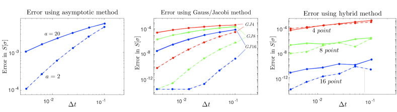
Figure 2: Comparison of quadrature methods for the single layer potential on a straight line segment with oscillatory density. For all panels, the dashed lines correspond to the case $k=10$ in (81), while the solid lines correspond to $k=100$.

As a final example, we consider a more general task: computation of the double layer potential $D[\mu]({\bf x},\Delta t)$ on a moving ellipse given by

$$\begin{cases}y_{1}(\theta,t)=20\cos(\theta)+1.5t,\\ y_{2}(\theta,t)=\sin(\theta),\end{cases}(0\leq\theta\leq 2\pi)$$ (82)

The density is chosen to be

$$\mu({\bf y},t)=\cos(y_{1}t)+\sin(10t).$$ (83)

We evaluate the double layer potential at ${\bf y}=(21.5,0.0)$ and $t=1.0$ using the same set of methods. Errors are plotted in Fig. 3.

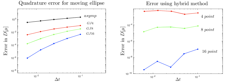
Figure 3: Comparison of quadrature methods for the double layer potential on a moving ellipse with oscillatory density given by (83).

5 Conclusions

We have developed a new method for the evaluation of layer heat potentials in two dimensions. By making use of an exponential change of variables, we overcome the phenomenon of “geometrically-induced stiffness,” which prevents the robust application of high order Gauss-Jacobi type quadrature rules. In our hybrid scheme, we combine a local asymptotic approximation with Gauss-Legendre quadrature in the transformed time variable. The corresponding spatial boundary integral operators involve only Gaussian kernels, permitting the application of the fast Gauss transform [20]. The scheme is easy to use with moving boundaries and precisely the same rule can be used in three dimensions with respect to the time variable. A full solver for the heat equation in fixed and moving geometries, incorporating the scheme of the present paper, will be described at a later date.

Appendix A Stirling’s formula, Cramer’s inequality and Gauss-Legendre quadrature

In the proof of Theorem 2 we make use of Stirling’s formula.

$$\sqrt{2\pi}\left(\frac{n}{e}\right)^{n}\sqrt{n}\leq n!\leq e\left(\frac{n}{e}\right)^{n}\sqrt{n}.$$ (84)

From this, it is staightforward to derive the following

Corollary 5.

Let $n\in{\bf N}$, we have:

$$\sqrt{(2n)!}\leq Cn^{1/4}(2n-1)!!\;\;,$$ (85)

where $C>0$ is a constant.

We also use Cramer’s inequality [11].

Lemma 5.

Let $h_{n}(t)$ be the $n-th$ order Hermite function, defined by

$$h_{n}(t)=(-1)^{n}D^{n}e^{-t^{2}}.$$ (86)

Then

$$|h_{n}(t)|\leq K2^{n/2}\sqrt{n!}e^{-t^{2}/2},$$ (87)

where $K$ is some constant with numerical value $K\leq 1.09$.

The following lemma is a direct consequence of Leibniz’s product rule for differentiation.

Lemma 6.

Let $F(t)=\frac{1}{t}$ and $f(t)=\frac{1}{\sqrt{t}}$. Then we have:

$$F^{(2n)}(t)=\sum_{k=0}^{2n}{2n\choose k}|f^{(2n-k)}(t)|\cdot|f^{(k)}(t)|.$$ (88)

Finally, we state the standard error estimate for Gauss-Legendre quadrature [4].

Lemma 7.

Let $f\in C^{2n}([a,b])$ and let $\{x_{1},\cdots,x_{n}\}$ and $\{w_{1},\cdots,w_{n}\}$ be the Gauss-Legendre nodes and weights scaled to $[a,b]$. If we denote the quadrature error by $E_{n}(f)$, we have:

$$\begin{split}E_{n}(f)&=\int_{a}^{b}f(x)dx-\sum_{k=1}^{n}w_{k}f(x_{k})\\ &=\frac{(b-a)^{2n+1}(n!)^{4}}{(2n+1)[(2n)!]^{3}}f^{(2n)}(\xi),\end{split}$$ (89)

where $\xi\in[a,b]$.

References

- [1] B. K. Alpert, Hybrid Gauss-trapezoidal quadrature rules, SIAM J. Sci. Comput., 20 (1999), pp. 1551–1584 (electronic).
- [2] K. E. Atkinson, The Numerical Solution of Integral Equations of the Second Kind, Cambridge University Press, New York, NY, 1997.
- [3] J. Bremer, V. Rokhlin, and I. Sammis, Universal quadratures for boundary integral equations on two-dimensional domains with corners, J. Comput. Phys., 229 (2010), pp. 8259–8280.
- [4] P. J. Davis and P. Rabinowitz, Methods of numerical integration, Academic Press, San Diego, 1984.
- [5] L. Greengard and J.-Y. Lee, Stable and accurate integral equation methods for scattering problems with multiple interfaces in two dimensions, J. Comput. Phys., 231 (2012), pp. 2389–2395.
- [6] L. Greengard and P. Lin, Spectral approximation of the free-space heat kernel, Appl. Comput. Harmon. Anal., 9 (2000), pp. 83–97.
- [7] Leslie Greengard and John Strain, A fast algorithm for the evaluation of heat potentials, Comm. Pure Appl. Math., 43 (1990), pp. 949–963.
- [8] , The fast Gauss transform, SIAM J. Sci. Statist. Comput., 12 (1991), pp. 79–94.
- [9] R. B. Guenther and J. W. Lee, Partial differential equations of mathematical physics and integral equations, Prentice Hall, Inglewood Cliffs, New Jersey, 1988.
- [10] J. Helsing and R. Ojala, Corner singularities for elliptic problems: integral equations, graded meshes, and compressed inverse preconditioning, J. Comput. Phys., 227 (2008), pp. 8820–8840.
- [11] E. Hille, A class of reciprocal functions, Annals of Mathematics: Second Series, 27 (1926), pp. 427–464.
- [12] Jing-Rebecca Li and Leslie Greengard, High order accurate methods for the evaluation of layer heat potentials, SIAM Journal on Scientific Computing, 31 (2009), pp. 3847–3860.
- [13] P. Lin, On the numerical solution of the heat equation in unbounded domains, PhD thesis, New York University, 1993.
- [14] W. Pogorzelski, Integral equations and their applications, Pergamon Press, Oxford, 1966.
- [15] R. S. Sampath, H. Sundar, and S. Veerapaneni, Parallel fast gauss transform, in SC ’10: Proceedings of the ACM/IEEE International Conference for High Performance Computing, Networking, Storage and Analysis, New Orleans, LA, 2010, pp. 1–10.
- [16] J. Strain, Fast adaptive methods for the free-space heat equation, SIAM J. Sci. Comput., 15 (1994), pp. 185–206.
- [17] J. Tausch, A fast method for solving the heat equation by layer potentials, J. Comput. Phys., (2007).
- [18] J. Tausch and A. Weckiewicz, Multidimensional fast Gauss transforms by Chebyshev expansions, SIAM J. Sci. Comput., 31 (2009), pp. 3547–3565.
- [19] L. N. Trefethen, Numerical computation of the schwarz-christoffel transformation, SIAM J. Sci. Stat. Comput., 1 (1980), pp. 82–102.
- [20] J. Wang and L. Greengard, An adaptive fast Gauss transform in two dimensions, SIAM J. Sci. Comput., to appear (arXiv:1712.00380) (2017).