Resummation for (boosted) top-quark pair production at NNLO+NNLL^′ in QCD

Abstract

We construct predictions for top quark pair differential distributions at hadron colliders that combine state-of-the-art NNLO QCD calculations with double resummation at NNLL^′ accuracy of threshold logarithms arising from soft gluon emissions and of small mass logarithms. This is the first time a resummed calculation at full NNLO+NNLL^′ accuracy in QCD for a process with non-trivial color structure has been completed at the differential level. Of main interest to us is the stability of the $M_{t\bar{t}}$ and top-quark $p_{T}$ distributions in the boosted regime where fixed order calculations may become strongly dependent on the choice of dynamic scales. With the help of numeric and analytic arguments we confirm that the choice for the factorization and renormalization scales advocated recently by some of the authors is indeed optimal. We further derive a set of optimized kinematics-dependent scales for the matching functions which appear in the resummed calculations. Our NNLO+NNLL^′ prediction for the top-pair invariant mass is significantly less sensitive to the choice of factorization scale than the fixed order prediction, even at NNLO. Notably, the resummed and fixed order calculations are in nearly perfect agreement with each other in the full $M_{t\bar{t}}$ range when the optimal dynamic scale is used. For the top-quark $p_{T}$ distribution the resummation performed here has less of an impact and instead we find that upgrading the matching with fixed-order from NLO+NNLL^′ to NNLO+NNLL^′ to be an important effect, a point to be kept in mind when using NLO-based Monte Carlo event generators to calculate this distribution.

1 Introduction

The top quark is the heaviest fundamental particle discovered so far. Because of its large mass, the top quark is the Standard Model particle which couples most strongly to the Higgs boson; as such, it plays a pivotal role in the study of the electroweak symmetry sector of the Standard Model. For this reason, and thanks to the large number of top-quark pairs produced at the Large Hadron Collider (LHC), accurate experimental measurements of several top-quark related observables are either already available or will become available in the next few years.

An exciting feature of top physics at the LHC is that the large collider energy enables the study of boosted top-quark production. In this context “boosted” refers to the kinematic regime where the energies of the produced top quarks are much larger than the top-quark mass. Boosted top quarks may appear in the study of many kinematic distributions: top quarks with very high pair invariant mass, top quarks with very large transverse momentum, or very forward top quarks (large rapidity). The LHC has already probed top quarks with transverse momenta around 1 TeV Aaboud:2018eqg , and will extend the energy range up to a few TeV. While these boosted energy top quarks are more rarely produced than the low energy ones, and the high energy regions do not contribute significantly to the total cross section, they are phenomenologically important due to their potential to probe directly physics beyond the electroweak scale.

On the theory side, state-of-the-art perturbative calculations for on-shell top-quark pair production, in the boosted regime or otherwise, have reached an accuracy beyond next-to-leading order (NLO) in the strong coupling constant $\alpha_{s}$. The most complete Standard Model predictions for differential cross sections combine next-to-next-leading-order (NNLO) QCD corrections with NLO electroweak (EW) ones Czakon:2017wor . In this paper we will focus exclusively on QCD corrections, with the understanding that the results can eventually be combined with EW corrections which have been studied extensively in the literature Beenakker:1993yr ; Kuhn:2005it ; Bernreuther:2005is ; Kuhn:2006vh ; Bernreuther:2006vg ; Hollik:2007sw ; Bernreuther:2008md ; Bernreuther:2010ny ; Denner:2010jp ; Bevilacqua:2010qb ; Hollik:2011ps ; Kuhn:2011ri ; Manohar:2012rs ; Bernreuther:2012sx ; Denner:2012yc ; Frederix:2013gra ; Kuhn:2013zoa ; Campbell:2016dks ; Pagani:2016caq ; Denner:2016jyo .

NNLO QCD calculations for differential cross sections in top-quark pair production were obtained in Czakon:2015owf ; Czakon:2016dgf . These calculations added to NNLO results for more inclusive quantities such as the total cross section Baernreuther:2012ws ; Czakon:2012zr ; Czakon:2012pz ; Czakon:2013goa and the forward-backward asymmetry at the Tevatron Czakon:2014xsa . In Czakon:2015owf , distributions such as the $t\bar{t}$ (top-pair) invariant mass and the top-quark transverse momentum distribution were evaluated at the LHC with center-of-mass energies of $\sqrt{s}=8$ TeV and 13 TeV using renormalization and factorization scales $\mu$ varied around the top mass $m_{t}$, and the typical scale uncertainties were estimated to lie below $10\%$. In Czakon:2016dgf , on the other hand, dynamical scale choices were investigated in order to determine which choice of scale is most appropriate for fixed-order studies of multi-TeV differential cross sections, based on the convergence of the fixed-order perturbative series. A notable result of that study is that the high-energy tails of distributions can be quite sensitive to the parametric choice of factorization scale, even at NNLO and especially in the case of the top-pair invariant mass distribution.

The fact that the application of fixed-order perturbation theory in the boosted regime is rather delicate is not entirely surprising. Indeed, in the case of boosted top quarks one encounters two potential difficulties. The first is that in the boosted regime the result of a fixed-order calculation contains mass logarithms of the form $\ln(E_{t}/m_{t})$ arising from quasi-collinear gluon emissions. The second is that, due to the shape of the parton distribution functions (PDFs), the effective partonic center-of-mass energies in most events with boosted top quarks are not much larger than the invariant masses of the top quark pairs. This can lead to enhanced corrections from so-called soft logarithms or threshold logarithms, and indeed, in general the two types of logarithms multiply each other at a given order in perturbation theory, due to emissions which are simultaneously soft and collinear. At the LHC, these logarithmic corrections may become important numerically, to the point that higher order corrections are not generically much smaller than lower order ones, and while it may be possible to deal with this to some extent through a judicious scale-setting procedure in a fixed-order calculation, it is desirable to address the issue head-on by resumming these two types of logarithms to all orders in perturbation theory and adding them onto the fixed order result through a matching procedure.

A framework for the simultaneous resummation of threshold and small-mass logarithms in differential cross sections in top-quark pair production at the LHC was set up in Ferroglia:2012ku , and applied to the phenomenological study of $t\bar{t}$ invariant mass and top-quark transverse momentum distributions in Pecjak:2016nee . The results are valid in the soft gluon emission limit, but contain an extra layer of resummation for small-mass logarithms, so that overlapping soft and small-mass logarithmic corrections are properly taken into account. The factorization formalism underlying the resummation was derived using soft-collinear effective theory (SCET), and the resummation was carried out in Mellin space. While the focus of that phenomenological study was the boosted regime, a matching procedure with standard soft-gluon resummation results (i.e. without the simultaneous resummation of small-mass logarithms) at next-to-next-to-leading logarithmic (NNLL) accuracy Ahrens:2010zv and to NLO fixed-order calculations was performed in order to expand the validity of the results to the full phase space.

In this paper we combine state-of-the-art results from analytic resummation and fixed-order perturbation theory in QCD in order to produce for the first time phenomenological predictions which match NNLO results with resummation of soft and small-mass logarithms at the level of differential $t\bar{t}$ invariant mass and top-quark transverse momentum distributions.

The paper is organized as follows. In section 2 we immediately address the technical aspect which is new in this work, namely the matching of the resummed calculation in the soft and boosted limit to the NNLO calculations. In section 3 we explain the resummation procedures used in two distinct kinematic limits. In particular, in section 3.1 we review the kinematics for top-pair production and the form of the differential cross section in Mellin space. In section 3.2 we discuss the soft limit, where threshold logarithms are large but mass logarithms are of generic size, while in section 3.3 we consider the boosted-soft limit, where both soft and mass logarithms are considered large. With all the analytic tools ready, in section 4 we study kinematic features of the top quark pair in the boosted region, and use these insights to determine appropriate choices for the scales appearing in the matching functions in the resummed formulas. In section 5 we present numerical results for the top-pair invariant mass and top-quark $p_{T}$ distributions, paying close attention to a comparison between pure NNLO results and those supplemented by resummation, and then present conclusions in section 6. We perform more comparisons among results at different orders in fixed-order and resummed perturbation theory in appendix A, and relegate some lengthy formulas for resummation exponents to appendix C.

2 Matching fixed order and resummed calculations

We study the top-quark pair production process

$$N_{1}(P_{1})+N_{2}(P_{2})\rightarrow t(p_{3})+\bar{t}(p_{4})+X(p_{X})\,,$$ (1)

where $N_{1}$ and $N_{2}$ are the colliding hadrons (proton-proton for the LHC and future colliders, proton-antiproton for the Tevatron), and $X$ is an inclusive hadronic final-state. In this work, the top quarks are treated as on-shell particles. QCD factorization allows us to write an arbitrary differential cross section in the schematic form

$$d\sigma=\sum_{i,j}\,d\hat{\sigma}_{ij}\otimes\phi_{i/N_{1}}\otimes\phi_{j/N_{2}}\,.$$ (2)

The symbol $\otimes$ stands for a convolution over longitudinal momentum fractions of the initial-state partons $i,j\in\{q,\bar{q},g\}$ in the (anti-)proton, the $d\hat{\sigma}_{ij}$ are the differential partonic cross sections for the process $i+j\to t\bar{t}+\hat{X}$, the $\hat{X}$ is a partonic final state, and $\phi_{i/N}$ denotes the parton distribution function (PDF) of parton $i$ in hadron $N$. While the PDFs are non-perturbative objects to be extracted from experiment, the differential partonic cross sections can be calculated in perturbative QCD.

The aim of this paper is to provide state-of-the-art QCD calculations for two specific differential cross sections: namely the invariant mass of the top-quark pair, and the $p_{T}$ of the top-quark. The baseline for the calculation is NNLO in fixed-order perturbation theory, to which we add the two types of resummation mentioned in the introduction and to be described in detail in section 3. The first is performed in the soft limit of the differential partonic cross sections, where the top-quark pair carries almost all of the energy of the partonic collision. It can be obtained to NNLL_m order using the results of Ahrens:2010zv , where we have labeled the logarithmic accuracy of the resummation with a subscript $m$ to indicate that the result is obtained for arbitrary values of $m_{t}$. As the energy of the top-quark pair becomes very large, this standard soft-gluon resummation itself develops logarithms which become large in the limit $m_{t}\to 0$. We call this the “boosted-soft limit”, and perform a joint resummation of overlapping soft and small-mass logarithms using the formalism developed in Ferroglia:2012ku . In this case it is possible to increase the accuracy of the resummation to NNLL${}^{\prime}_{b}$ order, where now the subscript $b$ indicates that the results are valid in the boosted-soft limit, and thus neglect corrections which vanish in the limit $m_{t}\to 0$. The perturbative ingredients for these two types of resummation (anomalous dimensions and matching functions) and the order at which they need to be calculated to achieve a given resummation accuracy is summarized in table 1 in section 3.4.

We have just described three different calculational formalisms, each of which is tailored to a different kinematic situation. The NNLO calculation is optimal in regions of phase space where the top quarks are not highly boosted, and hard-gluon emissions are important. The NNLL_m result is applicable when soft-gluon radiation dominates, but small-mass logarithms are unimportant. When soft-gluon radiation dominates, and the top-quarks are highly boosted, one would like to make use of the NNLL${}^{\prime}_{b}$ results. To make optimal use of our results we would like to have a unified description over the whole phase space. For this purpose it is necessary to combine the different formulas in such a way that no contribution is counted more than once.

To understand such a matching procedure, we first consider matching NNLL_m resummation with fixed-order results. In that case, the matching formula with (N)NLO reads

$$d\sigma^{\mathrm{(N)NLO+NNLL}_{m}}=d\sigma^{\mathrm{NNLL}_{m}}+\bigg{(}d\sigma^{\mathrm{(N)NLO}}-d\sigma^{\mathrm{NNLL}_{m}}\Big{|}_{\begin{subarray}{c}\text{(N)NLO}\\ \text{expansion}\end{subarray}}\bigg{)}\,,$$ (3)

where $d\sigma^{\mathrm{NNLL}_{m}}$ denotes the differential cross section evaluated to NNLL_m accuracy. The first term in the above equation contains the all-orders resummation result in the soft limit, and the difference of terms in parenthesis contains subleading terms in that limit, which are taken into account by the fixed-order calculation. Explicit expressions for the fixed-order (N)NLO expansion of the resummation formulas needed in the matching are given in section 3.6.

We next match the resummation formulas in the soft and boosted-soft limit with each other and with (N)NLO. To do so, we need to remove the overlap between the NNLL${}^{\prime}_{b}$ and NNLL_m results to all orders in $\alpha_{s}$. This is done by exploiting the fact that the boosted-soft resummation formula is the small-mass limit of the soft-gluon resummation formula at any fixed order in $\alpha_{s}$, so we must subtract out the leading term in the limit $m_{t}\to 0$ in order not to double count. The combined result, denoted $\mathrm{NNLL}^{\prime}_{b+m}$, is thus given by

$$d\sigma^{\mathrm{NNLL}^{\prime}_{b+m}}=d\sigma^{\mathrm{NNLL}^{\prime}_{b}}+\left(d\sigma^{\mathrm{NNLL}_{m}}-\left.d\sigma^{\mathrm{NNLL}_{m}}\right|_{m_{t}\to 0}\right),$$ (4)

where the terms in the parenthesis account for contributions which are suppressed by $m_{t}/M$ in the boosted-soft limit and thus not included in the NNLL${}^{\prime}_{b}$ result. Matching with fixed order then proceeds in analogy to eq. (3) resulting in

$$d\sigma^{\mathrm{(N)NLO+NNLL}^{\prime}}=d\sigma^{\mathrm{NNLL}^{\prime}_{b+m}}+\bigg{(}d\sigma^{\mathrm{(N)NLO}}-\left.d\sigma^{\mathrm{NNLL}^{\prime}_{b+m}}\right|_{\begin{subarray}{c}\mathrm{(N)NLO}\\ \mathrm{expansion}\end{subarray}}\bigg{)}\,.$$ (5)

Again, the terms in the parenthesis account for subleading terms in the soft limit, which are taken into account through a fixed-order calculation, but are not accessible to either of the resummation formulas. Calculating the subtraction term requires one to expand each term in eq. (4) to (N)NLO. The procedure for obtaining the different components of the above equation is described in more detail in section 3.6.

Differential distributions obtained from the explicit evaluation of eq. (5) are a main result of this work, and can be found in section 5. Before going into numerical studies, we give details of the resummation procedure, including recipes for obtaining the different pieces used in the matching procedure, in the next section. These details can safely be skipped by a reader interested in purely phenomenological results. In section 4 we conduct a thorough analysis of the choice of scales for the matching functions which appear in the resummed results.

3 Mellin-space resummation in the (boosted) soft limit

3.1 Kinematics and differential cross sections

In this section we review the kinematics involved in describing the limits in which resummation is carried out. At Born level, and to leading order in the soft limit considered below, two partonic channels contribute to the partonic cross section: the quark-antiquark annihilation channel

$$q(p_{1})+\bar{q}(p_{2})\rightarrow t(p_{3})+\bar{t}(p_{4})\,,$$ (6)

and the gluon fusion channel

$$g(p_{1})+g(p_{2})\rightarrow t(p_{3})+\bar{t}(p_{4})\,.$$ (7)

The momenta of the incoming partons are related to the hadron momenta according to ${p_{i}=x_{i}P_{i}}$ ($i=1,2$). The relevant Mandelstam invariants are defined as

$$s=(P_{1}+P_{2})^{2}\,,\quad\hat{s}=(p_{1}+p_{2})^{2}\,,\quad M_{t\bar{t}}^{2}=(p_{3}+p_{4})^{2}\,,$$

$$t_{1}=(p_{1}-p_{3})^{2}-m_{t}^{2}\,,\quad u_{1}=(p_{2}-p_{3})^{2}-m_{t}^{2}\,.$$ (8)

In fixed order perturbation theory, starting from NLO accuracy, a new $2\to 3$ production channel, initiated by a quark and a gluon, opens up. At NNLO one needs to account for the contribution of $2\to 4$ processes (at tree level), as well as the contribution of $2\to 3$ processes (up to one loop) and the $2\to 2$ production channels in eqs. (6) and (7) (up to two-loops). All of these channels are of course included in the NNLO results which we employ in this work.

The soft emission region, which is of interest for the resummed calculation, is defined by the limit $M_{t\bar{t}}^{2}\to\hat{s}$ (sometimes also referred to as the partonic threshold region). In this limit, the final state particles in addition to the top pair are soft. In order to describe the top-pair invariant mass distribution near the partonic threshold, it is convenient to introduce the following variables:

$$z=\frac{M_{t\bar{t}}^{2}}{\hat{s}}\,,\quad\tau=\frac{M_{t\bar{t}}^{2}}{s}\,,\quad\beta_{t}=\sqrt{1-\frac{4m_{t}^{2}}{M_{t\bar{t}}^{2}}}\,,\quad\beta=\sqrt{1-\frac{4m_{t}^{2}}{\hat{s}}}\,.$$ (9)

The quantity $\beta_{t}$ is the 3-velocity of the (anti-)top quark in the $t\bar{t}$ rest frame, while $\beta$ is often invoked to describe the partonic threshold for the total cross section Bonciani:1998vc ; Czakon:2009zw ; Beneke:2011mq ; Beneke:2010da . In the soft limit $z\to 1$, one has $\beta\to\beta_{t}$. Moreover, in that limit the scattering angle $\theta$ is related to the Mandelstam variables according to

$$t_{1}=-\frac{M_{t\bar{t}}^{2}}{2}(1-\beta_{t}\cos\theta)\,,\quad u_{1}=-\frac{M_{t\bar{t}}^{2}}{2}(1+\beta_{t}\cos\theta)\,,$$ (10)

from which one can easily verify the usual relation $M_{t\bar{t}}^{2}+t_{1}+u_{1}=0$.

We will perform resummation on the double differential cross section in the top-pair invariant mass and the scattering angle $\theta$. Applying the generic QCD factorization formula eq. (2) allows one to write this differential cross section as

$$\frac{d^{2}\sigma(\tau)}{dM_{t\bar{t}}\,d\cos\theta}=\frac{8\pi\beta_{t}}{3sM_{t\bar{t}}}\sum\limits_{ij}\int^{1}_{\tau}\frac{dz}{z}\,\mathcal{L}_{ij}(\tau/z,\mu_{f})\,C_{ij}(z,M_{t\bar{t}},m_{t},\cos\theta,\mu_{f})\,,$$ (11)

where $M_{t\bar{t}}$ and $\cos\theta$ are in the ranges

$$2m_{t}\leq M_{t\bar{t}}\leq s\,,\quad|\cos\theta|\leq 1\,.$$ (12)

The hard-scattering kernels $C_{ij}$ are proportional to the partonic cross sections and can be calculated in perturbation theory at the factorization scale $\mu_{f}$, while $\mathcal{L}_{ij}$ are non-perturbative parton luminosity functions, defined as

$$\mathcal{L}_{ij}(y,\mu_{f})=\int_{y}^{1}\frac{dx}{x}\,\phi_{i/N_{1}}(x,\mu_{f})\,\phi_{j/N_{2}}(y/x,\mu_{f})\,.$$ (13)

In this work, we study the resummation in two limits where soft and collinear gluon emissions dynamically generate scales much lower than the scattering energy:

soft limit: $$\quad\hat{s},|t_{1}|,m_{t}^{2}\gg\hat{s}(1-z)^{2}\,,$$ (14)

boosted-soft limit: $$\quad\hat{s},|t_{1}|\gg m_{t}^{2}\gg\hat{s}(1-z)^{2}\gg m_{t}^{2}(1-z)^{2}\,.$$ (15)

In each of these limits the perturbative expansions of the hard-scattering kernels contain large logarithms of scale ratios, which can be resummed to all orders in $\alpha_{s}$. For the discussion of resummation that follows, it is convenient to study the cross section in Laplace or Mellin space. The Mellin transform and its inverse are defined by

$$\tilde{f}(N)=\mathcal{M}[f](N)=\int_{0}^{1}dx\,x^{N-1}{f}(x)\,,\quad f(x)=\mathcal{M}^{-1}[\tilde{f}](x)=\frac{1}{2\pi i}\int_{c-i\infty}^{c+i\infty}dN\,x^{-N}\tilde{f}(N),$$ (16)

where in the inverse transform the real part of the contour $c$ is chosen such that it lies to the right of all singularities in the function $\tilde{f}(N)$. Convolutions such as the differential cross section in eq. (11) become simple products in Mellin space. Indeed, by performing the Mellin transform of eq. (11) with respect to $\tau$, we find the differential cross section in Mellin space, which reads

$$\frac{d^{2}\widetilde{\sigma}(N)}{dM_{t\bar{t}}\,d\cos\theta}=\frac{8\pi\beta_{t}}{3sM_{t\bar{t}}}\sum_{ij}\widetilde{\mathcal{L}}_{ij}(N,\mu_{f})\,\widetilde{c}_{ij}(N,M_{t\bar{t}},m_{t},\cos\theta,\mu_{f})\,.$$ (17)

The soft limit $z\to 1$ corresponds to $N\to\infty$, as can be seen by taking the Mellin transform of the plus distributions appearing in the partonic cross section, which are generated by soft gluon emissions:

$$\mathcal{M}[P_{0}](N) =-\ln{\bar{N}}+\mathcal{O}\left(\frac{1}{N}\right)\ ,$$

$$\mathcal{M}[P_{1}](N) =\frac{1}{2}\left(\ln^{2}{\bar{N}}+\frac{\pi^{2}}{6}\right)+\mathcal{O}\left(\frac{1}{N}\right)\ ,$$

$$\mathcal{M}[P_{2}](N) =-\frac{1}{3}\left(\ln^{3}{\bar{N}}+\frac{\pi^{2}}{2}\ln{\bar{N}}+2\zeta(3)\right)+\mathcal{O}\left(\frac{1}{N}\right)\ ,$$

$$\mathcal{M}[P_{3}](N) =\frac{1}{4}\left(\ln^{4}{\bar{N}}+\pi^{2}\ln^{2}{\bar{N}}+8\zeta(3)\ln{\bar{N}}+\frac{3\pi^{4}}{20}\right)+\mathcal{O}\left(\frac{1}{N}\right)\ ,$$ (18)

where

$$P_{n}(z)=\left[\frac{\ln^{n}(1-z)}{1-z}\right]_{+}\,,$$ (19)

and we have introduced the variable $\bar{N}=Ne^{\gamma_{E}}$ in order to simplify the expressions, with $\gamma_{E}$ denoting the Euler constant. We note that the partonic cross section contains terms of the form $\alpha_{s}^{n}P_{k}(z)$ where $0\leq k\leq 2n-1$ at NⁿLO in its perturbative expansion. In Mellin space this becomes $\alpha_{s}^{n}L^{k}$ where $L=\ln\bar{N}$ and $0\leq k\leq 2n$, which will be important when we consider the tower of logarithms which can be resummed in section 3.4. In Mellin moment space, the soft and boosted-soft limits in eqs. (14) and (15) become

Mellin-space soft limit: $$\quad\hat{s},|t_{1}|,m_{t}^{2}\gg\frac{\hat{s}}{N^{2}}\,,$$ (20)

Mellin-space boosted-soft limit: $$\quad\hat{s},|t_{1}|\gg m_{t}^{2}\gg\frac{\hat{s}}{N^{2}}\gg\frac{m_{t}^{2}}{N^{2}}\,.$$ (21)

Besides the invariant mass distribution, the distribution in the transverse momentum $p_{T}$ of the top quark is also interesting. In Ferroglia:2013awa , a different formulation, dubbed “1PI”, was employed to deal with such “single-particle-inclusive” observables in the boosted regime. In contrast, the formulation used in this paper was called “pair-invariant-mass” (PIM) kinematics. Near the partonic threshold, the PIM and 1PI formulations differ only by power-suppressed contributions. We can exploit this fact to express the differential cross section with respect to $p_{T}$ in terms of the double differential cross section in eq. (11), thereby avoiding the introduction of the 1PI formulation. In the threshold limit, the transverse momentum $p_{T}$ and the rapidity $\hat{y}$ of the top-quark in the partonic center-of-mass frame are given by

$$p_{T}=\frac{M_{t\bar{t}}\beta_{t}}{2}\sin\theta\,,\quad\hat{y}=\frac{1}{2}\ln\frac{1+\beta_{t}\cos\theta}{1-\beta_{t}\cos\theta}\,,$$ (22)

and we can write the differential cross section with respect to $p_{T}$ and $\hat{y}$ in Mellin space as

$$\frac{d^{2}\widetilde{\sigma}(N)}{dp_{T}\,d\hat{y}}=2\sin\theta\,\frac{d^{2}\widetilde{\sigma}(N)}{dM_{t\bar{t}}\,d\cos\theta}=\frac{16\pi\beta_{t}\sin\theta}{3sM_{t\bar{t}}}\sum_{ij}\widetilde{\mathcal{L}}_{ij}(N,\mu_{f})\,\widetilde{c}_{ij}(N,M_{t\bar{t}},m_{t},\cos\theta,\mu_{f})\,.$$ (23)

In the above equation, it is understood that $M_{t\bar{t}}$ and $\cos\theta$ should be expressed in terms of the integration variables according to

$$M_{t\bar{t}}=2m_{T}\cosh(\hat{y})\equiv 2\sqrt{p_{T}^{2}+m_{t}^{2}}\cosh(\hat{y})\,,\quad\cos\theta=\frac{1}{\beta_{t}}\,\tanh(\hat{y})\,,$$ (24)

where we have defined the transverse mass $m_{T}$. The transverse momentum distribution can be obtained by integrating over $\hat{y}$ in the range

$$|\hat{y}|\leq\mathrm{arccosh}\left(\frac{\sqrt{s}}{2m_{T}}\right),$$ (25)

while the range of $p_{T}$ is

$$0\leq p_{T}\leq\sqrt{\frac{s}{4}-m_{t}^{2}}\,.$$ (26)

3.2 Resummation in the soft limit

Resummation of top-quark hadroproduction cross sections in the partonic threshold limit $z\to 1$ was considered in Kidonakis:1997gm . More recently, top-pair production in the soft limit was re-analyzed by means of SCET methods. With this technique, it was possible to study the resummation of soft gluon emission corrections both in PIM and 1PI kinematics Ahrens:2010zv ; Ahrens:2011mw in momentum space. Here we follow closely the discussion and notation of the NNLL calculation of Ahrens:2010zv , although we perform the resummation in Mellin rather than momentum space. This approach was adopted in Pecjak:2016nee for top-pair production. Subsequently, it was also applied to the evaluation of the soft emission corrections to $t\bar{t}W^{\pm}$ Broggio:2016zgg , $t\bar{t}H$ Broggio:2016lfj , and $t\bar{t}Z$ Broggio:2017kzi to NNLL accuracy. The starting point is the factorization of the partonic cross section in the soft limit. In Mellin space, this takes the form

$$\widetilde{c}_{ij}(N,M_{t\bar{t}},m_{t},\cos\theta,\mu_{f})=\mathrm{Tr}\Bigg{[}\bm{H}^{m}_{ij}(M_{t\bar{t}},m_{t},\cos\theta,\mu_{f})\\ \times\widetilde{\bm{s}}^{m}_{ij}\left(\ln\frac{M_{t\bar{t}}^{2}}{\bar{N}^{2}\mu_{f}^{2}},M_{t\bar{t}},m_{t},\cos\theta,\mu_{f}\right)\Bigg{]}+\mathcal{O}\left(\frac{1}{N}\right).$$ (27)

The hard functions $\bm{H}^{m}_{ij}$ and the soft functions $\widetilde{\bm{s}}^{m}_{ij}$, referred to generically as matching functions, are matrices in color space — explicit results for the two-by-two matrices in the $q\bar{q}$ channel and three-by-three matrices in the $gg$ channel up to NLO in $\alpha_{s}$ can be extracted from Ahrens:2010zv , where the derivation of a momentum-space factorization formula analogous to eq. (27) is given in detail. Comparing to the notation employed in Ahrens:2010zv , here we have introduced a superscript $m$ on these functions, indicating that they contain full dependence on the top quark mass $m_{t}$. This is to distinguish them from the corresponding functions with $m_{t}=0$ used later in the boosted-soft limit.

Given the factorized form of the partonic cross section in Mellin space, one can derive and solve renormalization group (RG) equations for the component functions. This allows one to evaluate the hard and soft functions at an arbitrary hard scale $\mu_{h}$ and soft scale $\mu_{s}$, where large logarithms are absent. One then uses RG evolution to obtain the hard scattering kernels at the factorization scale $\mu_{f}$. These RG-improved hard-scattering kernels can be written as

$$\widetilde{c}_{ij}(N,\mu_{f})=\mathrm{Tr}\Bigg{[}\widetilde{\bm{U}}^{m}_{ij}(\!\bar{N},\mu_{f},\mu_{h},\mu_{s})\,\bm{H}^{m}_{ij}(\mu_{h})\,\widetilde{\bm{U}}_{ij}^{m\dagger}(\!\bar{N},\mu_{f},\mu_{h},\mu_{s})\widetilde{\bm{s}}^{m}_{ij}\left(\ln\frac{M_{t\bar{t}}^{2}}{\bar{N}^{2}\mu_{s}^{2}},\mu_{s}\right)\!\!\Bigg{]}\\ +\mathcal{O}\left(\!\frac{1}{N}\!\right),$$ (28)

where we have suppressed the dependence of all functions in eq. (28) on the variables $M_{t\bar{t}}$, $m_{t}$ and $\cos\theta$. The evolution matrices $\widetilde{\bm{U}}^{m}_{ij}$ contain all large logarithms in an exponentiated form, and thereby resum them to all orders in $\alpha_{s}$. The explicit form of the evolution matrices was derived in Ahrens:2010zv , and in Mellin space reads (suppressing for the moment the subscript $ij$ and the argument $\bar{N}$)

$$\widetilde{\bm{U}}^{m}(\mu_{f},\mu_{h},\mu_{s})=\exp\bigg{\{}2S_{\Gamma_{\text{cusp}}}(\mu_{h},\mu_{s})-a_{\Gamma_{\text{cusp}}}(\mu_{h},\mu_{s})\left(\ln\frac{M_{t\bar{t}}^{2}}{\mu_{h}^{2}}-i\pi\right)\\ +a_{\Gamma_{\text{cusp}}}(\mu_{f},\mu_{s})\ln\bar{N}^{2}+2a_{\gamma^{\phi}}(\mu_{s},\mu_{f})\bigg{\}}\\ \times\bm{u}^{m}(M_{t\bar{t}},m_{t},\cos\theta,\mu_{h},\mu_{s})\,.$$ (29)

The explicit exponential in the above equation is color-diagonal, and contains the evolution functions

$$S_{\gamma}(\nu,\mu)=-\int^{\alpha_{s}(\mu)}_{\alpha_{s}(\nu)}d\alpha\,\frac{\gamma(\alpha)}{\beta(\alpha)}\int^{\alpha}_{\alpha_{s}(\nu)}\frac{d\alpha^{\prime}}{\beta(\alpha^{\prime})}\,,\quad a_{\gamma}(\nu,\mu)=-\int^{\alpha_{s}(\mu)}_{\alpha_{s}(\nu)}d\alpha\frac{\gamma(\alpha)}{\beta(\alpha)}\,,$$ (30)

where $\gamma$ stands for an anomalous dimension such as $\Gamma_{\rm cusp}$ or $\gamma^{\phi}$, and $\beta(\alpha_{s})=d\alpha_{s}(\mu)/d\ln\mu$ is the QCD $\beta$-function. The matrix $\bm{u}^{m}$ in the second line of eq. (29) is given by

$$\bm{u}^{m}(M_{t\bar{t}},m_{t},\cos\theta,\mu_{h},\mu_{s})=\mathcal{P}\exp\int^{\alpha_{s}(\mu_{s})}_{\alpha_{s}(\mu_{h})}\frac{d\alpha}{\beta(\alpha)}\,\bm{\gamma}^{h,m}(M_{t\bar{t}},m_{t},\cos\theta,\alpha)\,,$$ (31)

where $\bm{\gamma}^{h,m}$ is the color non-diagonal part of hard anomalous dimension with full mass dependence, and $\mathcal{P}$ denotes path-ordering. The definition and the explicit expressions for the various anomalous dimensions can be readily found in the appendix of Ahrens:2010zv . Although we have dropped indices indicating the partonic channel in eqs. (29) and (31), one should keep in mind that the anomalous dimension $\gamma^{\phi}$, (related to the PDFs), the cusp anomalous dimensions $\Gamma_{\rm cusp}$, and the non-color diagonal anomalous dimension $\bm{\gamma}^{h,m}$ are different in the quark-annihilation and gluon fusion channels.

The above integrals appearing in the evolution matrices can be evaluated and truncated to a given logarithmic order. The results can be expressed in terms of the strong coupling constant evaluated at the various scales, $\alpha_{s}(\mu_{f})$, $\alpha_{s}(\mu_{h})$ and $\alpha_{s}(\mu_{s})$, as was done in Ahrens:2010zv . This is convenient if the soft scale $\mu_{s}$ is chosen directly in momentum space, and is thus a real number. However, in the current paper, we employ a more conventional choice of the soft scale in Mellin space, $\mu_{s}\sim\Lambda/\bar{N}$ for some mass scale $\Lambda$, which is now a complex number. It is therefore more convenient to re-express $\alpha_{s}(\mu_{s})$ in terms of $\alpha_{s}(\mu_{h})$, keeping in mind that $\ln(\mu_{h}/\mu_{s})$ is a large logarithm. Actually, it is conventional to express all $\alpha_{s}(\mu_{i})$ in terms of $\alpha_{s}(\mu_{h})$, where $\mu_{i}$ is any scale other than $\mu_{h}$ appearing in the formula. This can be done by using the perturbative evolution of the strong coupling, which up to 3-loop order is given by (see, e.g. Moch:2005ba )

$$\alpha_{s}(\mu)=\frac{\alpha_{s}(\mu_{h})}{X}\Bigg{[}1-\frac{\alpha_{s}(\mu_{h})}{4\pi}\,\frac{\beta_{1}}{\beta_{0}}\,\frac{\ln X}{X}\\ +\left(\frac{\alpha_{s}(\mu_{h})}{4\pi}\right)^{2}\frac{1}{X^{2}}\left[\frac{\beta_{1}^{2}}{\beta_{0}^{2}}\left(\ln^{2}X-\ln X-1+X\right)+\frac{\beta_{2}}{\beta_{0}}(1-X)\right]+{\cal O}(\alpha_{s}^{3}(\mu_{h}))\Bigg{]}\,,$$ (32)

where

$$X=1-\frac{\alpha_{s}(\mu_{h})}{2\pi}\beta_{0}\ln\frac{\mu_{h}}{\mu}\,.$$ (33)

Logarithmic orders are then determined according to powers of $\alpha_{s}(\mu_{h})$ with $\ln(\mu_{h}/\mu_{i})$ counted as order $1/\alpha_{s}(\mu_{h})$. For this reason we introduce two ${\cal O}(1)$ parameters: $\lambda_{s}$ and $\lambda_{f}$ defined by

$$\lambda_{i}=\frac{\alpha_{s}(\mu_{h})}{2\pi}\beta_{0}\ln\frac{\mu_{h}}{\mu_{i}}\,,$$ (34)

for $i=\{s,f\}$. The part of the exponent proportional to the identity matrix in eq. (29) can now be expanded as a series in $\alpha_{s}(\mu_{h})$, and the resulting evolution matrix can be written in the form

$$\widetilde{\bm{U}}^{m}(\mu_{f},\mu_{h},\mu_{s})=\exp\left\{\frac{4\pi}{\alpha_{s}(\mu_{h})}\,g^{m}_{1}(\lambda_{s},\lambda_{f})+g^{m}_{2}(\lambda_{s},\lambda_{f})+\frac{\alpha_{s}(\mu_{h})}{4\pi}\,g^{m}_{3}(\lambda_{s},\lambda_{f})+\cdots\right\}\\ \times\bm{u}^{m}(M_{t\bar{t}},m_{t},\cos\theta,\mu_{h},\mu_{s})\,.$$ (35)

Explicit expressions for the RG exponents $g_{i}^{m}$ are given in appendix C.1, while a method for evaluating $\bm{u}^{m}$ is detailed in Ahrens:2010zv using techniques from Buras:1991jm .

The all-order resummed hard scattering kernel eq. (28) is formally independent of the matching scales $\mu_{s}$ and $\mu_{h}$. However, the truncation of the resummed formula to a given logarithmic order introduces residual dependence on these scales. In order to perform the resummation, one must choose these scales in such a way that the fixed-order expansion of the hard and soft functions are free of large logarithms. The explicit form of the one-loop hard and soft functions reveals that the leading logarithmic terms are $\alpha_{s}\ln^{2}(M_{t\bar{t}}^{2}/\mu_{h}^{2})$ and $\alpha_{s}\ln^{2}(M_{t\bar{t}}^{2}/\bar{N}^{2}/\mu_{s}^{2})$, respectively, which motivates the naïve choices $\mu_{h}\sim M_{t\bar{t}}$ and $\mu_{s}\sim M_{t\bar{t}}/\bar{N}$. However, we will study the analytic form of the hard and soft functions in greater detail in section 4 in order to make a more informed choice of appropriate scales. It should be noted however, that in picking the soft scale $\mu_{s}$ directly in Mellin space (as we do in this work) the resummed hard-scattering kernel contains a branch cut at large $N$ due to the Landau pole in the running of $\alpha_{s}$. This leads to ambiguities in the choice of contour for the inverse Mellin transform in eq. (16). We come back to this issue when discussing the numerical implementation of our results in section 3.5. As mentioned earlier, one could also choose the soft scale directly in momentum space, which is then independent of $N$, as was done in Ahrens:2010zv . With this choice the inverse Mellin (or Laplace) transform for the soft function can be carried out analytically and is free from the Landau pole problem. On the other hand, this comes at the price of resumming a different tower of logarithms compared to the pure partonic threshold ones, as discussed in Ahrens:2011mw and explored in more detail in, e.g. Bonvini:2012az ; Bonvini:2014qga .

3.3 Resummation in the boosted-soft limit

Resummation of top-quark hadroproduction cross sections in the boosted-soft limit eq. (15) was considered in Ferroglia:2012ku . We first collect the main results from that paper in the absence of perturbative corrections involving closed top-quark loops. In that case, the functions $\bm{H}^{m}_{ij}$ and $\widetilde{\bm{s}}_{ij}^{m}$ in eq. (27) can be subfactorized in the $m_{t}\to 0$ limit as

$$\bm{H}^{m}_{ij}(M_{t\bar{t}},m_{t},\cos\theta,\mu_{f}) =\bm{H}_{ij}(M_{t\bar{t}},\cos\theta,\mu_{f})\,C_{D}^{2}(m_{t},\mu_{f})+\mathcal{O}\left(\frac{m_{t}}{M_{t\bar{t}}}\right),$$ (36)

$$\widetilde{\bm{s}}^{m}_{ij}\left(\ln\frac{M_{t\bar{t}}^{2}}{\bar{N}^{2}\mu_{f}^{2}},M_{t\bar{t}},m_{t},\cos\theta,\mu_{f}\right) =\widetilde{\bm{s}}_{ij}\left(\ln\frac{M_{t\bar{t}}^{2}}{\bar{N}^{2}\mu_{f}^{2}},M_{t\bar{t}},\cos\theta,\mu_{f}\right)\,\widetilde{s}_{D}^{2}\left(\ln\frac{m_{t}}{\bar{N}\mu_{f}},\mu_{f}\right)$$

$$\hskip 140.00021pt+\mathcal{O}\left(\frac{m_{t}}{M_{t\bar{t}}}\right).$$ (37)

In the above formulas, the hard functions $\bm{H}_{ij}$ and soft functions $\widetilde{\bm{s}}_{ij}$ without the superscript $m$ are independent of the top-quark mass $m_{t}$. They were calculated to NNLO in Broggio:2014hoa and Ferroglia:2012uy , respectively, and can also be applied to di-jet production. All $m_{t}$-dependence is factorized into the two functions $C_{D}$ and $\widetilde{s}_{D}$, which are related to the perturbative heavy-quark fragmentation function Melnikov:2004bm and were extracted at NNLO in Ferroglia:2012ku . After this refactorization, the result for the partonic cross section in the boosted-soft limit reads

$$\widetilde{c}_{ij}(N,M_{t\bar{t}},m_{t},\cos\theta,\mu_{f})=\mathrm{Tr}\left[\bm{H}_{ij}(M_{t\bar{t}},\cos\theta,\mu_{f})\,\widetilde{\bm{s}}_{ij}\Biggl{(}\ln\frac{M_{t\bar{t}}^{2}}{\bar{N}^{2}\mu_{f}^{2}},M_{t\bar{t}},\cos\theta,\mu_{f}\Biggr{)}\right]\\ \times C_{D}^{2}(m_{t},\mu_{f})\,\widetilde{s}_{D}^{2}\Biggl{(}\ln\frac{m_{t}}{\bar{N}\mu_{f}},\mu_{f}\Biggr{)}+\mathcal{O}\left(\frac{1}{N}\right)+\mathcal{O}\left(\frac{m_{t}}{M_{t\bar{t}}}\right).$$ (38)

As for the soft limit, the resummed hard-scattering kernel can be obtained by deriving and solving RG equations for the component functions in the above factorization formula. We write the result in the form

$$\widetilde{c}_{ij}(N,\mu_{f})=\mathrm{Tr}\Bigg{[}\widetilde{\bm{U}}_{ij}(\bar{N},\mu_{f},\mu_{h},\mu_{s})\,\bm{H}_{ij}(\mu_{h})\,\widetilde{\bm{U}}_{ij}^{\dagger}(\bar{N},\mu_{f},\mu_{h},\mu_{s})\widetilde{\bm{s}}_{ij}\left(\ln\frac{M_{t\bar{t}}^{2}}{\bar{N}^{2}\mu_{s}^{2}},\mu_{s}\right)\Bigg{]}\\ \times\,\widetilde{U}_{D}^{2}(\bar{N},\mu_{f},\mu_{dh},\mu_{ds})\,C_{D}^{2}(m_{t},\mu_{dh})\,\widetilde{s}_{D}^{2}\Biggl{(}\ln\frac{m_{t}}{\bar{N}\mu_{ds}},\mu_{ds}\Biggr{)}+\mathcal{O}\left(\frac{1}{N}\right)+\mathcal{O}\left(\frac{m_{t}}{M_{t\bar{t}}}\right).$$ (39)

In the l.h.s. of eq. (39) we dropped the dependence on the arguments $M_{t\bar{t}}$, $\cos\theta$ and $m_{t}$. Similarly, $\widetilde{\bm{U}}_{ij}$, $\bm{H}_{ij}$ and $\widetilde{\bm{s}}_{ij}$ also depend on $M_{t\bar{t}}$ and $\cos\theta$.

As mentioned with the massive hard and soft functions, we postpone discussion of the most appropriate scale choices for the matching functions $\bm{H}_{ij}$ and $\widetilde{\bm{s}}_{ij}$ until section 4. However, since the functions $C_{D}$ and $\widetilde{s}_{D}$ depend only on the scales $m_{t}$ and $m_{t}/\bar{N}$, we can immediately make the assignment $\mu_{dh}=m_{t}$ and $\mu_{ds}=m_{t}/\bar{N}$. The evolution of the hard and soft functions is encoded in the functions $\widetilde{\bm{U}}_{ij}$, which are matrices in color space, while the evolution of $C_{D}$ and $\widetilde{s}_{D}$ is in the color-diagonal function $\widetilde{U}_{D}$. Suppressing for the moment the channel labels $ij$, the explicit expressions for the evolution matrices are given by

$$\widetilde{\bm{U}}(\mu_{f},\mu_{h},\mu_{s}) =\exp\bigg{\{}2S_{A}(\mu_{h},\mu_{s})-a_{A}(\mu_{h},\mu_{s})\left(\ln\frac{M_{t\bar{t}}^{2}}{\mu_{h}^{2}}-i\pi\right)+a_{A}(\mu_{f},\mu_{s})\ln\bar{N}^{2}$$

$$\hskip 60.00009pt+2a_{\gamma^{\phi}}(\mu_{s},\mu_{f})+2a_{\gamma^{\phi_{q}}}(\mu_{s},\mu_{f})\bigg{\}}\,\bm{u}(M_{t\bar{t}},\cos\theta,\mu_{h},\mu_{s})\,,$$ (40)

$$\widetilde{U}_{D}(\mu_{f},\mu_{dh},\mu_{ds}) =\exp\bigg{\{}-2S_{\Gamma^{q}}(\mu_{dh},\mu_{ds})+a_{\Gamma^{q}}(\mu_{dh},\mu_{ds})\ln\frac{m_{t}^{2}}{\mu_{dh}^{2}}-a_{\Gamma^{q}}(\mu_{f},\mu_{ds})\ln\bar{N}^{2}$$

$$\hskip 60.00009pt-2a_{\gamma^{S}}(\mu_{dh},\mu_{ds})-2a_{\gamma^{\phi_{q}}}(\mu_{dh},\mu_{f})\bigg{\}}\,.$$ (41)

The functions $S_{A}$, $a_{\gamma}$, and $\bm{u}$ are defined analogously to those in eqs. (30) and (31). Here $A$ is given by $2\Gamma_{\rm cusp}^{q}$ in the $q\bar{q}$ channel and $\Gamma_{\rm cusp}^{q}+\Gamma_{\rm cusp}^{g}$ in the $gg$ channel. Definitions of the various anomalous dimensions and their explicit perturbative expansions can be found in Ferroglia:2012ku . In order to write the perturbative expansion of the evolution functions in the same form as eq. (35) we introduce two additional $\mathcal{O}(1)$ parameters, $\lambda_{dh}$ and $\lambda_{ds}$ in complete analogy to $\lambda_{s}$ and $\lambda_{f}$, as defined earlier in eq. (34). Following the same procedure as in the soft limit, the evolution matrices can then be written as

$$\widetilde{\bm{U}}(\mu_{f},\mu_{h},\mu_{s})= \exp\left\{\frac{4\pi}{\alpha_{s}(\mu_{h})}\,g_{1}(\lambda_{s},\lambda_{f})+g_{2}(\lambda_{s},\lambda_{f})+\frac{\alpha_{s}(\mu_{h})}{4\pi}\,g_{3}(\lambda_{s},\lambda_{f})\right\}$$

$$\times\bm{u}(M_{t\bar{t}},\cos\theta,\mu_{h},\mu_{s})\,,$$ (42)

and

$$U_{D}(\mu_{f},\mu_{dh},\mu_{ds})=\exp\bigg{\{} \frac{4\pi}{\alpha_{s}(\mu_{h})}\,g^{D}_{1}(\lambda_{dh},\lambda_{ds},\lambda_{f})+g^{D}_{2}(\lambda_{dh},\lambda_{ds},\lambda_{f})$$

$$+\frac{\alpha_{s}(\mu_{h})}{4\pi}\,g^{D}_{3}(\lambda_{dh},\lambda_{ds},\lambda_{f})\bigg{\}}\,.$$ (43)

We list the (lengthy) expressions for the RG-exponents $g_{i}$ and $g^{D}_{i}$ in appendix C.2.

In the presence of heavy-quark loops the factorization of the partonic cross section in the boosted-soft limit is more involved. It is necessary to introduce additional coefficients related to matching six-flavor PDFs, heavy-quark fragmentation functions, and $\alpha_{s}$ onto five-flavor ones. To ease notation we cluster these contributions from heavy quarks together in coefficients $\tilde{c}^{ij}_{t}$. Such corrections are proportional to powers of $n_{h}$, the number of heavy flavors, and introduce additional $m_{t}$ dependence into the formula via logarithms of the form $\ln^{n}(m_{t}/M_{t\bar{t}})$. Our factorized hard scattering kernel is then written as

$$\widetilde{c}_{ij}(N,M_{t\bar{t}},m_{t},\cos\theta,\mu_{f})=\mathrm{Tr}\left[\bm{H}_{ij}(M_{t\bar{t}},\cos\theta,\mu_{f})\,\widetilde{\bm{s}}_{ij}\Biggl{(}\ln\frac{M_{t\bar{t}}^{2}}{\bar{N}^{2}\mu_{f}^{2}},M_{t\bar{t}},\cos\theta,\mu_{f}\Biggr{)}\right]\\ \times C_{D}^{2}(m_{t},\mu_{f})\,\widetilde{s}_{D}^{2}\Biggl{(}\ln\frac{m_{t}}{\bar{N}\mu_{f}},\mu_{f}\Biggr{)}\tilde{c}^{ij}_{t}\Biggl{(}\ln\frac{1}{\bar{N}^{2}},m_{t},\mu_{f}\Biggr{)}+\mathcal{O}\left(\frac{1}{N}\right)+\mathcal{O}\left(\frac{m_{t}}{M_{t\bar{t}}}\right).$$ (44)

It is not entirely clear whether logarithms of the form $\ln^{n}(m_{t}/M_{t\bar{t}})$ appearing through heavy-quark loops can be systematically resummed. Therefore, we add them onto the resummation formula eq. (39) using fixed-order perturbation theory. At NNLO, these mass logarithms come from two sources: those from the interference of two-loop amplitudes with tree-level ones, and those from one-loop amplitudes squared. The one-loop squared contributions can be extracted from the results in Korner:2008bn ; Kniehl:2008fd , while the two-loop terms were calculated in Czakon:2007ej ; Czakon:2007wk . Numerically, we have found that the contributions of these $n_{h}$ terms to the differential cross sections are almost negligible.

3.4 Resummation accuracy

Having obtained resummed hard scattering kernels in the soft eq. (28) and boosted-soft eq. (39) limits, we now examine what level of resummation can be achieved given the current status of perturbative calculations. At this point, it should be pointed out that there exist two naming schemes for the logarithmic accuracies of resummed results, as discussed in Bonvini:2012az and summarized in table 1 of Bonvini:2014joa . While they are purely conventions and one is free to choose either, it is important to have internal consistency with the earlier works Ferroglia:2012ku ; Pecjak:2016nee ; Ahrens:2010zv ; Ferroglia:2013awa ; Ahrens:2011mw . We therefore adopt the so-called “Notation^′” outlined in table 1 of Bonvini:2014joa to denote the accuracies of our resummed results. In table 1, we list the perturbative orders at which the matching functions and anomalous dimensions need to be evaluated in order to achieve resummation at a given logarithmic accuracy.

As highlighted in section 3.1 in the discussion following eq. (19), in Mellin space the perturbative expansion of the resummed cross section gives corrections of the form $\alpha_{s}^{n}L^{k}$ where $L=\ln\bar{N}$. The power $k$ of logarithms included in the expansion of the resummed result at a given logarithmic accuracy is also indicated in the last column of table 1. As can be seen there, the difference between the NNLL and NNLL^′ accuracies amounts to a single logarithm at each order in perturbation theory.

	$\Gamma^{i}_{\rm cusp}$, $\beta$	$\bm{\gamma}^{h}$, $\gamma^{S}$, $\gamma^{\phi}$	$\bm{H}^{(m)}$, $\widetilde{\bm{s}}^{(m)}$, $C_{D}$, $\widetilde{s}_{D}$	$\alpha_{s}^{n}L^{k}$
NLL	NLO	LO	LO	$2n-1\leq k\leq 2n$
NNLL	NNLO	NLO	NLO	$2n-3\leq k\leq 2n$
NNLL′	NNLO	NLO	NNLO	$2n-4\leq k\leq 2n$

Table 1: Our naming scheme for the logarithmic accuracies. We list the perturbative orders at which the cusp anomalous dimension, the QCD $\beta$-function, all other anomalous dimensions and matching functions need to be evaluated in order to obtain resummation at a given logarithmic order.

The cusp anomalous dimension is fully known to three-loop order Moch:2004pa , results for the other anomalous dimensions to NLO can be found in Becher:2009kw ; Becher:2009qa ; Ferroglia:2009ep ; Ferroglia:2009ii ; Kidonakis:2009ev ; Korchemsky:1987wg ; Korchemsky:1991zp , and the massive hard $\bm{H}^{m}_{ij}$ and soft functions $\widetilde{\bm{s}}^{m}_{ij}$ have been extracted to NLO Ahrens:2010zv . We can therefore perform resummation in the soft limit up to the NNLL accuracy. On the other hand, the matching functions in the massless limit $\bm{H}_{ij}$, $\widetilde{\bm{s}}_{ij}$, $C_{D}$ and $\widetilde{s}_{D}$ are all known to NNLO Ferroglia:2012ku ; Broggio:2014hoa ; Ferroglia:2012uy , enabling resummation to NNLL^′ accuracy in the boosted-soft limit. In terms of the evolution factors in eqs. (35), (3.3), and (3.3), we need to keep the first three $g$-functions and compute the evolution matrices $\bm{u}^{m}$ and $\bm{u}$ to second order to obtain NNLL or NNLL^′ accuracy. Keeping only the first two $g$-functions and the LO $\bm{u}^{m}$ and $\bm{u}$ matrices results in NLL resummation as can be seen by the lower perturbative order of the anomalous dimensions in the first line of table 1.

3.5 Mellin inversion

Given the results for Mellin-space resummed hard-scattering kernels in eqs. (28) and (39), we must perform the inverse Mellin transform of eq. (16) in order to get the differential cross section in momentum space. For the invariant mass distribution we have

$$\frac{d^{2}\sigma}{dM_{t\bar{t}}\,d\cos\theta} =\frac{8\pi\beta_{t}}{3sM_{t\bar{t}}}\sum_{ij}\frac{1}{2\pi i}\int_{c-i\infty}^{c+i\infty}dN\,\tau^{-N}\,\widetilde{\mathcal{L}}_{ij}(N,\mu_{f})\,\widetilde{c}_{ij}(N,M_{t\bar{t}},m_{t},\cos\theta,\mu_{f})$$

$$=\frac{8\pi\beta_{t}}{3sM_{t\bar{t}}}\sum_{ij}\!\int_{\tau}^{\infty}\!\frac{dz}{z}\,\mathcal{L}_{ij}(\tau/z,\mu_{f})\frac{1}{2\pi i}\int_{c-i\infty}^{c+i\infty}\!\!\!\!dN\,z^{-N}\,\widetilde{c}_{ij}(N,M_{t\bar{t}},m_{t},\cos\theta,\mu_{f})\,,$$ (45)

and the transverse momentum distribution follows similarly. As indicated in eq. (45), there are two ways of carrying out the inverse transform. The first line utilizes the parton luminosity functions in Mellin space ($N$-space), while the second line uses the PDFs in momentum space ($x$-space). The $x$-space PDFs are easier to obtain, but the $z$-integration is numerically unstable due to the singular behaviour of $\mathcal{L}(y)$ around $y\sim 0$, and one needs to use some tricks to improve the convergence Kulesza:2002rh . The use of the $N$-space PDFs, on the other hand, avoids these instabilities and leads to a fast numerical implementation. However, public libraries such as LHAPDF Buckley:2014ana only give $x$-space PDFs and one needs to construct the $N$-space ones by performing the Mellin transform and analytically continuing to complex $N$. To this end we employ the methods from Bonvini:2012sh ; Bonvini:2014joa , namely, we approximate the $x$-space luminosity functions in terms of Chebyshev polynomials, from which the Mellin transform can be carried out analytically.

At fixed order in $\alpha_{s}$, the inverse Mellin transform in eq. (45) is well-defined (in the sense of the delta function and plus distributions) and independent of the integration contour as long as it lies to the right of all (physical) singularities of the hard-scattering kernels $\widetilde{c}_{ij}$. However, after resummation the $\widetilde{c}_{ij}$ develop dependence on the running coupling $\alpha_{s}(\mu)$ at the soft scale $\mu_{s}$ with the canonical choice $\mu_{s}\sim M_{t\bar{t}}/\bar{N}$ (and likewise with the soft-collinear scale $\mu_{ds}\sim m_{t}/\bar{N}$ in the boosted-soft case). This introduces an unphysical Landau pole singularity at large $N$ in $\widetilde{c}_{ij}$, and the inverse transform is ambiguous against the choice of contour. In this paper we adopt the so-called Minimal Prescription (MP) Catani:1996yz , in which the contour is chosen to be to the left of the Landau pole but to the right of all other singularities. It is because of this prescription that the first integration in $z$ runs from $\tau$ to $\infty$, not $\tau$ to $1$. Our hard scattering kernel $\tilde{c}_{ij}$ no longer vanishes for $z>1$, but does asymptote to zero quickly enough so that parton model assumptions are not violated. This point is addressed in detail in appendix B of Catani:1996yz . Other prescriptions such as the Borel Prescription exist in the literature Forte:2006mi , and we have checked that in our case there is no large numerical difference between the two.

3.6 Ingredients for matching with fixed-order

We outlined the procedure for matching fixed-order calculations with soft (and boosted-soft) gluon resummation formulas in section 2. In the following, we make more precise some of the definitions introduced in the matching equations.

In eq. (3), we need the NLO and the NNLO expansions of the NNLL_m resummed result. For the NLO expansion, we can make use of the following result:

$$d\sigma^{\mathrm{NNLL}_{m}}\Big{|}_{\begin{subarray}{c}\text{NLO}\\ \text{expansion}\end{subarray}}=d\sigma^{\mathrm{NNLL}_{m}}\Big{|}_{\mu_{h}=\mu_{s}=\mu_{f}}\,.$$ (46)

The reason that the NLO expansion of the NNLL formula is so simple is that $\mu_{h}$ and $\mu_{s}$ dependence in the NLO matching functions cancels against factors that come from expanding the RG evolution factors in eq. (28). The end result can thus be obtained directly by setting these scales to $\mu_{f}$ at the beginning as indicated in eq. (46), which turns off the RG evolution and leaves the NLO matching functions evaluated at those scales. A similar result holds for the NNLO expansion of the NNLL${}^{\prime}_{b}$ result, namely

$$d\sigma^{\mathrm{NNLL}^{\prime}_{b}}\Big{|}_{\begin{subarray}{c}\text{NNLO}\\ \text{expansion}\end{subarray}}=d\sigma^{\mathrm{NNLL}^{\prime}_{b}}\Big{|}_{\mu_{i}=\mu_{f}}\,.$$ (47)

where $\mu_{i}\in\{\mu_{h},\mu_{s},\mu_{ds},\mu_{dh}\}$.

The NNLO expansion of the NNLL_m resummed result, which we write as

$$d\sigma^{\mathrm{NNLL}_{m}}\Big{|}_{\begin{subarray}{c}\text{NNLO}\\ \text{expansion}\end{subarray}} =d\sigma^{\mathrm{NNLL}_{m}}\Big{|}_{\begin{subarray}{c}\text{NLO}\\ \text{expansion}\end{subarray}}+d\sigma^{\mathrm{NNLL}_{m},(2)}\,,$$ (48)

is not as simple, because the NNLO matching functions are absent. As a result, the $\mu_{h}$ and $\mu_{s}$ dependence does not completely cancel at NNLO. We can express $d\sigma^{\mathrm{NNLL}_{m},(2)}$ by inserting the following $\widetilde{c}^{(2)}$ into eq. (17) or (23) in place of $\widetilde{c}_{ij}$:

$$\widetilde{c}^{(2)} =\mathrm{Tr}\left[\bm{H}_{m}^{(2)}(\mu_{f})\,\widetilde{\bm{s}}_{m}^{(0)}(\mu_{f})+\bm{H}_{m}^{(1)}(\mu_{f})\,\widetilde{\bm{s}}_{m}^{(1)}(\mu_{f})+\bm{H}_{m}^{(0)}(\mu_{f})\,\widetilde{\bm{s}}_{m}^{(2)}(\mu_{f})\right]$$

$$-\mathrm{Tr}\left[\bm{H}_{m}^{(2)}(\mu_{h})\,\widetilde{\bm{s}}_{m}^{(0)}(\mu_{s})+\bm{H}_{m}^{(1)}(\mu_{h})\,\widetilde{\bm{s}}_{m}^{(1)}(\mu_{s})+\bm{H}_{m}^{(0)}(\mu_{h})\,\widetilde{\bm{s}}_{m}^{(2)}(\mu_{s})\right],$$ (49)

where we have suppressed all arguments in the expansion coefficients of the hard and soft functions with the exception of the scale at which they should be evaluated. The expansion coefficients are defined through

$$\bm{H}^{m} =\alpha_{s}^{2}\left[\bm{H}_{m}^{(0)}+\left(\frac{\alpha_{s}}{4\pi}\right)\bm{H}_{m}^{(1)}+\left(\frac{\alpha_{s}}{4\pi}\right)^{2}\bm{H}_{m}^{(2)}+\cdots\right]\,,$$

$$\widetilde{\bm{s}}^{m} =\widetilde{\bm{s}}_{m}^{(0)}+\left(\frac{\alpha_{s}}{4\pi}\right)\widetilde{\bm{s}}_{m}^{(1)}+\left(\frac{\alpha_{s}}{4\pi}\right)^{2}\widetilde{\bm{s}}_{m}^{(2)}+\cdots\,.$$ (50)

The form of $\widetilde{c}^{(2)}$ in eq. (3.6) requires a bit of explanation. First of all, eq. (46) tells us that $\widetilde{c}^{(2)}$ should vanish if we set $\mu_{h}=\mu_{s}=\mu_{f}$, since the NNLL_m calculation includes only the NLO matching coefficients. Secondly, note the fact that the NNLL_m resummed result $d\sigma^{\mathrm{NNLL}_{m}}$ would be independent of $\mu_{s}$ and $\mu_{h}$ up to NNLO if the NNLO contributions from the hard and soft functions were known and included (which would upgrade the resummation accuracy to NNLL${}^{\prime}_{m}$). Therefore, in a fixed order expansion of the resummed result to NNLO, one should recover the first line of eq. (3.6) by adding the NNLO contributions from the hard function (evaluated at $\mu_{h}$) and the soft function (evaluated at $\mu_{s}$). The form of eq. (3.6) follows directly from these two facts. Evidently, we must also explain how to evaluate eq. (3.6) without knowing the massive two-loop hard and soft functions $\bm{H}_{m}^{(2)}$ and $\bm{S}_{m}^{(2)}$. The logarithmic terms of these two functions can be determined from their RG equations and in fact this is all one needs. The non-logarithmic “constant” terms which could also appear in $\bm{H}_{m}^{(2)}$ and $\bm{S}_{m}^{(2)}$ (and which are not determined by the RG equation) cancel between the first and second lines in eq. (3.6) and therefore do not contribute to $\widetilde{c}^{(2)}$. This concludes the matching of the NNLL_m results with fixed-order calculations.

We now turn to eqs. (4) and (5), which describe the matching between (N)NLO, NNLL_m, and NNLL${}^{\prime}_{b}$ results. For this we need the NNLO expansion of $d\sigma^{\text{NNLL}^{\prime}_{b}}$ given in eq. (47), as well as the NNLO expansion of the NNLL resummation formulas given in eq. (48). A further ingredient is the $m_{t}\to 0$ limit of the NNLL_m formula appearing in eq. (4). To evaluate that we exploit the fact that the boosted-soft resummation formula is the small-mass limit of the soft resummation formula at any fixed order in $\alpha_{s}$. This leads to the result

$$d\sigma^{\mathrm{NNLL}_{m}}\big{|}_{m_{t}\to 0} =d\sigma^{\mathrm{NNLL}_{b}}\big{|}_{\begin{subarray}{c}\mu_{ds}=\mu_{s}\\ \mu_{dh}=\mu_{h}\end{subarray}}\,.$$ (51)

This follows because setting $\mu_{dh}=\mu_{h}$ and $\mu_{ds}=\mu_{s}$ in the boosted-soft result removes RG evolution between the functions $\bm{H}$ and $c_{D}$ in eq. (36), and $\widetilde{\bm{s}}$ and $\widetilde{s}_{D}$ in eq. (3.3), thus leaving behind the leading contributions from threshold resummation in the limit $m_{t}/M_{t\bar{t}}\to 0$.

It is worth mentioning some additional subtleties concerning the virtual top-quark loops at NNLO (we mentioned in the footnote on page 2 that we do not consider real top-quark pair emissions). As discussed in the last paragraph of section 3.3, it is not entirely clear how to resum these contributions to all orders in $\alpha_{s}$, and we choose to add them in fixed order. For the NNLO+NNLL^′ result this is automatically taken into account by the matching formula while for the NLO+NNLL^′ result we have to add them manually. A complication arises from the fact that the soft resummed result, $d\sigma^{\mathrm{NNLL}_{m}}$, generates some (but not all) of the $\alpha_{s}^{2}n_{h}$ terms through RG running. We need to subtract these terms out before adding back the full NNLO heavy quark contributions introduced at the end of section 3.3 in order to avoid double counting. Again, we only consider these contributions for completeness, practically their numerical impact is negligible.

4 Choosing the kinematics-dependent matching scales

The (massive) hard and soft functions depend on the Mandelstam variables $t_{1},u_{1}$ and $\hat{s}$, and the appropriate choice of the matching scales $\mu_{h}$ and $\mu_{s}$ appearing in the resummation formalism depends on the kinematic regime probed by the differential cross section under study. The focus of this section will be to identify a well-motivated set of these kinematics-dependent matching scales for the top-pair invariant mass and $p_{T}$ distributions, which can be used all the way from the low-energy regime where all kinematic invariants are on the order of the top-quark mass, up to the boosted regime where $m_{t}$ is small compared to $M_{t\bar{t}}$ or $p_{T}$. We begin our analysis by highlighting and comparing some important kinematic features of the low-energy and high-energy regions of the $M_{t\bar{t}}$ and $p_{T}$ distributions in section 4.1. We then devote section 4.2 to scale choices for the top-pair invariant mass distribution and section 4.3 to those for top-quark $p_{T}$ distribution.

Throughout the rest of the paper we use the following numerical inputs. We fix the LHC collider energy to $\sqrt{s}=13$ TeV, take $m_{t}=\unit{173.3}{}$, and use the NNPDF3.0 PDF sets with ${\alpha_{s}(M_{Z})=0.118}$ Ball:2014uwa in conjunction with LHAPDF6 Buckley:2014ana . We use NNLO PDFs for all predictions unless otherwise indicated. In the numerical evaluation of the resummed formulas we have made use of the CUBA integration library Hahn:2004fe .

4.1 Some kinematic considerations that underpin the choice of scales

In this section we point out some important kinematic features of the $M_{t\bar{t}}$ and top-quark $p_{T}$ distributions which are instrumental in determining appropriate values of the matching scales $\mu_{h}$ and $\mu_{s}$. In particular, we study the high-energy and low-energy regimes for both distributions, and explain the differences between them that impact their description in fixed-order and resummed perturbation theory.

The main idea is that soft gluon resummation works in the limit where the kinematic features of a given observable resemble those of the LO process. This can be studied by introducing kinematic variables sensitive to higher-order hard emissions. A kinematic variable we find particularly useful is

$$R_{T}\equiv\frac{H_{T}}{M_{t\bar{t}}}\equiv\frac{1}{M_{t\bar{t}}}\bigg{[}\sqrt{m_{t}^{2}+p^{2}_{T,t}}+\sqrt{m_{t}^{2}+p^{2}_{T,\bar{t}}}\bigg{]}\,.$$ (52)

At LO

$$R_{T}^{2}=\frac{4t_{1}u_{1}}{M_{t\bar{t}}^{4}}=1-\left(1-\frac{4m_{t}^{2}}{M_{t\bar{t}}^{2}}\right)\cos^{2}\theta\,,$$ (53)

and $R_{T}\leq 1$, with $R_{T}=1$ corresponding to $\theta=\pi/2$ (central scattering). Moreover, one finds that the Jacobian factors arising from rewriting the double differential cross sections in terms of $R_{T}$ and either $M_{t\bar{t}}$ or $p_{T}$ have integrable singularities proportional to $1/\sqrt{1-R_{T}^{2}}$. For instance,

$$dM_{t\bar{t}}\,d\cos\theta=\frac{R_{T}}{\beta_{t}\sqrt{1-R_{T}^{2}}}\,dM_{t\bar{t}}\,dR_{T}\,.$$ (54)

Beyond LO, however, $H_{T}$ is only constrained to be smaller than $\sqrt{\hat{s}}$. Hard emissions generate non-vanishing cross section in the region $R_{T}>1$, in addition to contributing to the $R_{T}<1$ region, and the singularity at $R_{T}=1$ is resolved into a Jacobian peak. The quantity $R_{T}$ thus offers a useful kinematic discriminant: the more sensitive an observable to the region $R_{T}\leq 1$, the greater the potential for an improved prediction through resummation. Conversely, observables characterized by $R_{T}>1$ are inaccessible to soft kinematics and dominated by hard emissions.

Figure 1: The distributions of $R_{T}=H_{T}/M_{t\bar{t}}$ at LO (green) and NLO (black), in the four regions $M_{t\bar{t}}\in[380,420]$ GeV (top-left), $M_{t\bar{t}}\in[2500,3000]$ GeV (bottom-left), $p_{T}\in[50,100]$ GeV (top-right), and $p_{T}\in[1200,1400]$ GeV (bottom-right). The distributions are normalized to the integrated cross section in each of the four regions.

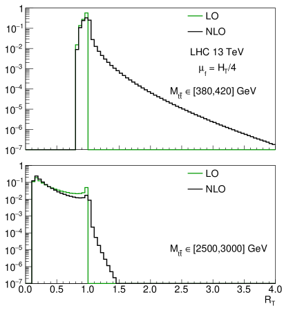
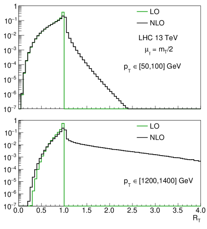
In figure 1, we show the distributions of $R_{T}$ in four kinematic regions, normalized to the integrated cross section in each region. The first is $M_{t\bar{t}}\in[380,420]$ GeV, representative of “low $M_{t\bar{t}}$”, $M_{t\bar{t}}\gtrsim 2m_{t}$; the second is $M_{t\bar{t}}\in[2500,3000]$ GeV, representative of “high $M_{t\bar{t}}$”, $M_{t\bar{t}}\gg 2m_{t}$; the third and fourth regions are $p_{T}\in[50,100]$ GeV and $p_{T}\in[1200,1400]$ GeV, representative of “low $p_{T}$” and “high $p_{T}$” respectively. We will also refer to these as “low-energy” and “high-energy” bins of $M_{t\bar{t}}$ or $p_{T}$. An interesting observation is that the differences between the LO and NLO distributions are quite distinctive in the four cases. It is the task of this subsection to explore the explanations and implications of these facts.

We first discuss the low-$M_{t\bar{t}}$ bin of the top-pair invariant mass distribution, whose $R_{T}$ distribution is shown in the top-left plot of figure 1. At both LO (the green curve) and NLO (the black curve), the distribution is peaked at $R_{T}\sim 1$, a fact following from eq. (54). However, at NLO, hard emissions generate a non-negligible fraction of the distribution in the $R_{T}>1$ region. In terms of a perturbative description beyond NLO, this indicates that while soft-gluon resummation can potentially improve the description in this bin, matching with NNLO in order to describe the $R_{T}>1$ region is needed for a precise prediction.

The $R_{T}$ distribution in the high-$M_{t\bar{t}}$ bin is displayed in the bottom-left plot of figure 1. A remarkable feature of this bin is that the $R_{T}$ distribution is peaked at values close to $R_{T}\sim 0.2$, both at LO and NLO. This feature can be traced to a property of the partonic cross section for $gg\to t\bar{t}$ scattering, namely that the Born diagrams possess $t$- and $u$-channel singularities in the limit $m_{t}\to 0$. These singularities are cut off by the finite value of the top-quark mass. However, we show below with analytic arguments that their presence implies that in the boosted regime where $m_{t}\ll M_{t\bar{t}}$ the integral over $\cos\theta$ used to calculate the differential cross section is dominated by the regions of small $R_{T}$. One implication of this feature is that the high-invariant mass region is especially amenable to soft-gluon resummation, as we shall see in section 5. Another is that, in spite of what one might expect, the most relevant perturbative scale in the high-energy tail of the top-pair invariant mass distribution is $H_{T}$ rather than $M_{t\bar{t}}$ itself. As a result, the partonic cross section, as well as the hard and soft functions appearing in the factorized form of the cross section in the soft limit, are better evaluated at scales $\mu\sim H_{T}$ in this region. This was indeed a main result of the fixed-order study of the top-pair invariant mass distribution to NNLO Czakon:2016dgf , which identified $\mu_{f}=H_{T}/4$ as the choice at which fixed-order perturbation theory converges best.

We now turn to the $R_{T}$ distributions in the two bins of top-quark $p_{T}$. The low and high $p_{T}$ regions are shown in the top-right plot and the bottom-right plot of figure 1, respectively. The Jacobian peaks at $R_{T}\sim 1$ are still present, similar to the $M_{t\bar{t}}$ case. The distributions exhibit long tails toward lower values of $R_{T}$. These come from the $t$- and $u$-channel singularities, the same effect at work in the high $M_{t\bar{t}}$ bin discussed in the last paragraph. On the other hand, the behavior of the NLO distribution in this case is rather different from the $M_{t\bar{t}}$ case. The measured value of the top quark $p_{T}$ can only constrain the combined $p_{T}$ of the anti-top-quark and the extra parton, but puts no constraints on their separate transverse momenta. It is therefore kinematically allowed to have the $t\bar{t}$ pair recoiled against a separate hard parton, such that one ends up with a large $H_{T}$ and a small $M_{t\bar{t}}$. This explains the long tail at the NLO towards $R_{T}>1$, particularly in the high $p_{T}$ bin. In fact, at $\mu_{f}=m_{T}/2$, one finds that $47$% of the distribution lies at $R_{T}>1$. From these facts, we expect that it is important to incorporate the effects of hard emissions for the $p_{T}$ distribution, especially in the high-$p_{T}$ region.

4.2 Scales for the $M_{t\bar{t}}$ distribution

The main goal of this and the next subsection is to identify the optimal choices of the hard scale $\mu_{h}$ and the soft scale $\mu_{s}$, based on the kinematic features of the hard and soft functions. Since the hard and soft functions may be evaluated analytically, this will also help to understand the kinematic features of the $R_{T}$ distribution given in the previous subsection.

The philosophy of RG-improved perturbation theory is to choose the matching scales such that the fixed-order expansion of the hard and soft functions is well behaved. The massless hard and soft functions depend on the kinematic invariants $M_{t\bar{t}}^{2}$, $t_{1}$ and $u_{1}$. As long as all of these scales are of the same size numerically, the choices $\mu_{h}\sim M_{t\bar{t}}$ and $\mu_{s}\sim M_{t\bar{t}}/\bar{N}$ free these functions of potentially large logarithmic corrections and thus ensure good perturbative convergence. The situation becomes more subtle in the boosted regime, where $m_{t}\ll M_{t\bar{t}}$. In that case, when the top quark is produced in the very forward region, $\cos\theta\to 1$, the kinematic invariants develop a hierarchy $|t_{1}|\ll M_{t\bar{t}}^{2}\sim|u_{1}|$. An analogous hierarchy develops for very backward production, with $|t_{1}|\leftrightarrow|u_{1}|$. Both of these situations correspond to the region $H_{T}\ll M_{t\bar{t}}$, since for Born kinematics

$$-t_{1}\big{|}_{m_{t}\to 0} \approx\frac{M_{t\bar{t}}^{2}}{2}(1-\cos\theta)+m_{t}^{2}\cos\theta\xrightarrow{\cos\theta\to 1}p_{T}^{2}+m_{t}^{2}\equiv m_{T}^{2}=H_{T}^{2}/4\,,$$ (55)

$$-u_{1}\big{|}_{m_{t}\to 0} \approx\frac{M_{t\bar{t}}^{2}}{2}(1+\cos\theta)-m_{t}^{2}\cos\theta\xrightarrow{\cos\theta\to-1}m_{T}^{2}=H_{T}^{2}/4\,.$$ (56)

On the other hand, the region where $m_{t}\sim M_{t\bar{t}}$ corresponds to $H_{T}\sim M_{t\bar{t}}$, irrespective of the value of $\cos\theta$.

The top-pair invariant mass distribution is calculated from the double differential cross section in eq. (11) by integrating over the scattering angle in the region $-1<\cos\theta<1$. At large $M_{t\bar{t}}$, the results for the $R_{T}$ distribution shown in the bottom-left panel of figure 1 and discussed in the previous subsection make clear that the integral is dominated by the region where $|\cos\theta|\sim 1$ and $R_{T}$ is significantly smaller than unity. This kinematic feature is explained by the fact that at Born level the $gg$ partonic cross section has $t$- and $u$-channel singularities, related to the hard function. For example, in the limit $t_{1}\to 0$, the LO hard function reads

$$\bm{H}_{gg}^{(0)}\big{|}_{t_{1}\to 0}=\frac{1}{2x_{t}}\begin{pmatrix}\frac{1}{N_{c}^{2}}&\frac{1}{N_{c}}&\frac{1}{N_{c}}\\ \frac{1}{N_{c}}&1&1\\ \frac{1}{N_{c}}&1&1\end{pmatrix}\,,$$ (57)

where $x_{t}\equiv-t_{1}/M_{t\bar{t}}^{2}$ and $N_{c}=3$ is the number of colors in QCD. The expression in the limit $u_{1}\to 0$ is obtained by replacing $x_{t}\to 1-x_{t}$. Therefore, at fixed $M_{t\bar{t}}\gg m_{t}$, the cross section gets large contributions from the region $H_{T}\ll M_{t\bar{t}}$, due to $t$- and $u$- channel enhancements in the $gg$ channel. The $q\bar{q}$ channel is free of such $t$- and $u$- channel enhancements.

The dynamical enhancement of the forward and backward scattering regions at large $M_{t\bar{t}}$ has important implications for the choice of the matching scales $\mu_{h}$ and $\mu_{s}$. We can study this issue analytically by expanding the higher-order corrections to the hard and soft functions in the limit $R_{T}\to 0$. The $gg$ partonic cross section is symmetric under the exchange of $t_{1}$ and $u_{1}$, so the $R_{T}\to 0$ limit can be easily obtained from the $x_{t}\to 0$ results, which we focus on for concreteness. While the soft function itself has no $1/x_{t}$ singularities in this limit, it enters the factorization formula in a matrix product with the hard function, so we must deal with both functions at once in order to take the correct limit of the differential cross section. This leads us to study the higher-order perturbative corrections at the level of the objects

$$\mathcal{H}^{\rm LO}_{ij}(\mu_{h}) =\alpha_{s}^{2}(\mu_{h})\,{\rm Tr}\left[\bm{H}_{ij}^{(0)}\widetilde{\bm{s}}_{ij}^{(0)}\right]\,,$$

$$\mathcal{H}^{\rm NLO}_{ij}(\mu_{h}) =\mathcal{H}^{\rm LO}_{ij}(\mu_{h})+\frac{\alpha_{s}^{3}(\mu_{h})}{4\pi}\,{\rm Tr}\left[\bm{H}_{ij}^{(1)}(\mu_{h})\widetilde{\bm{s}}_{ij}^{(0)}\right]\,,$$

$$\mathcal{H}^{\rm NNLO}_{ij}(\mu_{h}) =\mathcal{H}^{\rm NLO}_{ij}(\mu_{h})+\frac{\alpha_{s}^{4}(\mu_{h})}{(4\pi)^{2}}\,{\rm Tr}\left[\bm{H}_{ij}^{(2)}(\mu_{h})\widetilde{\bm{s}}_{ij}^{(0)}\right]\,,$$ (58)

and

$$\mathcal{S}^{\rm LO}_{ij} ={\rm Tr}\left[\bm{H}_{ij}^{(0)}\widetilde{\bm{s}}_{ij}^{(0)}\right]\,,$$

$$\mathcal{S}^{\rm NLO}_{ij}(\mu_{s}) =\mathcal{S}^{\rm LO}_{ij}+\frac{\alpha_{s}(\mu_{s})}{4\pi}{\rm Tr}\left[\bm{H}_{ij}^{(0)}\widetilde{\bm{s}}_{ij}^{(1)}(\mu_{s})\right]\,,$$

$$\mathcal{S}^{\rm NNLO}_{ij}(\mu_{s}) =\mathcal{S}^{\rm NLO}_{ij}(\mu_{s})+\left(\frac{\alpha_{s}(\mu_{s})}{4\pi}\right)^{2}{\rm Tr}\left[\bm{H}_{ij}^{(0)}\widetilde{\bm{s}}_{ij}^{(2)}(\mu_{s})\right]\,,$$ (59)

where we have suppressed the dependence of the matching functions on all parameters and scales other than $\mu_{h}$ and $\mu_{s}$. Explicit results for the NLO corrections can be written as

$$\frac{\mathcal{H}^{\rm NLO}_{gg}(\mu_{h})}{\mathcal{H}^{\rm LO}_{gg}(\mu_{h})}\bigg{|}_{t_{1}\to 0} =1\!+\!\frac{\alpha_{s}(\mu_{h})}{36\pi}\left[-78\ln^{2}\left(\frac{-t_{1}}{\mu_{h}^{2}}\right)\!+\!24\ln\left(\frac{-t_{1}}{\mu_{h}^{2}}\right)(3\!+\!2\ln x_{t})\!+\!37\pi^{2}-168\right]\,,$$

$$\frac{\mathcal{S}^{\rm NLO}_{gg}(\mu_{s})}{\mathcal{S}^{\rm LO}_{gg}}\bigg{|}_{t_{1}\to 0} =1\!+\!\frac{\alpha_{s}(\mu_{s})}{36\pi}\bigg{[}78\ln^{2}\left(\frac{-t_{1}}{\mu_{s}^{2}\bar{N}^{2}}\right)-48\ln\left(\frac{-t_{1}}{\mu_{s}^{2}\bar{N}^{2}}\right)\ln x_{t}+24\ln^{2}x_{t}\!+\!31\pi^{2}\bigg{]}\,,$$ (60)

and those for the NNLO corrections as

$$\frac{\mathcal{H}^{\text{NNLO}}_{gg}(\mu_{h})}{\mathcal{H}^{\text{NLO}}_{gg}(\mu_{h})}\bigg{|}_{t_{1}\to 0} =1\!+\!\left(\frac{\alpha_{s}(\mu_{h})}{4\pi}\right)^{2}\bigg{[}37.6\ln^{4}\left(\frac{-t_{1}}{\mu_{h}^{2}}\right)-\big{(}46.2\ln x_{t}+47.2\big{)}\ln^{3}\left(\frac{-t_{1}}{\mu_{h}^{2}}\right)$$

$$+\big{(}14.2\ln^{2}x_{t}+22.2\ln x_{t}-248\big{)}\ln^{2}\left(\frac{-t_{1}}{\mu_{h}^{2}}\right)$$

$$+\big{(}154\ln x_{t}+102\big{)}\ln\left(\frac{-t_{1}}{\mu_{h}^{2}}\right)+12.7\ln x_{t}+577\bigg{]}+\mathcal{O}(\alpha_{s}^{3})\,,$$

$$\frac{\mathcal{S}^{\text{NNLO}}_{gg}(\mu_{s})}{\mathcal{S}^{\text{NLO}}_{gg}}\bigg{|}_{t_{1}\to 0} =1\!+\!\left(\frac{\alpha_{s}(\mu_{s})}{4\pi}\right)^{2}\bigg{[}37.6\ln^{4}\left(\frac{-t_{1}}{\mu_{s}^{2}\bar{N}^{2}}\right)-\big{(}46.2\ln x_{t}+22.1\big{)}\ln^{3}\left(\frac{-t_{1}}{\mu_{s}^{2}\bar{N}^{2}}\right)$$

$$+\big{(}37.3\ln^{2}x_{t}+20.4\ln x_{t}+354\big{)}\ln^{2}\left(\frac{-t_{1}}{\mu_{s}^{2}\bar{N}^{2}}\right)$$

$$-\big{(}14.2\ln^{3}x_{t}+20.4\ln^{2}x_{t}+218\ln x_{t}+12.9\big{)}\ln\left(\frac{-t_{1}}{\mu_{s}^{2}\bar{N}^{2}}\right)$$

$$+3.56\ln^{4}x_{t}+6.81\ln^{3}x_{t}+109\ln^{2}x_{t}-42.6\ln x_{t}+356\bigg{]}+\mathcal{O}(\alpha_{s}^{3})\,,$$ (61)

where we have set $N_{c}=3$ and the number of light quarks to $N_{l}=5$ in the above equations.

An important feature of eqs. (60) and (61) is that both the NLO and the NNLO corrections depend on the two physical scales $-t_{1}$ and $M_{t\bar{t}}$ (through the ratio $x_{t}$). Therefore, any choice of $\mu_{h}$ and $\mu_{s}$ will lead to corrections of the form $\alpha_{s}^{n}\ln^{m}(x_{t})/x_{t}$ in the $x_{t}\to 0$ limit. However, the structure of such corrections is rather different for the hard and soft functions. For the hard function, the choice $\mu_{h}^{2}=-t_{1}$ frees the NLO corrections of such logarithmic corrections in $x_{t}\rightarrow 0$ limit, and reduces the logarithmic terms in the NNLO corrections to a single power of $\ln x_{t}$. On the other hand, the choice $\mu_{h}=M_{t\bar{t}}$ generates a double logarithmic series whose corrections have the form $\alpha_{s}^{n}\ln^{2n}(x_{t})/x_{t}$. Using that $\sqrt{-t_{1}}=H_{T}/2$ in the $x_{t}\to 0$ limit along with the symmetry of the $gg$ channel under $t_{1}\leftrightarrow u_{1}$, one thus expects the perturbative corrections from the hard function to the $M_{t\bar{t}}$ distribution to be well behaved across phase space with the choice $\mu_{h}=H_{T}/2$.

For the soft corrections $\mathcal{S}_{gg}$, double logarithmic corrections of the form $\alpha_{s}^{n}\ln^{2n}(x_{t})/x_{t}$ are generated even when $\mu_{s}=\sqrt{-t_{1}}/\bar{N}$ is chosen. To understand this result, we note that NLO corrections to the massless soft function can be written in the form Ferroglia:2012ku ; Ferroglia:2012uy

$$\widetilde{\bm{s}}^{(1)}=-\sum_{(I,J)=1}^{4}\bm{w}_{IJ}\left[\ln^{2}\left(\frac{s_{IJ}}{\mu_{s}^{2}\bar{N}^{2}}\right)+\frac{\pi^{2}}{6}+2{\rm Li}_{2}\left(1-\frac{s_{IJ}}{M_{t\bar{t}}^{2}}\right)\right]\,,$$ (62)

where $s_{12}=s_{34}=M_{t\bar{t}}^{2}$, $s_{13}=s_{24}=-t_{1}$, $s_{14}=s_{23}=-u_{1}$, and the sum over $(I,J)$ excludes the terms where $I=J$. The matrices ${\bm{w}}_{IJ}$ differ for the $q\bar{q}$ and $gg$ channels, and can be found in, for instance, Ferroglia:2012uy . The NLO corrections to the soft functions are thus characterized by the three different scales $s_{IJ}/\bar{N}$, the relative importance of each scale being determined by the properties of matrix elements ${\bm{w}}_{IJ}$, which are pure color factors. Taking the $x_{t}\to 0$ limit of $\mathcal{S}^{\rm(N)NLO}_{gg}$ then leads to the double logarithmic series mentioned above, irrespective of the choice of $\mu_{s}$.

The analytic results above give very useful insight into the nature of perturbative corrections arising from the hard and soft functions. In particular, they hint at the use of a $H_{T}$-based scale for the hard function, which is also a reasonable choice for the soft function. However, they are derived in the formal limit $R_{T}\to 0$, which for the top-pair invariant mass distribution is relevant because of a dynamical enhancement from $t$- and $u$- channel singularities in the high $M_{t\bar{t}}$ region. It is therefore useful and necessary to supplement these analytic arguments with a numerical study. To do this, we define NLO and NNLO $K$ factors for the hard and soft functions in the following way. For the hard functions, we evaluate the differential cross section with respect to $M_{t\bar{t}}$ using $\mathcal{H}^{\rm(N)NLO}_{ij}$ for the hard-scattering kernel in eq. (17), and define NLO and NNLO $K$ factors by dividing these results by those found using $\mathcal{H}^{\rm LO}_{ij}$. These ratios are indicated by $K_{ij}^{\rm H,(N)NLO}(M_{t\bar{t}},\mu_{h})$. The parton luminosity cancels in the ratio since the soft function is independent of the Mellin parameter $\bar{N}$ at LO, so we can write

$$K^{\rm H,NLO}_{ij}(M_{t\bar{t}},\mu_{h}) =\int_{-1}^{1}d\cos\theta\,\mathcal{H}^{\rm NLO}_{ij}(\mu_{h})\Bigg{/}\int_{-1}^{1}d\cos\theta\,\mathcal{H}^{\rm LO}_{ij}(\mu_{h})\,,$$

$$K^{\rm H,NNLO}_{ij}(M_{t\bar{t}},\mu_{h}) =\int_{-1}^{1}d\cos\theta\,\mathcal{H}^{\rm NNLO}_{ij}(\mu_{h})\Bigg{/}\int_{-1}^{1}d\cos\theta\,\mathcal{H}^{\rm LO}_{ij}(\mu_{h})\,.$$

Ratios $K^{\rm S,(N)NLO}(M_{t\bar{t}},\mu_{s})$, which take into account corrections from the soft function, are defined similarly. The important difference in the case of the soft function is that it depends on $\bar{N}$ and one must take the product with the Mellin-transformed parton luminosities before performing the inverse Mellin transform in order to get the contribution to the differential cross section. For simplicity, we use these luminosities evaluated at the scale $\mu_{f}=M_{t\bar{t}}$. We have checked that the luminosity dependence nearly completely cancels in the ratio defining the soft $K$ factors, so that the results depend very little on the exact choice of $\mu_{f}$ and also the collider energy.

Figure 2: The $K$ factors for the corrections to the hard (top) and soft (bottom) functions in the $gg$ channel as defined in the text, at $M_{t\bar{t}}=400$ GeV (left) and $M_{t\bar{t}}=2750$ GeV (right).

Numerical results for the hard and soft $K$ factors in the $gg$ channel are shown in figure 2, for two values of $M_{t\bar{t}}$. The first is $M_{t\bar{t}}=400$ GeV (left-hand plots), indicative of $m_{t}\sim M_{t\bar{t}}$, and the second is $M_{t\bar{t}}=2750$ GeV (right-hand plots), indicative of the high invariant-mass region where $m_{t}\ll M_{t\bar{t}}$. Results for the hard function, shown in the top two panels of the figure, are given for the two different parametric choices $\mu_{h}=rH_{T}$ (red lines) and $\mu_{h}=rM_{t\bar{t}}$ (blue lines), where $r$ is a numerical factor. Results for the soft function, shown in the bottom two panels of the figure, are given instead for $\mu_{s}=rH_{T}/\bar{N}$ (red lines) and $\mu_{s}=rM_{t\bar{t}}/\bar{N}$ (blue lines). At $M_{t\bar{t}}=400$ GeV there is little difference between the $K$ factors with the two different parametric choices, and both the hard and the soft $K$ factors are moderate as long as the proportionality factor $r$ is not too small. At the higher value of $M_{t\bar{t}}$, the corrections with the two different parametric scale choices differ by quite a large amount. For the hard function, the corrections remain moderate for $\mu_{h}\sim H_{T}/2$, as anticipated from the analysis above. For the soft function, the NLO corrections cannot be made smaller than about 50%. This happens, for instance, at $\mu_{s}\sim H_{T}/\bar{N}$. The $K$ factor at this scale is flat with respect to changes of $\mu_{s}$ around this value, at both the low and high values of $M_{t\bar{t}}$  and the NNLO corrections are also moderate.

The above analysis leads us to identify $\mu_{h}=H_{T}/2$ and $\mu_{s}=H_{T}/\bar{N}$ as a well-motivated choice of matching scales across the full range of $M_{t\bar{t}}$ in the $gg$ channel. We have checked that the soft and hard $K$ factors in the $q\bar{q}$ channel (which gives a considerably smaller contribution to the cross section at both large and small $M_{t\bar{t}}$) are also well behaved for these choices. Therefore, we will use these choices by default in all further numerical analysis of the $M_{t\bar{t}}$ distribution. Of course, at the level of differential cross sections the dependence on these scales cancels against that in the RG evolution factors, so that resummed results are independent of the exact choice at the order at which one is working. The unphysical, residual dependence can be reduced by calculating more orders in the logarithmic series, but with a proper choice of matching scales these higher-order terms are expected to be small corrections.

It is worth noting that Pecjak:2016nee , as well as all other works on soft-gluon resummation with PIM kinematics, used $M_{t\bar{t}}$-based matching scales instead of $H_{T}$-based ones. For moderate $M_{t\bar{t}}$ there is little difference, but at higher $M_{t\bar{t}}$ the perturbative uncertainties estimated from $\mu_{h}$ and $\mu_{s}$ variations are larger with the $M_{t\bar{t}}$-based choice. Some numerical results with $M_{t\bar{t}}$-based choices are given at the end in appendix A.

4.3 Scales for the $p_{T}$ distribution

Figure 3: The $K$ factors for the corrections to the hard (top) and soft (bottom) functions in the $gg$ channel as defined in the text, at $p_{T}=75$ GeV (left) and $p_{T}=1300$ GeV (right).

We now turn our attention to the top-quark $p_{T}$ distribution. We again motivate a suitable choice of $\mu_{h}$ and $\mu_{s}$ by studying $K$ factors for the hard and soft functions analogous to those for the $M_{t\bar{t}}$ distribution, but this time obtained by substituting the hard-scattering kernel in eq. (23) with the appropriate terms in eqs. (4.2) and (4.2) before inverting the Mellin transform to compute the cross section as a function of $p_{T}$. We show the results in figure 3 for a high and a low value of $p_{T}$, examining both $M_{t\bar{t}}$ and $m_{T}$ based scales. Note that while $K^{H,(N)NLO}(M_{t\bar{t}},\mu_{h})$ displayed explicitly in eq. (4.2) can be calculated without reference to the parton luminosities, this is not the case for $K^{H,(N)NLO}(p_{T},\mu_{h})$. We used $\mu_{f}=m_{T}$ in the luminosities in calculating both the hard and soft $K$ factors, and have checked that varying $\mu_{f}$ to other values produces only a small effect in the $K$ factor ratios.

The soft and hard $K$ factors exhibit only a mild hierarchy between the two types of scale choices in the low-$p_{T}$ region, which is even smaller in the high-$p_{T}$ region. This can be understood from figure 1, which shows that in both $p_{T}$ regions the cross section sits mainly at $2m_{T}\sim M_{t\bar{t}}$ due to the Jacobian peak at $R_{T}=1$. The $K$ factors are moderate when $\mu_{h}=m_{T}$ and $\mu_{s}=2m_{T}/\bar{N}$, and we shall use these as the default choices in our resummed calculations. Recall that in the soft limit the $p_{T}$ of the top is equal to that of the anti-top, so that $m_{T}=H_{T}/2$ and these are the exact same choices as for the $M_{t\bar{t}}$ distribution after a trivial renaming.

5 Results and discussion

In this section we give our main results for the top-pair invariant mass and (anti) top-quark $p_{T}$ distributions, as well as the total cross section, with a focus on comparing NNLO results with NNLO+NNLL^′ ones. Some further comparisons across different perturbative orders and between standard and threshold resummed PDFs are presented in appendices A and B respectively. Although we present only a limited set of results for the LHC operating at a center-of-mass energy of $\unit{13}{}$, distributions with alternate binning and at different collider energies can be produced on request from the authors.

Figure 4: Results for the absolute (left) and normalized (right) top-pair invariant mass distribution at the LHC with $\sqrt{s}=13$ TeV. In all cases the ratio is to the NNLO result with $\mu_{f}=H_{T}/4$. The uncertainty bands are obtained through scale variations as described at the beginning of section 5 and in eqs. (5) and (65).

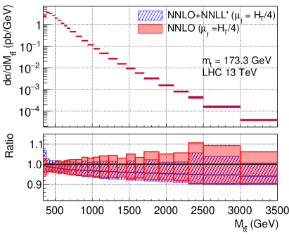
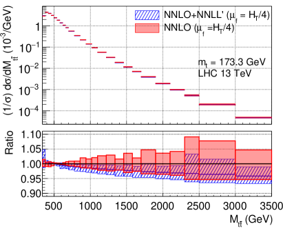
Results for the absolute (normalized) $M_{t\bar{t}}$ distribution are shown in left (right) panel of figure 4. The NNLO results use $\mu_{f}=H_{T}/4$ by default (we shall always set the renormalization scale appearing in the NNLO calculation to $\mu_{r}=\mu_{f}$ unless otherwise specified), which is the scale favored by the analysis of perturbative convergence of the fixed-order series performed in Czakon:2016dgf . The NNLO+NNLL^′ results are obtained from the matching relation eq. (5). All pieces of that equation must be evaluated at a common $\mu_{f}$, which is also chosen as $\mu_{f}=H_{T}/4$ by default. In addition, we draw on the analysis of the previous section and use $\mu_{h}=H_{T}/2$ and $\mu_{s}=H_{T}/\bar{N}$ by default, as well as $\mu_{dh}=m_{t}$ and $\mu_{ds}=m_{t}/\bar{N}$. In both the NNLO and the NNLO+NNLL^′ results, the bands in figure 4 represent perturbative uncertainties estimated through scale variations. For the NNLO calculation, we obtain the bands by keeping the factorization and renormalization scales equal and varying them up and down by a factor of two. For the NNLO+NNLL^′ calculation, both the factorization scales and the resummation scales are independently varied in the interval $\left[\mu_{i,0}/2,2\mu_{i,0}\right]$, where $i\in\{f,h,s,dh,ds\}$ and the subscript “$0$” denotes the default value of that scale as previously specified. To determine the upper and lower uncertainties $\Delta O^{+}$ and $\Delta O^{-}$ for the cross section $O$ in a given bin, one first evaluates

$$\Delta O_{i}^{+}=\text{max}\{O(\kappa_{i}=1/2,\kappa_{i}=1,\kappa_{i}=2)\}-\bar{O}\,,$$

$$\Delta O_{i}^{-}=\text{min}\{O(\kappa_{i}=1/2,\kappa_{i}=1,\kappa_{i}=2)\}-\bar{O}\,,$$ (64)

for each scale $i$, where $\kappa_{i}=\mu_{i}/\mu_{i,0}$ and $\bar{O}$ denotes the value of the cross section as given by eq. (5) in that bin using the default scale choices. For example, $O(\kappa_{f}=2)$ means each term in eq. (5) is evaluated at $\mu_{f}=2\mu_{f,0}$, with all other scales set to their default value. The upper (lower) uncertainty bands are then given by $\bar{O}+\Delta O^{+}$ ($\bar{O}-\Delta O^{-}$), where

$$\Delta O^{\pm}=\sqrt{\sum_{i}\left(\Delta O_{i}^{\pm}\right)^{2}}\,,$$ (65)

so that this method amounts to adding the uncertainties from independent scale variations in quadrature.

Figure 5: Results for the absolute (left) and normalized (right) top-pair invariant mass distribution at the LHC with $\sqrt{s}=13$ TeV as a ratio to the NNLO result evaluated using $\mu_{f}=H_{T}/4$. The uncertainty bands are obtained through scale variations as described at the beginning of section 5 and in eqs. (5) and (65).

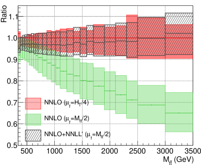
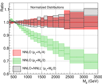
A remarkable feature of figure 4 is that the NNLO+NNLL^′ and NNLO results are in close agreement when $\mu_{f}=H_{T}/4$ is chosen. To add context to this result, we compare in figure 5 the ratio of the NNLO and NNLO+NNLL^′ results with $\mu_{f}=M_{t\bar{t}}/2$ to the NNLO result with $\mu_{f}=H_{T}/4$, using the same set of matching scales and method of estimating perturbative uncertainties as in figure 4. These two figures deliver a couple of important messages. Firstly, the NNLO+NNLL^′ result is rather stable against switching the factorization scale between $H_{T}$-based and $M_{t\bar{t}}$-based schemes. This implies that the even higher order corrections to the NNLO+NNLL^′ result are not so important. On the other hand, the NNLO result changes drastically when switching the schemes. In particular, higher order contributions beyond NNLO encoded in the resummation produce a very large effect for the choice $\mu_{f}=M_{t\bar{t}}/2$, as already forseen in Pecjak:2016nee . Given these observations, the close compatibility between the NNLO+NNLL^′ result (with either scale choice) and the NNLO result with $\mu_{f}=H_{T}/4$ is a highly non-trivial fact. This provides an important confirmation of the result of Czakon:2016dgf , which favors the choice $\mu_{f}=H_{T}/4$ for the fixed-order calculation of the $M_{t\bar{t}}$ distribution. The overall picture emerging from the above analysis is that the perturbative description of the top-quark pair invariant mass distribution is under good control.

Figure 6: Results for the absolute (left) and normalized (right) $p_{T,\text{avt}}$ distributions at the LHC with $\sqrt{s}=13$ TeV. In all cases the ratio is to the NNLO result with $\mu_{f}=m_{T}/2$. Uncertainty bands are obtained in complete analogy to those in figure 4.

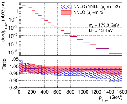
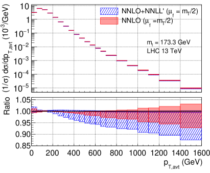
Results for the absolute (normalized) average top/anti-top ($p_{T,\text{avt}}$) distribution at NNLO and NNLO+NNLL^′ are shown in the left (right) panel of figure 6. The NNLO results (with which resummation is matched) have been calculated using the definition

$$\frac{d\sigma}{dp_{T,\text{avt}}}=\frac{1}{2}\left(\frac{d\sigma}{dp_{T,t}}+\frac{d\sigma}{dp_{T,\bar{t}}}\right)\,,$$ (66)

where $p_{T,t}$ ($p_{T,\bar{t}}$) denotes the transverse momentum of the top (anti-top) quark, and we have labeled the distributions in figure 6 accordingly. The $p_{T}$ distribution is calculated using the scale choice $\mu_{f}=m_{T}/2$ (where $m_{T}$ refers to the transverse mass of either the top or anti-top quark depending on the distribution under consideration), which is favored by the study Czakon:2016dgf . The resummed results use $\mu_{h}=m_{T}$ and $\mu_{s}=2m_{T}/\bar{N}$ by default, as justified in the previous section. The bands refer to perturbative uncertainties estimated through scale variations using the same procedure as for the $M_{t\bar{t}}$ distribution above. We see that the NNLO+NNLL^′ result is consistent with the NNLO one. On the other hand, we show in appendix A that upgrading matching with fixed-order from NLO+NNLL^′ to NNLO+NNLL^′ is an important effect for the $p_{T}$ distributions, especially in reducing the scale uncertainties in the high $p_{T}$ region. This is an important fact to keep in mind when using NLO-based Monte Carlo event generators to model $p_{T}$ distributions.

Figure 7: Predictions for the total top-pair production cross section at the LHC with $\sqrt{s}=13$ TeV, where the error bars represent perturbative uncertainty estimates through scale variations. The method for obtaining results and the uncertainty estimates at different values of $\mu_{f}$ is described in the second to last paragraph of section 5.

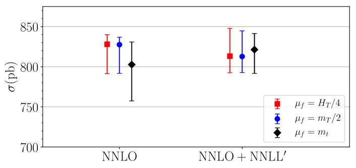
Finally, in figure 7 we show results for the total cross section, obtained in several different ways. The NNLO and NNLO+NNLL^′ results with $\mu_{f}=H_{T}/4$ are obtained by integrating the top-pair invariant mass distribution in figure 4, while those with $\mu_{f}=m_{T}/2$ are obtained by integrating the $p_{T}$ distribution in figure 6. In these results with dynamical scales, perturbative uncertainties are estimated through the same procedure of scale variations used for the distributions, and are displayed as error bars in figure 7. These are compared to the “standard” results for the total cross section, which are calculated using fixed scales with $\mu_{f}=\mu_{r}=m_{t}$ by default. We obtain them from the Top++ program Czakon:2011xx , which implements both the NNLO results from Czakon:2013goa as well as a soft-gluon resummation in the absolute threshold production limit $\beta_{t}\to 0$ Cacciari:2011hy . In these fixed scale results, perturbative uncertainties are estimated in both the NNLO and the NNLO+NNLL^′ results by varying $\mu_{f}$ and $\mu_{r}$ up and down by a factor of two using the seven-point method. Evidently, while this resummation result for the total cross section is also labelled NNLO+NNLL^′ in figure 7, one should keep in mind that it uses a different framework than the current work, including the treatment of resummation scales and how they are varied as just described.

From Figure 7 we see that the integral of both the NNLO+NNLL^′ $M_{t\bar{t}}$ distribution with $\mu_{f}=H_{T}/4$ and the NNLO+NNLL^′ $p_{T}$ distribution with $\mu_{f}=m_{T}/2$ yield nearly the same total cross section as the widely quoted result from the Top++ program. This shows that the results of this work not only provide the most precise QCD results for the top pair invariant mass distribution and the top quark transverse momentum distribution across phase space, but also give the correct normalization for these distributions.

6 Conclusions

In this paper we combined state-of-the-art results from soft-gluon resummation (NNLL^′) and fixed-order perturbation theory (NNLO) in order to produce NNLO+NNLL^′ predictions for the top-pair invariant mass and the average top/anti-top quark $p_{T,\text{avt}}$ distributions at hadron colliders. These results represent the most complete QCD calculations of these observables to date. They are also the first instance where an NNLO calculation has been supplemented with resummation in a process where the Born-level cross section contains four partons and thus has non-trivial matrix structure in color space.

The resummation formalism used here contains several elements which have not appeared in the literature so far. Some of these involve the details of weaving together three different kinds of calculations to obtain results optimized throughout phase space. In this procedure, it is crucial to avoid counting the same contribution more than once. In particular, in section 2 we presented a matching procedure which allows us to combine NNLO results in fixed order Czakon:2016dgf , NNLL${}_{b}^{\prime}$ results in a joint resummation of overlapping soft and collinear logarithms Ferroglia:2012ku , and NNLL_m results in pure soft-gluon resummation Ahrens:2010zv , in order to achieve what we have called NNLO+NNLL^′ accuracy. All ingredients required to implement this matching procedure, as well as the resummation itself, carried out in Mellin space, were given in section 3 and appendix C.

Our analysis in section 4 revealed some important kinematic features of the $M_{t\bar{t}}$ and $p_{T}$ distributions. These can not only be understood analytically using results from soft-gluon resummation, but also affect its implementation, and are useful to keep in mind when interpreting the numerical results for the $M_{t\bar{t}}$ and $p_{T}$ distributions given in section 5. In the case of the $M_{t\bar{t}}$ distribution, the analysis of section 4 demonstrates that in the boosted regime where $m_{t}\ll M_{t\bar{t}}$, the most relevant hard scale is not $M_{t\bar{t}}$ itself but rather $H_{T}$. This fact is related to the dynamical enhancement of the forward and backward scattering regions due to the $t$- and $u$-channel diagrams appearing in the Born level partonic cross section in the $gg$ initiated production process. We used this feature to identify a well-motivated set of matching scales for the kinematics-dependent hard and soft functions appearing in the resummation formalism, and also to argue that the high $M_{t\bar{t}}$ region is particularly amenable to soft gluon resummation. On the other hand, we observed that the high-energy region of the $p_{T}$ distribution is rather sensitive to hard emissions, so that matching resummation with NNLO is an essential improvement. This is certainly the case for the analytic resummation performed here, but should also be kept in mind when predicting the high-energy tail of the $p_{T}$ distribution with NLO-based event generators.

In section 5 we presented numerical results for the absolute and normalized $M_{t\bar{t}}$ and $p_{T,\text{avt}}$ distributions, as well as the total cross section, valid to NNLO+NNLL^′. For the $p_{T,\text{avt}}$ distribution the resummation effects are mild, especially at the scale $\mu_{f}=m_{T}/2$ favored by the NNLO analysis of perturbative convergence in Czakon:2016dgf . For the $M_{t\bar{t}}$ distribution, an interesting outcome of our analysis is the stability of the NNLO+NNLL^′ results under parametric changes in $\mu_{f}$, as shown in figures 4 and 5. Given the large shifts in the NNLO calculation under such $\mu_{f}$ changes, it is an important result that the NNLO+NNLL^′ results stabilize the differential cross section close to the NNLO prediction with $\mu_{f}=H_{T}/4$, which is the setting favored by Czakon:2016dgf and currently being used in all NNLO phenomenology. The consistency between the NNLO and NNLO+NNLL^′ results gives us confidence that even higher-order corrections are under good control.

Appendix A Perturbative stability across orders

Figure 8: Cross sections obtained for two sample bins, $M_{t\bar{t}}=[380-420]\,$ (upper plot) and $M_{t\bar{t}}=[2500-3000]\,$ (lower plot). The default value of $\mu_{f}$ is indicated explicitly, and the error bars represent perturbative uncertainties estimated through scale variations as described at the beginning of section 5 and in eqs. (5) and  (65).

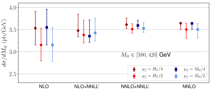
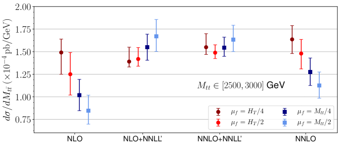
In this section we perform some comparisons of results for the top-pair invariant mass and average top/anti-top-quark $p_{T}$ distribution across different perturbative orders.

Figure 8 displays results for the cross section at (N)NLO and (N)NLO+NNLL^′ in the same low-energy and high-energy bins of $M_{t\bar{t}}$ considered in section 4.1. The NLO results are generated using NLO PDFs, while all other results are generated using NNLO PDFs (including the NLO+NNLL^′ ones). The resummed results use the default matching scales from section 5. The figure compares results obtained with the default $\mu_{f}$ indicated explicitly in the figure legend, with perturbative uncertainties estimated through scale variations and displayed as error bars. In both bins, adding resummation to the fixed-order result is a clear improvement: the (N)NLO+NNLL^′ results are considerably more stable against $\mu_{f}$ variations than the (N)NLO ones, especially in the high $M_{t\bar{t}}$ bin. An important message to be drawn from the figure is that the NNLO+NNLL^′ results at different $\mu_{f}$ congregate near the NNLO one with $\mu_{f}=H_{T}/4$.

Figure 9: Same as figure 8 but for the $p_{T,\text{avt}}$ distribution.

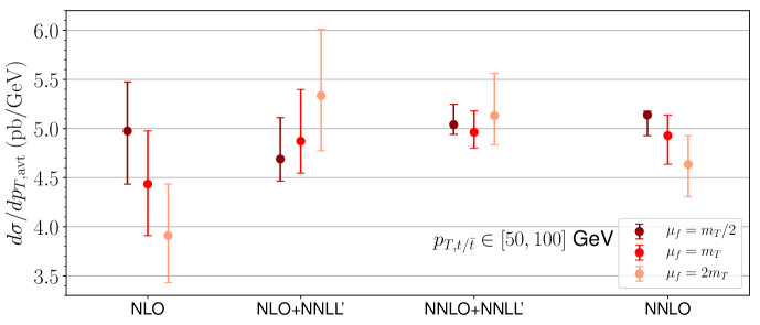
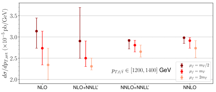
Figure 9 shows results for the $p_{T,\text{avt}}$ distribution at different perturbative orders in the two sample bins considered in section 4.1. The resummed results use the same default matching scales as in section 5 and are completely analogous to those in figure 8. Compared to the $M_{t\bar{t}}$ distribution, where the parametric difference between the $H_{T}$ and $M_{t\bar{t}}$-based $\mu_{f}$ is large, there is no such hierarchy of scales to consider for the $p_{T}$ distribution. Therefore, we have shown results for three different $m_{T}$-based choices, ranging from $\mu_{f}=m_{T}/2$ to $\mu_{f}=2m_{T}$ by default. While the resummation is of some benefit in stabilizing the (N)NLO results in the low-$p_{T}$ bin, the picture is less clear in the high-$p_{T}$ bin. For instance, there is a dramatic reduction in $\mu_{f}$ dependence in the NNLO+NNLL^′ results compared to the NLO+NNLL^′ ones. This is an indication that the high-$p_{T}$ region is more sensitive to hard radiation than the high-$M_{t\bar{t}}$ region. We have given some qualitative explanations for why this should be the case when discussing the $R_{T}$ distribution in section 4.1. Numerically, we have found that the NLO results for the high-$p_{T}$ region of the distribution are quite sensitive to both the $qg$ channel and the $R_{T}>1$ region, in a strongly $\mu_{f}$-dependent fashion. Soft-gluon resummation cannot stabilize such $\mu_{f}$ dependence, which explains the importance of matching to NNLO in fixed order.

	Bin (GeV)	NNLO+NNLL′ (pb)
$M_{t\bar{t}}$	$[380,420]$	$3.60$ ${}^{+4\%}_{-2\%}$${}^{+1\%}_{-1\%}$
	$[2500,3000]$	$(1.55\times 10^{-4})$ ${}^{+9\%}_{-4\%}$${}^{+3\%}_{-4\%}$
$p_{T,\text{avt}}$	$[50,100]$	$5.04$ ${}^{+4\%}_{-2\%}$${}^{+1\%}_{-1\%}$
	$[1200,1400]$	$(2.92\times 10^{-5})$ ${}^{+0\%}_{-7\%}$${}^{+1\%}_{-1\%}$

Table 2: Cross section in “high” and “low” energy bins. The first uncertainties refer to those from $\mu_{f}$ variation only while the second set are generated by the variation of the matching scales.

The uncertainties associated with each of the distributions presented here result from a combination of the uncertainties generated from the variation of each scale in accordance with eqs. (5) and (65). It is interesting to decompose the source of these uncertainty bands in terms of the contributions which arise from varying the factorization scale $\mu_{f}$ compared with the other matching scales. We present such a sample decomposition in table 2 for the two “low” and “high” energy bins used throughout section 4. We show the cross section in each bin with two sets of uncertainties, the first refers to those obtained through variations of $\mu_{f}$ alone while the second refers to the combined uncertainty generated by varying each of the matching scales. In most instances, the dominant contribution to the uncertainty arises from the variation of $\mu_{f}$. For the $M_{t\bar{t}}$ distribution at high $M_{t\bar{t}}$ the uncertainty from the matching scales is larger than at low $M_{t\bar{t}}$ while across the $p_{T}$ spectrum this source of uncertainty remains constant.

Figure 10: Comparison of the 3 results for the absolute (upper) and normalized (lower) $M_{t\bar{t}}$ distributions: 1) NLO+NNLL^′ with old scales (red bands); 2) NLO+NNLL^′ with new scales (blue bands on the left side); 3) NNLO+NNLL^′ with new scales (blue bands on the right side). They are all normalized by the central values of 1).

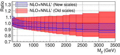
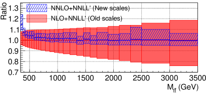
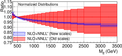
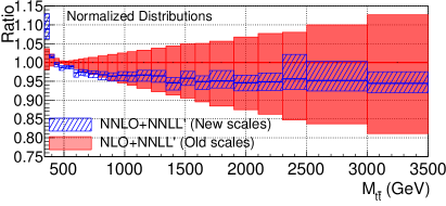
Finally, it is interesting to compare the results of the present work with the earlier resummation results at NLO+NNLL^′ accuracy in Pecjak:2016nee . To this end it is important to note that the differences between the current work and the work in Pecjak:2016nee are two-fold: 1) we have matched with the exact NNLO calculation here compared to an NLO matching in Pecjak:2016nee ; and 2) we have employed different settings of the factorization scale and the matching scales than Pecjak:2016nee . Concerning the scale choices, we remind the reader that in this work we by default use $\mu_{h}=H_{T}/2$, $\mu_{s}=H_{T}/\bar{N}$, $\mu_{f}=H_{T}/4$ for the $M_{t\bar{t}}$ distribution, and $\mu_{h}=m_{T}$, $\mu_{s}=2m_{T}/\bar{N}$, $\mu_{f}=m_{T}/2$ for the $p_{T}$ distribution. We refer to this scale setting as the “new scales”. On the other hand, Pecjak:2016nee by default uses $\mu_{h}=M_{t\bar{t}}$, $\mu_{s}=M_{t\bar{t}}/\bar{N}$, and $\mu_{f}=M_{t\bar{t}}/2$ (for the $M_{t\bar{t}}$ distribution) or $\mu_{f}=m_{T}$ (for the $p_{T}$ distribution). We call this scale setting the “old scales”.

In order to quantify the effect of switching to the new scales and the effect of matching with NNLO, we compare the 3 kinds differential cross sections: 1) NLO+NNLL^′ with old scales from Pecjak:2016nee ; 2) NLO+NNLL^′ with new scales from the present work; and 3) NNLO+NNLL^′ with new scales which are the best predictions of the present work. Such a comparison for the absolute as well as normalized $M_{t\bar{t}}$ distributions is shown in figure 10. It can be seen from the plots on the left side that, by changing to the new scales, the apparent scale uncertainties are reduced. This is a hint that with the new scale choice the higher order corrections are indeed smaller. The effect of matching with the NNLO results is shown in the plots on the right side of figure 10. We see that the matching changes the differential cross section most significantly in the low $M_{t\bar{t}}$ bins, which can be expected. A similar comparison in the case of $p_{T}$ distributions is shown in figure 11.

Figure 11: Same as figure 10 but for the $p_{T,\text{avt}}$ distribution.

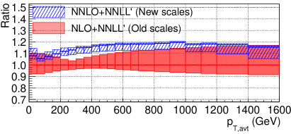
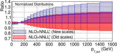
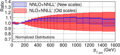
One can see that the change of default scales does not reduce the scale uncertainties (actually leading to larger uncertainties in the high $p_{T}$ bins). Matching with the NNLO is important here, which stabilizes the scale variation. Overall, the NNLO+NNLL^′ results are consistent with the NLO+NNLL^′ results when the new scales are used.

Appendix B Comparison with resummed PDFs

In the main part of this work, all computations have been carried out using the (N)NLO NNPDF3.0 PDF set Ball:2014uwa . However, one can also use threshold resummed PDFs Bonvini:2015ira , into which the effects of soft gluon radiation are incorporated. Including these contributions in the PDFs can produce non-negligible differences in threshold resummed cross section predictions when compared to those obtained with regular PDFs. An example of this can be found in Beenakker:2015rna , which considered sparticle pair production. In particular, for a large range of sparticle masses considered it was found that while $K$-factors (defined as the ratio of the resummed result to the fixed order one) obtained with regular PDFs were almost always greater than unity, this was not always the case when resummed PDFs were employed.

Although the resummed PDFs are obtained with a reduced data set and are therefore not yet suitable for precision calculations, we consider this an appropriate opportunity to explore their implications for top-quark pair production at the LHC. In order to compare results obtained with threshold resummed PDFs to those with standard PDFs we compute the $M_{t\bar{t}}$ and $p_{T,\text{avt}}$ distributions using the same settings as in section 5. To enable a fair comparison the NNPDF collaboration also provides PDFs which do not include threshold resummation but which are compiled from the same data set as the resummed ones. Specifically we use the NNPDF30_nnlo_disdytop PDFs as the benchmark for PDFs without threshold resummation and the NNPDF30_nnll_disdytop PDFs for those with threshold resummation.

Figure 12: Comparison of predictions obtained for the $M_{t\bar{t}}$ and $p_{T,\text{avt}}$ distributions with regular and resummed PDFs. Plotted are the NNLO prediction (red) using a fixed order PDF as well as the NNLO+NNLL^′ predictions computed both with fixed order (blue) and NNLL threshold resummed PDFs (purple). Each distribution is normalized to the NNLO one.

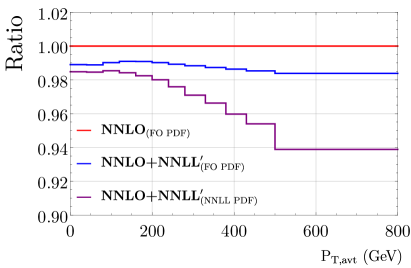
In figure 12 we compare the central values of the NNLO and NNLO+NNLL^′ predictions for the $p_{T,\text{avt}}$ and $M_{t\bar{t}}$ distributions, obtained using $\mu_{f}=m_{T}/2$ and and $\mu_{f}=H_{T}/4$, respectively. The NNLO predictions are calculated using the PDFs without resummation, while the NNLO+NNLL^′ predictions are computed using the PDFs with (labelled NNLL PDF) and without (labelled FO PDF) threshold resummation. In this manner, the NNLO and NNLO+NNLL^′ predictions with the fixed order PDFs act as an equivalent set of predictions to those in the main part of our paper, but now with a PDF set which can be compared to those incorporating threshold resummation. The left plot in figure 12 shows the $M_{t\bar{t}}$ distribution, where the effect of using resummed PDFs is significant. Here the use of resummed PDFs produces a suppression in the cross section at high $M_{t\bar{t}}$ compared to predictions produced with regular fixed order PDFs. The plot on the right, showing the $p_{T,\text{avt}}$ distribution, also displays noticeable changes. Here again the resummed PDFs produce a greater suppression of the cross section in the tail of the distribution than when regular PDFs are used. It will be interesting to perform further studies using resummed PDFs in the future as the fits improve and experimental measurements in the tails of these distributions become more accurate.

Appendix C The RG exponents

In this appendix we collect explicit expressions for the RG exponents appearing in eqs. (35), (3.3), and (3.3). In order to ease notation we introduce the following shorthand

$$L_{h}=\ln\frac{M_{t\bar{t}}^{2}}{\mu_{h}^{2}}\,,\quad L_{s}=\ln\frac{M_{t\bar{t}}^{2}}{\bar{N}^{2}\mu_{s}^{2}}\,,\quad L_{dh}=\ln\frac{m_{t}^{2}}{\mu_{dh}^{2}}\,,\quad L_{ds}=\ln\frac{m_{t}^{2}}{\bar{N}^{2}\mu_{ds}^{2}}\,,$$

and remind the reader that

$$\lambda_{i}=\frac{\alpha_{s}(\mu_{h})}{2\pi}\beta_{0}\ln\frac{\mu_{h}}{\mu_{i}}\,.$$

Perturbative expansions of the anomalous dimensions and beta function are given by

$$\gamma(\alpha_{s})= \left(\frac{\alpha_{s}}{4\pi}\right)\gamma_{0}+\left(\frac{\alpha_{s}}{4\pi}\right)^{2}\gamma_{1}+\left(\frac{\alpha_{s}}{4\pi}\right)^{3}\gamma_{2}+\ldots\,,$$

$$\beta(\alpha_{s})= -2\alpha_{s}\bigg{[}\left(\frac{\alpha_{s}}{4\pi}\right)\beta_{0}+\left(\frac{\alpha_{s}}{4\pi}\right)^{2}\beta_{1}+\ldots\bigg{]}\,.$$

Note that since the $g$-functions are derived from the part of the evolution functions in eqs. (29) and (3.3) which are proportional to the identity matrix in color space, the factors of $i\pi$ which appear there cancel out in the resummed cross section. As such, we do not retain these $i\pi$ factors in our expressions for the $g$-functions.

C.1 Soft limit

First, we present the $g^{m}_{i}$ functions appearing in the evolution factor eq. (35) for the threshold resummed result:

$$g^{m}_{1}(\lambda_{s},\lambda_{f}) =\frac{\Gamma_{0}}{2\beta_{0}^{2}}\Bigg{[}\lambda_{s}+(1-\lambda_{s})\ln(1-\lambda_{s})+\lambda_{s}\ln(1-\lambda_{f})\Bigg{]}\,,$$ (67)

$$g^{m}_{2}(\lambda_{s},\lambda_{f}) =\frac{\Gamma_{0}\beta_{1}}{2\beta_{0}^{3}}\Bigg{[}\ln(1-\lambda_{s})+\frac{1}{2}\ln^{2}(1-\lambda_{s})\Bigg{]}-\frac{\Gamma_{1}}{2\beta_{0}^{2}}\ln(1-\lambda_{s})+\frac{\gamma_{0}^{\phi}}{\beta_{0}}\ln\frac{1-\lambda_{s}}{1-\lambda_{f}}$$

$$+\frac{\Gamma_{0}}{2\beta_{0}}L_{s}\ln\frac{1-\lambda_{s}}{1-\lambda_{f}}+\frac{\Gamma_{0}}{2\beta_{0}}L_{h}\ln(1-\lambda_{f})$$

$$+\frac{1}{1-\lambda_{f}}\Bigg{\{}\frac{\Gamma_{0}\beta_{1}}{2\beta_{0}^{3}}\lambda_{s}\,[1+\ln(1-\lambda_{f})]-\frac{\Gamma_{1}}{2\beta_{0}^{2}}\lambda_{s}\Bigg{\}}\,,$$ (68)

$$g^{m}_{3}(\lambda_{s},\lambda_{f}) =\frac{1}{1-\lambda_{s}}\Bigg{\{}\frac{\Gamma_{0}\beta_{1}^{2}}{4\beta_{0}^{4}}\bigg{[}\lambda_{s}+2\lambda_{s}\ln(1-\lambda_{s})+\ln^{2}(1-\lambda_{s})\bigg{]}$$

$$\hskip 40.00006pt+\frac{\Gamma_{0}\beta_{2}}{2\beta_{0}^{3}}\bigg{[}\frac{\lambda_{s}}{2}+(1-\lambda_{s})\ln(1-\lambda_{s})\Bigg{]}-\frac{\Gamma_{1}\beta_{1}}{2\beta_{0}^{3}}\bigg{[}\frac{3}{2}\lambda_{s}+\ln(1-\lambda_{s})\bigg{]}$$

$$\hskip 40.00006pt+\frac{\Gamma_{2}}{4\beta_{0}^{2}}\lambda_{s}+\frac{\beta_{1}\gamma_{0}^{\phi}}{\beta_{0}^{2}}\big{[}1+\ln(1-\lambda_{s})\big{]}-\frac{\gamma_{1}^{\phi}}{\beta_{0}}$$

$$\hskip 40.00006pt+\frac{\Gamma_{0}\beta_{1}}{2\beta_{0}^{2}}\Big{[}\big{[}1+\ln(1-\lambda_{s})\big{]}L_{s}-(1-\lambda_{s})L_{h}\Big{]}\!+\!\frac{\Gamma_{1}}{2\beta_{0}}\big{[}(1-\lambda_{s})L_{h}-L_{s}\big{]}\Bigg{\}}$$

$$+\frac{1}{1-\lambda_{f}}\Bigg{\{}-\frac{\Gamma_{0}\beta_{1}^{2}}{2\beta_{0}^{4}}\lambda_{s}+\frac{\Gamma_{0}\beta_{2}}{2\beta_{0}^{3}}\lambda_{s}-\frac{\gamma_{0}^{\phi}\beta_{1}}{\beta_{0}^{2}}\big{[}1+\ln(1-\lambda_{f})\big{]}+\frac{\gamma_{1}^{\phi}}{\beta_{0}}$$

$$\hskip 40.00006pt+\frac{\Gamma_{1}}{2\beta_{0}}\big{[}L_{s}-L_{h}\big{]}+\frac{\Gamma_{0}\beta_{1}}{2\beta_{0}^{2}}\big{[}L_{h}-L_{s}\big{]}\big{[}1+\ln(1-\lambda_{f})\big{]}\Bigg{\}}$$

$$+\frac{\lambda_{s}}{(1-\lambda_{f})^{2}}\Bigg{\{}\!\frac{\Gamma_{0}\beta_{1}^{2}}{4\beta_{0}^{4}}\bigg{[}1-\ln^{2}(1-\lambda_{f})\bigg{]}-\!\frac{\Gamma_{0}\beta_{2}}{4\beta_{0}^{3}}\!+\!\frac{\Gamma_{1}\beta_{1}}{2\beta_{0}^{3}}\bigg{[}\frac{1}{2}\!+\!\ln(1-\lambda_{f})\bigg{]}-\frac{\Gamma_{2}}{4\beta_{0}^{2}}\!\Bigg{\}}\,.$$ (69)

C.2 Boosted-soft limit

Here we present the $g$-functions which appear in the evolution factors eqs. (3.3) and (3.3) for the boosted-soft resummation formula. The functions $g_{i}$ are simply given by their massive counterparts ($g_{i}^{m}$ as above) using the replacement,

$$\gamma^{\phi} \rightarrow\gamma^{\phi}+\gamma^{\phi_{q}}\,,$$

for each instance of $\gamma^{\phi}$ in the $g_{i}^{m}$ in appendix C.1. Each instance of $\Gamma_{\rm cusp}(\alpha_{s})$ in $g_{i}^{m}$ is replaced with $A(\alpha_{s})$ (this is due to the presence of $S_{A}$ and $a_{A}$ rather than $S_{\Gamma}$ and $a_{\Gamma}$ in eq. (3.3)) with $A(\alpha_{s})$ given by

$$A(\alpha_{s})\rightarrow\begin{dcases}2\Gamma_{\rm cusp}^{q},&q\bar{q}\text{-channel}\\ \Gamma_{\rm cusp}^{q}+\Gamma_{\rm cusp}^{g},&gg\text{-channel}\,.\end{dcases}$$

We decompose each of the $g_{i}^{D}$, which are functions of three arguments into two two-argument functions $g^{D}_{i,dh}$ and $g^{D}_{i,ds}$ as follows

$$g^{D}_{i}(\lambda_{dh},\lambda_{ds},\lambda_{f})=g^{D}_{i,dh}(\lambda_{dh},\lambda_{f})+g^{D}_{i,ds}(\lambda_{ds},\lambda_{f})\,.$$

Using this decomposition, we present below the functions as used in this work.

$$g^{D}_{1,dh}(\lambda_{dh},\lambda_{f}) =\frac{\Gamma_{0}}{2\beta_{0}^{2}}\Bigg{[}\ln(1-\lambda_{dh})+\lambda_{dh}\left[1-\ln\left(\frac{1-\lambda_{dh}}{1-\lambda_{f}}\right)\right]\Bigg{]}\,,$$ (70)

$$g^{D}_{1,ds}(\lambda_{ds},\lambda_{f}) =-\frac{\Gamma_{0}}{2\beta_{0}^{2}}\Bigg{[}\ln(1-\lambda_{ds})+\lambda_{ds}\left[1-\ln\left(\frac{1-\lambda_{ds}}{1-\lambda_{f}}\right)\right]\Bigg{]}\,,$$ (71)

$$g^{D}_{2,dh}(\lambda_{dh},\lambda_{f}) =\frac{\beta_{1}\Gamma_{0}}{2\beta_{0}^{3}}\Bigg{[}\left[1+\frac{1}{2}\ln(1-\lambda_{dh})\right]\ln(1-\lambda_{dh})\Bigg{]}-\frac{\Gamma_{1}}{2\beta_{0}^{2}}\ln(1-\lambda_{dh})$$

$$-\frac{\gamma_{0}^{S}}{\beta_{0}}\ln(1-\lambda_{dh})+\frac{\Gamma_{0}}{2\beta_{0}}L_{dh}\ln(1-\lambda_{dh})-\frac{\gamma_{0}^{\phi_{q}}}{\beta_{0}}\ln\left(\frac{1-\lambda_{dh}}{1-\lambda_{f}}\right)$$

$$+\frac{1}{1-\lambda_{f}}\Bigg{\{}\frac{\beta_{1}\Gamma_{0}}{2\beta_{0}^{3}}\lambda_{dh}\big{[}1+\ln(1-\lambda_{f})\big{]}-\frac{\Gamma_{1}}{2\beta_{0}^{2}}\lambda_{dh}\Bigg{\}}\,,$$ (72)

$$g^{D}_{2,ds}(\lambda_{ds},\lambda_{f}) =-\frac{\beta_{1}\Gamma_{0}}{2\beta_{0}^{3}}\Bigg{[}\left[1+\frac{1}{2}\ln(1-\lambda_{ds})\right]\ln(1-\lambda_{ds})\Bigg{]}+\frac{\Gamma_{1}}{2\beta_{0}^{2}}\ln(1-\lambda_{ds})$$

$$+\frac{\gamma_{0}^{S}}{\beta_{0}}\ln(1-\lambda_{ds})-\frac{\Gamma_{0}}{2\beta_{0}}L_{dh}\ln(1-\lambda_{ds})-\frac{\Gamma_{0}}{2\beta_{0}}\big{[}L_{ds}-L_{dh}\big{]}\ln\left(\frac{1-\lambda_{ds}}{1-\lambda_{f}}\right)$$

$$+\frac{1}{1-\lambda_{f}}\Bigg{\{}-\frac{\beta_{1}\Gamma_{0}}{2\beta_{0}^{3}}\lambda_{ds}\big{[}1+\ln(1-\lambda_{f})\big{]}+\frac{\Gamma_{1}}{2\beta_{0}^{2}}\lambda_{ds}\Bigg{\}}\,,$$ (73)

$$g^{D}_{3,dh}(\lambda_{dh},\lambda_{f}) =-\frac{\beta_{1}^{2}\ \Gamma_{0}}{2\beta_{0}^{4}}\ln(1-\lambda_{dh})+\frac{\beta_{2}\Gamma_{0}}{2\beta_{0}^{3}}\ln(1-\lambda_{dh})$$

$$+\frac{1}{1-\lambda_{dh}}\Bigg{\{}\frac{\beta_{1}^{2}\Gamma_{0}}{4\beta_{0}^{4}}\big{[}1+\ln(1-\lambda_{dh})\big{]}^{2}+\frac{\beta_{2}\Gamma_{0}}{4\beta_{0}^{3}}-\frac{\beta_{1}\Gamma_{1}}{2\beta_{0}^{3}}\bigg{[}\frac{3}{2}+\ln(1-\lambda_{dh})\bigg{]}$$

$$\hskip 40.00006pt+\frac{\Gamma_{2}}{4\beta_{0}^{2}}-\frac{\beta_{1}}{\beta_{0}^{2}}\big{(}\gamma_{0}^{\phi_{q}}+\gamma_{0}^{S}\big{)}\big{[}1+\ln(1-\lambda_{dh})\big{]}+\frac{1}{\beta_{0}}\big{(}\gamma_{1}^{\phi_{q}}+\gamma_{1}^{S}\big{)}$$

$$\hskip 40.00006pt+\frac{\beta_{1}\Gamma_{0}}{2\beta_{0}^{2}}\big{[}1+\ln(1-\lambda_{dh})\big{]}L_{dh}-\frac{\Gamma_{1}}{2\beta_{0}}L_{dh}\Bigg{\}}$$

$$+\frac{1}{1-\lambda_{f}}\Bigg{\{}-\frac{\beta_{1}^{2}\Gamma_{0}}{2\beta_{0}^{4}}\lambda_{dh}+\frac{\beta_{2}\Gamma_{0}}{2\beta_{0}^{3}}\lambda_{dh}+\frac{\beta_{1}}{2\beta_{0}^{2}}\gamma_{0}^{\phi_{q}}\big{[}1+\ln(1-\lambda_{f})\big{]}-\frac{\gamma_{1}^{\phi_{q}}}{2\beta_{0}}$$

$$\hskip 40.00006pt+\frac{\beta_{1}\Gamma_{0}}{4\beta_{0}^{2}}\big{[}L_{ds}-L_{dh}\big{]}\big{[}1+\ln(1-\lambda_{f})\big{]}-\frac{\Gamma_{1}}{4\beta_{0}}\big{[}L_{ds}-L_{dh}\big{]}\Bigg{\}}$$

$$+\frac{1}{(1-\lambda_{f})^{2}}\Bigg{\{}\frac{\beta_{1}^{2}\Gamma_{0}}{4\beta_{0}^{4}}\lambda_{dh}\big{[}1-\ln^{2}(1-\lambda_{f})\big{]}-\frac{\beta_{2}\Gamma_{0}}{4\beta_{0}^{3}}\lambda_{dh}$$

$$\hskip 40.00006pt+\frac{\beta_{1}\Gamma_{1}}{2\beta_{0}^{3}}\lambda_{dh}\bigg{[}\frac{1}{2}+\ln(1-\lambda_{f})\bigg{]}-\frac{\Gamma_{2}}{4\beta_{0}^{2}}\lambda_{dh}\Bigg{\}}\,,$$ (74)

$$g^{D}_{3,ds}(\lambda_{ds},\lambda_{f}) =\frac{\beta_{1}^{2}\ \Gamma_{0}}{2\beta_{0}^{4}}\ln(1-\lambda_{ds})-\frac{\beta_{2}\Gamma_{0}}{2\beta_{0}^{3}}\ln(1-\lambda_{ds})$$

$$+\frac{1}{1-\lambda_{ds}}\Bigg{\{}-\frac{\beta_{1}^{2}\Gamma_{0}}{4\beta_{0}^{4}}\big{[}1+\ln(1-\lambda_{ds})\big{]}^{2}-\frac{\beta_{2}\Gamma_{0}}{4\beta_{0}^{3}}+\frac{\beta_{1}\Gamma_{1}}{2\beta_{0}^{3}}\bigg{[}\frac{3}{2}+\ln(1-\lambda_{ds})\bigg{]}$$

$$\hskip 40.00006pt-\frac{\Gamma_{2}}{4\beta_{0}^{2}}+\frac{\beta_{1}}{\beta_{0}^{2}}\gamma_{0}^{S}\big{[}1+\ln(1-\lambda_{ds})\big{]}-\frac{\gamma_{1}^{S}}{\beta_{0}}$$

$$\hskip 40.00006pt-\frac{\beta_{1}\Gamma_{0}}{2\beta_{0}^{2}}\big{[}1+\ln(1-\lambda_{ds})\big{]}L_{ds}+\frac{\Gamma_{1}}{2\beta_{0}}L_{ds}\Bigg{\}}$$

$$+\frac{1}{1-\lambda_{f}}\Bigg{\{}\frac{\beta_{1}^{2}\Gamma_{0}}{2\beta_{0}^{4}}\lambda_{ds}-\frac{\beta_{2}\Gamma_{0}}{2\beta_{0}^{3}}\lambda_{ds}+\frac{\beta_{1}}{2\beta_{0}^{2}}\gamma_{0}^{\phi_{q}}\big{[}1+\ln(1-\lambda_{f})\big{]}-\frac{\gamma_{1}^{\phi_{q}}}{2\beta_{0}}$$

$$\hskip 40.00006pt+\frac{\beta_{1}\Gamma_{0}}{4\beta_{0}^{2}}\big{[}L_{ds}-L_{dh}\big{]}\big{[}1+\ln(1-\lambda_{f})\big{]}-\frac{\Gamma_{1}}{4\beta_{0}}\big{[}L_{ds}-L_{dh}\big{]}\Bigg{\}}$$

$$+\frac{1}{(1-\lambda_{f})^{2}}\Bigg{\{}-\frac{\beta_{1}^{2}\Gamma_{0}}{4\beta_{0}^{4}}\lambda_{ds}\big{[}1-\ln^{2}(1-\lambda_{f})\big{]}+\frac{\beta_{2}\Gamma_{0}}{4\beta_{0}^{3}}\lambda_{ds}$$

$$\hskip 40.00006pt-\frac{\beta_{1}\Gamma_{1}}{2\beta_{0}^{3}}\lambda_{ds}\bigg{[}\frac{1}{2}+\ln(1-\lambda_{f})\bigg{]}+\frac{\Gamma_{2}}{4\beta_{0}^{2}}\lambda_{ds}\Bigg{\}}\,.$$ (75)

References

- (1) M. Aaboud et al. [ATLAS Collaboration], arXiv:1801.02052 [hep-ex].
- (2) M. Czakon, D. Heymes, A. Mitov, D. Pagani, I. Tsinikos and M. Zaro, JHEP 1710 (2017) 186 [arXiv:1705.04105 [hep-ph]].
- (3) W. Beenakker, A. Denner, W. Hollik, R. Mertig, T. Sack and D. Wackeroth, Nucl. Phys. B 411 (1994) 343.
- (4) J. H. Kuhn, A. Scharf and P. Uwer, Eur. Phys. J. C 45 (2006) 139 [hep-ph/0508092].
- (5) W. Bernreuther, M. Fücker and Z. G. Si, Phys. Lett. B 633 (2006) 54 Erratum: [Phys. Lett. B 644 (2007) 386] [hep-ph/0508091].
- (6) J. H. Kuhn, A. Scharf and P. Uwer, Eur. Phys. J. C 51 (2007) 37 [hep-ph/0610335].
- (7) W. Bernreuther, M. Fuecker and Z. G. Si, Phys. Rev. D 74 (2006) 113005 [hep-ph/0610334].
- (8) W. Hollik and M. Kollar, Phys. Rev. D 77 (2008) 014008 [arXiv:0708.1697 [hep-ph]].
- (9) W. Bernreuther, M. Fücker and Z. G. Si, Phys. Rev. D 78 (2008) 017503 [arXiv:0804.1237 [hep-ph]].
- (10) W. Bernreuther and Z. G. Si, Nucl. Phys. B 837 (2010) 90 [arXiv:1003.3926 [hep-ph]].
- (11) A. Denner, S. Dittmaier, S. Kallweit and S. Pozzorini, Phys. Rev. Lett. 106 (2011) 052001 [arXiv:1012.3975 [hep-ph]].
- (12) G. Bevilacqua, M. Czakon, A. van Hameren, C. G. Papadopoulos and M. Worek, JHEP 1102 (2011) 083 [arXiv:1012.4230 [hep-ph]].
- (13) W. Hollik and D. Pagani, Phys. Rev. D 84 (2011) 093003 [arXiv:1107.2606 [hep-ph]].
- (14) J. H. Kuhn and G. Rodrigo, JHEP 1201 (2012) 063 [arXiv:1109.6830 [hep-ph]].
- (15) A. V. Manohar and M. Trott, Phys. Lett. B 711 (2012) 313 [arXiv:1201.3926 [hep-ph]].
- (16) W. Bernreuther and Z. G. Si, Phys. Rev. D 86 (2012) 034026 [arXiv:1205.6580 [hep-ph]].
- (17) A. Denner, S. Dittmaier, S. Kallweit and S. Pozzorini, JHEP 1210 (2012) 110 [arXiv:1207.5018 [hep-ph]].
- (18) R. Frederix, Phys. Rev. Lett. 112 (2014) no.8, 082002 [arXiv:1311.4893 [hep-ph]].
- (19) J. H. Kühn, A. Scharf and P. Uwer, Phys. Rev. D 91 (2015) no.1, 014020 [arXiv:1305.5773 [hep-ph]].
- (20) J. M. Campbell, D. Wackeroth and J. Zhou, Phys. Rev. D 94 (2016) no.9, 093009 [arXiv:1608.03356 [hep-ph]].
- (21) D. Pagani, I. Tsinikos and M. Zaro, Eur. Phys. J. C 76 (2016) no.9, 479 [arXiv:1606.01915 [hep-ph]].
- (22) A. Denner and M. Pellen, JHEP 1608 (2016) 155 [arXiv:1607.05571 [hep-ph]].
- (23) M. Czakon, D. Heymes and A. Mitov, Phys. Rev. Lett. 116 (2016) no.8, 082003 [arXiv:1511.00549 [hep-ph]].
- (24) M. Czakon, D. Heymes and A. Mitov, JHEP 1704 (2017) 071 [arXiv:1606.03350 [hep-ph]].
- (25) P. Bärnreuther, M. Czakon and A. Mitov, Phys. Rev. Lett. 109 (2012) 132001 [arXiv:1204.5201 [hep-ph]].
- (26) M. Czakon and A. Mitov, JHEP 1212 (2012) 054 [arXiv:1207.0236 [hep-ph]].
- (27) M. Czakon and A. Mitov, JHEP 1301 (2013) 080 [arXiv:1210.6832 [hep-ph]].
- (28) M. Czakon, P. Fiedler and A. Mitov, Phys. Rev. Lett. 110 (2013) 252004 [arXiv:1303.6254 [hep-ph]].
- (29) M. Czakon, P. Fiedler and A. Mitov, Phys. Rev. Lett. 115 (2015) no.5, 052001 [arXiv:1411.3007 [hep-ph]].
- (30) A. Ferroglia, B. D. Pecjak and L. L. Yang, Phys. Rev. D 86 (2012) 034010 [arXiv:1205.3662 [hep-ph]].
- (31) B. D. Pecjak, D. J. Scott, X. Wang and L. L. Yang, Phys. Rev. Lett. 116 (2016) no.20, 202001 [arXiv:1601.07020 [hep-ph]].
- (32) V. Ahrens, A. Ferroglia, M. Neubert, B. D. Pecjak and L. L. Yang, JHEP 1009 (2010) 097 [arXiv:1003.5827 [hep-ph]].
- (33) R. Bonciani, S. Catani, M. L. Mangano and P. Nason, Nucl. Phys. B 529 (1998) 424 Erratum: [Nucl. Phys. B 803 (2008) 234] [hep-ph/9801375].
- (34) M. Czakon, A. Mitov and G. F. Sterman, Phys. Rev. D 80 (2009) 074017 [arXiv:0907.1790 [hep-ph]].
- (35) M. Beneke, P. Falgari, S. Klein and C. Schwinn, Nucl. Phys. B 855 (2012) 695 [arXiv:1109.1536 [hep-ph]].
- (36) M. Beneke, P. Falgari and C. Schwinn, Nucl. Phys. B 842 (2011) 414 [arXiv:1007.5414 [hep-ph]].
- (37) A. Ferroglia, S. Marzani, B. D. Pecjak and L. L. Yang, JHEP 1401 (2014) 028 [arXiv:1310.3836 [hep-ph]].
- (38) N. Kidonakis and G. F. Sterman, Nucl. Phys. B 505 (1997) 321 [hep-ph/9705234].
- (39) T. Becher, A. Broggio and A. Ferroglia, Lect. Notes Phys. 896 (2015) pp.1 [arXiv:1410.1892 [hep-ph]].
- (40) V. Ahrens, A. Ferroglia, M. Neubert, B. D. Pecjak and L. L. Yang, JHEP 1109 (2011) 070 [arXiv:1103.0550 [hep-ph]].
- (41) A. Broggio, A. Ferroglia, G. Ossola and B. D. Pecjak, JHEP 1609 (2016) 089 [arXiv:1607.05303 [hep-ph]].
- (42) A. Broggio, A. Ferroglia, B. D. Pecjak and L. L. Yang, JHEP 1702 (2017) 126 [arXiv:1611.00049 [hep-ph]].
- (43) A. Broggio, A. Ferroglia, G. Ossola, B. D. Pecjak and R. D. Sameshima, JHEP 1704 (2017) 105 [arXiv:1702.00800 [hep-ph]].
- (44) S. Moch, J. A. M. Vermaseren and A. Vogt, Nucl. Phys. B 726 (2005) 317 [hep-ph/0506288].
- (45) A. J. Buras, M. Jamin, M. E. Lautenbacher and P. H. Weisz, Nucl. Phys. B 370 (1992) 69 Addendum: [Nucl. Phys. B 375 (1992) 501].
- (46) M. Bonvini, S. Forte, M. Ghezzi and G. Ridolfi, Nucl. Phys. B 861 (2012) 337 [arXiv:1201.6364 [hep-ph]].
- (47) M. Bonvini, S. Forte, G. Ridolfi and L. Rottoli, JHEP 1501 (2015) 046 [arXiv:1409.0864 [hep-ph]].
- (48) A. Broggio, A. Ferroglia, B. D. Pecjak and Z. Zhang, JHEP 1412 (2014) 005 [arXiv:1409.5294 [hep-ph]].
- (49) A. Ferroglia, B. D. Pecjak, L. L. Yang, B. D. Pecjak and L. L. Yang, JHEP 1210 (2012) 180 [arXiv:1207.4798 [hep-ph]].
- (50) K. Melnikov and A. Mitov, Phys. Rev. D 70 (2004) 034027 [hep-ph/0404143].
- (51) J. G. Korner, Z. Merebashvili and M. Rogal, Phys. Rev. D 77 (2008) 094011 Erratum: [Phys. Rev. D 85 (2012) 119904] [arXiv:0802.0106 [hep-ph]].
- (52) B. Kniehl, Z. Merebashvili, J. G. Korner and M. Rogal, Phys. Rev. D 78 (2008) 094013 [arXiv:0809.3980 [hep-ph]].
- (53) M. Czakon, A. Mitov and S. Moch, Phys. Lett. B 651 (2007) 147 [arXiv:0705.1975 [hep-ph]].
- (54) M. Czakon, A. Mitov and S. Moch, Nucl. Phys. B 798 (2008) 210 [arXiv:0707.4139 [hep-ph]].
- (55) M. Bonvini and S. Marzani, JHEP 1409 (2014) 007 [arXiv:1405.3654 [hep-ph]].
- (56) S. Moch, J. A. M. Vermaseren and A. Vogt, Nucl. Phys. B 688 (2004) 101 [hep-ph/0403192].
- (57) T. Becher and M. Neubert, Phys. Rev. D 79 (2009) 125004 Erratum: [Phys. Rev. D 80 (2009) 109901] [arXiv:0904.1021 [hep-ph]].
- (58) T. Becher and M. Neubert, JHEP 0906 (2009) 081 Erratum: [JHEP 1311 (2013) 024] [arXiv:0903.1126 [hep-ph]].
- (59) A. Ferroglia, M. Neubert, B. D. Pecjak and L. L. Yang, Phys. Rev. Lett. 103 (2009) 201601 [arXiv:0907.4791 [hep-ph]].
- (60) A. Ferroglia, M. Neubert, B. D. Pecjak and L. L. Yang, JHEP 0911 (2009) 062 [arXiv:0908.3676 [hep-ph]].
- (61) N. Kidonakis, Phys. Rev. Lett. 102 (2009) 232003 [arXiv:0903.2561 [hep-ph]].
- (62) G. P. Korchemsky and A. V. Radyushkin, Nucl. Phys. B 283 (1987) 342.
- (63) G. P. Korchemsky and A. V. Radyushkin, Phys. Lett. B 279 (1992) 359 [hep-ph/9203222].
- (64) G. Wang, X. Xu, L. L. Yang, H. X. Zhu, in preparation.
- (65) P. Bärnreuther, M. Czakon and P. Fiedler, JHEP 1402 (2014) 078 [arXiv:1312.6279 [hep-ph]].
- (66) A. Kulesza, G. F. Sterman and W. Vogelsang, Phys. Rev. D 66 (2002) 014011 [hep-ph/0202251].
- (67) A. Buckley, J. Ferrando, S. Lloyd, K. Nordström, B. Page, M. Rüfenacht, M. Schönherr and G. Watt, Eur. Phys. J. C 75 (2015) 132 [arXiv:1412.7420 [hep-ph]].
- (68) M. Bonvini, arXiv:1212.0480 [hep-ph].
- (69) S. Catani, M. L. Mangano, P. Nason and L. Trentadue, Nucl. Phys. B 478 (1996) 273 [hep-ph/9604351].
- (70) S. Forte, G. Ridolfi, J. Rojo and M. Ubiali, Phys. Lett. B 635 (2006) 313 [hep-ph/0601048].
- (71) R. D. Ball et al. [NNPDF Collaboration], JHEP 1504 (2015) 040 [arXiv:1410.8849 [hep-ph]].
- (72) M. Bonvini et al., JHEP 1509 (2015) 191 [arXiv:1507.01006 [hep-ph]].
- (73) T. Hahn, Comput. Phys. Commun. 168 (2005) 78 [hep-ph/0404043].
- (74) M. Czakon and A. Mitov, Comput. Phys. Commun. 185 (2014) 2930 [arXiv:1112.5675 [hep-ph]].
- (75) M. Cacciari, M. Czakon, M. Mangano, A. Mitov and P. Nason, Phys. Lett. B 710 (2012) 612 [arXiv:1111.5869 [hep-ph]].
- (76) W. Beenakker, C. Borschensky, M. Krämer, A. Kulesza, E. Laenen, S. Marzani and J. Rojo, Eur. Phys. J. C 76 (2016) no.2, 53 [arXiv:1510.00375 [hep-ph]].