Fog Massive MIMO: A User-Centric Seamless Hot-Spot Architecture

Abstract

The decoupling of data and control planes, as proposed for 5G networks, will enable the efficient implementation of multitier networks where user equipment (UE) nodes obtain coverage and connectivity through the top-tier macro-cells, and, at the same time, achieve high-throughput low-latency communication through lower tiers in the hierarchy. This paper considers a new architecture for such lower tiers, dubbed fog massive MIMO, where the UEs are able to establish high-throughput low-latency data links in a seamless and opportunistic manner, as they travel through a dense “fog” of high-capacity wireless infrastructure nodes, referred to as remote radio heads (RRHs). Traditional handover mechanisms in dense multicell networks inherently give rise to frequent handovers and pilot sequence re-assignments, incurring, as a result, excessive protocol overhead and significant latency. In the proposed fog massive MIMO architecture, UEs seamlessly and implicitly associate themselves to the most convenient RRHs in a completely autonomous manner. Each UE makes use of a unique uplink pilot sequence, and pilot contamination is mitigated by a novel coded “on-the-fly” pilot contamination control mechanism. We analyze the spectral efficiency and the outage probability of the proposed architecture via stochastic geometry, using some recent results on unique coverage in Boolean models, and provide a detailed comparison with respect to an idealized baseline massive MIMO cellular system, that neglects protocol overhead and latency due to explicit user-cell association. Our analysis, supported by extensive system simulation, reveals that there exists a “sweet spot” of the per-pilot user load (number of users per pilot), such that the proposed system achieves spectral efficiency close to that of an ideal cellular system with the minimum distance user-base station association and no pilot/handover overhead.

I Introduction

5G technologies are expected to bring about great improvements with respect to a multitude of metrics, including user and cell throughput, end-to-end latency and massive device connectivity. They are also viewed as essential elements for enabling the much broader gamut of services envisioned, such as immersive applications (e.g., virtual/augmented/mixed reality) [1, 2], haptics [3], V2X (vehicle-to-everything) [4], and the Internet of Things [5]. To meet such ambitious and broad range of goals, operators would have to rely on a combination of additional resources, which include newly available licensed and unlicensed bands, network densification, large antenna arrays, and new PHY/network layer technologies. In particular, the wide range of performance objectives for such a disparate variety of services is not suited to the conventional “one-size fits all” approach of conventional single-tier cellular networks. For this reason, a key feature of 5G networks consists of the decoupling of data and control planes [6], in order to enable multi-tier networks [7]. In such architectures, user equipment (UE) nodes shall maintain coverage and connectivity through macro-cells operating at conventional frequency bands (1 to 3.5 GHz), with low propagation pathloss and good indoor penetration. While this tier stays at the top of the hierarchy and takes care of fundamental functionalities such as mobility management and general bookkeeping of the users in the system, high-throughput and low-latency data communication is supported by lower tiers in the hierarchy, formed by smaller and simpler infrastructure nodes operating at higher frequency bands with smaller range [8]. By means of a large number of remote radio heads (RRHs), deployed as a second tier, localized network densification can be used for hot-spot formation, in order to tackle the spatial non-uniformity in data traffic demands, which is one of the biggest challenges faced by wireless operators.

Massive MIMO suppresses the small-scale fading effects through channel hardening [10], resulting in an almost-deterministic wireless channel between the transmitter and receiver, which in turn simplifies rate and power allocation and yields superior spectral and energy efficiency. While massive MIMO has been mainly regarded as a technology for large and costly cellular base stations (BSs), the current technology trend considers higher and higher carrier frequencies and mass production for dense deployment, with corresponding decreasing size and costs. It is therefore expected that, in the near future, it will be possible to implement small and inexpensive RRHs with up to $\sim$100 antennas, each of which serving on average a relatively small number of users (e.g., $\sim$10) on same channel subband. Considering the fact that the main deployment cost for operators is represented by the number of sites (not number of antennas per site), to make the most out of BS sites, we focus on RRH with large antenna arrays, unlike single antenna site work such as [11].

Higher-frequency operation inherently implies shorter range, higher penetration loss, and shorter coherence time. Higher-frequency tiers would need to be denser. As a result, planned operation of such tiers becomes excessively costly and inefficient. Indeed, in a conventional small-cell architecture, the cell size is simply scaled down, while maintaining all functionalities in each small-cell BS. The performance of dense small-cell systems is therefore severely limited by several issues resulting from cell-size scale down, e.g., reduced cell isolation, excessive handoffs, asymmetric forward and reverse links, dynamic interference, and backhaul management [12]. Particularly, in the presence of high mobility (as for V2X applications), frequent handovers and per-cell pilot sequence re-assignment may incur a large protocol overhead and significant latency. For example, when a finite number of mutually orthogonal pilot sequences are distributed among the users and are not re-allocated dynamically, it is unavoidable that the same pilot may be assigned to several users that may be in spatial proximity at some point in time (due to mobility). In this case, a dense massive MIMO deployment may incur severe multiuser interference due to pilot contamination [13].

I-A Contributions

This paper considers a new architecture for dense massive MIMO, dubbed fog massive MIMO, where the UEs are able to establish high-throughput and low-latency data links in a seamless and opportunistic manner, as they move through a dense “fog” of high-capacity multiantenna RRHs. Our architecture follows a user-centric approach (see also our preliminary work in [14, 15]). In particular, fog massive MIMO realizes the advantages of distributed antenna systems such as cell-free operations and efficient interference management, while preserving the simplicity of localized (i.e., per-RRH) physical layer processing. This is achieved by exploiting the channel state information obtained via time-division duplexing (TDD) uplink (UL) downlink (DL) reciprocity, in conjunction with two mechanisms: (i) On-the-fly pilot contamination control at the physical layer; (ii) Geographic routing with packet replication at the network layer.

The proposed on-the-fly pilot contamination control mechanism allows each RRH to decide autonomously and instantaneously whether a received UL pilot is free from contamination. Only the packets of the UEs corresponding to uncontaminated pilots are decoded in the UL slot and subsequently served via multiuser MIMO precoding in the DL slot.

Geographic routing with packet replication allows any user, with high probability, to be in the proximity of a sufficiently large number of RRHs with data packets ready to send, thus creating opportunistic macro-diversity opportunities. Hence, it is not really important “from which RRH” a given UE receives a requested packet, as long as there exists some RRHs nearby that can provide such packet.

Fig. 1 shows the concept of the proposed fog massive MIMO system. In Fig. 1, three UEs making use of orthogonal UL pilots receive their requested DL packet from some surrounding RRHs, which beamform the packet such that the signal combine coherently, achieving a macro-diversity effect. In Fig. 1 we illustrate the idea of on-the-fly pilot contamination control. In this case, the three UEs use the same UL pilot. Hence, some RRHs in the intersection of their transmission range suffer from contamination. These RRHs refrain from using this pilot for channel estimation and beamforming. Nevertheless, the UEs can still be served by other RRHs.

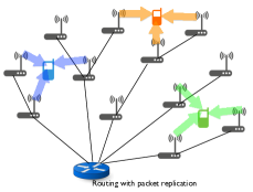
(a)

(b)

Figure 1: A fog massive MIMO network serving three UEs. In example (a), the UEs use orthogonal UL pilots, and receive their requested packet from possibly multiple RRHs (macro-diversity). Example (b) shows three UEs associated to the same UL pilot. The RRHs in the transmission range intersection regions detect pilot contamination and discard the corresponding channel estimate.

This altogether motivates the analysis of a fog massive MIMO system that we present here, with the following novel contributions:

1) We propose a simple coded UL pilot scheme that detects with arbitrarily high reliability (in the limit of large antennas) the pilot contamination through a very simple pilot matched filtering and threshold operation. This allows on-the-fly pilot contamination control on a per-slot basis, i.e., with minimal latency.

2) We leverage some recent results on unique coverage in Boolean models [16] to provide the performance analysis of the proposed fog massive MIMO system when the locations of UEs and RRHs are modeled via two independent Poisson point processes (PPPs). Our analysis yields the spatially averaged user spectral efficiency (b/s/Hz per user) and area spectral efficiency (b/s/Hz per unit area) through easy to compute integral approximation, extensively validated by Monte Carlo system simulation.

3) As a term of comparison, we consider an ideal cellular massive MIMO system with minimum distance UE-BS association and fractional pilot reuse (each cell uses a randomly selected subset of pilots from a pool of orthogonal UL pilots). For this system, we derive the expressions for the spatially averaged user and area spectral efficiencies in integral forms.

As expected, the ideal cellular system yields generally better performance than the (overhead-less) fog system, since it associates UEs to BSs according to the minimum distance and assumes an ideal intra-cell pilot management policy that guarantees mutually orthogonal pilots in each cell. In our comparison, we do not take into account the cost incurred by pilot allocation/reallocation at each handover in the presence of mobility, when users migrate from cell to cell. Instead of trying to quantify such overhead, which would be beyond the scope of this paper, we compare the ideal baseline cellular system with the fully practical proposed fog massive MIMO system, and identify the regime where the latter yields comparable performance with respect to its cellular counterpart.

I-B Relation to Cell-Free Massive MIMO

A system consisting of RRHs with local processing, geographic routing with packet replication, and somehow user-centric operations was recently proposed in [11] under the name of cell-free massive MIMO. This system makes use of a very large number of single-antenna RRHs. The key idea of cell-free massive MIMO is that in the DL, maximal-ratio transmission can be obtained by local combining of the user data packets with the complex conjugate of the channel coefficients at each RRH, without the need for centralized processing as in cloud radio access network (CRAN) architectures (e.g., see [17]). As in our scheme, the channel coefficients can be learned at each RRH via TDD reciprocity from UL pilots. Despite some similarities, cell-free massive MIMO and the fog massive MIMO proposed and analyzed in this paper are indeed quite different. First, in cell-free massive MIMO it is assumed that each RRH has full information on the channel large-scale gains from itself to all users in the system. Otherwise, for $K$ UEs with $Q$ orthogonal pilots, with $K>Q$, it is impossible for a RRH to associate a packet to the channel estimate produced from a given pilot observation, since the same pilot is associated to multiple users. As an alternative, cell-free massive MIMO considers $K$ non-orthogonal pilots over $Q<K$ dimensions, with unique user-pilot association. However, in this case the scheme requires careful power allocation with possibly iterative re-computation of the non-orthogonal pilot codebook, where again the large-scale gain information for all user-RRH pairs is needed. This is quite impractical to be estimated and maintained, especially in a dynamic mobility environment. Then, cell-free massive MIMO yields competitive spectral efficiency performance for very high RRH density, typically much higher than the UE density, which is again quite impractical. Finally, and perhaps more importantly, cell-free massive MIMO is highly asymmetric between UL and DL. In fact, while in the DL maximal ratio transmission can be achieved by local combining at each RRH, in the UL each single-antenna RRH must send its received signal to a central processor to enable multiuser multiantenna joint processing, as done in be concentrated to a single central processor as in CRAN. Since UL and DL in CRAN have similar complexity and performance (as rigorously stated by duality theorems [18]), one may wonder what is the significance of making the DL very simple at the cost of a large performance degradation with respect to CRAN, if a CRAN is anyway needed for the UL.

Due to the above mentioned critical system assumptions and to the requirement of centralized processing in the UL, it is very hard to make a fair comparison between our proposed system and the cell-free massive MIMO system of [11]. For this reason, we have chosen to defer such comparison to some future work and here we compare with a baseline idealized dense cellular massive MIMO system (as described before), providing a benchmark for any system based on per-cell processing.

II Fog Massive MIMO System

In the considered fog massive MIMO system, a number of multiantenna RRHs and single-antenna UEs are deployed in a given planar region. The system operates in TDD mode, where the UL and the DL take place on the same frequency band, but in two adjacent subslot intervals within a TDD slot. It is assumed that the propagation channel coefficients remain constant over a TDD slot, and that physical layer UL/DL reciprocity is achieved (e.g., using relative calibration techniques such as those in [19, 20]). Then, both the UL and the DL channel coefficients can be learned by the RRHs in each TDD slot from the UL pilot signal sent by the UEs in the UL.

Due to low-latency requirements, the TDD slot interval is fixed to be quite short. Letting $T$ denote the number of signal dimensions per slot, in an outdoor scenario with the coherence bandwidth of $200-500$ kHz and the slot duration of $1$ ms, we have $T\approx$ 200 to 500 signal dimensions. In this paper, we assume that pilot transmission for channel estimation, user scheduling, and data transmission, must take place on a slot-by-slot basis. This allows the maximum flexibility to the possible user scheduling algorithms (not considered here), since the scheduled users in each slot may freely change on a per-slot basis. The analysis of UL data transmission, triggered by the successful DL decoding, is similar and straightforward with respect to its DL counterpart. Thus, we consider a simplified slot structure consisting of UL channel estimation and DL data transmission, without UL data transmission.

The locations of the RRHs $\{a_{k}\}$ are modeled as a homogeneous PPP ${\Phi}_{\rm a}\subset{\mathbb{R}}^{2}$ of density ${\lambda}_{\rm a}$, implying that on average there are ${\lambda}_{\rm a}$ RRHs per unit area. The locations of the users $\{u_{j}\}$ are modeled as an another independent homogeneous PPP ${\Phi}_{\rm u}\subset{\mathbb{R}}^{2}$ of density ${\lambda}_{\rm u}$.

II-A Coded UL Pilots

Let $L<T$ denote the pilot dimension, i.e., the length of the pilot sequences. Assume that $L=Q+Q^{\prime}$, where $Q$ and $Q^{\prime}$ are integers, and $Q^{\prime}$ is even. We consider a particular format of coded pilots defined as follows. Let ${\cal S}_{Q}=\{{\bf s}_{q}\in\mbox{\bb C}^{Q}:q\in[Q]\}$ denote a set of $Q$ mutually orthogonal sequences of dimension $Q$ and norm 1. Also, let ${\cal W}(Q^{\prime},Q^{\prime}/2)=\{{\bf w}_{\ell}:\ell\in[{Q^{\prime}\choose Q^{\prime}/2}]\}$ denote the set of all equal-weight binary codewords of length $Q^{\prime}$ with Hamming weight equal to $Q^{\prime}/2$. Then, the UL pilot codebook is formed by the set of $L$-dimensional sequences

$${\cal C}=\left\{{\bf x}_{q,\ell}=\sqrt{P_{\rm u}}\left[\sqrt{Q}{\bf s}^{\sf T}_{q},\sqrt{2}{\bf w}^{\sf T}_{\ell}\right]^{\sf T}\;:\;\forall\;(q,\ell)\in[Q]\times\left[{Q^{\prime}\choose Q^{\prime}/2}\right]\right\}.$$ (1)

It is immediate to verify that $\|{\bf x}_{q,\ell}\|^{2}=P_{\rm u}L$, such that the UL transmit energy per pilot dimension is effectively equal to $P_{\rm u}$. Notice also that the pilot codebook ${\cal C}$ in (1) is partitioned into $Q$ groups ${\cal C}_{q}:q\in[Q]$, where ${\cal C}_{q}=\{{\bf x}_{q,\ell}:\ell\in[{Q^{\prime}\choose Q^{\prime}/2}]\}$, with the property that two pilot sequences in distinct groups ${\cal C}_{q}$ and ${\cal C}_{q^{\prime}}$ are orthogonal on their first $Q$ components.

Each UE is assigned a pilot sequence in ${\cal C}$ independently with uniform probability, such that the user PPP can be viewed as ${\Phi}_{\rm u}=\cup_{q=1}^{Q}{\Phi}_{\rm u}^{(q)}$, where ${\Phi}_{\rm u}^{(q)}$ is the process of user locations utilizing pilots in group ${\cal C}_{q}$, and where $\lambda={\lambda}_{\rm u}/Q$ is the corresponding density, common to all pilot groups. For simplicity, in the analysis we assume that, at each TDD slot, no two users assigned to the same group $q$ coincide also in the second pilot field ${\bf w}_{\ell}$. In practice, the size of the equal-weight code is large enough, such that the probability that two users in the same group $q$ have also the same ${\bf w}_{\ell}$ is very small. For example, setting $Q^{\prime}=20$ as in our numerical results yields ${Q^{\prime}\choose Q^{\prime}/2}=184756$.

II-B UL Channel Estimation and Pilot Contamination Control

Both the data and the pilot symbols are transmitted as time-frequency symbols assuming OFDM modulation. Focusing on a given TDD time slot, let ${\bf g}_{k,j}=\sqrt{\beta_{k,j}}{\bf h}_{k,j}$ denote the propagation channel vector between the antenna array of the $k$-th RRH located at $a_{k}$ and the $j$-th user located at $u_{j}$. The coefficient $\beta_{k,j}$ denotes the large-scale distance dependent channel gain, the statistics of which will be defined later. The vector ${\bf h}_{k,j}\in\mbox{\bb C}^{M}$ contains the small-scale channel fading coefficients, with IID (independent and identically distributed) components $\sim{\cal C}{\cal N}(0,1)$, mutually independent across users and RRHs. The received signal at the $k$-th RRH over the first $Q$ components of the UL pilot field is given by the $M\times Q$ array

$${\bf Y}_{k}^{{\rm pilot},1}=\sqrt{P_{\rm u}Q}\sum_{q^{\prime}\in[Q]}\left(\sum_{j:u_{j}\in{\Phi}_{\rm u}^{(q^{\prime})}}{\bf g}_{k,j}\right){\bf s}^{\sf T}_{q^{\prime}}+{\bf Z}_{k}^{{\rm pilot},1},$$ (2)

where ${\bf Z}_{k}$ contains AWGN samples $\sim{\cal C}{\cal N}(0,\sigma^{2}_{\rm\scriptscriptstyle N})$ with $\sigma^{2}_{\rm\scriptscriptstyle N}$ representing the noise variance. After correlating with respect to the pilot sequences [10], the channel estimates corresponding to each $q$-th pilot group are given by

$$\widehat{{\bf g}}_{k}^{(q)}=\frac{1}{\sqrt{P_{\rm u}Q}}{\bf Y}_{k}^{{\rm pilot},1}{\bf s}_{q}^{*}=\left(\sum_{j:u_{j}\in{\Phi}_{\rm u}^{(q)}}{\bf g}_{k,j}\right)+{\bf z}_{k,q}^{{\rm pilot},1},\;\;\;q\in[Q],$$ (3)

where ${\bf z}_{k,q}^{{\rm pilot},1}\in\mbox{\bb C}^{M}$ has IID components $\sim{\cal C}{\cal N}(0,\sigma^{2}_{\rm\scriptscriptstyle N}/(P_{\rm u}Q))$. The pilot contamination is due to the fact that the channel estimate $\widehat{{\bf g}}_{k}^{(q)}$ contains the superposition of the channels all users in the same pilot group $q$. Qualitatively speaking, the pilot observation $\widehat{{\bf g}}_{k}^{(q)}$ can be “trusted” only if it contains a single strong channel contribution. In contrast, if there are no or more than one strong contribution, pilot $q$ is considered as “untrusted” and the corresponding channel observation is discarded. If pilot $q$ is trusted, then the $k$-th RRH uses $\widehat{{\bf g}}_{k}^{(q)}$ to calculate the DL precoding vector and send DL precoded data to the associated (single) strong user. Otherwise, it will simply ignore the channel estimate $\widehat{{\bf g}}_{k}^{(q)}$ and refrain from transmission of DL data to any user associated to group $q$.

We next consider how each RRH can distinguish between trusted and untrusted pilot observations in an autonomous decentralized manner. This is obtained by exploiting the equal-weight code in the second $Q^{\prime}$ components of the UL pilot field. The corresponding received signal is given by

$${\bf Y}_{k}^{{\rm pilot},2}=\sqrt{2P_{\rm u}}\sum_{q^{\prime}\in[Q]}\left(\sum_{j:u_{j}\in{\Phi}_{\rm u}^{(q^{\prime})}}{\bf g}_{k,j}{\bf w}^{\sf T}_{\ell_{j}}\right)+{\bf Z}_{k}^{{\rm pilot},2},$$ (4)

where, by construction, the indices $(q^{\prime},\ell_{j})$ are all distinct. Performing maximal ratio combining with respect to the channel estimate $\widehat{{\bf g}}_{k}^{(q)}$, we find

$${\bf y}_{k,q}^{{\rm pilot},2}=\frac{1}{M}\left({\bf Y}_{k}^{{\rm pilot},2}\right)^{\sf H}\widehat{{\bf g}}_{k}^{(q)} = \sqrt{2P_{\rm u}}\sum_{j:u_{j}\in{\Phi}_{\rm u}^{(q)}}\frac{1}{M}\|{\bf g}_{k,j}\|^{2}{\bf w}_{\ell_{j}}$$ (6)

$$+\mbox{signal}\times\mbox{signal}+\mbox{signal}\times\mbox{noise}+\mbox{noise}\times\mbox{noise}$$

As in the classical massive MIMO analysis [10], it is immediate to show that all terms involving inner products of channel vectors with different indices, inner product of channel vectors times noise vectors, and noise vectors times noise vectors (terms in (6)) converge to zero with probability 1 as $M\rightarrow\infty$. Hence, using the fact that $\frac{1}{M}\|{\bf g}_{k,j}\|^{2}\rightarrow\beta_{k,j}$ we have that for sufficiently large $M$ the second pilot field after maximal ratio combining is given by

$${\bf y}_{k,q}^{{\rm pilot},2}=\sqrt{2P_{\rm u}}\sum_{j:u_{j}\in{\Phi}_{\rm u}^{(q)}}\beta_{k,j}{\bf w}_{\ell_{j}}+{\bf z}_{k,q}^{{\rm pilot},2}$$ (7)

where ${\bf z}_{k,q}^{{\rm pilot},2}$ has mean zero and variance $O(1/M)$. In brief, the second pilot field yields the weighted sum of the (unique) equal-weight binary codewords for users in pilot group $q$, with weighting coefficients given by the corresponding channel large-scale coefficients, plus a small residual noise plus interference that vanishes for large $M$. At this point, the decision of whether pilot $q$ is trusted or not is obtained by the following simple thresholding mechanism:

Trusted pilot detection rule. Set two thresholds $\tau_{\rm useful}\geq\tau_{\rm interf}\geq 0$, and define the one-bit threshold quantizer $\Delta(\cdot,\tau)$ such that for any real vector ${\bf x}$, $\widehat{{\bf x}}=\Delta({\bf x},\tau)$ is the binary vector with components $\widehat{x}_{i}=0$ if $x_{i}<\tau$ and $\widehat{x}_{i}=1$ if $x_{i}\geq\tau$. Then, pilot $q$ is trusted at RRH $k$ if the following two conditions hold:
1) $\widehat{{\bf w}}_{k,q}=\Delta({\rm Re}\{{\bf y}_{k,q}^{{\rm pilot},2}\},\tau_{\rm useful})$ is an equal-weight codeword in ${\cal W}(Q^{\prime},Q^{\prime}/2)$;
2) Letting $\odot$ denote elementwise product, ${\bf 1}$ be the all-1 vector and ${\bf 0}$ be the all-0 vector, it must be

$$({\bf 1}-\widehat{{\bf w}}_{k,q})\odot\Delta({\rm Re}\{{\bf y}_{k,q}^{{\rm pilot},2}\},\tau_{\rm interf})={\bf 0}.$$ (8)

The above rule is explained as follows: if the sum in (7) contains a single strong user such that $\sqrt{2P_{\rm u}}\beta_{k,j}>\tau_{\rm useful}$, while the sum of the all other terms plus noise is sufficiently weak, then condition 1) above is satisfied, i.e., $\widehat{{\bf w}}_{k,q}\in{\cal W}(Q^{\prime},Q^{\prime}/2)$. However, some users using pilots from the same group ${\cal C}_{q}$, termed co-pilot users, may yield a contribution barely below the threshold $\tau_{\rm useful}$. In order to control how weaker the co-pilot interference should be with respect to the useful signal, we introduce a second threshold $\tau_{\rm interf}$, which represents an acceptable “rise over thermal” level. If condition (8) holds, then in the positions of the “zeros” in $\widehat{{\bf w}}_{k,q}$, the magnitude of ${\rm Re}\{{\bf y}_{k,q}^{{\rm pilot},2}\}$ is below the more restrictive threshold $\tau_{\rm interf}$.

Fig. 2 shows qualitatively the threshold rule for a concrete example with $Q^{\prime}=8$, where the sum in (7) contains one strong user and two weaker co-pilot users. In general, a pilot $q$ can be trusted even in the presence of a large number of users in the same group $q$, provided that their collective sum power is indeed sufficiently weak.

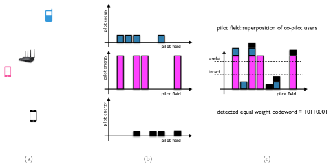
Figure 2: A qualitative example of the coded pilot threshold rule for $Q^{\prime}=8$ and three co-pilot users. a) geometry with one RRH and three users; b) individual equal-weight pilot fields after spatial matched filtering; c) received superposition and two-threshold mechanism. In this case, the pilot $q$ can be trusted.

II-C System Operation and Achievable Spectral Efficiency

For a sufficiently dense deployment of RRHs, each UE can be potentially served by several RRHs. The network layer routing ensures that the RRHs in the vicinity of any given UE $j$ have data packets in their queue, ready for transmission to user $j$. After receiving the UL pilot of the current TDD slot, RRH $k$ forms a list ${\cal U}_{k}$ of users (referred to as the active set of RRH $k$) that can be served in the corresponding DL data subslot. In particular, a user $j:u_{j}\in{\Phi}_{\rm u}^{(q)}$ is in the active set if: 1) RRH $k$ determines (by applying the aforementioned trusted pilot detection rule) that the corresponding pilot $q$ is trusted. Since an equal-weight codeword is uniquely assigned to the users in pilot group ${\cal C}_{q}$, the corresponding strong user $j:u_{j}\in{\Phi}_{\rm u}^{(q)}$ in the proximity of RRH $k$ is also identified; 2) RRH $k$ has a DL data packet ready to send to user $j$.

By construction, we have $0\leq|{\cal U}_{k}|\leq Q$ and we assume that the number of RRH antennas is $M\geq Q$, in compliance with the massive MIMO concept of more antennas than users [10]. The $k$-th RRH calculates the precoding vectors ${\bm{v}}_{k,j}$ for each user $j\in{\cal U}_{k}$ from its (trusted) channel estimates. We introduce the notation $\widehat{{\bf g}}_{k,j}=\widehat{{\bf g}}_{k}^{(q)}$ where user $j$ is the unique user in ${\cal U}_{k}$ associated to pilot group $q$. The precoder is obtained by using zero-forcing beamforming (ZFBF) as in [21]. Here, however, we consider unit-norm precoding vectors. These are obtained by first arranging the estimated channel vectors into the $M\times|{\cal U}_{k}|$ channel matrix $\widehat{{\bf G}}_{k}=\{\widehat{{\bf g}}_{k,j}:j\in{\cal U}_{k}\}$, then computing the Moore-Penrose pseudo-inverse matrix $\widehat{{\bf G}}_{k}^{\dagger}=\widehat{{\bf G}}_{k}(\widehat{{\bf G}}_{k}^{\sf H}\widehat{{\bf G}}_{k})^{-1}$, and finally letting ${\bm{v}}_{k,j}$ be the column of $\widehat{{\bf G}}_{k}^{\dagger}$ corresponding to $\widehat{{\bf g}}_{k,j}$, normalized by its magnitude.

Notice that a given user $j:u_{j}\in{\Phi}_{\rm u}^{(q)}$ may be in the active set of multiple RRHs. Since the RRHs make their own local decisions without coordination (apart from the implicit coordination induced by network layer routing), each RRH whose active set contains user $j$ will send simultaneously the same data packet to user $j$, achieving implicit macro-diversity. We let ${\cal A}_{j}=\{k:a_{k}\in{\Phi}_{\rm a},j\in{\cal U}_{k}\}$ denote the set of RRHs serving user $j$, and denote by ${\cal A}_{j}^{c}$ the complement set with respect to ${\Phi}_{\rm a}$. The DL received signal at user $j$ is given by

$$y_{j} =\left(\sum_{k\in{\cal A}_{j}}{\bf g}_{k,j}^{\sf H}{\bm{v}}_{k,j}\right)x_{j}+\sum_{k\in{\cal A}_{j}}{\bf g}_{k,j}^{\sf H}\left(\sum_{j^{\prime}\in{\cal U}_{k}:j^{\prime}\neq j}{\bm{v}}_{k,j^{\prime}}x_{j^{\prime}}\right)+\sum_{k\in{\cal A}^{c}_{j}}{\bf g}_{k,j}^{\sf H}\left(\sum_{j^{\prime}\in{\cal U}_{k}}{\bm{v}}_{k,j^{\prime}}x_{j^{\prime}}\right)+z_{j}$$ (9)

where the first term is the useful signal, the second and third terms correspond to the interference from RRHs serving user $j$ and RRHs not serving user $j$, respectively, while $z_{k}\sim{\cal C}{\cal N}(0,\sigma^{2}_{\rm\scriptscriptstyle N}/P_{\rm s}^{\rm fog})$ represents the AWGN with $P_{\rm s}^{\rm fog}$ the per-stream DL power and $\sigma^{2}_{\rm\scriptscriptstyle N}$ the noise variance. We assume unit-energy, zero-mean, and mutually statistically independent data symbols. Hence, the total transmit power of RRH $k$ in the current DL subslot is given by $|{\cal U}_{k}|P_{\rm s}^{\rm fog}$. When the RRH has no trusted pilots, it simply does not transmit anything thus achieving power savings in a seamless way (automatic shut-down in the absence of requested traffic). For future comparison with the baseline cellular system, the per-RRH average transmit power is given by $\mbox{\bb E}[|{\cal U}_{k}|]P_{\rm s}^{\rm fog}$.

We consider the ergodic spectral efficiency where ergodicity is with respect to the small scale fading, for fixed realization of ${\Phi}_{\rm u}$ (user positions) and ${\Phi}_{\rm a}$ (RRH positions). We start from the general achievable ergodic spectral efficiency expression for user $j$ [21]

$$C_{j}=\log_{2}\left(1+\frac{\left|\mbox{\bb E}[\mbox{useful}]\right|^{2}}{\frac{\sigma^{2}_{\rm\scriptscriptstyle N}}{P_{\rm s}^{\rm fog}}+{\rm Var}(\mbox{useful})+\mbox{\bb E}[|\mbox{interference}|^{2}]}\right)$$ (10)

and derive a compact expression that will be used in the next section for the stochastic geometry analysis. Before going into the ergodic rate analysis, it is convenient to distinguish between the contribution of non-copilot interference and that of co-pilot interference. To this purpose, we further partition the set of interfering RRHs ${\cal A}_{j}^{\rm c}$ into a set $\widetilde{{\cal A}}_{j}^{\rm c}$ of RRHs for which pilot $q$ is trusted, and a set $\overline{{\cal A}}_{j}^{\rm c}$ of RRHs for which pilot $q$ is untrusted. The non-copilot interference is due to all data streams transmitted by RRHs $k\in\overline{{\cal A}}_{j}^{\rm c}$ as well as all data streams from RRHs $k\in{\cal A}_{j}\cup\widetilde{{\cal A}}_{j}^{\rm c}$ except those associated to the channel estimate obtained from UL pilot $q$. The exact closed-form expression for an achievable ergodic rate in (10) is given by:

Proposition 1.

For the fog massive MIMO network model defined above, the following ergodic spectral efficiency is achievable by ZFBF:

$$C_{j}=\log_{2}\left(1+\frac{\left|\sum\limits_{k\in{\cal A}_{j}}\sqrt{\alpha_{k,j}\beta_{k,j}}\sqrt{M-|{\cal U}_{k}|+1}\right|^{2}}{\frac{\sigma^{2}_{\rm\scriptscriptstyle N}}{P_{\rm s}^{\rm fog}}-\sum\limits_{k\in{\cal A}_{j}\cup\widetilde{{\cal A}}_{j}^{\rm c}}\alpha_{k,j}\beta_{k,j}|{\cal U}_{k}|+\sum\limits_{k:a_{k}\in{\Phi}_{\rm a}}\beta_{k,j}|{\cal U}_{k}|+\sum\limits_{k\in\widetilde{{\cal A}}_{j}^{\rm c}}\alpha_{k,j}\beta_{k,j}(M-|{\cal U}_{k}|+1)}\right),$$ (11)

where

$$\alpha_{k,j}=\frac{\beta_{k,j}}{\sum_{j^{\prime}:u_{j^{\prime}}\in{\Phi}_{\rm u}^{(q)}}\beta_{k,j^{\prime}}+\frac{\sigma^{2}_{\rm\scriptscriptstyle N}}{P_{\rm u}Q}}$$ (12)

is the scaling coefficient in the conditional mean $\mbox{\bb E}[{\bf g}_{k,j}|\widehat{{\bf g}}_{k}^{(q)}]=\alpha_{k,j}\widehat{{\bf g}}_{k}^{(q)}$, and where $\widehat{{\bf g}}_{k}^{(q)}$ given in (3).

Proof.

Appendix A. ∎

It is important to notice that the MMSE scaling factors $\alpha_{k,j}$ appear in (11) uniquely as a product of the analysis, but have nothing to do with MMSE channel estimation. In fact, the channel estimates from the UL pilots are given by (3), which is simply a Least-Squares projection that does not assume any prior knowledge of the large-scale channel gains.

In order to obtain a simple expression, amenable to the stochastic geometry analysis of the next sections, we consider the limit $M\rightarrow\infty$ as in [10]. Notice that the coefficients $\alpha_{k,j}$ defined in (12) include the path coefficients of all UEs $j^{\prime}:u_{j^{\prime}}\in{\tilde{\Phi}}_{\rm u}^{(q)}$. These dependencies make the stochastic geometry analysis intractable. However, we notice that the denominator of the fraction in the RHS of (12) contains a single strong channel gain and many other weak channel gains, as a consequence of the trusted pilot detection rule. By the symmetry of the PPP, the mean value of this denominator is independent of the RRH index $k\in{\cal A}_{j}\cup\widetilde{{\cal A}}_{j}^{\rm c}$. Furthermore, these denominators should be close to their mean value and therefore, up to small statistical fluctuations, all approximately equal. With this approximation, letting $M\rightarrow\infty$ in (11), we obtain the large-$M$ spectral efficiency expression

$$C_{j}^{\infty}=\log\left(1+\frac{\left|\sum_{k\in{\cal A}_{j}}\beta_{k,j}\right|^{2}}{\sum_{k\in\widetilde{{\cal A}}_{j}^{\rm c}}\beta_{k,j}^{2}}\right),$$ (13)

which is well-known from [10], with the only difference of the coherent combining of multiple transmissions in the numerator in the case $|{\cal A}_{j}|\geq 1$ for the already discussed inherent macro-diversity of the scheme.

III Main Analytical Results

First, we present analytical expressions for the active co-pilot user density and the active RRH density. Then, we derive the approximate expression for the spatially averaged spectral efficiency in the limit of $M\to\infty$.

III-A Active Co-pilot User Density

Recall from Section II-B that each RRH identifies its trusted pilots based on a decision rule involving the two thresholds $\tau_{\rm useful}$ and $\tau_{\rm interf}$. Assuming that the large-scale channel gain coefficients appearing in (7) are decreasing functions of the distance between UE and RRH with a radial symmetry, for the sake of the stochastic geometry analysis we shall approximate the trusted pilot detection rule with a purely geometric rule. Namely, the thresholds $\tau_{\rm useful}$ and $\tau_{\rm interf}$ correspond to two circular regions each RRH referred to in the following as the coverage disk and the protection disk with radii $R_{\rm in}$ and $R_{\rm out}=(1+\epsilon)\cdot R_{\rm in}$, with $\epsilon\geq 0$, respectively.

Without loss of generality, we can place a reference user at $u_{0}$, associated to a given pilot group ${\cal C}_{q}$, referred to for simplicity as “pilot $q$”. The reference user can be served by a RRH at location $a_{0}$ if an only if $a_{0}\in{\mathcal{B}}_{u_{0}}(R_{\rm in})$ (the RRH is within the inner radius of the reference user) and $a_{0}\notin{\mathcal{B}}_{u_{j}}(R_{\rm out})$ for all $u_{j}\in{\Phi}_{\rm u}^{(q)}\setminus u_{0}$ (the RRH is outside the protection radius of all other users associated to the same pilot $q$). We say that a user at $u_{0}$ is “allowed” to receive in the DL if there is at least one RRH at some position $a_{0}$ meeting the above condition. Let $\theta$ denote the fraction of the disk ${\mathcal{B}}_{u_{0}}(R_{\rm in})$ uncovered by the union of disks $\bigcup_{u_{j}\in{\Phi}_{\rm u}^{(q)}\setminus u_{0}}{\mathcal{B}}_{u_{j}}(R_{\rm out})$. Then, conditioned on the uncovered fraction $\theta$, we have

$${\mathbb{P}}\left(u_{0}\,\textnormal{ is allowed}\,|\theta\right) =1-e^{{\lambda}_{\rm a}\pi R_{\rm in}^{2}\theta}$$ (14)

which follows from the void probability of the PPP ${\Phi}_{\rm a}$ (the probability that there exists no point of the PPP [22]) in the uncovered region of area $\pi R_{\rm in}^{2}\theta$. Averaging (14) over $\theta$ gives

$${\mathbb{P}}\left(u_{0}\,\textnormal{ is allowed}\right) =\int_{0}^{1}\left(1-e^{{\lambda}_{\rm a}\pi R_{\rm in}^{2}\theta}\right)\,f_{\theta}(\theta)\,{\mathrm{d}}\theta$$ (15)

where $f_{\theta}(\cdot)$ denotes the probability density function (PDF) of the uncovered area fraction $\theta$. As a result, the mean active co-pilot user density is given by

$${\tilde{\lambda}} =\lambda\,{\mathbb{P}}\left(u_{0}\,\textnormal{ is allowed}\right)=\lambda\int_{0}^{1}\left(1-e^{{\lambda}_{\rm a}\pi R_{\rm in}^{2}\theta}\right)\,f_{\theta}(\theta)\,{\mathrm{d}}\theta.$$ (16)

In light of the fact that there are no available tractable expressions for the PDF $f_{\theta}(\cdot)$, a possible semi-analytic approach consists of using Monte-Carlo simulation to calculate $f_{\theta}(\cdot)$ for any given ratio of ${\lambda}_{\rm a}/\lambda$ and evaluate the integral in (14). As an alternative, in order to gain analytical insight, we extend the approximation proposed in [16] to calculate $f_{\theta}(\cdot)$ to the case $R_{\rm in}\leq R_{\rm out}$. The accuracy of this approximation is examined later in the section (cf. Example 1). Using this approach, $f_{\theta}(\cdot)$ can be approximated by a mixed-type PDF formed by the convex combination of a uniform PDF, a point mass at $\theta=0$, and a point mass at $\theta=1$. The resulting approximated PDF is given by (cf. Appendix B)

$${\hat{f}}_{\theta}(\theta) =\begin{cases}1+e^{-\pi\lambda(R_{\rm out}+R_{\rm in})^{2}}-2\,e^{-\pi\lambda R_{\rm out}^{2}}&\quad\textnormal{point mass at}\,\,\theta=0\\ 2\left(e^{-\pi\lambda R_{\rm out}^{2}}-e^{-\pi\lambda(R_{\rm out}+R_{\rm in})^{2}}\right)&\quad 0<\theta<1\\ e^{-\pi\lambda(R_{\rm out}+R_{\rm in})^{2}}&\quad\textnormal{point mass at}\,\,\theta=1\end{cases}$$ (17)

$\lozenge$

Using (17) in (16) yields the closed-form approximation for the active co-pilot user density:

$${\tilde{\lambda}} \approx 2\lambda\left(e^{-\pi\lambda R_{\rm out}^{2}}-e^{-\pi\lambda(R_{\rm in}+R_{\rm out})^{2}}\right)\left(1-\frac{1-e^{-\pi{\lambda}_{\rm a}R_{\rm in}^{2}}}{\pi{\lambda}_{\rm a}R_{\rm in}^{2}}\right)+\lambda\left(\frac{1-e^{-\pi{\lambda}_{\rm a}R_{\rm in}^{2}}}{e^{\pi\lambda(R_{\rm in}+R_{\rm out})^{2}}}\right).$$ (18)

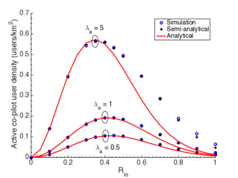
Figure 3: Active co-pilot user density v. $R_{\rm in}$ for ${\lambda}_{\rm a}=0.5$ RRHs per unit area, ${\lambda}_{\rm a}=1$ RRH per unit area and ${\lambda}_{\rm a}=5$ RRHs per unit area, with ${\lambda}=1$ user per unit area and $R_{\rm out}=1.25R_{\rm in}$.

Example 1.

Fig. 3 compares, as function of $R_{\rm in}$, the active co-pilot user density ${\tilde{\lambda}}$ estimated via (16) and (18) against the simulated counterpart for user density ${\lambda}=1$ user per unit area, and different RRH densities ${\lambda}_{\rm a}=0.5$ RRHs per unit area, ${\lambda}_{\rm a}=1$ RRH per unit area, and ${\lambda}_{\rm a}=5$ RRHs per unit area, and with $R_{\rm out}=1.25R_{\rm in}$. These settings span the three possible network scenarios of ${\lambda}_{\rm a}<{\lambda}$, ${\lambda}_{\rm a}={\lambda}$ and ${\lambda}_{\rm a}>{\lambda}$, respectively. As seen in Fig. 3, the value of $R_{\rm in}$ maximizing the active co-pilot user density decreases with ${\lambda}_{\rm a}$ (when ${\lambda}$ is fixed). The semi-analytic approach is also shown. As said before, this approach is very accurate and significantly more computationally efficient than the full Monte-Carlo system simulation. As can be seen in Fig. 3, a very satisfactory agreement is observed when $R_{\rm in}$ is less than or equal to the value that maximizes ${\tilde{\lambda}}$. If $R_{\rm in}$ is beyond the value that maximizes ${\tilde{\lambda}}$, then (18) underestimates the active co-pilot user density and this estimation error is noticeable when ${\lambda}_{\rm a}>1$. Similar agreement has been observed for other values of parameters. Therefore, it is reasonable to utilize (18) as a proxy to optimize the active co-pilot user density up to $R_{\rm in}$ that maximizes ${\tilde{\lambda}}$. $\lozenge$

III-B Active RRH Density and Transmit Power

The RRH at $a_{0}$ has an active user corresponding to the pilot under consideration if and only if there exists only one user in its coverage disk, i.e., $\exists u_{0}\in{\mathcal{B}}_{a_{0}}(R_{\rm in})\cap{\Phi}_{\rm u}^{(q)}$ and no other users in its protection disk, i.e., ${\mathcal{B}}_{a_{0}}(R_{\rm out})\cap{\Phi}_{\rm u}^{(q)}\setminus\{u_{o}\}=\emptyset$. Denoting by ${\tilde{\Phi}}_{\rm a}^{(q)}$ the locations of active RRHs corresponding to the pilot and by ${\tilde{\lambda}}_{\rm a}^{(q)}$ the density of active RRHs, we can express

$${\tilde{\lambda}}_{\rm a}^{(q)} ={\lambda}_{\rm a}\,{\mathbb{P}}\left({\Phi}_{\rm u}^{(q)}({\mathcal{B}}_{a_{0}}(R_{\rm in}))=1\right)\,{\mathbb{P}}\left({\Phi}_{\rm u}^{(q)}({\mathcal{B}}_{a_{0}}(R_{\rm out})\setminus{\mathcal{B}}_{a_{0}}(R_{\rm in}))=0\right)$$ (19)

$$={\lambda}_{\rm a}\,{\lambda}\pi R_{\rm in}^{2}\,e^{-\pi{\lambda}R_{\rm out}^{2}}$$ (20)

where for a region $B\subseteq\mbox{\bb R}^{2}$ we use the short-hand notation ${\Phi}_{\rm u}^{(q)}(B)=|{\Phi}_{\rm u}^{(q)}\cap B|$, and where (20) follows from the well-known property of PPPs [22] ${\mathbb{P}}\left({\Phi}_{\rm u}^{(q)}(B)=n\right)=e^{-{\lambda}|B|}\frac{\left({\lambda}|B|\right)^{n}}{n!}$.

It is also immediate to express the average number of users served by the RRH as

$${\mathbb{E}}[|{\cal U}_{0}|] =Q{\lambda}\pi R_{\rm in}^{2}\,e^{-\pi{\lambda}R_{\rm out}^{2}}.$$ (21)

Multiplying by the per-stream power $P_{\rm s}^{\rm fog}$, we obtain the average RRH transmit power as

$$P_{\rm a} =P_{\rm s}^{\rm fog}Q\,{\lambda}\pi R_{\rm in}^{2}\,e^{-\pi{\lambda}R_{\rm out}^{2}}.$$ (22)

III-C Spectral Efficiency in the Large Antenna Regime

Let $\eta$ denote the propagation pathloss exponent and $r_{k,j}=|a_{k}-u_{j}|$ the distance between RRH $k$ and UE $j$. We assume that the large-scale channel gains obey the usual distance-based polynomial decay law $\beta_{k,j}=r_{k,j}^{-\eta}$. Using this in (13), the ergodic spectral efficiency of the typical user can be written as

$$C_{0}^{\infty}=\log_{2}\left(1+\frac{\sigma^{2}_{\rm\scriptscriptstyle S}}{\sigma^{2}_{\rm\scriptscriptstyle I}}\right),$$ (23)

where $\sigma^{2}_{\rm\scriptscriptstyle S}=\left|\sum_{k\in{\mathcal{A}}_{0}}r_{k,0}^{-\eta}\right|^{2}$ and $\sigma^{2}_{\rm\scriptscriptstyle I}=\sum_{k\in\widetilde{{\cal A}}_{0}^{\rm c}}r_{k,0}^{-2\,\eta}$. In turn, (23) involves multiple levels of randomness through $|{\cal A}_{0}|$, $r_{k,0}\,\forall k\in{\cal A}_{0}$, and $r_{k,0}\,\forall k\in\widetilde{{\cal A}}_{0}^{\rm c}$. We marginalize the spectral efficiency $C_{0}^{\infty}$ in multiple steps to characterize the spatially averaged per-user spectral efficiency, given by

$${\bar{C}}_{0}^{\infty} =\sum_{n=1}^{N}{\mathbb{P}}\left(|{\mathcal{A}}_{0}|=n\Big{|}|{\mathcal{A}}_{0}|>0\right){\mathbb{E}}\left[{\mathbb{E}}\left[\log_{2}\left(1+\frac{\sigma^{2}_{\rm\scriptscriptstyle S}}{\sigma^{2}_{\rm\scriptscriptstyle I}}\right)|\sigma^{2}_{\rm\scriptscriptstyle S}\right]\right].$$ (24)

The value of $N$ in (24) is chosen sufficiently large such that ${\mathbb{P}}\left(|{\mathcal{A}}_{0}|=N+1\right)$ is negligible, the inner expectation is over the interference (i.e., $r_{0,k}\,\forall k\in\widetilde{{\mathcal{A}}}_{0}^{\rm c}$) while the outer expectation is over the signal (i.e., $r_{0,k}\,\forall k\in{{\cal A}}_{0}$).

The probability that the number of RRHs in the uncovered area equals $n$ can be written as

$${\mathbb{P}}\left(|{\mathcal{A}}_{0}|=n\Big{|}|{\mathcal{A}}_{0}|>0\right) =\frac{\int\limits_{0}^{1}{\mathbb{P}}\left({\Phi}_{\rm a}(\theta{\mathcal{B}}(0,R_{\rm in}))=n\right)f_{\theta}(\theta)\,{\mathrm{d}}\theta}{\sum\limits_{n^{\prime}=1}^{N}\int\limits_{0}^{1}{\mathbb{P}}\left({\Phi}_{\rm a}(\theta{\mathcal{B}}(0,R_{\rm in}))=n^{\prime}\right)f_{\theta}(\theta)\,{\mathrm{d}}\theta}.$$ (25)

This can be computed either by using the PDF of the uncovered area fraction $f_{\theta}(\theta)$ obtained via simulation (semi-analytic method), or using approximation (17). By invoking (17), the integral in (25) is given by

$$\!\!\!\!\!\!\int\limits_{0}^{1}{\mathbb{P}}\left({\Phi}_{\rm a}(\theta{\mathcal{B}}(0,R_{\rm in}))=n\right)f_{\theta}(\theta)\,{\mathrm{d}}\theta$$

$$=\frac{2}{n!\,\pi{\lambda}_{\rm a}R_{\rm in}^{2}}\left(e^{-\pi{\lambda}R_{\rm out}^{2}}-e^{-\pi{\lambda}(R_{\rm out}+R_{\rm in})^{2}}\right)e^{-\pi{\lambda}(R_{\rm out}^{2}+(R_{\rm out}+R_{\rm in})^{2})}\bar{\Gamma}\left(n+1,\pi R_{\rm in}^{2}{\lambda}_{\rm a}\right)$$

$$\quad+e^{-\pi{\lambda}_{\rm a}R_{\rm in}^{2}-\pi{\lambda}(R_{\rm out}+R_{\rm in})^{2}}\frac{(\pi{\lambda}_{\rm a}R_{\rm in}^{2})^{n}}{n!}.$$ (26)

where $\bar{\Gamma}(\cdot,\cdot)$ is the lower incomplete Gamma function.

Next, by virtue of [23, Lemma 1], the inner expectation in (24) can be expressed as

$${\mathbb{E}}\left[\log_{2}\left(1+\frac{\sigma^{2}_{\rm\scriptscriptstyle S}}{\sigma^{2}_{\rm\scriptscriptstyle I}}\right)|\sigma^{2}_{\rm\scriptscriptstyle S}\right] ={\mathbb{E}}\left[\int_{0}^{\infty}\frac{1}{\gamma}\left(e^{-\gamma\,\sigma^{2}_{\rm\scriptscriptstyle I}}-e^{-\gamma(\sigma^{2}_{\rm\scriptscriptstyle I}+\sigma^{2}_{\rm\scriptscriptstyle S})}\right)\,{\mathrm{d}}\gamma\right]$$ (27)

$$=\int_{0}^{\infty}\frac{1}{\gamma}\left({\mathbb{E}}\left[e^{-\gamma\,\sigma^{2}_{\rm\scriptscriptstyle I}}\right]-{\mathbb{E}}\left[e^{-\gamma\,\sigma^{2}_{\rm\scriptscriptstyle I}}\right]e^{-\gamma\,\sigma^{2}_{\rm\scriptscriptstyle S}}\right)\,{\mathrm{d}}\gamma$$ (28)

Due to the activation of the RRH through the on-the-fly pilot contamination control mechanism (cf. Section II-B), the interfering RRH locations in the downlink (i.e., appearing in the set $\widetilde{{\cal A}}^{\rm c}_{0}$) are dependent on their user locations and violate the PPP condition. In order to overcome this obstacle, we borrow a modeling assumption that was shown to be tight in different scenarios [24, 25] and whose validity for our purposes is examined later in Example 2.

Assumption 1: The RRH locations outside the receiver’s protection disk ${\mathcal{B}}_{u_{0}}(R_{\rm out})$ belong to another independent PPP with matched density ${\tilde{\lambda}}_{\rm a}^{(q)}$ (cf. (20)). $\lozenge$

Under Assumption 1, the expectation of $e^{-\gamma\,\sigma^{2}_{\rm\scriptscriptstyle I}}$ over this PPP yields

$${\mathbb{E}}\left[e^{-\gamma\,\sigma^{2}_{\rm\scriptscriptstyle I}}\right] ={\mathbb{E}}\left[\exp\left(-\gamma\,\sum_{k\in\widetilde{{\cal A}}_{0}^{\rm c}}r_{k,0}^{-2\eta}\right)\right]$$ (29)

$$=\exp\left(-2\pi{\tilde{\lambda}}_{\rm a}^{(q)}\int_{R_{\rm out}}^{\infty}\left(1-e^{-\gamma\,r^{-2\eta}}\right)r\,{\mathrm{d}}r\right)$$ (30)

$$=\exp\left(\pi{\tilde{\lambda}}_{\rm a}^{(q)}R_{\rm out}^{2}+\frac{\pi{\tilde{\lambda}}_{\rm a}^{(q)}\gamma^{\frac{1}{\eta}}}{\eta}\bar{\Gamma}\left(-\frac{1}{\eta},\frac{\gamma}{R_{\rm out}^{2\eta}}\right)\right)$$ (31)

where (30) follows from the PGFL (probability generating functional) of the PPP [22] and (31) follows from the change of variable $\gamma\,r^{-2\eta}\to r^{\prime}$ and then solving the integral in (30).

Then, the remaining randomness in $C_{0}^{\infty}$ is due to $\sigma^{2}_{\rm\scriptscriptstyle S}$. Conditioned on $|{\mathcal{A}}_{0}|=n$, the distance from the intended RRH locations to the user can be ordered as $r_{0,0},r_{1,0},\ldots,r_{n-1,0}$, where $r_{n-1,0}$ is the distance corresponding to the $n$th strongest serving RRH. Then, we have

$$\sigma^{2}_{\rm\scriptscriptstyle S} =\left(\sum_{k=0}^{n-1}r_{k,0}^{-\eta}\right)^{2}.$$ (32)

Here, the intended RRHs are uniformly distributed in the uncovered region of ${\mathcal{B}}_{0}(R_{\rm in})$ that is arbitrarily shaped and hence their distances are not tractable in general. Again, we make a modeling assumption (the accuracy of which is also validated in Example 2) in order to proceed with the closed-form analysis.

Assumption 2: The serving RRHs are uniformly distributed in the whole disk ${\mathcal{B}}_{0}(R_{\rm in})$ and the distances $\{r_{k,0}\}_{k=0}^{n-1}$ are replaced with their expected values. $\lozenge$

Under Assumption 2, we have

$$\sigma^{2}_{\rm\scriptscriptstyle S} \approx\left(\sum_{k=0}^{n-1}{\left({\mathbb{E}}\left[r_{k,0}\right]\right)}^{-\eta}\right)^{2}$$ (33)

where the expected value of the distance between the user and the $m$th closest point when $|{\mathcal{A}}_{0}|=n$ is

$${\mathbb{E}}\left[r_{m,0}\right] =R_{\rm in}\frac{\Gamma(m+\frac{3}{2})\Gamma(n+1)}{\Gamma(m+1)\Gamma(n+\frac{3}{2})}\qquad m=0,1,\ldots,n-1$$ (34)

which leads to a deterministic value for $\sigma^{2}_{\rm\scriptscriptstyle S}$ in (33) and thus avoids the outer expectation in (24). Finally an approximation for ${\bar{C}}_{0}^{\infty}$ can be obtained by plugging (25), (28), (31), (33) and (34) in (24).

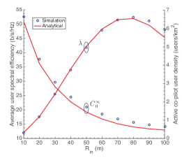
(a) Average user spectral efficiency

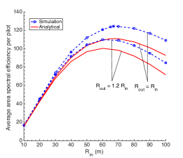
(b) Average area spectral efficiency per pilot

Figure 4: Spectral efficiency v. $R_{\rm in}$ for ${\lambda}_{\rm a}=31.8\,\textnormal{RRHs/ km}^{2}$, ${\lambda}={\lambda}_{\rm a}$, $Q=40$ and $\eta=3.75$.

Example 2.

Consider RRH density ${\lambda}_{\rm a}=31.8\,\textnormal{RRHs/km}^{2}$ (corresponding to an average of one RRH per circular cell of radius 100 m), ${\lambda}={\lambda}_{\rm a}$, $\eta=3.75$, and $Q=40$. Fig. 4 compares the closed-form approximation ${\bar{C}}_{0}^{\infty}$ in (24) based on (17) and Assumptions 1-2 with its simulated counterpart for protection radius set to $R_{\rm out}=1.2R_{\rm in}$. The simulated result corresponds to explicit computation of the spectral efficiency without any modeling assumptions, computed through lengthy Monte-Carlo over many network realizations. As the figure reveals, the match between analysis and simulation is satisfactory, thereby supporting the validity of the modeling assumptions. From Fig. 4, we notice that the user spectral efficiency decreases with coverage and protection radii. This is because of the increase in the aggregate interference from the active RRHs with $R_{\rm in}$ (cf. (20)). However, low values of $R_{\rm in}$ yield small spatial pilot reuse (cf. Fig. 4). This in turn reduces the spatially averaged area spectral efficiency $(\textnormal{b/s/Hz/km}^{2})$ per pilot, defined by ${\bar{C}}^{\rm\scriptscriptstyle pilot}\triangleq{\tilde{\lambda}}\,{\bar{C}}_{0}^{\infty}$. Therefore, $R_{\rm in}$ must optimized by striking a good tradeoff between pilot reuse and per-user spectral efficiency.

Shown in Fig. 4 is ${\bar{C}}^{\rm\scriptscriptstyle pilot}$ with ${\tilde{\lambda}}$ given by (18) and ${\bar{R}}_{0}$ given by (24)), alongside the simulation counterpart. The average area spectral efficiency per pilot ${\bar{C}}^{\rm\scriptscriptstyle pilot}$ is uniformly superior with $R_{\rm out}=R_{\rm in}$ over $R_{\rm out}=1.2R_{\rm in}$. Again, the match is satisfactory with error due to the modeling assumptions in the range of 5-12% for the typical values of $R_{\rm in}$. Therefore, it is reasonable to consider the analytical approximation of ${\bar{C}}^{\rm\scriptscriptstyle pilot}$ as a proxy to tune the radii of the pilot detection rule, while the exact value of the area spectral efficiency per pilot can be obtained by conducting simulations for specific values of $R_{\rm in}$. $\lozenge$

We conclude by mentioning that, since the signals for different pilots $q$ are completely decoupled by the massive MIMO in the regime $M\rightarrow\infty$, the total average area spectral efficiency (b/s/Hz per unit area) of the fog massive MIMO system operating with $Q$ pilot groups is simply given by ${\mathcal{C}}^{\rm\scriptscriptstyle fog}=Q{\bar{C}}^{\rm\scriptscriptstyle pilot}$.

IV Cellular Massive MIMO System

In this section, we briefly present the system model and achievable spectral efficiency analysis for a baseline cellular massive MIMO system that we use as a term of comparison for our fog massive MIMO system. Differently from the classical works on massive MIMO (e.g., [10, 26, 27, 21]), which have mostly considered regular (e.g., hexagonal) cells and integer pilot reuse factors, here we consider UEs and BSs placed according to the PPPs ${\Phi}_{\rm u}$ and ${\Phi}_{\rm a}$, respectively, and a statistical fractional UL pilot reuse scheme, which is more representative of a “small-cell” deployment.

IV-A System Configuration

In the considered cellular massive MIMO system, each user is served by the closest BS, resulting in the standard Voronoi-tessellated network geometry. As for the fog system, we assume a coherence block of $T$ dimensions, $L$ of which are dedicated to UL mutually orthogonal pilot sequences. A reference BS at $a_{0}$ serves $|{\cal U}_{0}|=\min(|{\mathcal{V}}_{0}|,N_{\rm p})$ users in the DL, where $|{\mathcal{V}}_{0}|$ denotes the number of users in its Voronoi cell and $0<N_{\rm p}\leq L$ is a parameter that controls the (fractional) pilot reuse across the cells. Letting $N_{\rm p}=L$ yields reuse 1 (all pilots are used in all cells, for sufficiently large user density). Otherwise, for $N_{\rm p}<L$, we assume that $|{\cal U}_{0}|$ out of the $L$ available pilots are selected at random and independently across the cells. This implies that the allocation of pilots to users is done without inter-cell coordination. Yet, all users served in the same cell use mutually orthogonal pilots. The per-stream power in cellular system $P_{\rm s}^{\rm cell}$ is fixed such that the average power transmitted by each BS is same as the average power of the RRHs of the fog system. Using the expression for the average number of users served by a BS given in Appendix C, the per-stream power in the cellular system is related to the average BS power $P_{\rm a}$ as $P_{\rm s}^{\rm cell}=P_{\rm a}/{\mathbb{E}}\left[|{\cal U}_{0}|\right]$. Furthermore, the location of BSs serving users associate to a specific pilot $q\in[L]$ can be viewed as a thinned version of the original PPP, denoted hereafter by ${\tilde{\Phi}}_{\rm a}^{(q)}$, whose density equals ${p_{\rm a}}{\lambda}_{\rm a}$. The thinning probability ${p_{\rm a}}$ equals the probability that the pilot is assigned to one of the ${\cal U}_{0}$ users, which can be computed as

$${p_{\rm a}} =\frac{N_{\rm p}}{L}+\frac{1}{L}\sum_{\ell=0}^{N_{\rm p}-1}(\ell-N_{\rm p})\,\frac{\Gamma(\ell+c)}{\Gamma(\ell+1)\Gamma(c)}\frac{({\lambda}_{\rm u})^{\ell}(c{\lambda}_{\rm a})^{c}}{(c{\lambda}_{\rm a}+{\lambda}_{\rm u})^{\ell+c}}.$$ (35)

IV-B Spectral Efficiency in the Large Antenna Regime

Following the similar approach of fog massive MIMO (cf. Section II-C), one can derive the ergodic user spectral efficiency of cellular massive MIMO, where in this case $|{\cal A}_{j}|=1$ for any served user at $u_{j}$. For the sake of brevity, in this section we directly consider the spectral efficiency in the limit of $M\to\infty$ and obtain its spatial averaged quantity. The SIR experienced by a typical user located at $u_{0}$, served by a BS located at $a_{0}$, is expressed as

$${\mathrm{SIR}}_{0} =\frac{\beta_{0,0}^{2}}{\sum\limits_{k\in\widetilde{{\cal A}}_{0}^{\rm c}}\beta_{k,0}^{2}}=\frac{r_{0,0}^{-2\,\eta}}{r_{1,0}^{-2\,\eta}+\sum\limits_{k\in\widetilde{{\cal A}}_{0}^{\rm c}\setminus\{1\}}r_{0,k}^{-2\,\eta}}$$ (36)

where in (36) $r_{1,0}$ denotes the distance from the user at $u_{0}$ to the strongest interfering BS located at $a_{1}\in{\tilde{\Phi}}_{\rm a}^{(q)}$. At this point, as in [28, 29, 25], we invoke the modeling assumption introduced in Section III-C, i.e., the locations of interfering BSs outside ${\mathcal{B}}_{u_{0}}(r_{1,0})$ belongs to a PPP with scaled-down density ${p_{\rm a}}{\lambda}_{\rm a}$ and replace the corresponding collective interference term with its spatial average. This yields

$${\mathrm{SIR}}_{0} \approx\frac{r_{0,0}^{-2\,\eta}}{r_{1,0}^{-2\,\eta}+\frac{\pi{\lambda}_{\rm a}{p_{\rm a}}}{\eta-1}r_{1,0}^{2-2\eta}}=\frac{\delta_{0}^{2\eta}}{1+\frac{\pi{\lambda}_{\rm a}{p_{\rm a}}}{\eta-1}r_{1,0}^{2}},$$ (37)

where (37) follows by replacing the second term in the denominator of (36) with its expectation computed applying Campbell’s theorem and by introducing $\delta_{0}=r_{1,0}/r_{0,0}>1$.

Next, the average user spectral efficiency in the cellular massive MIMO network can be written as

$${\bar{C}}_{0}^{\infty} =\int_{1}^{\infty}\int_{0}^{\infty}\log_{2}\left(1+\frac{\delta_{0}^{2\eta}}{1+\frac{\pi{\lambda}_{\rm a}{p_{\rm a}}}{\eta-1}r_{1,0}^{2}}\right)f_{r_{1,0},\delta_{0}}(r_{1,0},\delta_{0})\,{\mathrm{d}}r_{1,0}{\mathrm{d}}\delta_{0}$$ (38)

where the PDF $f_{r_{1,0},\delta_{0}}(\cdot,\cdot)$ is given by

$$f_{r_{1,0},\delta_{0}}(r_{1,0},\delta_{0}) ={p_{\rm a}}(2\pi{\lambda}_{\rm a})^{2}\left(\frac{r_{1,0}}{\delta_{0}}\right)^{3}e^{-\pi{\lambda}_{\rm a}r_{1,0}^{2}\left({p_{\rm a}}+\frac{1-{p_{\rm a}}}{\delta_{0}^{2}}\right)}.$$ (39)

obtained by applying [30, Lemma 1]. We can obtain the aggregate average spectral efficiency of all the users of a cell by scaling the average user spectral efficiency ${\bar{C}}_{0}^{\infty}$ by the average number of users served by each BS. Consequently, the total average area spectral efficiency of the cellular massive MIMO system equals

$${\mathcal{C}}^{\rm\scriptscriptstyle cellular} ={\lambda}_{\rm a}{\mathbb{E}}[|{\cal U}_{0}|]\,{\bar{C}}_{0}^{\infty}.$$ (40)

where ${\bar{C}}_{0}^{\infty}$ is given in (38) and ${\mathbb{E}}[|{\cal U}_{0}|]$ is given in Appendix C.

We tested the above approximated analytical expressions against the full system Monte Carlo simulation (cf. Example 3), with excellent agreement.

TABLE I: Average User and Area Spectral Efficiencies of Cellular Massive MIMO

$N_{\rm p}$	${\bar{C}}_{0}^{\infty}$ (b/s/Hz)		${\mathcal{C}}^{\rm\scriptscriptstyle cellular}$ ($\textnormal{b/s/Hz/km}^{2}$)
	Analytical	Simulation	Analytical	Simulation
10	10.69	10.78	2587.9	2613.5
20	9.73	9.74	2998.2	3013.5
30	9.62	9.69	3051.5	3104.5
40	9.60	9.70	3056.9	3118.1

Example 3.

Consider ${\lambda}_{\rm a}=31.8\,\textnormal{RRHs/km}^{2}$, ${\lambda}_{\rm u}=10{\lambda}_{\rm a}$, $L=40$ and $\eta=3.75$, yielding ${p_{\rm a}}=0.25$. Shown in Table. I is a comparison of ${\bar{C}}_{0}^{\infty}$ (cf. (38)) and ${\mathcal{C}}^{\rm\scriptscriptstyle cellular}$ (cf. (40)) against their simulated counterparts. As can be seen, the area spectral efficiency increases with $N_{\rm p}$, which indicate that it is beneficial to utilize all the available orthogonal pilots to serve the maximum number of users (for the RRH and user densities chosen in this example).

V Performance Evaluation

With the theoretical framework developed in the previous sections, we now proceed to evaluate the performance of optimized fog massive MIMO system and contrast it with the cellular massive MIMO baseline. In fog massive MIMO, we assume $\epsilon=0$ (i.e., $R_{\rm out}=R_{\rm in}$) and pilot dimension $L=60$ where the UL pilot codebook is formed as described in Section II-A, with $Q=40$ and $Q^{\prime}=20$. In cellular massive MIMO, we consider $L=60$ orthogonal pilot sequences of dimension $60$ and $N_{\rm p}=L$, which maximizes the area spectral efficiency while minimizing the outage probability. We choose ${\lambda}_{\rm a}=31.8\,\textnormal{RRHs/ km}^{2}$, $\eta=3.75$ and ${\lambda}_{\rm u}=Q\lambda$ for both the fog and cellular massive MIMO systems. In all the following results, the pilot overhead is not taken into account. Depending on the number of signal dimensions available per slot $T$, the spectral efficiencies of fog and cellular massive MIMO systems should be scaled by the pilot overhead factor $(1-\frac{L}{T})$.

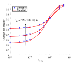
(a) Outage probability

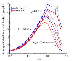
(b) Average area spectral efficiency per pilot

Figure 5: Performance of fog massive MIMO as function of ${\lambda}/{\lambda}_{\rm a}$ with $R_{\rm in}=80$ m, $R_{\rm in}=100$ m and $R_{\rm in}=120$ m, $\epsilon=0$, ${\lambda}_{\rm a}=31.8\,\textnormal{RRHs/ km}^{2}$, and $\eta=3.75$.

Example 4.

Fig. 5 shows, as function of ${\lambda}/{\lambda}_{\rm a}$, the outage probability in a fog massive MIMO network, which is defined as the probability of the event that there is no serving RRH in within $R_{\rm in}$ centered around the user, i.e., $P_{\rm out}=\mbox{\bb P}(B_{\rm\scriptscriptstyle c}(0,R_{\rm in})\cap{\Phi}_{\rm a}=\emptyset)$, while Fig. 5 shows the corresponding average area spectral efficiency per pilot. We compare different choices $R_{\rm in}=80$ m, $R_{\rm in}=100$ m and $R_{\rm in}=120$ m of the coverage radius. As seen in Fig. 5, the outage probability decreases with $R_{\rm in}$ at low values of ${\lambda}/{\lambda}_{\rm a}$, while it increases with $R_{\rm in}$ at high values of ${\lambda}/{\lambda}_{\rm a}$. As anticipated before, for a given value of $R_{\rm in}$, the area spectral efficiency per pilot (cf. Fig. 5) progressively increases with ${\lambda}/{\lambda}_{\rm a}$ and eventually decreases at higher values of ${\lambda}/{\lambda}_{\rm a}$ due to the excessive number of pilot collisions, essentially preventing most users to be served by any RRH. $\lozenge$

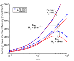
(a) Average area spectral efficiency

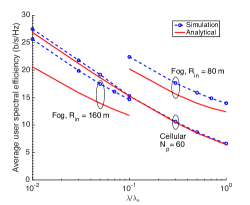
(b) Average user spectral efficiency

Figure 6: Performance evaluation of fog and cellular massive MIMO as function of ${\lambda}/{\lambda}_{\rm a}$ with $M\to\infty$, ${\lambda}_{\rm a}=31.8\,\textnormal{RRHs/ km}^{2}$, ${\lambda}_{\rm u}=Q\lambda$, $Q=40$, $Q^{\prime}=20$, $L=60$, $\eta=3.75$, $\epsilon=0$ and $N_{\rm p}=60$.

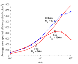
(a) Average area spectral efficiency

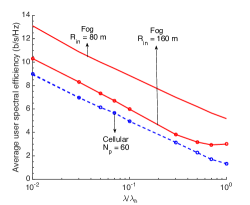
(b) Average user spectral efficiency

Figure 7: Performance evaluation of fog and cellular massive MIMO as function of ${\lambda}/{\lambda}_{\rm a}$ with $M=64$, ${\lambda}_{\rm a}=31.8\,\textnormal{RRHs/ km}^{2}$, ${\lambda}_{\rm u}=Q\lambda$, $Q=40$, $Q^{\prime}=20$, $L=60$, $\eta=3.75$, $\epsilon=0$ and $N_{\rm p}=60$.

Example 5.

Fig. 6 compares, as function of ${\lambda}/{\lambda}_{\rm a}$, the average area spectral efficiencies of fog and cellular massive MIMO systems. The corresponding user spectral efficiencies (restricted to users that are effectively served, i.e., not in outage) are shown in Fig. 6. For large coverage radius ($R_{\rm in}=160$m), the outage probability is around $10-20$% for ${\lambda}/{\lambda}_{\rm a}\in[0.01,0.1]$, and the resulting average area spectral efficiency is comparable ($15-25$% lower) to its cellular counterpart. A smaller coverage radius ($R_{\rm in}=80$ m) outperforms the larger radius for higher user density ${\lambda}/{\lambda}_{\rm a}\geq 0.3$. $\lozenge$

Example 6.

It is also useful to have an idea of how meaningful are the analytic results based on stochastic geometry and $M\to\infty$ in terms of the qualitative behavior of the system, for the sake of obtaining system design guidelines based on the analysis. To this purpose, we performed Monte-Carlo simulations evaluating directly the exact finite $M$ ergodic achievable spectral efficiency expression in Proposition 1 (as well as its counterpart for the cellular case). As seen in Fig. 7, with $R_{\rm in}=160$ m, the area spectral efficiency of fog massive MIMO approaches the value of cellular massive MIMO for ${\lambda}/{\lambda}_{\rm a}\in[0.01,0.1]$, and with $R_{\rm in}=80$ m it is slightly higher than its cellular counterpart for ${\lambda}/{\lambda}_{\rm a}\geq 0.3$. As anticipated before, the average user spectral efficiency of fog massive MIMO (cf. Fig. 7) is uniformly superior over its cellular counterpart when adapting the radius to the user density (in this case, changing from $R_{\rm in}=160$ m to $R_{\rm in}=80$ m as ${\lambda}/{\lambda}_{\rm a}$ increases, which in practice means to decrease the UL pilot power as the user density increases). $\lozenge$

VI Summary

In this paper we have proposed and analyzed an architecture nicknamed “fog massive MIMO”, where a large number of multiantenna RRHs are densely deployed, and serve the UEs using ZFBF, based on channel estimates obtained from the UL pilots (exploiting TDD reciprocity). The key difference between the proposed system and a standard small-cell system is that there is no need for explicit user-cell association, and the users are not controlled by the RRHs. In fact, as soon as RRH receives an UL pilot, it can immediately “beamform back” a DL data packet to the user that has sent that pilot, provided that such pilot is not (severely) contaminated. This “on-the-fly” pilot contamination control is obtained using a novel coded pilot approach, that allows very simple identification of the uncontaminated pilots at each RRH. The proposed system is completely user-centric, and achieves the following advantages over a standard small-cell system: i) RRHs spend transmit power only when they receive uncontaminated pilots from users in their vicinity, otherwise they can stay idle and save power; ii) the latency between an UL data request and a DL data transmission is a single TDD resource block (e.g., 1ms); iii) the system creates naturally “hot-spots”, by tuning down the UL pilot power when the user density increases, such that the utilization of the RRHs is maintained at its optimal value; iv) the users effectively served by the system (i.e., not in outage), achieve a very high rate, much higher than the cellular counterpart; v) the user-centric operations require no handoff and orthogonal pilot (re)allocation whenever users migrate across the “fog” of RRHs, thus much lower protocol overhead with respect to conventional small-cell systems especially in the regime of high mobility. On the other hand, the proposed system suffers from a relatively large outage probability (fraction of users that are not served by any RRH). This indicates that such system is suited as a second tier, underneath a conventional cellular tier-1 that provides coverage and connectivity to all users, albeit at lower data rates. We would like to remark that the investigations in [14, 15, 31], which consider scenarios with more realistic channel models and where sectorization is exploited, suggest that the proposed systems can outperform the cellular baseline in terms of area spectral efficiency, while still preserving the aforementioned low-latency low-complexity user-centric operation.

Appendix A Proof of Proposition 1

In order to carry out the ergodic rate analysis, we shall use repeatedly the so-called MMSE decomposition

$${\bf g}_{k,j}=\alpha_{k,j}\widehat{{\bf g}}_{k}^{(q)}+{\bf e}_{k,j},$$ (41)

where the estimation error vector ${\bf e}_{k,j}={\bf g}_{k,j}-\alpha_{k,j}\widehat{{\bf g}}_{k}^{(q)}$ is Gaussian IID with mean zero and per-component variance $\beta_{k,j}(1-\alpha_{k,j})$ and where $\widehat{{\bf g}}_{k}^{(q)}$ and ${\bf e}_{k,j}$ are uncorrelated and, because of joint Gaussianity, mutually independent.

Let $j$ indicate the reference user for which we wish to compute the useful signal and interference contributions. Consider any RRH-UE pair $(k^{\prime},j^{\prime})$ for which the channel estimate $\widehat{{\bf g}}_{k^{\prime},j^{\prime}}$ contains ${\bf g}_{k^{\prime},j}$ (notice: this can happen only if either $j^{\prime}=j$ or $j^{\prime}\neq j$ but both users $j$ and $j^{\prime}$ are associated to the same pilot group $q$), then

$${\bf g}_{k^{\prime},j}^{\sf H}{\bm{v}}_{k^{\prime},j^{\prime}} = \alpha_{k^{\prime},j}(\widehat{{\bf g}}_{k^{\prime}}^{(q)})^{\sf H}{\bm{v}}_{k^{\prime},j^{\prime}}+{\bf e}_{k^{\prime},j}^{\sf H}{\bm{v}}_{k^{\prime},j^{\prime}}$$ (42)

$$= \sqrt{\alpha_{k^{\prime},j}\beta_{k^{\prime},j}{\cal X}_{M-|{\cal U}_{k^{\prime}}|+1}}+\sqrt{\beta_{k^{\prime},j}(1-\alpha_{k^{\prime},j})}{\cal G},$$

where ${\cal X}_{m}$ denotes a chi-squared RV with $2m$ degrees of freedom and mean $m$, and ${\cal G}$ denotes a $\sim{\cal C}{\cal N}(0,1)$ RV. This follows from a well-known property of the pseudo-inverse of a Gaussian IID matrix with components $\sim{\cal C}{\cal N}(0,1)$ and dimension $M\times|{\cal U}_{k^{\prime}}|$, yielding the chi-squared term with $2(M-|{\cal U}_{k^{\prime}}|+1)$ degrees of freedom.

Let $k^{\prime}$ denote a RRH for which pilot $q$ is trusted, and consider any precoding vector ${\bm{v}}_{k^{\prime},j^{\prime}}$ where user $j^{\prime}$ is associated to a different (trusted) pilot $q^{\prime}\neq q$. By the orthogonality of ${\bm{v}}_{k^{\prime},j^{\prime}}$ and $\widehat{{\bf g}}_{k^{\prime}}^{(q)}$ we have

$${\bf g}_{k^{\prime},j}^{\sf H}{\bm{v}}_{k^{\prime},j^{\prime}} = \alpha_{k^{\prime},j}(\widehat{{\bf g}}_{k^{\prime}}^{(q)})^{\sf H}{\bm{v}}_{k^{\prime},j^{\prime}}+{\bf e}_{k^{\prime},j}^{\sf H}{\bm{v}}_{k^{\prime},j^{\prime}}=\sqrt{\beta_{k^{\prime},j}(1-\alpha_{k^{\prime},j})}{\cal G}$$ (43)

Finally, for all RRH $k^{\prime}$ for which pilot $q$ is not trusted, it follows that ${\bf g}_{k^{\prime},j}$ does not appear in any of the channel estimates $\{\widehat{{\bf g}}_{k^{\prime}}^{(q^{\prime})}\}$ used to compute the ZFBF precoding vectors. Hence, the precoding vectors ${\bm{v}}_{k^{\prime},j^{\prime}}$ of RRH $k^{\prime}$ are simply unit vectors statistically independent of ${\bf g}_{k^{\prime},j}$, and we have

$${\bf g}_{k^{\prime},j}^{\sf H}{\bm{v}}_{k^{\prime},j^{\prime}}=\sqrt{\beta_{k^{\prime},j}}{\cal G}.$$ (44)

Using the above results, we can determine each term appearing in the achievable spectral efficiency expression (10). In particular, using (42), the expectation of the useful signal coefficient, i.e., of the first term in (9), can be written as $\mbox{\bb E}[\mbox{useful}]=\sum_{k\in{\cal A}_{j}}\sqrt{\alpha_{k,j}\beta_{k,j}}\mbox{\bb E}[\sqrt{{\cal X}_{M-|{\cal U}_{k}|+1,k}}]$. Since we are interested in the regime of $M\gg|{\cal U}_{k}|$ (massive MIMO regime), by the law of large numbers, $\frac{1}{M-|{\cal U}_{k}|+1}{\cal X}_{M-|{\cal U}_{k}|+1}\rightarrow 1$ w.p.1. Hence, a simplified large-$M$ approximation yields

$$\mbox{\bb E}[\mbox{useful}] =\sum_{k\in{\cal A}_{j}}\sqrt{\alpha_{k,j}\beta_{k,j}}\sqrt{M-|{\cal U}_{k}|+1}.$$ (45)

Under this approximation, the variance of the useful signal term is given by

$${\rm Var}(\mbox{useful})\approx\sum_{k\in{\cal A}_{j}}\beta_{k,j}(1-\alpha_{k,j}).$$ (46)

As far as multiuser interference is concerned, we distinguish between the non-copilot interference and the co-pilot interference. The non-copilot interference is due to all data streams transmitted by RRHs $k\in\overline{{\cal A}}_{j}^{c}$ as well as all data streams from RRHs $k\in{\cal A}_{j}\cup\widetilde{{\cal A}}_{j}^{c}$, except those set to users $j^{\prime}\neq j$ also useing pilot $q$. We notice that the interference due to data streams sent by RRHs $k\in{\cal A}_{j}\cup\widetilde{{\cal A}}_{j}^{c}$ to UEs $j^{\prime}\neq j$ generate terms of the type (43). This yields the interference power

$$\mbox{\bb E}[|\mbox{residual ZF interference}|^{2}]=\sum_{k\in{\cal A}_{j}\cup\widetilde{{\cal A}}^{c}_{j}}\beta_{k,j}(1-\alpha_{k,j})(|{\cal U}_{k}|-1)$$ (47)

The interference due to RRHs $k\in\overline{{\cal A}}_{j}^{c}$ yields terms of the type (44), thus

$$\mbox{\bb E}[|\mbox{non-copilot interference}|^{2}]=\sum_{k\in\overline{{\cal A}}_{j}^{c}}\beta_{k,j}|{\cal U}_{k}|$$ (48)

Finally, the copilot interference includes one term of the type of (42) for each RRH $k\in\widetilde{{\cal A}}_{j}^{c}$. We have

$$\mbox{\bb E}[|\mbox{copilot interference}|^{2}] = \sum_{k\in\widetilde{{\cal A}}^{c}_{j}}\mbox{\bb E}\left[\left|\sqrt{\alpha_{k,j}\beta_{k,j}{\cal X}_{M-|{\cal U}_{k}|+1,k}}+\sqrt{\beta_{k,j}(1-\alpha_{k,j})}{\cal G}_{k}\right|^{2}\right]$$ (49)

$$= \sum_{k\in\widetilde{{\cal A}}^{c}_{j}}\alpha_{k,j}\beta_{k,j}(M-|{\cal U}_{k}|+1)+\beta_{k,j}(1-\alpha_{k,j})$$

Plugging (45)-(49) in (10) yields the final expression for $C_{j}$ as in (11).

Appendix B Proof of (17)

Denote by $\nu$ the expected uncovered area fraction of general Borel set $B$ and ${\operatorname*{\mathds{1}}}(\cdot)$ the indicator function returning $1$ if its argument is true and $0$ otherwise. Then, we have

$${\mathbb{E}}\left[\int_{B}\operatorname*{\mathds{1}}(x\,\textnormal{is not covered})\,{\mathrm{d}}x\right] =\int_{B}{\mathbb{E}}\left[\operatorname*{\mathds{1}}(x\,\textnormal{is not covered})\right]\,{\mathrm{d}}x$$ (50)

$$=\int_{B}{\mathbb{P}}\left(x\,\textnormal{is not covered}\right)\,{\mathrm{d}}x$$ (51)

Invoking the void probability of a PPP in (51) and dividing the resulting expression by $|B|$ gives the expected uncovered area fraction as

$$\nu=e^{-\pi{\lambda}R_{\rm out}^{2}}$$ (52)

The main idea behind (17) consists of approximating $f_{\theta}(\cdot)$ with two point masses at $\theta=0$ and $\theta=1$, and a uniform distribution for $\theta\in[0,1]$. Let us denote by ${p_{0}}$ and ${p_{1}}$ the point masses of $\hat{f}_{\theta}(\cdot)$ at $\theta=0$ and $\theta=1$, respectively, and by ${p_{\rm u}}$ the uniform distribution level of $\hat{f}_{\theta}(\cdot)$. Then, we have

$${p_{0}}+{p_{\rm u}}+{p_{1}} =1$$ (53)

$$\frac{{p_{\rm u}}}{2}+{p_{1}} =e^{-\pi{\lambda}R_{\rm out}^{2}}$$ (54)

where (54) follows by matching the mean with the value calculated in (52). Furthermore, the point mass at $\theta=1$ is equal to the probability that no other user is within distance $R_{\rm in}+R_{\rm out}$, i.e.,

$${p_{1}} =e^{-\pi{\lambda}(R_{\rm in}+R_{\rm out})^{2}}.$$ (55)

Finally, (53), (54), and (55) determine the values of $p_{0}$, $p_{1}$ and $p_{\rm u}$, yielding (17).

Appendix C Average Number of Users Per Cell

Let us denote by ${p_{\rm a}}$ the probability that a BS assigns pilot $q$ to one of its associated users. Then, the locations of BSs which also use pilot $q$ can be viewed as a thinned version of the original point process, denoted by ${\tilde{\Phi}}_{\rm a}^{(q)}$, whose density equals ${p_{\rm a}}{\lambda}_{\rm a}$. The thinning probability ${p_{\rm a}}$, can computed as

$${p_{\rm a}} =\sum_{\ell=0}^{\infty}{\mathbb{P}}\left(\,\textnormal{Pilot $q$ is assigned to a user in ${\cal U}_{0}$}\,||{\cal U}_{0}|=\ell\right){\mathbb{P}}\left(|{\cal U}_{0}|=\ell\right)$$ (56)

$$=\sum_{\ell=0}^{\infty}\frac{\binom{L-1}{\ell-1}}{\binom{L}{\ell}}{\mathbb{P}}\left(|{\cal U}_{0}|=\ell\right)$$ (57)

$$=\sum_{\ell=0}^{\infty}\frac{\ell}{L}{\mathbb{P}}\left(|{\cal U}_{0}|=\ell\right)$$ (58)

$$=\frac{1}{L}{\mathbb{E}}\left[|{\cal U}_{0}|\right]$$ (59)

In turn, the expectation in (59) is written as

$${\mathbb{E}}\left[|{\cal U}_{0}|\right] ={\mathbb{E}}\left[\min\left(|{\mathcal{V}}_{0}|,N_{\rm p}\right)\right]$$ (60)

$$=\sum_{\ell=0}^{N_{\rm p}-1}\ell\,{\mathbb{P}}\left(|{\mathcal{V}}_{0}|=\ell\right)+N_{\rm p}\,{\mathbb{P}}\left(|{\mathcal{V}}_{0}|\geq N_{\rm p}\right)$$ (61)

$$=\sum_{\ell=0}^{N_{\rm p}-1}\ell\,{\mathbb{P}}\left(|{\mathcal{V}}_{0}|=\ell\right)+N_{\rm p}\,\left(1-\sum_{\ell=0}^{N_{\rm p}-1}\,{\mathbb{P}}\left(|{\mathcal{V}}_{0}|=\ell\right)\right)$$ (62)

$$=N_{\rm p}+\sum_{\ell=0}^{N_{\rm p}-1}(\ell-N_{\rm p})\,{\mathbb{P}}\left(|{\mathcal{V}}_{0}|=\ell\right).$$ (63)

where the probability mass function of the number of points in ${\Phi}_{\rm u}\cap{\mathcal{V}}_{0}$ where ${\cal V}_{0}$ is a Voronoi region of ${\Phi}_{\rm a}$ is obtained by approximating the area of the Voronoi cell by a gamma-distributed random variable with a shape parameter $c=3.575$ and a scale parameter $1/c{\lambda}_{\rm a}$[32], giving

$${\mathbb{P}}\left(|{\mathcal{V}}_{0}|=\ell\right) =\frac{\Gamma(\ell+c)}{\Gamma(\ell+1)\Gamma(c)}\frac{({\lambda}_{\rm u})^{\ell}(c{\lambda}_{\rm a})^{c}}{(c{\lambda}_{\rm a}+{\lambda}_{\rm u})^{\ell+c}}\quad\ell=0,1,2,\ldots$$ (64)

Plugging (64) in (63) yields the sought value of ${\mathbb{E}}\left[|{\cal U}_{0}|\right]$, which is further invoked in (59) to obtain (35).

References

- [1] E. Baştuğ, M. Bennis, M. Médard, and M. Debbah, “Toward interconnected virtual reality: Opportunities, challenges, and enablers,” IEEE Commun. Mag., vol. 55, no. 6, pp. 110–117, June 2017.
- [2] Y. Qi, M. Hunukumbure, M. Nekovee, J. Lorca, and V. Sgardoni, “Quantifying data rate and bandwidth requirements for immersive 5G experience,” in Proc. IEEE Int. Conf. Commun. Workshops, May 2016, pp. 455–461.
- [3] A. Aijaz, M. Dohler, A. H. Aghvami, V. Friderikos, and M. Frodigh, “Realizing the tactile internet: Haptic communications over next generation 5G cellular networks,” IEEE Wireless Commun., vol. 24, no. 2, pp. 82–89, Apr. 2017.
- [4] P. Luoto, M. Bennis, P. Pirinen, S. Samarakoon, K. Horneman, and M. Latva-aho, “System level performance evaluation of LTE-V2X network,” in Proc. European Wireless Conf. VDE, May 2016, pp. 1–5.
- [5] C. X. Mavromoustakis, G. Mastorakis, and J. M. Batalla, Internet of Things (IoT) in 5G Mobile Technologies, Springer Publishing Company, Inc., 1st edition, 2016.
- [6] F. Boccardi, R. W. Heath Jr., A. Lozano, T. Marzetta, and P. Popovski, “Five disruptive technology directions for 5G,” IEEE Commun. Mag., vol. 52, no. 2, pp. 74–80, Feb. 2014.
- [7] E. Hossain, M. Rasti, H. Tabassum, and A. Abdelnasser, “Evolution toward 5G multi-tier cellular wireless networks: An interference management perspective,” IEEE Wireless Commun., vol. 21, no. 3, pp. 118–127, June 2014.
- [8] H. Ishii, Y. Kishiyama, and H. Takahashi, “A novel architecture for LTE-B: C-plane/U-plane split and phantom cell concept,” in 2012 IEEE Globecom Workshops, Dec. 2012, pp. 624–630.
- [9] Viavi Solutions Inc., “Extreme non-uniformity of cellular networks – the answer: Small cells,” Available online: http://www.slideshare.net/SmallCellForum1/extreme-nonuniformity-of-cellular-networks-the-answer-small-cells, Feb. 2016.
- [10] T. L. Marzetta, “Noncooperative cellular wireless with unlimited numbers of base station antennas,” IEEE Trans. Wireless Commun., vol. 9, no. 11, pp. 3590–3600, Nov. 2010.
- [11] H. Q. Ngo, A. Ashikhmin, H. Yang, E. G. Larsson, and T. L. Marzetta, “Cell-free massive MIMO versus small cells,” IEEE Trans. Wireless Commun., vol. 16, no. 3, pp. 1834–1850, Mar. 2017.
- [12] J. G. Andrews, “Seven ways that HetNets are a cellular paradigm shift,” IEEE Commun. Mag., vol. 51, no. 3, Mar. 2013.
- [13] J. Jose, A. Ashikhmin, T. L. Marzetta, and S. Vishwanath, “Pilot contamination and precoding in multi-cell TDD systems,” IEEE Trans. Wireless Commun., vol. 10, no. 8, pp. 2640–2651, Aug. 2011.
- [14] O. Y. Bursalioglu, C. Wang, H. Papadopoulos, and G. Caire, “RRH based massive MIMO with “on the fly” pilot contamination control,” in Proc. IEEE Int. Conf. Commun., May 2016, pp. 1–7.
- [15] O. Y. Bursalioglu, C. Wang, H. Papadopoulos, and G. Caire, “A novel alternative to cloud RAN for throughput densification: Coded pilots and fast user-packet scheduling at remote radio heads,” in Proc. Annual Asilomar Conf. Signals, Syst., Comp., Nov. 2016, pp. 3–10.
- [16] M. Haenggi and A. Sarkar, “Unique coverage in boolean models,” Statistics & Probability Lett., vol. 123, pp. 1–7, 2017.
- [17] O. Simeone, A. Maeder, M. Peng, O. Sahin, and W. Yu, “Cloud radio access network: Virtualizing wireless access for dense heterogeneous systems,” KICS J. Commun. Netw., vol. 18, no. 2, pp. 135–149, Apr. 2016.
- [18] L. Liu, P. Patil, and W. Yu, “An uplink-downlink duality for cloud radio access network,” in Proc. IEEE Int. Symp. Inform. Theory, July 2016, pp. 1606–1610.
- [19] C. Shepard, H. Yu, N. Anand, L. E. Li, T. Marzetta, R. Yang, and L. Zhong, “Argos: Practical many-antenna base stations,” in Proc. ACM int. conf. on Mobile comp. and net. 2012, pp. 53–64, ACM.
- [20] R. Rogalin, O. Y. Bursalioglu, H. C. Papadopoulos, G. Caire, A. F. Molisch, A. Michaloliakos, V. Balan, and K. Psounis, “Scalable synchronization and reciprocity calibration for distributed multiuser MIMO,” IEEE Trans. Wireless Commun., vol. 13, no. 4, pp. 1815–1831, Apr. 2014.
- [21] T. L. Marzetta, E. G. Larsson, H. Yang, and H. Q. Ngo, Fundamentals of massive MIMO, Cambridge Univ. Press, Cambridge, U. K., 2016.
- [22] M. Haenggi, Stochastic Geometry for Wireless Networks, Cambridge Univ. Press, Cambridge, U. K., 2012.
- [23] K. A. Hamdi, “A useful lemma for capacity analysis of fading interference channels,” IEEE Trans. Commun., vol. 58, no. 2, pp. 411–416, Feb. 2010.
- [24] F. Baccelli, J. Li, T. Richardson, S. Shakkottai, S. Subramanian, and X. Wu, “On optimizing CSMA for wide area ad-hoc networks,” in Proc. Int. Symp. Modell. Opt. Mobile, Ad-hoc Wireless Netw., May 2011, pp. 354–359.
- [25] R. K. Mungara, X. Zhang, A. Lozano, and R. W. Heath Jr., “Analytical characterization of ITLinQ: Channel allocation for Device-to-Device communication networks,” IEEE Trans. Wireless Commun., vol. 15, no. 5, pp. 3603–3615, May 2016.
- [26] J. Hoydis, S. ten Brink, and M. Debbah, “Massive MIMO in the UL/DL of cellular networks: How many antennas do we need?,” IEEE J. Select. Areas Commun., vol. 31, no. 2, pp. 160–171, 2013.
- [27] H. Huh, G. Caire, H. C. Papadopoulos, and S. A. Ramprashad, “Achieving massive MIMO spectral efficiency with a not-so-large number of antennas,” IEEE Trans. Wireless Commun., vol. 11, no. 9, pp. 3226–3239, 2012.
- [28] R. K. Mungara, D. Morales-Jiménez, and A. Lozano, “System-level performance of interference alignment,” IEEE Trans. Wireless Commun., vol. 14, no. 2, pp. 1060–1070, Feb. 2015.
- [29] G. George, R. K. Mungara, and A. Lozano, “An analytical framework for Device-to-Device communication in cellular networks,” IEEE Trans. Wireless Commun., vol. 14, no. 11, pp. 6297–6310, Nov. 2015.
- [30] H. S. Dhillon, R. K. Ganti, and J. G. Andrews, “Modeling non-uniform UE distributions in downlink cellular networks,” IEEE Wireless Commun. Lett., vol. 2, no. 3, pp. 339–342, June 2013.
- [31] Z. Li, N. Rupasinghe, O. Y. Bursalioglu, C. Wang, H. Papadopoulos, and G. Caire, “Directional training and fast sector-based processing schemes for mmwave channels,” in Proc. IEEE Int. Conf. Commun., May 2017, pp. 1–7.
- [32] H. ElSawy, A. Sultan-Salem, M. S. Alouini, and M. Z. Win, “Modeling and analysis of cellular networks using stochastic geometry: A tutorial,” IEEE Commun. Surveys Tuts., vol. 19, no. 1, pp. 167–203, First Quarter 2017.