Water Residence Time Estimation by 1D Deconvolution in the Form of a $l_{2}$-Regularized Inverse Problem With Smoothness, Positivity and Causality Constraints

Abstract

The Water Residence Time distribution is the equivalent of the impulse response of a linear system allowing the propagation of water through a medium, e.g. the propagation of rain water from the top of the mountain towards the aquifers. We consider the output aquifer levels as the convolution between the input rain levels and the Water Residence Time, starting with an initial aquifer base level. The estimation of Water Residence Time is important for a better understanding of hydro-bio-geochemical processes and mixing properties of wetlands used as filters in ecological applications, as well as protecting fresh water sources for wells from pollutants. Common methods of estimating the Water Residence Time focus on cross-correlation, parameter fitting and non-parametric deconvolution methods. Here we propose a 1D full-deconvolution, regularized, non-parametric inverse problem algorithm that enforces smoothness and uses constraints of causality and positivity to estimate the Water Residence Time curve. Compared to Bayesian non-parametric deconvolution approaches, it has a fast runtime per test case; compared to the popular and fast cross-correlation method, it produces a more precise Water Residence Time curve even in the case of noisy measurements. The algorithm needs only one regularization parameter to balance between smoothness of the Water Residence Time and accuracy of the reconstruction. We propose an approach on how to automatically find a suitable value of the regularization parameter from the input data only. Tests on real data illustrate the potential of this method to analyze hydrological datasets.

1 Introduction

The hydrological Water Residence Time distribution (named in this article simply as residence time) is a measure allowing the analysis of the transit of water through a given medium. Its estimation is necessary when using wetlands as a natural treatment plant for pollutants that are already in the water Werner & Kadlec [2000], to better manage and protect drinking water sources from pollution Cirpka et al. [2007], to study the water transport of dissolved nutrients Gooseff et al. [2011]. For a more comprehensive application range, including deciphering hydro-bio-geochemical processes or river monitoring, the review done in McGuire & McDonnell [2006] is a useful starting point. We call here the residence time the linear response of the aquifer system. In this context it refers to wave propagation of the water dynamics, not to the actual molecular travel time Botter et al. [2011].

To obtain the residence time, one can distinguish two families of methods: active and passive. The active methods are carried out by releasing tracers at the entrance of the system at a given time, like artificial dyes, and then by tracing the curve while measuring the tracer levels at the exit of the system Dzikowski & Delay [1992], Werner & Kadlec [2000], Payn et al. [2008], Robinson et al. [2010]. Although robust, this methodology involves high effort and high operational costs. It could also perturb the water channel and this may lead to biased results. The passive methodology consists of recording data at the inlet and outlet of the water channel by specific water isotopes McGuire & McDonnell [2006], water electrical conductivity Cirpka et al. [2007] or by simply recording the rainfall levels at high altitude grounds and the aquifer levels at the base  Delbart et al. [2014]. In the passive case, the residence time is not measured directly but must be retrieved by deconvolution. Some authors also use deconvolution in the active methodology when the release of tracer cannot be considered as instantaneous McGuire & McDonnell [2006], Cirpka et al. [2007], Payn et al. [2008]. The residence time can then be approximated as the impulse response of the system and this in turn can be estimated by deconvolution Neuman et al. [1982], Skaggs et al. [1998], Fienen et al. [2006]. The method can also be used for enhancing geophysical models, although not targeted explicitly for Water Residence Time estimation Zuo & Hu [2012]. Deconvolution methods can be parametric Neuman & De Marsily [1976], Long & Derickson [1999], Etcheverry & Perrochet [2000], Werner & Kadlec [2000], Luo et al. [2006], McGuire & McDonnell [2006] or non-parametric Neuman et al. [1982], Dietrich & Chapman [1993], Skaggs et al. [1998], Michalak & Kitanidis [2003], Cirpka et al. [2007], Fienen et al. [2008], Gooseff et al. [2011], Delbart et al. [2014].

Parametric methodology has the advantage of always providing a result with expected properties such as correct shape and positiveness but with the caveat of being insensitive to unexpected results for real data (for instance a second peak in the residence time). The non-parametric deconvolution has the advantage of being ”blind”, meaning that no strong a priori are being set on the estimated curve, but in the absence of adapted mathematical constraints, the results may not reflect the physics of the residence time curve (these are sometimes negative or non-causal).

Our method is non-parametric and takes into account limitations of previous methods from the same category: variable-sized rainfall time series as input compared to Neuman et al. [1982], a more compact direct model formulation than in Neuman et al. [1982], Cirpka et al. [2007], less computational effort and less time consuming than for a Bayesian Monte-Carlo inverse problem methodology Fienen et al. [2006, 2008], strictly using a passive method with respect to mixed methods like the ones in Gooseff et al. [2011]. In contrast to the cross-correlation Vogt et al. [2010], Delbart et al. [2014] we avoid the unrealistic hypothesis that the rain signal can be considered as white noise. In fact, rainfall datasets have long range memory properties and therefore we simulate the input rainfall for synthetic tests as a multifractal signal Tessier et al. [1996]. One important difference from other non-parametric deconvolution methods is that we enforce causality explicitly through projection. We also discuss the importance of this aspect to avoid a sub-optimal solution when using a Fourier Domain based convolution McCormick [1969]. In Neuman et al. [1982], Dietrich & Chapman [1993], Delbart et al. [2014] the causality constraint was not mentioned. In Skaggs et al. [1998], Cirpka et al. [2007], Payn et al. [2008], Gooseff et al. [2011], causality is taken into account through a carefully constructed Toeplitz matrix for the convolution operation.

We propose a new algorithm to estimate the residence time with the following properties:

• passive: only input rainfall and output aquifer levels are required;

• flexible: in the sense that it handles even unexpected solutions (double peaks or unexpected shapes of the residence time). It can handle Dirac-like rain events as inputs but also clustered rain events over a longer time period (for instance a whole season);

• constrained: by physical and mathematical aspects of the residence time (positivity, smoothness and causality);

• automatic: providing a simple and accurate way of choosing the best hyper-parameter that governs the smoothness of the residence time curve, without human operation;

• efficient/accurate: a fast algorithm that provides a good signal-to-noise ratio (SNR), avoiding noise amplification.

This last property is important in order to deal with non-linearity and non-stationarity of the water channel, a known difficulty in residence time estimation Neuman & De Marsily [1976], Massei et al. [2006], McGuire & McDonnell [2006], Payn et al. [2008]

The rest of this article is organized as follows: Section 2 presents the direct problem and the inverse problem formulation, Section 3 depicts the algorithm used to solve this inverse problem formulation. Some important implementation details are discussed in Section 4. We also discuss differences between our solution and previous non-parametric 1D deconvolution methods used as benchmarks in Section 5. In Section 6 we present results obtained from synthetic data and we discuss the choice of the hyper-parameter that controls the smoothness of the residence time. Finally, we present results obtained from real data in Section 7, while Section 8 concludes the paper.

2 Model

2.1 Direct Problem

The direct model for water propagation through a channel can be written as a linear system Neuman et al. [1982]:

$$\textbf{y}=\mathbbm{1}c+\textbf{x}\ast\textbf{k}+\textbf{n}\ ,$$ (1)

with:

• $\textbf{y}\in\mathbbm{R_{+}}^{T},\textbf{y}=(y_{0},...,y_{T})$ output of the linear system: aquifer basin level (known), real, positive signal, of length $T$,

• $\mathbbm{1}$ vector of all ones of length $T$,

• $c\geq 0$ initial aquifer basin level (to estimate), real, positive, constant

• $\textbf{x}\in\mathbbm{R_{+}}^{T},\textbf{x}=(x_{0},...,x_{T})$ input of the linear system: rainfall level (known), real, positive signal, of length $T$

• $\ast$ convolution

• $\textbf{k}\in\mathbbm{R_{+}}^{K},\textbf{k}=(k_{-\frac{K}{2}},...k_{0},k_{1},...k_{\frac{K}{2}})$ impulse response to be estimated, real, positive signal, of length $K$

• $\textbf{n}\in\mathbbm{R}^{T}$ white gaussian noise, real, signal of length $T$.

The impulse response of the system – k – as well as the mean level of the aquifer – $c$ – must be estimated. It is required that k be positive, causal, and smooth. If positivity is obvious for the residence time, causality refers to the delayed, unidirectional flow of water from the point of entry to the aquifer, thus the idea that k must progress only in the positive time domain (negative time domain elements of k are zero). Smoothness regularization is used in order to avoid noise amplification in the deconvolution.

2.2 Inverse Problem

To estimate k, we propose to solve the following constrained optimization problem:

$$\hat{\textbf{k}},\hat{c} =\underset{\textbf{k}\in\mathbbm{R}_{+}^{K},c}{\text{argmin}}\frac{1}{2}\|\textbf{y}-\textbf{x}\ast\textbf{k}-c\mathbbm{1}\|_{2}^{2}+\lambda\|\nabla\textbf{k}\|_{2}^{2}$$ (2)

$$s.t. \quad\text{causality is enforced:}\quad\forall i\in\{-K/2,\ldots,-1\}\ k_{i}=0$$

This function classically introduces a ”fidelity term” (attachment to the data) corresponding to the white Gaussian noise, as well as a $\ell_{2}$ ”regularization term” on the gradient of k in order to favor ”smooth” solutions. The smoothness degree of the estimate is controlled by the hyper-parameter $\lambda$. A bigger $\lambda$ will stress more the smoothness of the solution, while a smaller $\lambda$ will better fit the solution to the data. A main goal of this work is also to find the optimal $\lambda$ range that consistently gives accurate estimates while taking into account both good data representation and smoothness a priori. In the following, we rewrite the functional (2) using matrix operators:

$$J(\textbf{k},c) =\frac{1}{2}\|\textbf{y}-\textbf{X}\textbf{k}-c\mathbbm{1}\|_{2}^{2}+\lambda\|\textbf{D}\textbf{k}\|_{2}^{2}$$ (3)

$$s.t. \quad\forall i\in\{-K/2,\ldots,-1\}\ k_{i}=0\text{ and }\forall i\ k_{i}\geq 0$$

where X is the Toeplitz matrix corresponding to the convolution by the signal x, while D is the finite-difference matrix corresponding to the gradient used for applying smoothness on the estimated signal. The minimization of $J(\textbf{k},c)$ can be interpreted as a Maximum A Posteriori (MAP) estimation in a Bayesian context with a Gaussian prior on the noise and an exponential family on the smoothness.

Since the problem is convex, we estimate k and $c$ by an Alternating Minimization algorithm (shortened throughout as AM), that ensures a global minimization for the two items to be estimated. A historical overview is available from O’Sullivan [1998]. With a fixed $c$, the problem is a simple quadratic optimization with constraints that is solved using the Projected Newton Method Bertsekas [1982], chosen for computational speed. With a fixed k, the estimate of $c$ is given by an analytic formula.

The AM algorithm will evaluate k to convergence while applying an orthogonal projection $P$ on the positivity and causality constraints in each iteration. The analytic solution for k is computed and used as an initial step for the iterative AM algorithm.

3 Alternating Minimization for 1D Deconvolution

After replacing the convolution operator with the equivalent Toeplitz matrix X, we introduce the functional $J(\textbf{k},c)$ to minimize:

$$J(\textbf{k},c)=P\left(\dfrac{1}{2}||\textbf{y}-\textbf{X}\cdot\textbf{k}-c\mathbbm{1}||_{2}^{2}+\lambda||\textbf{Dk}||_{2}^{2}\right)\ ,$$ (4)

where $P(\textbf{k})\text{ is the orthogonal projection over the constraints, }\forall t\text{ }\textbf{k}_{t}=0\text{ if }\textbf{k}_{t}<0\text{ or if }t<0$.

Considering that both k and $c$ must be estimated, we propose an AM algorithm where in a first step $\textbf{k}_{est}$ is estimated, then in the second step $c_{est}$ is updated.

3.1 Estimation of $\textbf{k}_{est}$ with the Projected Newton Method

The update of $\textbf{k}_{est}$ by the Projected Newton Method with $c$ fixed is given by:

$$\textbf{k}_{t+1} =P\left(\textbf{k}_{t}+\alpha_{t}\cdot(-\nabla^{2}J(\textbf{k},c)^{-1}\cdot\nabla J(\textbf{k},c))\right)$$

$$=P\left((1-\alpha_{t})\textbf{k}_{t}+\alpha_{t}\cdot(\textbf{X}^{T}\textbf{X}+\lambda\textbf{D}^{T}\textbf{D})^{-1}\cdot\textbf{X}^{T}\left(\textbf{y}-c\mathbbm{1}\right)\right)\ ,$$ (5)

where $\alpha_{t}>0$ is the descent step size. For $\textbf{k}=\left\{k_{-K/2},\ldots,k_{0},k_{K/2}\right\}$, we have $P(\textbf{k})=\left\{0,\ldots,0,(k_{0})^{+},\ldots,(k_{K/2})^{+}\right\}$, where $(x)^{+}=\max(0,x)$.

By replacing the Hessian and the Jacobian of (3) in (3.1), we see that only the step size $\alpha_{t}$ can evolve at each iteration, while $\textbf{k}_{t}$ is changed by a constant called Newton’s step.

$$\textbf{k}_{t+1}=(1-\alpha_{t})\textbf{k}_{t}+\alpha_{t}\cdot(\textbf{X}^{T}\textbf{X}+\lambda\textbf{D}^{T}\textbf{D})^{-1}\cdot\textbf{X}^{T}\tilde{\textbf{y}}$$ (6)

$$\textbf{k}_{t+1}=(1-\alpha_{t})\textbf{k}_{t}+\alpha_{t}\cdot\vartriangle_{n}^{t}\ ,$$

where $\alpha_{t}$ is the variable step size, $\vartriangle_{n}^{t}=(\textbf{X}^{T}\textbf{X}+\lambda\textbf{D}^{T}\textbf{D})^{-1}\cdot\textbf{X}^{T}\tilde{\textbf{y}}$ is Newton’s step.

3.2 Estimation of $c$

Taking the derivative of (3) with respect to $c\mathbbm{1}$ leads to:

$$\nabla J(\textbf{k},c)=-\textbf{y}+\mathbbm{1}^{T}\textbf{X}\textbf{k}+c\mathbbm{1}\overset{!}{=}0$$ (7)

With k fixed, the estimation of $c$ is given by:

$$c\mathbbm{1}=\overline{\textbf{y}-\mathbbm{1}^{T}\textbf{X}\textbf{k}}\ ,$$ (8)

where $\bar{m}$ is the empirical mean of vector $m$.

The AM algorithm for estimating k and $c$ is summarized in Alg. 1.

Algorithm 1 Alternating Minimization

0:  $\textbf{x},\textbf{y},\lambda,D,\alpha_{min},k\_err_{min},y\_err_{min},s_{max},t_{max}$

0:  $\textbf{k}_{est}$,$c_{est}$,$\textbf{y}_{rec}$

1:  $c_{est}=\overline{\textbf{y}},\hat{\textbf{y}}=\textbf{y}-c_{est}$

2:  $\vartriangle_{n}^{t}=(\textbf{X}^{T}\textbf{X}+\lambda\textbf{D}^{T}\textbf{D})^{-1}\cdot\textbf{X}^{T}\hat{\textbf{y}}$, $\textbf{k}_{est}=\vartriangle_{n}^{t}$

3:  $k\_err_{rel}=1,y\_err_{rel}=1,s=0,t=0$, $J_{ref}=\dfrac{1}{2}||\hat{\textbf{y}}||^{2}$, $\textbf{y}_{rec}=\mathbbm{1}$

4:  while $s$ != $s_{max}$ and $y\_err_{rel}>y\_err_{min}$ do

5:     $\alpha=1$, $s=s+1$

6:     $\textbf{k}_{est\_old}=\textbf{k}_{est}$, $\textbf{y}_{rec\_old}=\textbf{y}_{rec},\hat{\textbf{y}}=\textbf{y}-c_{est}$

7:     while $t$ != $t_{max}$ and $k\_err_{rel}>k\_err_{min}$ and $\alpha>\alpha_{min}$ do

8:        $t=t+1$

9:        $\textbf{k}_{est}=P\left((1-\alpha)\textbf{k}_{est\_old}+\alpha\vartriangle_{n}^{t}\right)$

10:        $J(k)^{t+1}=\dfrac{1}{2}||\hat{\textbf{y}}-\textbf{x}\ast\textbf{k}_{est}||_{2}^{2}+\lambda||D\textbf{k}_{est}||_{2}^{2}$

11:        if ($J(k)^{t+1}>J_{ref}$) then

12:           $\textbf{k}_{est\_old}=\textbf{k}_{est}$, $\alpha=0.9\cdot\alpha$

13:        else

14:           $J_{ref}=J(k)^{t+1},t=0$

15:           break;

16:        end if

17:        $k\_err_{rel}=\dfrac{||\textbf{k}_{est}-\textbf{k}_{est\_old}||_{2}^{2}}{||\textbf{k}_{est}||_{2}^{2}}$

18:     end while

19:     $\tilde{\textbf{y}}_{rec}=\textbf{x}\ast\textbf{k}_{est}$

20:     $c_{est}=\overline{\textbf{y}-\tilde{\textbf{y}}_{rec}}$

21:     $\textbf{y}_{rec}=\tilde{\textbf{y}}_{rec}+c_{est}$, $y\_err_{rel}=\dfrac{||\textbf{y}_{rec}-\textbf{y}_{rec\_old}||_{2}^{2}}{||\textbf{y}_{rec}||_{2}^{2}}$

22:  end while

23:  return  $k_{est}$, $y_{rec}$, $c_{est}$

4 Implementation Details

We provide a distribution package in Matlab for our algorithm and the download link can be found at the end of this article. Although in the previous sections the model and the solution are written in matrix form, the Matlab implementation of the convolution for our AM algorithm is done through dot product multiplication in the Fourier Domain with appropriate zero padding, meaning that no Toeplitz matrix is explicitly defined here for the convolution. It is also possible to carefully implement a causal convolution by designing a proper Toeplitz matrix. However, the convolution in the Fourier Domain appears to be more efficient in general.

This implementation also allows for the estimation of a k residence time longer than the inputs x and y, although this would be under-determined. Once that non-circularity is enforced through this particular implementation of the convolution, another aspect that is dealt with is the causality constraint.

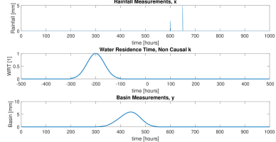
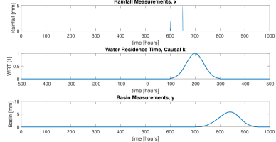
In Figure 1, we present the convolution of two rainfall Diracs with a residence time curve. We convolve the rainfall time series once with a residence time curve found in the negative time domain (causality is not respected) and once when this curve is in the positive time domain (causality is respected). The resulting breakthrough curve appears before the rain events in the first case which is wrong. In the second case the breakthrough curve appears after these rainfall events as expected for real applications. In the non-causal case lobes can appear in the negative time domain also, incorporating energy that should be present in the residence time curve thus reducing its amplitude and distorting its shape.

Figure 1: Enforcing causality while doing the convolution in the Fourier Domain needs to include the negative time domain interval of the residence time.

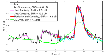
In Figure 2 we estimate with the AM algorithm all the possible residence time curves: with no positivity and no causality constraints applied, only the positivity constraint applied, only the causality constraint applied, and both positivity and causality constraints applied. In all cases, the convolution between the rainfall and these residence time curves give a reconstructed breakthrough curve that is similar in general shape with the real one. The best residence time estimation and breakthrough curve reconstruction are nonetheless the ones where both positivity and causality constraints are applied in the algorithm.

Figure 2: Different results for the $\textbf{k}_{est}$ for different constraints applied during the AM algorithm. All give a similar $\textbf{y}_{rec}$ but the best $\textbf{y}_{rec}$ and $\textbf{k}_{est}$ are those where both positivity and causality constraints are applied.

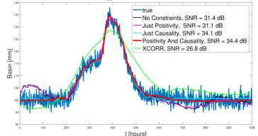
Furthermore, not applying the causality constraint all along the AM algorithm, and setting the negative time domain of $\textbf{k}_{est}$ to zero only at the end, would lead to a suboptimal solution caused by the way in which the AM algorithm navigates through the optimality map attached to the given functional: any change in the estimated vector $\textbf{k}_{est}$ at the end of the algorithm moves the value of the functional away from the optimal point that was estimated in the last iteration McCormick [1969], Bertsekas [1982].

5 Discussion on Related Work

Non-parametric deconvolution techniques with/without positivity constraints exist from the 1980s. How is our method different from those and why benchmarking it against the cross-correlation?

5.1 Comparison to Previous Works

As a first example, let’s take Neuman et al. [1982] which does a regularized non-parametric deconvolution and uses a bi-criterion curve; it navigates the optimality map to find the optimal estimation of the residence time by using a lag-one auto-correlation coefficient between the two error criteria. We consider this to be similar to our approach but our functional has a simpler, unified formulation from the direct model’s point of view and a different method to navigate the optimality map through the Projected Newton method in the AM algorithm. Also in the cited article there is no discussion about positivity, smoothness and causality of the estimated residence time.

In the case of the Skaggs et al. [1998] article, the direct model is similar to ours with some differences in its formulation:

$$(\hat{f},\hat{\alpha})=\underset{f\in\mathbbm{R}_{+}^{K},\alpha}{\text{argmin}}=\frac{1}{2}\|c-A\cdot f\|_{2}^{2}+\alpha^{2}\|\nabla^{2}f\|_{2}^{2}$$ (9)

$$\text{with }f\geq 0\ ,\ a^{\prime}f=1\ ,$$

where

• $c$ is the output of the system, known;

• $a$ is the input of the system, known;

• $A$ is the Toeplitz matrix of the input of the system;

• $f$ is the impulse response of the system, to estimate;

• $\alpha$ is the hyper-parameter to estimate with Fischer’s Statistic method;

• $\nabla^{2}f$ denotes the Hessian of $f$

The hyper-parameter $\alpha$ is here squared and determined with Fischer’s Statistic method ($F$), while smoothness is implemented by a second derivative applied on $f$. There is a constraint for positivity and the condition that the integral of the obtained curve sums up to 1. The solutions are evaluated with Provencher [1982] Fischer’s Statistic method and visual inspection. Another aspect here is the multiple peak problem, where Provencher [1982] argues to investigate separately for certain values of $F$. Also, to avoid computational difficulties in the test runs, a basis function representation of $f$ was introduced to ensure linearity between the probability density function (pdf) representation and the transport model. A causality constraint is not discussed here. In contrast, we estimate the $\alpha$ hyper-parameter ($\lambda$ in our case) by using the $SNR$ values between the reconstructed breakthrough curve and the original one. A bigger $SNR$ means a better reconstruction and also a better estimation of $k$ through the constraints, and this is realized through the $\lambda$ hyper-parameter possible choice strategies ($\alpha$ equivalent). A hydrologist can then estimate the same curve with a range of values for $\lambda$, for multiple time series and time series lengths, and then see what $\lambda$ value best fits for that particular tested site. We do smoothness regularization with a first-order derivative since testing with a second-order derivative does not show any improvement on the estimate, thus our direct model is slightly simpler. Our algorithm does not make an a priori assumption about the shape of the estimated residence time, therefore multiple lobes can appear without having to set any fixed number of these beforehand. The estimation of $f$ ($k$ in our case) is also free of being modeled with basis functions. The sole observation here is that the channel needs to be short enough so that it can be considered linear.

In the case of Fienen et al. [2006] the presented method is a Bayesian Monte-Carlo non-parametric deconvolution method that gives as result the full shape of the residence time distribution curve containing all possible residence time curves for that channel with zones of interest curves and the average curve. The method can yield multiple peaks in the transfer function with some computational cost – ”Using the MCMC Gibbs sampler with reflected Brownian motion requires some computational effort (CPU time up to several days on a typical desktop computer)” Fienen et al. [2006]. There is a constraint for positivity and for causality through Michalak & Kitanidis [2003]. Expectation Maximization is used to estimate the parameters. The algorithm is tested on uni-modal and bi-modal cases. In comparison, our method provides faster estimates of the residence time curve for a Dirac-like rainfall event or for a clustered rainfall event. The computational cost per tested hyper-parameter $\lambda$ is small. There is no constraint on the shape of the residence time curve other than smoothness (controlled by $\lambda$), and positivity and causality which we implement throughout the algorithm. On the downside, our algorithm does not estimate the uncertainties attached to the residence time like in a Bayesian approach.

Another example is Dietrich & Chapman [1993] with an algorithm based on ridge regression, where the direct model is similar to ours but has two hyper-parameters to be set. Michalak & Kitanidis [2003] is another article where Bayesian Monte-Carlo deconvolution is done through an inverse problem setup. Here positivity and causality are implicitly enforced by the method of images applied to reflected Brownian motion that gives ”a prior pdf that is non-zero only in the non-negative parameter range” Michalak & Kitanidis [2003]. The MCMC is here implemented with the Gibbs sampling algorithm. Similar to Fienen et al. [2006] the result is also a pdf with zones of interest for the residence time curve. Even if the computational time for Bayesian MCMC deconvolution methods is deemed ”manageable” Michalak & Kitanidis [2003], probably even more so with current hardware, the need for a fast method seems necessary for the community, and we expand on this in the next paragraph.

5.2 Comparison to the Cross-Correlation Method

We use the cross-correlation method as a benchmark to compare the performance of our algorithm. The cross-correlation measures the similarity between two signals, the second one being a shifted version of itself.

The AM algorithm also estimates the basin measurements constant level, $\textbf{c}_{est}$, and the estimated residence time amplitude depends on this constant level. It is necessary to obtain this same amplitude for the cross-correlation method, for comparison purposes, and this is done through the following:

$$\textbf{y}_{rec}=x\ast R_{xy}$$ (10)

$$\textbf{k}_{est}=R_{xy}\cdot\dfrac{\sigma_{\textbf{y}}}{\sigma_{\textbf{y}_{rec}}}$$

We call the cross-correlation method XCORR in our plots.

The cross-correlation implicitly assumes that the input rainfall is white noise. In this case, the auto-correlation of each rain fall time series would be a Dirac at the center. Since real rainfall time series have actually long-tailed statistics, the cross-correlation method is inexact. Here we use multifractals to simulate realistic rainfall Tessier et al. [1996]. Therefore, we expect the cross-correlation method to have a limited performance in real life tests.

The decision to benchmark against the cross-correlation is due to the fact that it is the preferred method for hydrologists in numerous recent articles: for determining transport of biological constituents in Sheets et al. [2002], or studying river-groundwater interaction with different types of measurements being cross-correlated like in Hoehn & Cirpka [2006]. Cross-correlation is also used by Vogt et al. [2010] for estimating mixing ratios and mean residence times, by Delbart et al. [2014] for estimating the pure residence time curve. Therefore, the hydrology community is interested in a simple and fast method with minimal implementation time that gives a residence time curve estimation from different time series measurements. In the case of the cross-correlation method, one focuses on analyzing the position of the maximal amplitude and general shape of the curve. From this curve hydrologists extract the characteristics of interest for that particular channel (mean residence time, mixing ratios, etc.). In contrast to the cross-correlation method we offer positivity, smoothness and causality constraints that give a more precise curve and a similar computing time.

5.3 Comparison to Cirpka et al. [2007]

Another benchmark method for the AM is the one presented in Cirpka et al. [2007] that uses measurements in fluctuations of electrical-conductivity as inputs, with a direct model similar to (1). The algorithm in Cirpka et al. [2007] is the same as the one used in Vogt et al. [2010] and both articles compare their results with those of the cross-correlation method. In Cirpka et al. [2007] the deconvolution algorithm is also an Alternating Minimization algorithm, but this time between estimating the residence time in the first step using a Bayesian Maximum A Posteriori method, and estimating the variance of the noise and the slope parameters in the second step. One can notice that Equation (3) is similar to [Cirpka et al., 2007, Eq.(8)]. One main advantage of the Cirpka et al. [2007] approach is that it delivers the uncertainty curves of the full Bayesian method while not being a full Bayesian deconvolution method, thus having a fast computation time. One drawback is that the two parameters, variance of noise and slope, need to have well chosen initial values. In a full Bayesian based deconvolution these parameters would also need to be estimated and this would be done by Markov Chain Monte Carlo methods which are computationally intensive. With regularization based deconvolution we try to avoid high computational costs and having multiple parameters that need carefully chosen initial values. The optimal value for our hyper-parameter $\lambda$ can be automatically obtained from the inputs.

6 Synthetic Data

6.1 General Discussion and $\lambda$ Choice Strategies

In the context of a realistic synthetic validation we generate the rain signals x with a multifractal simulation based on Tessier et al. [1996]. We use the multifractal parameters $H=-0.1,C1=0.4,\alpha=0.7$. Furthermore we simulate k with a Beta distribution $B(x,\alpha=2,\beta=6)$. We choose arbitrarily $c=100$. To evaluate the computed estimates we use the SNR definition, where we replace the noise term with the estimated $\textbf{k}_{est}$ signal or the $\textbf{y}_{rec}$ signal respectively.

$$SNR=20\log_{10}\dfrac{\|m\|_{2}^{2}}{\|m-m_{est}\|_{2}^{2}}[dB]\ ,$$ (11)

where $m$ is the true signal k or y and $m_{est}$ is the estimated $\textbf{k}_{est}$ or reconstructed $\textbf{y}_{rec}$ signal respectively.

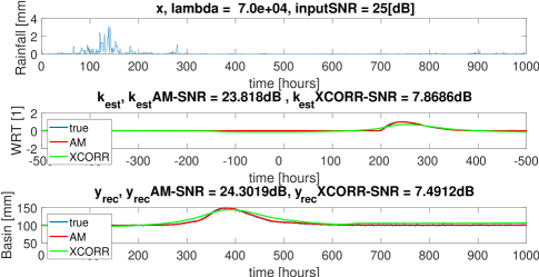
Examples of results obtained from synthetic data are shown in Figure 3 and Figure 4. The positivity and causality constraints are well respected. In addition, our method always provides a better estimation of the residence time $\textbf{k}_{est}$ in comparison with the standard cross-correlation method. The cross-correlation method manages to preserve the position of the maximum intensity of the residence time distribution but does not match either the shape or the amplitude of the true k. It can be observed that for a high noise level of y, the $\lambda$ hyper-parameter must be greater in order to obtain better estimates $\textbf{k}_{est}$ and $\textbf{y}_{rec}$. The greater the $\lambda$, the greater the importance of the regularization term in comparison to the fidelity term therefore smoothing is more important, which improves results when entries are noisy. Therefore, an analysis of the deconvolution results is also necessary in order to find the right adaptation of the $\lambda$ hyper-parameter for a particular noise level.

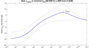
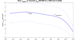
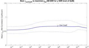
We propose four strategies to automatically tune the $\lambda$ hyper-parameter.

1. $\lambda_{oracle}$: choosing the $\lambda$ corresponding to the best estimation of $\textbf{k}_{est}$ by maximizing the $\textbf{k}_{est}$ SNR output (or minimizing the distance between $\textbf{k}_{est}$ and k). This strategy only works if the solution is known and represents the maximum achievable value.

2. $\lambda_{discrepancy}$: choosing the $\lambda$ giving the residual variance between y and $\textbf{y}_{rec}$ closest to that of the noise. This method is known as ”Morozov’s discrepancy principle”  Pereverzev & Schock [2009].

3. $\lambda_{fidelity}$: choosing the $\lambda$ corresponding to the best reconstruction of $\textbf{y}_{rec}$ by maximizing the $\textbf{y}_{rec}$ SNR output (or minimizing the distance between $\textbf{y}_{rec}$ and y). This is the value of the reconstruction optimum. This completely heuristic method automatically selects the hyper-parameter with a performance close to the selection by ”discrepancy principle” as will be seen next, in a completely blind way (without a priori knowledge of the variance of the noise).

4. $\lambda_{corrCoeff}$: choosing the $\lambda$ corresponding to the best reconstruction of $\textbf{y}_{rec}$ by maximizing the correlation coefficient value between $\textbf{y}_{rec}$ and y.

Figure 3: Two examples of the residence time estimation $\textbf{k}_{est}$ and reconstructed aquifer levels $\textbf{y}_{rec}$ from synthetic data for a y input SNR of 5 dB (noisy measurements). The input rain is generated with realistic multifractal time series. AM stands for the Alternating Minimization, XCORR for the standard cross-correlation, true for the true solution.

Figure 4: Same as in Figure  3 for a y input SNR of 25 dB.

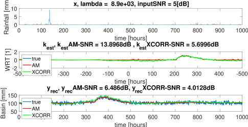
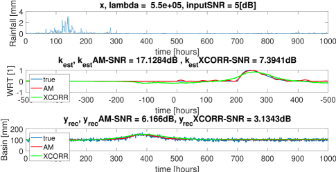
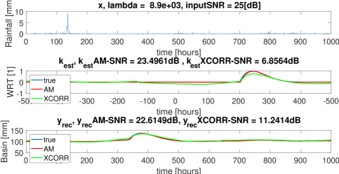
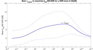
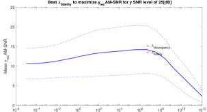
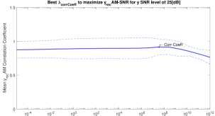
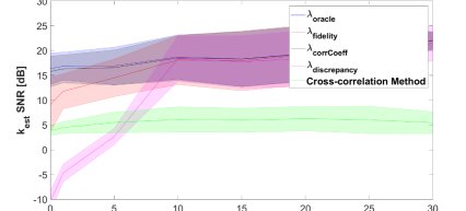
The four $\lambda$ strategies give different estimates of $\textbf{k}_{est}$, whose SNR value is compared to the y input SNR (measurements noise level), the goal being to obtain the best possible $\textbf{k}_{est}$ SNR for each given y input SNR level. The algorithm is tested for different input SNR values from 0 dB (very high noise level) to 30 dB (almost no noise) and over a $\lambda$ range chosen from $10^{-5}$ to $10^{12}$ with 20 values dispersed on a logarithmic scale.

To show the quality of estimation, for each noise level, we run arbitrarily 30 test cases (input rainfall x). For each randomly chosen x convolved with the known k, the resulting y signal has Gaussian noise added to it according to the input SNR test value. We apply the AM, XCORR and Cirpka et al. [2007] methods to each test case for all $\lambda$s. For each test run we record the $\textbf{k}_{est}$ SNR value, the $\textbf{y}_{rec}$ SNR value and the $\textbf{y}_{rec}$ correlation coefficient. Since 30 tests are made for each input y SNR, we obtain 30 plots showing the evolution of the $\textbf{k}_{est}$ SNR, of $\textbf{y}_{rec}$ SNR and $\textbf{y}_{rec}$ correlation coefficient, depending on the $\lambda$ choice.

By averaging these plots, mean values and their standard deviation can be computed which are shown in Figure 5 for a y input SNR of 5 dB and Figure 6 for 25 dB respectively. We lose the optimality for each single example due to averaging, but we show the variability of the criteria depending on noise level and input data. We also present graphically the four strategies of $\lambda$ determination.

Figure 5: Selection strategy of hyper-parameter $\lambda$. We plot average and standard deviation over 30 synthetic examples of: (a) $\textbf{k}_{est}$ SNR, (b) $\textbf{y}_{rec}$ SNR and (c) $\textbf{y}_{rec}$ correlation coefficient as a function of $\lambda$. The $y$ input SNR is 5 dB, meaning very noisy measurements. The $\lambda_{oracle}$ point in (a) shows the best $\lambda$ in average to maximize the $\textbf{k}_{est}$ SNR for the synthetic tests. This can be computed only when the true solution is known. In (b) the $\lambda_{fidelity}$ maximizes the $\textbf{y}_{rec}$ SNR. The $\lambda_{discrepancy}$ is achieved when $\textbf{y}_{rec}$ SNR is closest to the actual noise level. In (c), the $\lambda_{corrCoeff}$ is the optimum over the correlation coefficient between $\textbf{y}_{rec}$ and y.

Figure 6: Same as in Figure  5 with an y input SNR of 25 dB. We find that $\lambda_{fidelity}$, $\lambda_{discrepancy}$ and $\lambda_{corrCoeff}$ approach the optimal $\lambda_{oracle}$ in average.

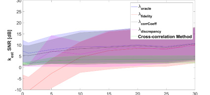
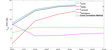
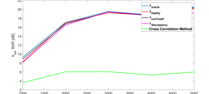
In Figure 7, we can see how the four strategies compare with the cross-correlation method. For a $\textbf{k}_{est}$ length of 1000 data points to estimate, we show in (a) the results for when inputs x and y are 1000 data points long and in (b) the results for when they are 5000 data points long. The $\textbf{k}_{est}SNR$ is always the best for the $\lambda_{oracle}$ strategy as expected. Across the plots, $\lambda_{corrCoeff}$ performs closest to it. The $\lambda_{fidelity}$ strategy is similar to $\lambda_{discrepancy}$ for SNRs from $10$ dB to $30$ dB. For the highest noise level, y input $SNR<$ 10 dB, $\lambda_{fidelity}$ is worst for short time series and $\lambda_{discrepancy}$ is worst for longer time series. Whatever the strategy, our method is always better than the cross-correlation.

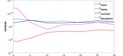
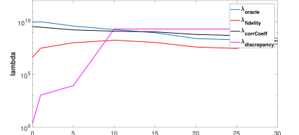
The average optimal $\lambda$ value for each strategy, given the y input SNR level, is presented in Figure 8. In (a) and (b), we see the evolution of the $\lambda$ values versus the y input SNR for the four given strategies. The four strategies of the hyper-parameters $\lambda$ are similar at low noise level, down to 10 dB for both 1000 and 5000 data points. Then, they begin to diverge but $\lambda_{corrCoeff}$ always stays in the neighborhood of $\lambda_{oracle}$, meaning it is a valid strategy to use in real test cases where k is not known. At very high noise levels for 1000 data points, $\lambda_{discrepancy}$ increases and provides an over-regularized, highly smooth solution that is far from the optimum. For 5000 data points both $\lambda_{fidelity}$ and $\lambda_{discrepancy}$ deliver smaller $\lambda$s. If for $\lambda_{fidelity}$ we can still expect that it would deliver a proper $\textbf{k}_{est}$, we can suspect that $\lambda_{discrepancy}$ would stress more an attachment to the data. This means that the estimated $\textbf{k}_{est}$ would give a $\textbf{y}_{rec}$ that would follow too closely the shape of $y$, including its noise.

Furthermore we investigate the influence of data volume on the k estimate. The aggregated results are presented in Figure 9, (a) for a y input SNR of 5 dB and in (b) for a y input SNR of 25 dB. All of our four strategies show significant improvement when the input time series of rainfall and aquifer measurements are longer, especially when the measurements are noisy.

Figure 7: Quality of the residence time estimation $\textbf{k}_{est}$ for the four hyper-parameter selection strategies and the cross-correlation method. Mean and standard deviation of obtained $\textbf{k}_{est}$ SNRs, as a function of the noise level of the measurements, for inputs of length: 1000 data points (a) and 5000 data points (b). The cross-correlation method always stands lower indicating a poorer estimation. The correlation coefficient strategy $\lambda_{corrCoeff}$ is the best strategy, across noise level and signal length.

Figure 8: The evolution of the four $\lambda$ strategies depending on the input SNR. For 1000 data points in (a) and 5000 data points in (b).

Figure 9: Quality of residence time $\textbf{k}_{est}$ estimation depending on the number of data points contained by x (input rain) and y (output aquifer level). We can observe that more data points lead to a better estimation for our method for all four $\lambda$ strategies. (a) is for a y input SNR of 5 dB and (b) is for a y input SNR of 25 dB

6.2 Comparison to Similar Methods

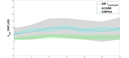
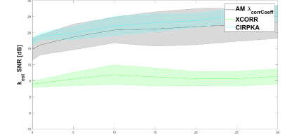
In Figure 10, we can see how our method compares to the cross-correlation method and the algorithm described in Cirpka et al. [2007] for various y input SNRs and 1000 and 5000 data points respectively (positive time interval of residence time to be estimated of 500 data points). Our method and the Cirpka et al. [2007] algorithm show similarly good results in comparison with the cross-correlation. The method of Cirpka et al. [2007] has a smaller standard deviation than our method, showing a weaker dependence of the noise/structure of the dataset.

Figure 10: Comparison between our algorithm, the cross-correlation and the Cirpka et al. [2007] algorithm for 1000 data points (a) and 5000 data points (b)

While our proposed approach provides different output results depending on the given $\lambda$, the best solution being picked automatically, the operator can choose an appropriate solution based on his own expertise, from an appropriate range around the optimal $\lambda$. Moreover, the solution is independent from the initialization due to the convexity of the $J$ functional.

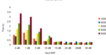
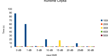
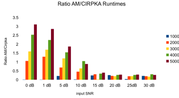
In Figure 11, bar plots illustrate the average runtime for 30 test cases, for different y input SNRs, for the three algorithms. The AM algorithm is consistently faster than the  Cirpka et al. [2007] algorithm for y input SNRs higher than 15 dB 11. It is also faster for the small data sets of 1000 points 11,11.

Figure 11: Analysis of runtimes between the AM algorithm and the Cirpka et al. [2007] algorithm for various lengths of the dataset and various noise levels.

7 Real Data

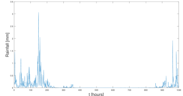
The tests on real data are conducted on data sets made available from the ”Base de Données des Observatoires en Hydrologie” $\copyright$ Irstea, Irstea [2017]. The data is gathered in the Ile de France region, in France. The measurements are from two neighboring sites, one at a higher altitude for rainfall measurements and the second at a lower altitude for aquifer measurements, taken at every 1 hour intervals, between January $1^{st}$, 2016 until January $1^{st}$, 2017.

For the real data, the estimates are based on the $\lambda_{corrCoeff}$ strategy with $\lambda$s chosen around the optimal values found with the synthetic data set, between $10^{8}$ to $10^{2}$. In Figure 12 and in Figure 13, estimates of the residence time for real life measurements of x and y are shown.

Figure 12: Examples of results for real data using the $\lambda_{corrCoeff}$ strategy. We estimate the residence time $\textbf{k}_{est}$ and the aquifer level $\textbf{c}_{est}$; we also plot the breakthrough curve $\textbf{y}_{rec}$ in blue. AM stands for the Alternating Minimization, XCORR for the standard cross-correlation, the true residence time k is not known. The position of the maximum amplitude of $\textbf{k}_{est}$ is similar for the two methods but the shape of $\textbf{k}_{est}$ varies significantly. Only the AM method has the physical properties of positivity and causality.

Figure 13: Same as in Figure 12.

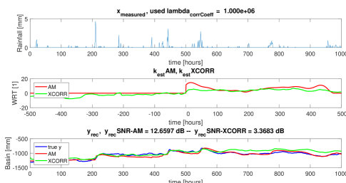
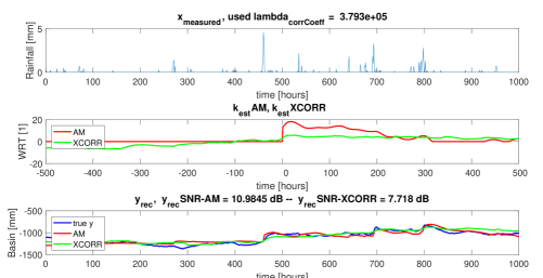
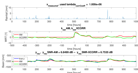
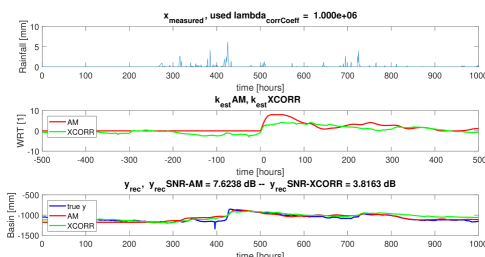
In all cases, the estimated curves honor the given positivity and causality constraints. For the cross-correlation, even if the $\textbf{y}_{rec}$ is close to the original y, the curve for the residence time estimated by this method has the disadvantage to not respect the positivity and causality constraints across all of the presented cases.

The aquifer level measurements have negative values due to the conventions of the used measuring instruments. The AM algorithm is also capable of estimating the aquifer average level c, and depending on this constant and the amplitude of the rain fall input, the estimated residence time curve $\textbf{k}_{est}$ will also have a certain amplitude (the curve is not normalized to resemble that of a pdf).

The AM algorithm succeeds in reconstructing the $\textbf{y}_{rec}$ with an SNR around 10 dB in the studied cases, using the $\lambda_{corrCoeff}$ and provides a better reconstruction SNR than the cross-correlation (XCORR) method.

We find small but significant changes in the residence time curve for different data sets of the same channel, as also identified in other datasets Delbart et al. [2014]. This may be due to the seasonal variability of the inputs (rainfall) and its effects on the hydrological process. This aspect would be of interest to study into more detail for specific sites to better understand it.

Another observation to be made is the fact that if non-linearities of the system are present (in transit or at the aquifer level), our approach may also lead to over simplification. Nonetheless the question arises if a hydrological channel could be considered as a linear and stationary system by parts (smaller time series) and therefore allow the use of our method for estimating partial residence time curves which can then be put together in a more complex mapping of the channel.

One can also note in the plots that the $\textbf{y}_{rec}$ is slightly better for cases when a heavy rainfall event appears at the beginning of the time series x instead of towards the end, suggesting the fact that the residence time estimation would also be better.

Finally, the examples show the appearance of multiple lobes that are considered a sign of reservoirs of the hydrological channel keeping part of the water for some time before releasing it in a later discharge. This demonstrates the usefulness of a non-parametric deconvolution method in comparison with parametric deconvolution methods where such lobes are either ignored or fixed in number.

8 Conclusion

We propose a new approach to estimate a smooth residence time taking into account positivity and causality constraints and having a fast runtime. We highlight why these constraints must be used all along the algorithmic process to reach the expected solution in the case of non-parametric 1D deconvolution for the AM algorithm presented here.

The estimation of the residence time $\textbf{k}_{est}$ was done using a fast Alternating Minimization algorithm with two steps: (1) 1D deconvolution and (2) estimation of the aquifer initial level. All tests have been done on a personal laptop, with CPU Intel(R) Core(TM) i7-6600U CPU @ 2.6GHz 2.81 GHz, 16.0 GB RAM, 64-bit OS, x-64-based processor, using Matlab^®. We validated the approach on synthetic tests and proposed several strategies to automatically estimate a hyper-parameter, $\lambda$, that controls the smoothness of the residence time curve. We have found that between these strategies, the correlation coefficient strategy seems to be very efficient to estimate the best value for $\lambda$.

We validated our AM method on synthetic data and found that the results are better than the standard cross-correlation method and similar to those of the Cirpka et al. [2007] method. We also demonstrated the capabilities of our AM method on real data. Additionally, our method respects the physical constraints (positivity, causality, non-circularity) which are important for interpretation purposes. The estimation made by our method will provide better information for hydro-geologists on amplitude and full shape of the residence time, the mean level of the aquifer and will also improve the estimation of the mean residence time (A shows how to compute it).

As possible improvements we propose refining this methodology for the potential non-linear aspects of the water transit time through the medium.

The Matlab implementation of the algorithm is available under CECILL license at the following public Git repository: https://git.l2s.centralesupelec.fr/meresescual/SmoothSignalEstimatorDeconvolution.git.

Appendix A Mean Residence Time

In order to estimate the mean residence time $\tau$, one has to simply renormalize the estimated transfer function $\textbf{k}_{est}$ and take the mean:

$$\tau=\sum_{t=0}^{t=\dfrac{K}{2}}\left(\dfrac{\textbf{k}_{est}(t)\cdot t}{\displaystyle\sum_{t=0}^{t=\dfrac{K}{2}}\textbf{k}_{est}(t)}\right)$$ (12)

References

- Bertsekas [1982] Bertsekas, D. P. (1982). Projected newton methods for optimization problems with simple constraints. SIAM Journal on control and Optimization, 20, 221–246. doi:https://doi.org/10.1137/0320018.
- Botter et al. [2011] Botter, G., Bertuzzo, E., & Rinaldo, A. (2011). Catchment residence and travel time distributions: The master equation. Geophysical Research Letters, 38, n/a–n/a. URL: http://dx.doi.org/10.1029/2011GL047666. doi:10.1029/2011GL047666. L11403.
- Cirpka et al. [2007] Cirpka, O. A., Fienen, M. N., Hofer, M., Hoehn, E., Tessarini, A., Kipfer, R., & Kitanidis, P. K. (2007). Analyzing bank filtration by deconvoluting time series of electric conductivity. Ground Water, 45, 318–328. URL: http://dx.doi.org/10.1111/j.1745-6584.2006.00293.x. doi:10.1111/j.1745-6584.2006.00293.x.
- Delbart et al. [2014] Delbart, C., Valdes, D., Barbecot, F., Tognelli, A., Richon, P., & Couchoux, L. (2014). Temporal variability of karst aquifer response time established by the sliding-windows cross-correlation method. Journal of Hydrology, 511, 580–588. doi:10.1016/j.jhydrol.2014.02.008.
- Dietrich & Chapman [1993] Dietrich, C., & Chapman, T. (1993). Unit graph estimation and stabilization using quadratic programming and difference norms. Water resources research, 29, 2629–2635.
- Dzikowski & Delay [1992] Dzikowski, M., & Delay, F. (1992). Simulation algorithm of time-dependent tracer test systems in hydrogeology. Computers & Geosciences, 18, 697 – 705. URL: http://www.sciencedirect.com/science/article/pii/009830049290004B. doi:http://dx.doi.org/10.1016/0098-3004(92)90004-B.
- Etcheverry & Perrochet [2000] Etcheverry, D., & Perrochet, P. (2000). Direct simulation of groundwater transit-time distributions using the reservoir theory. Hydrogeology Journal, 8, 200–208. URL: http://dx.doi.org/10.1007/s100400050006. doi:10.1007/s100400050006.
- Fienen et al. [2008] Fienen, M. N., Clemo, T., & Kitanidis, P. K. (2008). An interactive bayesian geostatistical inverse protocol for hydraulic tomography. Water Resources Research, 44.
- Fienen et al. [2006] Fienen, M. N., Luo, J., & Kitanidis, P. K. (2006). A bayesian geostatistical transfer function approach to tracer test analysis. Water Resources Research, 42.
- Gooseff et al. [2011] Gooseff, M. N., Benson, D. A., Briggs, M. A., Weaver, M., Wollheim, W., Peterson, B., & Hopkinson, C. S. (2011). Residence time distributions in surface transient storage zones in streams: Estimation via signal deconvolution. Water Resources Research, 47, n/a–n/a. URL: http://dx.doi.org/10.1029/2010WR009959. doi:10.1029/2010WR009959. W05509.
- Hoehn & Cirpka [2006] Hoehn, E., & Cirpka, O. A. (2006). Assessing residence times of hyporheic ground water in two alluvial flood plains of the southern alps using water temperature and tracers. Hydrology and Earth System Sciences, 10, 553–563. URL: https://www.hydrol-earth-syst-sci.net/10/553/2006/. doi:10.5194/hess-10-553-2006.
- Irstea [2017] Irstea (2017). ”base de données des observatoires en hydrologie” irstea. URL: https://bdoh.irstea.fr/ORACLE/.
- Long & Derickson [1999] Long, A., & Derickson, R. (1999). Linear systems analysis in a karst aquifer. Journal of Hydrology, 219, 206–217.
- Luo et al. [2006] Luo, J., Cirpka, O. A., Fienen, M. N., Wu, W.-m., Mehlhorn, T. L., Carley, J., Jardine, P. M., Criddle, C. S., & Kitanidis, P. K. (2006). A parametric transfer function methodology for analyzing reactive transport in nonuniform flow. Journal of contaminant hydrology, 83, 27–41.
- Massei et al. [2006] Massei, N., Dupont, J., Mahler, B., Laignel, B., Fournier, M., Valdes, D., & Ogier, S. (2006). Investigating transport properties and turbidity dynamics of a karst aquifer using correlation, spectral, and wavelet analyses. Journal of Hydrology, 329, 244 – 257. URL: http://www.sciencedirect.com/science/article/pii/S0022169406000965. doi:http://doi.org/10.1016/j.jhydrol.2006.02.021.
- McCormick [1969] McCormick, G. P. (1969). Anti-zig-zagging by bending. Management Science, (pp. 315–320).
- McGuire & McDonnell [2006] McGuire, K. J., & McDonnell, J. J. (2006). A review and evaluation of catchment transit time modeling. Journal of Hydrology, 330, 543–563. URL: http://dx.doi.org/10.1016/j.jhydrol.2006.04.020. doi:10.1016/j.jhydrol.2006.04.020.
- Michalak & Kitanidis [2003] Michalak, A. M., & Kitanidis, P. K. (2003). A method for enforcing parameter nonnegativity in bayesian inverse problems with an application to contaminant source identification. Water Resources Research, 39.
- Neuman & De Marsily [1976] Neuman, S. P., & De Marsily, G. (1976). Identification of linear systems response by parametric programing. Water Resources Research, 12, 253–262. URL: http://dx.doi.org/10.1029/WR012i002p00253. doi:10.1029/WR012i002p00253.
- Neuman et al. [1982] Neuman, S. P., Resnick, S. D., Reebles, R. W., & Dunbar, D. B. (1982). Developing a new deconvolution technique to model rainfall-runoff in arid environments. Water Resources Research Center, University of Arizona, . URL: http://hdl.handle.net/10150/305311.
- O’Sullivan [1998] O’Sullivan, J. A. (1998). Alternating minimization algorithms: From blahut-arimoto to expectation-maximization. Springer Science+Business Media New York, (pp. 173–192). doi:10.1007/978-1-4615-5121-8_13.
- Payn et al. [2008] Payn, R. A., Gooseff, M. N., Benson, D. A., Cirpka, O. A., Zarnetske, J. P., Bowden, W. B., McNamara, J. P., & Bradford, J. H. (2008). Comparison of instantaneous and constant-rate stream tracer experiments through non-parametric analysis of residence time distributions. Water Resources Research, 44, n/a–n/a. URL: http://dx.doi.org/10.1029/2007WR006274. doi:10.1029/2007WR006274. W06404.
- Pereverzev & Schock [2009] Pereverzev, S., & Schock, E. (2009). Morozov’s discrepancy principle for tikhonov regularization of severely ill-posed problems in finite-dimensional subspaces. Numerical Functional Analysis and Optimization, . doi:http://dx.doi.org/10.1080/01630560008816993.
- Provencher [1982] Provencher, S. W. (1982). Contin: a general purpose constrained regularization program for inverting noisy linear algebraic and integral equations. Computer Physics Communications, 27, 229–242.
- Robinson et al. [2010] Robinson, B. A., Dash, Z. V., & Srinivasan, G. (2010). A particle tracking transport method for the simulation of resident and flux-averaged concentration of solute plumes in groundwater models. Computational Geosciences, 14, 779–792. URL: http://dx.doi.org/10.1007/s10596-010-9190-6. doi:10.1007/s10596-010-9190-6.
- Sheets et al. [2002] Sheets, R., Darner, R., & Whitteberry, B. (2002). Lag times of bank filtration at a well field, cincinnati, ohio, usa. Journal of Hydrology, 266, 162 – 174. URL: http://www.sciencedirect.com/science/article/pii/S0022169402001646. doi:https://doi.org/10.1016/S0022-1694(02)00164-6. Attenuation of Groundwater Pollution by Bank Filtration.
- Skaggs et al. [1998] Skaggs, T. H., Kabala, Z., & Jury, W. A. (1998). Deconvolution of a nonparametric transfer function for solute transport in soils. Journal of Hydrology, 207, 170–178.
- Tessier et al. [1996] Tessier, Y., Lovejoy, S., Hubert, P., Schertzer, D., & Pecknold, S. (1996). Multifractal analysis and modeling of rainfall and river flows and scaling, causal transfer functions. Journal of Geophysical Research: Atmospheres, 101, 26427–26440. URL: http://dx.doi.org/10.1029/96JD01799. doi:10.1029/96JD01799.
- Vogt et al. [2010] Vogt, T., Hoehn, E., Schneider, P., Freund, A., Schirmer, M., & Cirpka, O. A. (2010). Fluctuations of electrical conductivity as a natural tracer for bank filtration in a losing stream. Advances in Water Resources, 33, 1296–1308.
- Werner & Kadlec [2000] Werner, T. M., & Kadlec, R. H. (2000). Wetland residence time distribution modeling. Ecological Engineering, 15, 77–90. URL: http://dx.doi.org/10.1016/S0925-8574(99)00036-1. doi:10.1016/s0925-8574(99)00036-1.
- Zuo & Hu [2012] Zuo, B., & Hu, X. (2012). Geophysical model enhancement technique based on blind deconvolution. Computers & Geosciences, 49, 170 – 181. URL: http://www.sciencedirect.com/science/article/pii/S0098300412002129. doi:http://doi.org/10.1016/j.cageo.2012.06.017.