Hybrid Contact Preintegration for Visual-Inertial-Contact State Estimation Using Factor Graphs

Ross Hartley, Maani Ghaffari Jadidi, Lu Gan, Jiunn-Kai Huang, Jessy W. Grizzle, and Ryan M. Eustice The authors are with the College of Engineering, University of Michigan, Ann Arbor, MI 48109 USA {rosshart, maanigj, ganlu, bjhuang, grizzle, eustice}@umich.edu.
Abstract

The factor graph framework is a convenient modeling technique for robotic state estimation where states are represented as nodes, and measurements are modeled as factors. When designing a sensor fusion framework for legged robots, one often has access to visual, inertial, joint encoder, and contact sensors. While visual-inertial odometry has been studied extensively in this framework, the addition of a preintegrated contact factor for legged robots has been only recently proposed. This allowed for integration of encoder and contact measurements into existing factor graphs, however, new nodes had to be added to the graph every time contact was made or broken. In this work, to cope with the problem of switching contact frames, we propose a hybrid contact preintegration theory that allows contact information to be integrated through an arbitrary number of contact switches. The proposed hybrid modeling approach reduces the number of required variables in the nonlinear optimization problem by only requiring new states to be added alongside camera or selected keyframes. This method is evaluated using real experimental data collected from a Cassie-series robot where the trajectory of the robot produced by a motion capture system is used as a proxy for ground truth. The evaluation shows that inclusion of the proposed preintegrated hybrid contact factor alongside visual-inertial navigation systems improves estimation accuracy as well as robustness to vision failure, while its generalization makes it more accessible for legged platforms.

I Introduction and Related Work

Long-term state estimation and mapping for legged robots requires a flexible sensor fusion framework that allows for reducing drift and correcting past estimates as the robot perceives new information. During long-term missions, odometry systems can drift substantially since the absolute position and yaw (rotation about gravity) are unobservable [1, 2], leading to an unbounded growth in the covariance of the estimate and an undesirable expansion of the search space for data association tasks. The factor graph smoothing framework [3, 4, 5, 6] offers suitable machineries for building such systems in which real-time performance is achieved by exploiting the sparse structure of the Simultaneous Localization and Mapping (SLAM) problem [7, 8]. In addition, the incorporation of loop-closures [8] into the graph, upon availability, is convenient.

Legged robot perception often involves fusing kinematic odometry, Inertial Measurement Unit (IMU) data, and visual/depth measurements to infer the robot’s trajectory, controller inputs such as velocity, and calibration parameters [9, 10, 11, 12]. The challenge in such perception problems is the rigorous real-time performance requirements in legged robots arising from their direct and switching contact with the environment [1, 13, 14, 15, 16]. Furthermore, kinematic leg odometry involves estimating relative transformations and velocity using kinematic and contact information, which can be noisy due to the encoder noise and foot slip [17, 2].
Refer to caption
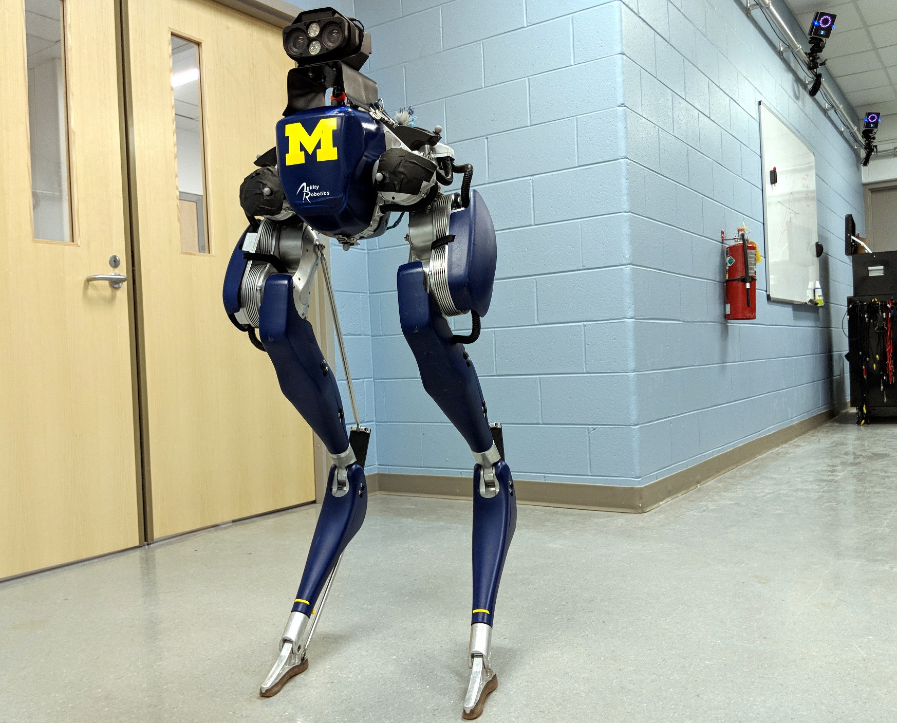
Figure 1: Experiments were conducted on a Cassie-series robot designed by Agility Robotics in an indoor laboratory environment. The motion capture system is used to record the robot trajectory as a proxy for ground truth data. The Cassie-series robot has 20 degrees of freedom, 10 actuators, joint encoders, an IMU, and mounted with a Multisense S7 stereo camera.

In our previous work [18], we made progress towards a long-term, legged robot state estimator by developing two novel factors that integrate the use of forward kinematics and the notion of contact between the robot and the environment into the factor graph framework. While these novel factors improved the estimator’s performance, new challenges emerged due to frequent switching contacts as the robot navigates through an environment. In particular, a new node needs to be added to the graph every time contact was made or broken. This leads to an larger number of optimization variables, which increases the complexity of the graph and ultimately slows down the estimator. This problem is only exacerbated as the number of contact points increases (quadraped or hexapod robots).

In this paper, we generalize the idea of the preintegrated contact factor in [18] to a hybrid preintegrated contact factor that alleviates the effect of frequently changing contacts with the environment. We develop a novel method for preintegrating contact information though an arbitrary number of contact switches. The proposed hybrid modeling approach reduces the number of required variables in the nonlinear optimization problem by only requiring new states to be added alongside camera or selected keyframes. The present work has the following contributions:

  1. i.

    A generic forward kinematic factor modeled in SE(3)SE3\mathrm{SE}(3) using the manipulator Jacobian that supports both prismatic and revolute joints; the factor incorporates noisy encoder measurements to estimate an end-effector pose at any time-step.

  2. ii.

    A hybrid preintegrated contact factor modeled in SE(3)SE3\mathrm{SE}(3) that allows for an arbitrary number of contact switches between camera or selected keyframes.

  3. iii.

    Real-time implementation and experimental evaluation of the derived factors on a Cassie-series biped robot in an indoor laboratory environment where ground truth data was collected using a motion capture system.

The remainder of this paper is organized as follows. Section II provides the mathematical background and preliminaries. We formulate the problem using the factor graph approach in Section III. Section IV explains the forward kinematic modeling and derives the forward kinematic factor. The proposed hybrid rigid contact model and hybrid contact preintegration are derived in Section V. Experimental evaluations of the proposed methods on a 3D biped robot (shown in Fig. 1) are presented in Section VI. Finally, Section VII concludes the paper and provides future work suggestions.

II Mathematical Background and Preliminaries

We first review the Lie group theory corresponding to the rotation and motion groups [19, 20]. Afterwards, we discuss the optimization technique on matrix Lie groups [21] and the choice of retraction for deriving forward kinematic and hybrid preintegrated contact factors.

Matrices are capitalized in bold, such as in X, and vectors are column-wise in lower case bold type, such as in x. We denote e𝐦𝐢𝐬𝐬𝐢𝐧𝐠𝚺2e𝖳𝚺1esuperscriptsubscriptdelimited-∥∥e𝐦𝐢𝐬𝐬𝐢𝐧𝐠𝚺2superscripte𝖳superscript𝚺1e\lVert\boldsymbol{\textbf{e}missing}\rVert_{\boldsymbol{\Sigma}}^{2}\triangleq\textbf{e}^{\mathsf{T}}\boldsymbol{\Sigma}^{-1}\textbf{e}. The n𝑛n-by-n𝑛n identity matrix and the n𝑛n-by-m𝑚m matrix of zeros are denoted by InsubscriptI𝑛\textbf{I}_{n} and 0n×msubscript0𝑛𝑚\textbf{0}_{n\times m} respectively. The vector constructed by stacking xisubscript𝑥𝑖x_{i}, i{1,,n}for-all𝑖1𝑛\forall\ i\in\{1,\dots,n\} is denoted by vec(x1,,xn)vecsubscript𝑥1subscript𝑥𝑛\mathrm{vec}(x_{1},\dots,x_{n}). The covariance of a random vector is denoted by 𝐂𝐨𝐯[]𝐂𝐨𝐯delimited-[]\mathbf{Cov}[\cdot]. Finally, we denote the base (IMU) frame of the robot by B, the world frame by W, and contact frame by C.

II-A Matrix Lie Group of Rotation and Motion in 3superscript3\mathbb{R}^{3}

The general linear group of degree n𝑛n, denoted by GLn()subscriptGL𝑛\mathrm{GL}_{n}(\mathbb{R}), is the set of all n×n𝑛𝑛n\times n nonsingular real matrices, where the group binary operation is the ordinary matrix multiplication. The three-dimensional (3D) special orthogonal group, denoted by SO(3)={RGL3()|RR𝖳=𝐈3,detR=+1}SO3conditional-setRsubscriptGL3formulae-sequencesuperscriptRR𝖳subscript𝐈3detR1\mathrm{SO}(3)=\{\textbf{R}\in\mathrm{GL}_{3}(\mathbb{R})\ |\ \textbf{R}\textbf{R}^{\mathsf{T}}=\mathbf{I}_{3},\operatorname{det}\textbf{R}=+1\} is the rotation group on 3superscript3\mathbb{R}^{3}. The 3D special Euclidean group, denoted by

SE(3)={H𝐦𝐢𝐬𝐬𝐢𝐧𝐠=[Rp01×31]GL4()|RSO(3),p3}SE3conditional-setsubscriptHsubscript𝐦𝐢𝐬𝐬𝐢𝐧𝐠matrixRpsubscript0131subscriptGL4formulae-sequenceRSO3psuperscript3\small\mathrm{SE}(3)=\{{}_{\text{}}\boldsymbol{\textbf{H}missing}_{\text{}}=\begin{bmatrix}\textbf{R}&\textbf{p}\\ \textbf{0}_{1\times 3}&1\end{bmatrix}\in\mathrm{GL}_{4}(\mathbb{R})\ |\ \textbf{R}\in\mathrm{SO}(3),\textbf{p}\in\mathbb{R}^{3}\}

is the group of rigid transformations on 3superscript3\mathbb{R}^{3}. The Lie algebra (tangent space at the identity together with Lie bracket) of SO(3)SO3\mathrm{SO}(3), denoted by 𝔰𝔬(3)𝔰𝔬3\mathfrak{so}(3), is the set of 3×3333\times 3 skew-symmetric matrices such that for any 𝝎vec(ω1,ω2,ω3)3subscriptsubscript𝝎vecsubscript𝜔1subscript𝜔2subscript𝜔3superscript3{}_{\text{}}\boldsymbol{\omega}_{\text{}}\triangleq\mathrm{vec}(\omega_{1},\omega_{2},\omega_{3})\in\mathbb{R}^{3}:

𝝎[0ω3ω2ω30ω1ω2ω10],superscript𝝎matrix0subscript𝜔3subscript𝜔2subscript𝜔30subscript𝜔1subscript𝜔2subscript𝜔10\small\boldsymbol{\omega}^{\wedge}\triangleq\begin{bmatrix}0&-\omega_{3}&\omega_{2}\\ \omega_{3}&0&-\omega_{1}\\ -\omega_{2}&\omega_{1}&0\\ \end{bmatrix},

and (𝝎)=𝝎superscriptsubscriptsuperscriptsubscript𝝎subscriptsubscript𝝎{({{}_{\text{}}\boldsymbol{\omega}_{\text{}}}^{\wedge})}^{\vee}={}_{\text{}}\boldsymbol{\omega}_{\text{}}. The Lie algebra of SE(3)SE3\mathrm{SE}(3), denoted by 𝔰𝔢(3)𝔰𝔢3\mathfrak{se}(3), can be identified by 4×4444\times 4 matrices such that for any 𝝎,v3subscriptsubscript𝝎vsuperscript3{}_{\text{}}\boldsymbol{\omega}_{\text{}},\textbf{v}\in\mathbb{R}^{3} and the twist is defined as 𝝃vec(𝝎,v)6𝝃vecsubscriptsubscript𝝎vsuperscript6\boldsymbol{\xi}\triangleq\mathrm{vec}({}_{\text{}}\boldsymbol{\omega}_{\text{}},\textbf{v})\in\mathbb{R}^{6}:

𝝃[𝝎v01×30]superscript𝝃matrixsubscriptsuperscriptsubscript𝝎vsubscript0130\boldsymbol{\xi}^{\wedge}\triangleq\begin{bmatrix}{}_{\text{}}\boldsymbol{\omega}_{\text{}}^{\wedge}&\textbf{v}\\ \textbf{0}_{1\times 3}&0\\ \end{bmatrix} (1)

where the wedge operator () for twist is overloaded.

The exponential map exp:𝔰𝔢(3)SE(3):𝔰𝔢3SE3\exp:\mathfrak{se}(3)\to\mathrm{SE}(3) can be used to map a member of 𝔰𝔢(3)𝔰𝔢3\mathfrak{se}(3) around a neighborhood of zero to a member of SE(3)SE3\mathrm{SE}(3) around a neighborhood of the identity. The logarithm map is the inverse, i.e., log:SE(3)𝔰𝔢(3):SE3𝔰𝔢3\log:\mathrm{SE}(3)\to\mathfrak{se}(3), and exp(log(H𝐦𝐢𝐬𝐬𝐢𝐧𝐠))=H𝐦𝐢𝐬𝐬𝐢𝐧𝐠subscriptHsubscript𝐦𝐢𝐬𝐬𝐢𝐧𝐠subscriptHsubscript𝐦𝐢𝐬𝐬𝐢𝐧𝐠\exp(\log({}_{\text{}}\boldsymbol{\textbf{H}missing}_{\text{}}))={}_{\text{}}\boldsymbol{\textbf{H}missing}_{\text{}}, H𝐦𝐢𝐬𝐬𝐢𝐧𝐠SE(3)subscriptHsubscript𝐦𝐢𝐬𝐬𝐢𝐧𝐠SE3{}_{\text{}}\boldsymbol{\textbf{H}missing}_{\text{}}\in\mathrm{SE}(3). Now we can define the difference between a transformation H𝐦𝐢𝐬𝐬𝐢𝐧𝐠SE(3)subscriptHsubscript𝐦𝐢𝐬𝐬𝐢𝐧𝐠SE3{}_{\text{}}\boldsymbol{\textbf{H}missing}_{\text{}}\in\mathrm{SE}(3) and its estimate with a small perturbation H𝐦𝐢𝐬𝐬𝐢𝐧𝐠~SE(3)~subscriptHsubscript𝐦𝐢𝐬𝐬𝐢𝐧𝐠SE3\tilde{{}_{\text{}}\boldsymbol{\textbf{H}missing}_{\text{}}}\in\mathrm{SE}(3) as [20, 22]:

ϵ=log(H𝐦𝐢𝐬𝐬𝐢𝐧𝐠1H𝐦𝐢𝐬𝐬𝐢𝐧𝐠~),superscriptbold-italic-ϵsubscriptHsuperscriptsubscript𝐦𝐢𝐬𝐬𝐢𝐧𝐠1~subscriptHsubscript𝐦𝐢𝐬𝐬𝐢𝐧𝐠\boldsymbol{\epsilon}^{\wedge}=\log({}_{\text{}}\boldsymbol{\textbf{H}missing}_{\text{}}^{-1}\tilde{{}_{\text{}}\boldsymbol{\textbf{H}missing}_{\text{}}}),

where ϵ𝔰𝔢(3)superscriptbold-italic-ϵ𝔰𝔢3\boldsymbol{\epsilon}^{\wedge}\in\mathfrak{se}(3). To define the norm and covariance of the error term, we exploit the fact that 𝔰𝔢(3)𝔰𝔢3\mathfrak{se}(3) is isomorphic to 6superscript6\mathbb{R}^{6}, i.e., ϵϵ6maps-tosuperscriptbold-italic-ϵbold-italic-ϵsuperscript6\boldsymbol{\epsilon}^{\wedge}\mapsto\boldsymbol{\epsilon}\in\mathbb{R}^{6} using the \vee operator. Therefore, we can define the 6×6666\times 6 covariance matrix conveniently as 𝚺ϵ=𝐂𝐨𝐯[ϵ]subscript𝚺bold-italic-ϵ𝐂𝐨𝐯delimited-[]bold-italic-ϵ\boldsymbol{\Sigma}_{\boldsymbol{\epsilon}}=\mathbf{Cov}[\boldsymbol{\epsilon}]. We use the following adopted simplified notations from [6]:

Exp:6𝝃exp(𝝃)SE(3)Log:SE(3)H𝐦𝐢𝐬𝐬𝐢𝐧𝐠log(H𝐦𝐢𝐬𝐬𝐢𝐧𝐠)6.\small{\begin{array}[]{llll}\mathrm{Exp}:\mathbb{R}^{6}&\ni\boldsymbol{\xi}&\rightarrow\exp(\boldsymbol{\xi}^{\wedge})&\in\mathrm{SE}(3)\\ \mathrm{Log}:\mathrm{SE}(3)&\ni{}_{\text{}}\boldsymbol{\textbf{H}missing}_{\text{}}&\rightarrow\log({}_{\text{}}\boldsymbol{\textbf{H}missing}_{\text{}})^{\vee}&\in\mathbb{R}^{6}.\end{array}}

The adjoint representation of a Lie group is a linear map that captures the non-commutative structure of the group. For SE(3)SE3\mathrm{SE}(3), the matrix representation of the adjoint map [20] is

AdH𝐦𝐢𝐬𝐬𝐢𝐧𝐠=[R03×3pRR].subscriptAdsubscriptHsubscript𝐦𝐢𝐬𝐬𝐢𝐧𝐠matrixRsubscript033superscriptpRR\mathrm{Ad}_{{}_{\text{}}\boldsymbol{\textbf{H}missing}_{\text{}}}=\begin{bmatrix}\textbf{R}&\textbf{0}_{3\times 3}\\ \textbf{p}^{\wedge}\textbf{R}&\textbf{R}\\ \end{bmatrix}. (2)

For any H𝐦𝐢𝐬𝐬𝐢𝐧𝐠SE(3)subscriptHsubscript𝐦𝐢𝐬𝐬𝐢𝐧𝐠SE3{}_{\text{}}\boldsymbol{\textbf{H}missing}_{\text{}}\in\mathrm{SE}(3) and 𝝃6𝝃superscript6\boldsymbol{\xi}\in\mathbb{R}^{6}, the adjoint map asserts

(AdH𝐦𝐢𝐬𝐬𝐢𝐧𝐠𝝃)=H𝐦𝐢𝐬𝐬𝐢𝐧𝐠𝝃H𝐦𝐢𝐬𝐬𝐢𝐧𝐠1Exp(AdH𝐦𝐢𝐬𝐬𝐢𝐧𝐠𝝃)=H𝐦𝐢𝐬𝐬𝐢𝐧𝐠Exp(𝝃)H𝐦𝐢𝐬𝐬𝐢𝐧𝐠1.superscriptsubscriptAdsubscriptHsubscript𝐦𝐢𝐬𝐬𝐢𝐧𝐠𝝃subscriptHsubscript𝐦𝐢𝐬𝐬𝐢𝐧𝐠superscript𝝃subscriptHsuperscriptsubscript𝐦𝐢𝐬𝐬𝐢𝐧𝐠1ExpsubscriptAdsubscriptHsubscript𝐦𝐢𝐬𝐬𝐢𝐧𝐠𝝃subscriptHsubscript𝐦𝐢𝐬𝐬𝐢𝐧𝐠Exp𝝃subscriptHsuperscriptsubscript𝐦𝐢𝐬𝐬𝐢𝐧𝐠1\small(\mathrm{Ad}_{{}_{\text{}}\boldsymbol{\textbf{H}missing}_{\text{}}}\boldsymbol{\xi})^{\wedge}={}_{\text{}}\boldsymbol{\textbf{H}missing}_{\text{}}\boldsymbol{\xi}^{\wedge}{}_{\text{}}\boldsymbol{\textbf{H}missing}_{\text{}}^{-1}\Rightarrow\mathrm{Exp}(\mathrm{Ad}_{{}_{\text{}}\boldsymbol{\textbf{H}missing}_{\text{}}}\boldsymbol{\xi})={}_{\text{}}\boldsymbol{\textbf{H}missing}_{\text{}}\mathrm{Exp}(\boldsymbol{\xi}){}_{\text{}}\boldsymbol{\textbf{H}missing}_{\text{}}^{-1}.

II-B Retraction Map and Optimization on Manifold

Given a retraction mapping and the associated manifold, we can optimize over the manifold by iteratively lifting the cost function of our optimization problem to the tangent space, solving the re-parameterized problem, and then mapping the updated solution back to the manifold using the retraction [21]. For SE(3)SE3\mathrm{SE}(3) we use its exponential map as the natural retraction, H𝐦𝐢𝐬𝐬𝐢𝐧𝐠(δ𝝃)=H𝐦𝐢𝐬𝐬𝐢𝐧𝐠Exp(δ𝝃)subscriptsubscriptHsubscript𝐦𝐢𝐬𝐬𝐢𝐧𝐠𝛿𝝃subscriptHsubscript𝐦𝐢𝐬𝐬𝐢𝐧𝐠Exp𝛿𝝃\mathcal{R}_{{}_{\text{}}\boldsymbol{\textbf{H}missing}_{\text{}}}(\delta\boldsymbol{\xi})={}_{\text{}}\boldsymbol{\textbf{H}missing}_{\text{}}\mathrm{Exp}(\delta\boldsymbol{\xi}), where δ𝝃6𝛿𝝃superscript6\delta\boldsymbol{\xi}\in\mathbb{R}^{6} is the twist defined earlier in (1). Therefore, the retractions on the base and the contact poses are defined as

XiXiExp(δxi)andCiCiExp(δci).subscriptX𝑖subscriptX𝑖Exp𝛿subscriptx𝑖andsubscriptC𝑖subscriptC𝑖Exp𝛿subscriptc𝑖\small\begin{split}\textbf{X}_{i}&\leftarrow\textbf{X}_{i}\mathrm{Exp}(\delta\textbf{x}_{i})\\ \end{split}\quad\text{and}\quad\begin{split}\textbf{C}_{i}&\leftarrow\textbf{C}_{i}\mathrm{Exp}(\delta\textbf{c}_{i}).\\ \end{split} (3)

These retractions are used to both update the state during optimization and to compute the Jacobians of the residuals.

III Problem Statement and Formulation

In this section, we formulate the state estimation problem using the factor graph framework where independent sensor measurements can be incorporated by introducing additional factors based on the associated measurement models. The biped robot, shown in Figure 1, is equipped with a stereo camera, an IMU mounted on the torso, joint encoders, and a series of springs used for binary contact detection. Without loss of generality, we assume the IMU and camera are collocated with the base frame of the robot.

III-A State Representation

The state variables (at time tisubscript𝑡𝑖t_{i}) include the 3D body pose, H𝐦𝐢𝐬𝐬𝐢𝐧𝐠WB(t)SE(3)subscriptHsubscript𝐦𝐢𝐬𝐬𝐢𝐧𝐠WB𝑡SE3{}_{\text{}}\boldsymbol{\textbf{H}missing}_{\text{WB}}(t)\in\mathrm{SE}(3), and velocity, vWBW(t)3subscriptsubscriptvWBW𝑡superscript3{}_{\text{W}}\textbf{v}_{\text{WB}}(t)\in\mathbb{R}^{3}, in the world frame, the 3D contact pose in the world frame, H𝐦𝐢𝐬𝐬𝐢𝐧𝐠WC(t)SE(3)subscriptHsubscript𝐦𝐢𝐬𝐬𝐢𝐧𝐠WC𝑡SE3{}_{\text{}}\boldsymbol{\textbf{H}missing}_{\text{WC}}(t)\in\mathrm{SE}(3), and the IMU bias, b(t)vec(bg(t),ba(t))6b𝑡vecsuperscriptb𝑔𝑡superscriptb𝑎𝑡superscript6\textbf{b}(t)\triangleq\mathrm{vec}\left(\textbf{b}^{g}(t),\textbf{b}^{a}(t)\right)\in\mathbb{R}^{6}, where bg(t)3superscriptb𝑔𝑡superscript3\textbf{b}^{g}(t)\in\mathbb{R}^{3} and ba(t)3superscriptb𝑎𝑡superscript3\textbf{b}^{a}(t)\in\mathbb{R}^{3} are the gyroscope and accelerometer biases, respectively. All together, the state at any time-step i𝑖i is a tuple as follows:

𝒯i(H𝐦𝐢𝐬𝐬𝐢𝐧𝐠WB(t),vWBW(t),H𝐦𝐢𝐬𝐬𝐢𝐧𝐠WC(t),b(t))(Xi,vi,Ci,bi)subscript𝒯𝑖subscriptHsubscript𝐦𝐢𝐬𝐬𝐢𝐧𝐠WB𝑡subscriptsubscriptvWBW𝑡subscriptHsubscript𝐦𝐢𝐬𝐬𝐢𝐧𝐠WC𝑡b𝑡subscriptX𝑖subscriptv𝑖subscriptC𝑖subscriptb𝑖\mathcal{T}_{i}\triangleq\left({}_{\text{}}\boldsymbol{\textbf{H}missing}_{\text{WB}}(t),{}_{\text{W}}\textbf{v}_{\text{WB}}(t),{}_{\text{}}\boldsymbol{\textbf{H}missing}_{\text{WC}}(t),\textbf{b}(t)\right)\triangleq\left(\textbf{X}_{i},\textbf{v}_{i},\textbf{C}_{i},\textbf{b}_{i}\right)

(4)

Further, it is convenient to denote the trajectory of the state variables up to time-step k𝑘k by 𝒳ki=1k𝒯isubscript𝒳𝑘superscriptsubscript𝑖1𝑘subscript𝒯𝑖\mathcal{X}_{k}\triangleq\bigcup_{i=1}^{k}\mathcal{T}_{i}. Foot slip is the major source of drift in kinematic leg odometry. The inclusion of the contact pose in the state tuple allows for isolating the noise at the contact point.

III-B Factor Graph Formulation

Let ijSE(3)subscript𝑖𝑗SE3\mathcal{L}_{ij}\in\mathrm{SE}(3) be a perceptual loop-closure measurement relating poses at time-steps i𝑖i and j𝑗j (j>i𝑗𝑖j>i) computed from an independent sensor, e.g. using a point cloud matching algorithm. The forward kinematic measurements at time-step i𝑖i are denoted by isubscript𝑖\mathcal{F}_{i}. The IMU and contact sensors provide measurements at higher frequencies. Between any two time-steps i𝑖i and j𝑗j, we denote the set of all IMU and contact measurements by ijsubscript𝑖𝑗\mathcal{I}_{ij} and 𝒞ijsubscript𝒞𝑖𝑗\mathcal{C}_{ij}, respectively. Let 𝒦ksubscript𝒦𝑘\mathcal{K}_{k} be the index set of time-steps (or keyframes) up to time-step k𝑘k. We denote the set of all measurements up to time-step k𝑘k by 𝒵k{ij,ij,i,𝒞ij}i,j𝒦ksubscript𝒵𝑘subscriptsubscript𝑖𝑗subscript𝑖𝑗subscript𝑖subscript𝒞𝑖𝑗𝑖𝑗subscript𝒦𝑘\mathcal{Z}_{k}\triangleq\{\mathcal{L}_{ij},\mathcal{I}_{ij},\mathcal{F}_{i},\mathcal{C}_{ij}\}_{i,j\in\mathcal{K}_{k}}.

By assuming the measurements are conditionally independent and are corrupted by additive zero mean white Gaussian noise, the posterior probability of the full SLAM problem can be written as p(𝒳k|𝒵k)p(𝒳0)p(𝒵k|𝒳k)proportional-to𝑝conditionalsubscript𝒳𝑘subscript𝒵𝑘𝑝subscript𝒳0𝑝conditionalsubscript𝒵𝑘subscript𝒳𝑘p(\mathcal{X}_{k}|\mathcal{Z}_{k})\propto p(\mathcal{X}_{0})p(\mathcal{Z}_{k}|\mathcal{X}_{k}), where

p(𝒵k|𝒳k)=i,j𝒦kp(ij|𝒳j)p(ij|𝒳j)p(i|𝒳i)p(𝒞ij|𝒳j).𝑝conditionalsubscript𝒵𝑘subscript𝒳𝑘subscriptproduct𝑖𝑗subscript𝒦𝑘𝑝conditionalsubscript𝑖𝑗subscript𝒳𝑗𝑝conditionalsubscript𝑖𝑗subscript𝒳𝑗𝑝conditionalsubscript𝑖subscript𝒳𝑖𝑝conditionalsubscript𝒞𝑖𝑗subscript𝒳𝑗p(\mathcal{Z}_{k}|\mathcal{X}_{k})=\prod_{i,j\in\mathcal{K}_{k}}p(\mathcal{L}_{ij}|\mathcal{X}_{j})p(\mathcal{I}_{ij}|\mathcal{X}_{j})p(\mathcal{F}_{i}|\mathcal{X}_{i})p(\mathcal{C}_{ij}|\mathcal{X}_{j}).

The Maximum-A-Posteriori (MAP) estimate of 𝒳ksubscript𝒳𝑘\mathcal{X}_{k} can be computed by solving the following optimization problem:

minimize𝒳klogp(𝒳k|𝒵k)subscript𝒳𝑘minimize𝑝conditionalsubscript𝒳𝑘subscript𝒵𝑘\underset{\mathcal{X}_{k}}{\operatorname*{minimize}}\ -\log p(\mathcal{X}_{k}|\mathcal{Z}_{k})

in which due to the noise assumption mentioned earlier is equivalent to the following nonlinear least-squares problem:

minimize𝒳kr0𝚺02+i,j𝒦krij𝚺ij2+i,j𝒦krij𝚺ij2+i𝒦kri𝚺i2+i,j𝒦kr𝒞ij𝚺𝒞ij2subscript𝒳𝑘minimizesubscriptsuperscriptdelimited-∥∥subscriptr02subscript𝚺0subscript𝑖𝑗subscript𝒦𝑘subscriptsuperscriptdelimited-∥∥subscriptrsubscript𝑖𝑗2subscript𝚺subscript𝑖𝑗subscript𝑖𝑗subscript𝒦𝑘subscriptsuperscriptdelimited-∥∥subscriptrsubscript𝑖𝑗2subscript𝚺subscript𝑖𝑗subscript𝑖subscript𝒦𝑘subscriptsuperscriptdelimited-∥∥subscriptrsubscript𝑖2subscript𝚺subscript𝑖subscript𝑖𝑗subscript𝒦𝑘subscriptsuperscriptdelimited-∥∥subscriptrsubscript𝒞𝑖𝑗2subscript𝚺subscript𝒞𝑖𝑗\small\begin{split}\underset{\mathcal{X}_{k}}{\operatorname*{minimize}}\ &\lVert\textbf{r}_{0}\rVert^{2}_{\boldsymbol{\Sigma}_{0}}+\sum_{i,j\in\mathcal{K}_{k}}\lVert\textbf{r}_{\mathcal{L}_{ij}}\rVert^{2}_{\boldsymbol{\Sigma}_{\mathcal{L}_{ij}}}+\sum_{i,j\in\mathcal{K}_{k}}\lVert\textbf{r}_{\mathcal{I}_{ij}}\rVert^{2}_{\boldsymbol{\Sigma}_{\mathcal{I}_{ij}}}\\ &+\sum_{i\in\mathcal{K}_{k}}\lVert\textbf{r}_{\mathcal{F}_{i}}\rVert^{2}_{\boldsymbol{\Sigma}_{\mathcal{F}_{i}}}+\sum_{i,j\in\mathcal{K}_{k}}\lVert\textbf{r}_{\mathcal{C}_{ij}}\rVert^{2}_{\boldsymbol{\Sigma}_{\mathcal{C}_{ij}}}\end{split}

where r0subscriptr0\textbf{r}_{0} and 𝚺0subscript𝚺0\boldsymbol{\Sigma}_{0} represent the prior over the initial state and serves to anchor the graph, rijsubscriptrsubscript𝑖𝑗\textbf{r}_{\mathcal{L}_{ij}}, rijsubscriptrsubscript𝑖𝑗\textbf{r}_{\mathcal{I}_{ij}}, risubscriptrsubscript𝑖\textbf{r}_{\mathcal{F}_{i}}, r𝒞ijsubscriptrsubscript𝒞𝑖𝑗\textbf{r}_{\mathcal{C}_{ij}} are the residual terms associated with the loop closure, IMU, forward kinematic, and contact measurements respectively, i.e. the error between the measured and predicted values given the state, and 𝚺ijsubscript𝚺subscript𝑖𝑗\boldsymbol{\Sigma}_{\mathcal{L}_{ij}}, 𝚺ijsubscript𝚺subscript𝑖𝑗\boldsymbol{\Sigma}_{\mathcal{I}_{ij}}, 𝚺isubscript𝚺subscript𝑖\boldsymbol{\Sigma}_{\mathcal{F}_{i}}, 𝚺𝒞ijsubscript𝚺subscript𝒞𝑖𝑗\boldsymbol{\Sigma}_{\mathcal{C}_{ij}} are the corresponding covariance matrices.

IV Forward Kinematics

Forward kinematics refers to the process of computing the relative pose transformation between two frames of a multi-link system. Each individual joint displacement describes how the child link moves with respect to the parent one. This joint displacement can either be an angle (revolute joints) or a distance (prismatic joints).
Refer to caption
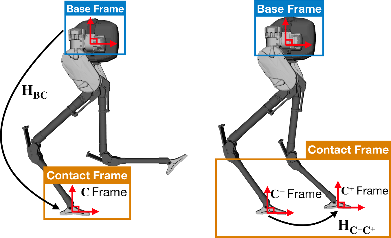
Figure 2: In this paper, we refer to two separate forward kinematics functions. The pose of the current contact frame relative to the base frame is denoted by H𝐦𝐢𝐬𝐬𝐢𝐧𝐠BCsubscriptHsubscript𝐦𝐢𝐬𝐬𝐢𝐧𝐠BC{}_{\text{}}\boldsymbol{\textbf{H}missing}_{\text{BC}}. When the robot has multiple points of contact with the environment, it is possible to transfer this contact from from one frame to another. This transfer of contact is captured by the homogeneous transform H𝐦𝐢𝐬𝐬𝐢𝐧𝐠C-C+subscriptHsubscript𝐦𝐢𝐬𝐬𝐢𝐧𝐠C-C+{}_{\text{}}\boldsymbol{\textbf{H}missing}_{\text{C\textsuperscript{-}C\textsuperscript{+}}}.

Let 𝜶N𝜶superscript𝑁\boldsymbol{\alpha}\in\mathbb{R}^{N} denote the vector of joint displacements for a general robot. Without loss of generality, we define a base frame on the robot, denoted B, that is assumed to be collocated with both the IMU and the camera frames. When the robot is in contact with the static environment, we can also define a contact frame, denoted C, on the robot at the point of contact. The homogeneous transformation between the base frame and the contact frame is defined by:

H𝐦𝐢𝐬𝐬𝐢𝐧𝐠BC(𝜶)[RBC(𝜶)pBCB(𝜶)01×31],subscriptHsubscript𝐦𝐢𝐬𝐬𝐢𝐧𝐠BC𝜶matrixsubscriptRBC𝜶subscriptsubscriptpBCB𝜶subscript0131{}_{\text{}}\boldsymbol{\textbf{H}missing}_{\text{BC}}(\boldsymbol{\alpha})\triangleq\begin{bmatrix}\textbf{R}_{\text{BC}}(\boldsymbol{\alpha})&{}_{\text{B}}\textbf{p}_{\text{BC}}(\boldsymbol{\alpha})\\ \textbf{0}_{1\times 3}&1\end{bmatrix}, (5)

where RBC(𝜶)subscriptRBC𝜶\textbf{R}_{\text{BC}}(\boldsymbol{\alpha}) and pBCB(𝜶)subscriptsubscriptpBCB𝜶{}_{\text{B}}\textbf{p}_{\text{BC}}(\boldsymbol{\alpha}) denote the relative orientation and position of the contact frame with respect to the base frame.

When there are two points in contact with the static environment, it is possible to “transfer” the contact frame from one point to the other (shown in Figure 2). Let CsuperscriptC\text{C}^{-} denote the old contact frame and C+superscriptC\text{C}^{+} denote the new contact frame. Then, the homogeneous transformation between the old frame and the new frame is defined by:

H𝐦𝐢𝐬𝐬𝐢𝐧𝐠C-C+(𝜶)[RC-C+(𝜶)pC-C+C-(𝜶)01×31],subscriptHsubscript𝐦𝐢𝐬𝐬𝐢𝐧𝐠C-C+𝜶matrixsubscriptRC-C+𝜶subscriptsubscriptpC-C+C-𝜶subscript0131{}_{\text{}}\boldsymbol{\textbf{H}missing}_{\text{C\textsuperscript{-}C\textsuperscript{+}}}(\boldsymbol{\alpha})\triangleq\begin{bmatrix}\textbf{R}_{\text{C\textsuperscript{-}C\textsuperscript{+}}}(\boldsymbol{\alpha})&{}_{\text{C\textsuperscript{-}}}\textbf{p}_{\text{C\textsuperscript{-}C\textsuperscript{+}}}(\boldsymbol{\alpha})\\ \textbf{0}_{1\times 3}&1\end{bmatrix}, (6)

where RC-C+(𝜶)subscriptRC-C+𝜶\textbf{R}_{\text{C\textsuperscript{-}C\textsuperscript{+}}}(\boldsymbol{\alpha}) and pC-C+C-(𝜶)subscriptsubscriptpC-C+C-𝜶{}_{\text{C\textsuperscript{-}}}\textbf{p}_{\text{C\textsuperscript{-}C\textsuperscript{+}}}(\boldsymbol{\alpha}) denote the relative orientation and position of the new contact frame with respect to the old contact frame.

IV-A Measurements

We assume the robot’s joints are equipped with a set of joint encoders that can measure the joint displacement. These encoder measurements, 𝜶~~𝜶\tilde{\boldsymbol{\alpha}}, are assumed to be corrupted with Gaussian white noise. This is an explicit measurement coming from physical sensors located on the robot.

𝜶~(t)=𝜶(t)+wα(t),wα(t)𝒩(0N×1,𝚺α(t))formulae-sequence~𝜶𝑡𝜶𝑡superscriptw𝛼𝑡similar-tosuperscriptw𝛼𝑡𝒩subscript0𝑁1superscript𝚺𝛼𝑡\tilde{\boldsymbol{\alpha}}(t)=\boldsymbol{\alpha}(t)+\textbf{w}^{\alpha}(t),\quad\textbf{w}^{\alpha}(t)\sim\mathcal{N}(\textbf{0}_{N\times 1},\boldsymbol{\Sigma}^{\alpha}(t))\\ (7)

The geometric (or manipulator) Jacobian, denoted J𝐦𝐢𝐬𝐬𝐢𝐧𝐠(𝜶)subscriptJsubscript𝐦𝐢𝐬𝐬𝐢𝐧𝐠𝜶{}_{\text{}}\boldsymbol{\textbf{J}missing}_{\text{}}(\boldsymbol{\alpha}), provides a method for computing the angular and linear velocity of an end-effector given the vector of joint velocities [19]. In a similar manner, we can use the Jacobian to map incremental angle displacements to changes in the end-effector pose. Let J𝐦𝐢𝐬𝐬𝐢𝐧𝐠BC(𝜶)subscriptJsubscript𝐦𝐢𝐬𝐬𝐢𝐧𝐠BC𝜶{}_{\text{}}\boldsymbol{\textbf{J}missing}_{\text{BC}}(\boldsymbol{\alpha}) denote the body manipulator Jacobian of the forward kinematics function (5). Then, the following relationship holds:

𝝃BCCδt=J𝐦𝐢𝐬𝐬𝐢𝐧𝐠BC(𝜶)δ𝜶subscriptsubscript𝝃BCC𝛿𝑡subscriptJsubscript𝐦𝐢𝐬𝐬𝐢𝐧𝐠BC𝜶𝛿𝜶{}_{\text{C}}\boldsymbol{\xi}_{\text{BC}}\,\delta t={}_{\text{}}\boldsymbol{\textbf{J}missing}_{\text{BC}}(\boldsymbol{\alpha})\,\delta\boldsymbol{\alpha} (8)

where δ𝜶𝛿𝜶\delta\boldsymbol{\alpha} and δt𝛿𝑡\delta t are incremental encoder and time quantities and 𝝃BCCsubscriptsubscript𝝃BCC{}_{\text{C}}\boldsymbol{\xi}_{\text{BC}} denotes the vector of angular and linear velocities of the contact frame due to δ𝜶𝛿𝜶\delta\boldsymbol{\alpha} (measured in the contact frame). We can use this relationship (8) to factor out the noise from the forward kinematics equations. Up to a first order approximation, (5) can be factored as:

H𝐦𝐢𝐬𝐬𝐢𝐧𝐠BC(𝜶(t))H𝐦𝐢𝐬𝐬𝐢𝐧𝐠BC(𝜶~(t))Exp(J𝐦𝐢𝐬𝐬𝐢𝐧𝐠BC(𝜶~(t))wα(t)).subscriptHsubscript𝐦𝐢𝐬𝐬𝐢𝐧𝐠BC𝜶𝑡subscriptHsubscript𝐦𝐢𝐬𝐬𝐢𝐧𝐠BC~𝜶𝑡ExpsubscriptJsubscript𝐦𝐢𝐬𝐬𝐢𝐧𝐠BC~𝜶𝑡superscriptw𝛼𝑡{}_{\text{}}\boldsymbol{\textbf{H}missing}_{\text{BC}}(\boldsymbol{\alpha}(t))\approx{}_{\text{}}\boldsymbol{\textbf{H}missing}_{\text{BC}}(\tilde{\boldsymbol{\alpha}}(t))\;\mathrm{Exp}\left(-{}_{\text{}}\boldsymbol{\textbf{J}missing}_{\text{BC}}(\tilde{\boldsymbol{\alpha}}(t))\textbf{w}^{\alpha}(t)\right).

(9)

A similar approximation can be found for (6), albeit with a different Jacobian.

H𝐦𝐢𝐬𝐬𝐢𝐧𝐠C-C+(𝜶(t))H𝐦𝐢𝐬𝐬𝐢𝐧𝐠C-C+(𝜶~(t))Exp(J𝐦𝐢𝐬𝐬𝐢𝐧𝐠C-C+(𝜶~(t))wα(t))subscriptHsubscript𝐦𝐢𝐬𝐬𝐢𝐧𝐠C-C+𝜶𝑡subscriptHsubscript𝐦𝐢𝐬𝐬𝐢𝐧𝐠C-C+~𝜶𝑡ExpsubscriptJsubscript𝐦𝐢𝐬𝐬𝐢𝐧𝐠C-C+~𝜶𝑡superscriptw𝛼𝑡{}_{\text{}}\boldsymbol{\textbf{H}missing}_{\text{C\textsuperscript{-}C\textsuperscript{+}}}(\boldsymbol{\alpha}(t))\approx{}_{\text{}}\boldsymbol{\textbf{H}missing}_{\text{C\textsuperscript{-}C\textsuperscript{+}}}(\tilde{\boldsymbol{\alpha}}(t))\;\mathrm{Exp}\left(-{}_{\text{}}\boldsymbol{\textbf{J}missing}_{\text{C\textsuperscript{-}C\textsuperscript{+}}}(\tilde{\boldsymbol{\alpha}}(t))\textbf{w}^{\alpha}(t)\right)

(10)
Remark 1.

In general, the manipulator Jacobian can be derived as spatial or body Jacobian [19], and based on this choice, the noise can appear on the left or right side of the rotation/rigid body transformation, respectively.

IV-B Forward Kinematic Factor

The goal of this section is to derive a general forward kinematic factor that can be used in the factor graph framework. This will be a unary factor that relates two poses through the forward kinematics equations while accounting for encoder noise. We derive it here for relating the base and contact frames.

The orientation and position of the contact frame with respect to the world frame are given by:

H𝐦𝐢𝐬𝐬𝐢𝐧𝐠WC(t)=H𝐦𝐢𝐬𝐬𝐢𝐧𝐠WB(t)H𝐦𝐢𝐬𝐬𝐢𝐧𝐠BC(𝜶(t)).subscriptHsubscript𝐦𝐢𝐬𝐬𝐢𝐧𝐠WC𝑡subscriptHsubscript𝐦𝐢𝐬𝐬𝐢𝐧𝐠WB𝑡subscriptHsubscript𝐦𝐢𝐬𝐬𝐢𝐧𝐠BC𝜶𝑡{}_{\text{}}\boldsymbol{\textbf{H}missing}_{\text{WC}}(t)={}_{\text{}}\boldsymbol{\textbf{H}missing}_{\text{WB}}(t)\;{}_{\text{}}\boldsymbol{\textbf{H}missing}_{\text{BC}}(\boldsymbol{\alpha}(t)). (11)

Substituting in the state variables at time tisubscript𝑡𝑖t_{i} (4), the forward kinematic equation (5) yields:

Ci=XiH𝐦𝐢𝐬𝐬𝐢𝐧𝐠BC(𝜶~iwiα).subscriptC𝑖subscriptX𝑖subscriptHsubscript𝐦𝐢𝐬𝐬𝐢𝐧𝐠BCsubscript~𝜶𝑖superscriptsubscriptw𝑖𝛼\textbf{C}_{i}=\textbf{X}_{i}\;{}_{\text{}}\boldsymbol{\textbf{H}missing}_{\text{BC}}(\tilde{\boldsymbol{\alpha}}_{i}-\textbf{w}_{i}^{\alpha}). (12)

We can now use the first order approximation (9) to factor out the encoder noise to give the following expression:

Ci=XiH𝐦𝐢𝐬𝐬𝐢𝐧𝐠BC(𝜶~i)Exp(J𝐦𝐢𝐬𝐬𝐢𝐧𝐠BC(𝜶~i)wiα).subscriptC𝑖subscriptX𝑖subscriptHsubscript𝐦𝐢𝐬𝐬𝐢𝐧𝐠BCsubscript~𝜶𝑖ExpsubscriptJsubscript𝐦𝐢𝐬𝐬𝐢𝐧𝐠BCsubscript~𝜶𝑖superscriptsubscriptw𝑖𝛼\textbf{C}_{i}=\textbf{X}_{i}\;{}_{\text{}}\boldsymbol{\textbf{H}missing}_{\text{BC}}(\tilde{\boldsymbol{\alpha}}_{i})\;\mathrm{Exp}\left(-{}_{\text{}}\boldsymbol{\textbf{J}missing}_{\text{BC}}(\tilde{\boldsymbol{\alpha}}_{i})\textbf{w}_{i}^{\alpha}\right). (13)

Defining the zero-mean white Gaussian forward kinematic noise term, δciJ𝐦𝐢𝐬𝐬𝐢𝐧𝐠BC(𝜶~i)wiα𝛿subscriptc𝑖subscriptJsubscript𝐦𝐢𝐬𝐬𝐢𝐧𝐠BCsubscript~𝜶𝑖superscriptsubscriptw𝑖𝛼\delta\textbf{c}_{i}\triangleq{}_{\text{}}\boldsymbol{\textbf{J}missing}_{\text{BC}}(\tilde{\boldsymbol{\alpha}}_{i})\textbf{w}_{i}^{\alpha}, allows us to write out the forward kinematic measurement model:

H𝐦𝐢𝐬𝐬𝐢𝐧𝐠BC(𝜶~i)=Xi1CiExp(δci),subscriptHsubscript𝐦𝐢𝐬𝐬𝐢𝐧𝐠BCsubscript~𝜶𝑖superscriptsubscriptX𝑖1subscriptC𝑖Exp𝛿subscriptc𝑖{}_{\text{}}\boldsymbol{\textbf{H}missing}_{\text{BC}}(\tilde{\boldsymbol{\alpha}}_{i})=\textbf{X}_{i}^{-1}\;\textbf{C}_{i}\;\mathrm{Exp}(\delta\textbf{c}_{i}), (14)

where the forward kinematic noise is characterized by δci𝒩(06×1,𝚺i)similar-to𝛿subscriptc𝑖𝒩subscript061subscript𝚺subscript𝑖\delta\textbf{c}_{i}\sim\mathcal{N}(\textbf{0}_{6\times 1},\boldsymbol{\Sigma}_{\mathcal{F}_{i}}). The residual error is defined in the tangent space and can be written as:

ri=Log(Ci1XiH𝐦𝐢𝐬𝐬𝐢𝐧𝐠BC(𝜶~i)).subscriptr𝑖LogsuperscriptsubscriptC𝑖1subscriptX𝑖subscriptHsubscript𝐦𝐢𝐬𝐬𝐢𝐧𝐠BCsubscript~𝜶𝑖\textbf{r}_{\mathcal{F}{i}}=\mathrm{Log}\left(\textbf{C}_{i}^{-1}\;\textbf{X}_{i}\;{}_{\text{}}\boldsymbol{\textbf{H}missing}_{\text{BC}}(\tilde{\boldsymbol{\alpha}}_{i})\right). (15)

The covariance is computed through the following linear transformation:

𝚺i=J𝐦𝐢𝐬𝐬𝐢𝐧𝐠BC(𝜶~i)𝚺iαJ𝐦𝐢𝐬𝐬𝐢𝐧𝐠BC𝖳(𝜶~i),subscript𝚺subscript𝑖subscriptJsubscript𝐦𝐢𝐬𝐬𝐢𝐧𝐠BCsubscript~𝜶𝑖superscriptsubscript𝚺𝑖𝛼subscriptJsuperscriptsubscript𝐦𝐢𝐬𝐬𝐢𝐧𝐠BC𝖳subscript~𝜶𝑖\boldsymbol{\Sigma}_{\mathcal{F}_{i}}={}_{\text{}}\boldsymbol{\textbf{J}missing}_{\text{BC}}(\tilde{\boldsymbol{\alpha}}_{i})\;\boldsymbol{\Sigma}_{i}^{\alpha}\;{}_{\text{}}\boldsymbol{\textbf{J}missing}_{\text{BC}}^{\mathsf{T}}(\tilde{\boldsymbol{\alpha}}_{i}), (16)

where J𝐦𝐢𝐬𝐬𝐢𝐧𝐠BC(𝜶~i)subscriptJsubscript𝐦𝐢𝐬𝐬𝐢𝐧𝐠BCsubscript~𝜶𝑖{}_{\text{}}\boldsymbol{\textbf{J}missing}_{\text{BC}}(\tilde{\boldsymbol{\alpha}}_{i}) is the body manipulator Jacobian evaluated at the current encoder measurements and 𝚺iαsuperscriptsubscript𝚺𝑖𝛼\boldsymbol{\Sigma}_{i}^{\alpha} denotes the encoder covariance matrix at time tisubscript𝑡𝑖t_{i}.

V Hybrid Contact Preintegration

A continuous hybrid dynamical system, \mathcal{H}, can be defined with a continuous dynamics function, f()𝑓f(\cdot), a discrete transition map, Δ()Δ\Delta(\cdot), and a switching surface, 𝒮𝒮\mathcal{S} [23]. Trajectories of the hybrid dynamical system evolve according to the continuous dynamics, until the switching surface it hit. At those moments, the state gets mapped through the discrete transition map, after which the trajectory continues according to the continuous dynamics again. The general form of this system can be expressed as follows:

:{x˙(t)=f(x,t)(x,t)𝒮x+=Δ(x)(x,t)𝒮.:cases˙𝑥𝑡formulae-sequenceabsent𝑓𝑥𝑡superscript𝑥superscript𝑡𝒮superscript𝑥formulae-sequenceabsentΔsuperscript𝑥superscript𝑥superscript𝑡𝒮otherwise\mathcal{H}:\begin{cases}\begin{aligned} \dot{x}(t)&=f(x,t)\qquad(x^{-},t^{-})\not\in\mathcal{S}\\ x^{+}&=\Delta(x^{-})\qquad(x^{-},t^{-})\in\mathcal{S}.\\ \end{aligned}\end{cases} (17)

As long as the number of contact points is greater than or equal to one, the switching contact frame dynamics can be modeled as a hybrid system:

:{H˙WC(t)=H𝐦𝐢𝐬𝐬𝐢𝐧𝐠WC(t)(𝝃WCC(t))t𝒮H𝐦𝐢𝐬𝐬𝐢𝐧𝐠WC+=H𝐦𝐢𝐬𝐬𝐢𝐧𝐠WC-H𝐦𝐢𝐬𝐬𝐢𝐧𝐠C-C+t𝒮,:casessubscript˙HWC𝑡absentsubscriptHsubscript𝐦𝐢𝐬𝐬𝐢𝐧𝐠WC𝑡superscriptsubscriptsubscript𝝃WCC𝑡missing-subexpressionsuperscript𝑡𝒮subscriptHsubscript𝐦𝐢𝐬𝐬𝐢𝐧𝐠WC+absentsubscriptHsubscript𝐦𝐢𝐬𝐬𝐢𝐧𝐠WC-subscriptHsubscript𝐦𝐢𝐬𝐬𝐢𝐧𝐠C-C+missing-subexpressionsuperscript𝑡𝒮otherwise\mathcal{H}:\begin{cases}\begin{aligned} \dot{\textbf{H}}_{\text{WC}}(t)&={}_{\text{}}\boldsymbol{\textbf{H}missing}_{\text{WC}}(t)\;\left({}_{\text{C}}\boldsymbol{\xi}_{\text{WC}}(t)\right)^{\wedge}\quad&&t^{-}\not\in\mathcal{S}\\ {}_{\text{}}\boldsymbol{\textbf{H}missing}_{\text{WC\textsuperscript{+}}}&={}_{\text{}}\boldsymbol{\textbf{H}missing}_{\text{WC\textsuperscript{-}}}\;{}_{\text{}}\boldsymbol{\textbf{H}missing}_{\text{C\textsuperscript{-}C\textsuperscript{+}}}\quad&&t^{-}\in\mathcal{S},\\ \end{aligned}\end{cases} (18)

where the switching surface, 𝒮𝒮\mathcal{S} is simply modeled as the set of all times where contact is switched from one frame to another. Since the sensor measurements are coming in at discrete time-steps, we perform Euler integration from time t𝑡t to t+Δt𝑡Δ𝑡t+\Delta t to discretize the continuous hybrid contact dynamics (18), forming the following discrete hybrid system:

:{H𝐦𝐢𝐬𝐬𝐢𝐧𝐠WC(t+Δt)=H𝐦𝐢𝐬𝐬𝐢𝐧𝐠WC(t)Exp(𝝃WCC(t)Δt)t𝒮H𝐦𝐢𝐬𝐬𝐢𝐧𝐠WC+=H𝐦𝐢𝐬𝐬𝐢𝐧𝐠WC-H𝐦𝐢𝐬𝐬𝐢𝐧𝐠C-C+t𝒮.:casessubscriptHsubscript𝐦𝐢𝐬𝐬𝐢𝐧𝐠WC𝑡Δ𝑡absentsubscriptHsubscript𝐦𝐢𝐬𝐬𝐢𝐧𝐠WC𝑡Expsubscriptsubscript𝝃WCC𝑡Δ𝑡missing-subexpressionsuperscript𝑡𝒮subscriptHsubscript𝐦𝐢𝐬𝐬𝐢𝐧𝐠WC+absentsubscriptHsubscript𝐦𝐢𝐬𝐬𝐢𝐧𝐠WC-subscriptHsubscript𝐦𝐢𝐬𝐬𝐢𝐧𝐠C-C+missing-subexpressionsuperscript𝑡𝒮otherwise\mathcal{H}:\begin{cases}\begin{aligned} {}_{\text{}}\boldsymbol{\textbf{H}missing}_{\text{WC}}(t+\Delta t)&={}_{\text{}}\boldsymbol{\textbf{H}missing}_{\text{WC}}(t)\;\mathrm{Exp}\left({}_{\text{C}}\boldsymbol{\xi}_{\text{WC}}(t)\Delta t\right)&&t^{-}\not\in\mathcal{S}\\ {}_{\text{}}\boldsymbol{\textbf{H}missing}_{\text{WC\textsuperscript{+}}}&={}_{\text{}}\boldsymbol{\textbf{H}missing}_{\text{WC\textsuperscript{-}}}\;{}_{\text{}}\boldsymbol{\textbf{H}missing}_{\text{C\textsuperscript{-}C\textsuperscript{+}}}&&t^{-}\in\mathcal{S}.\\ \end{aligned}\end{cases} (19)

Physically, the continuous dynamics function, f𝑓f, describes how a single contact frame moves over time while contact is maintained. When a new contact frame is detected, the new contact pose can be computed by applying the transition map, Δ()Δ\Delta(\cdot), which describes the homogeneous transformation between the old and new contact frames.

V-A Measurements

The angular and linear velocity of the contact point is an implicit measurement that is inferred through a binary contact sensor: specifically, when this sensor indicates contact, the pose of the contact frame is assumed to remain fixed with respect to the world frame, i.e. the measured velocities are zero. In order to accommodate potential contact slip, this measured twist is modeled to be corrupted with white Gaussian noise, namely

𝝃~WCC(t)=06×1=𝝃WCC(t)+wξ(t),wξ(t)𝒩(06×1,𝚺ξ(t)).formulae-sequencesubscriptsubscript~𝝃WCC𝑡subscript061subscriptsubscript𝝃WCC𝑡superscriptw𝜉𝑡similar-tosuperscriptw𝜉𝑡𝒩subscript061superscript𝚺𝜉𝑡{}_{\text{C}}\tilde{\boldsymbol{\xi}}_{\text{WC}}(t)=\textbf{0}_{6\times 1}={}_{\text{C}}\boldsymbol{\xi}_{\text{WC}}(t)+\textbf{w}^{\xi}(t),\hskip 5.69054pt\textbf{w}^{\xi}(t)\sim\mathcal{N}(\textbf{0}_{6\times 1},\boldsymbol{\Sigma}^{\xi}(t)).

Using the state variables (4), forward kinematics definition (6), encoder measurements (7), and contact measurements, the hybrid contact dynamics (19) can be written as:

:{Ck+1=CkExp(wkξdΔt)tk𝒮C+=CH𝐦𝐢𝐬𝐬𝐢𝐧𝐠C-C+(𝜶~kwkα)tk𝒮:casessubscriptC𝑘1absentsubscriptC𝑘Expsuperscriptsubscriptw𝑘𝜉𝑑Δ𝑡missing-subexpressionsuperscriptsubscript𝑡𝑘𝒮superscriptCabsentsuperscriptCsubscriptHsubscript𝐦𝐢𝐬𝐬𝐢𝐧𝐠C-C+subscript~𝜶𝑘superscriptsubscriptw𝑘𝛼missing-subexpressionsuperscriptsubscript𝑡𝑘𝒮otherwise\small\mathcal{H}:\begin{cases}\begin{aligned} \textbf{C}_{k+1}&=\textbf{C}_{k}\;\mathrm{Exp}\left(-\textbf{w}_{k}^{\xi d}\Delta t\right)\quad&&t_{k}^{-}\not\in\mathcal{S}\\ \textbf{C}^{+}&=\textbf{C}^{-}\;{}_{\text{}}\boldsymbol{\textbf{H}missing}_{\text{C\textsuperscript{-}C\textsuperscript{+}}}(\tilde{\boldsymbol{\alpha}}_{k}-\textbf{w}_{k}^{\alpha})\quad&&t_{k}^{-}\in\mathcal{S}\\ \end{aligned}\end{cases} (20)

where wkvdsuperscriptsubscriptw𝑘𝑣𝑑\textbf{w}_{k}^{vd}, the discrete time contact noise, is computed using the sample time, 𝐂𝐨𝐯[wξd(t)]=1Δt𝐂𝐨𝐯[wξ(t)]𝐂𝐨𝐯delimited-[]superscriptw𝜉𝑑𝑡1Δ𝑡𝐂𝐨𝐯delimited-[]superscriptw𝜉𝑡\small\mathbf{Cov}[\textbf{w}^{\xi d}(t)]=\dfrac{1}{\Delta t}\mathbf{Cov}[\textbf{w}^{\xi}(t)].

Remark 2.

H𝐦𝐢𝐬𝐬𝐢𝐧𝐠C-C+(𝜶k)subscriptHsubscript𝐦𝐢𝐬𝐬𝐢𝐧𝐠C-C+subscript𝜶𝑘{}_{\text{}}\boldsymbol{\textbf{H}missing}_{\text{C\textsuperscript{-}C\textsuperscript{+}}}(\boldsymbol{\alpha}_{k}) will depend on the specific contact frames, Csuperscript𝐶C^{-} and C+superscript𝐶C^{+}, at time tksubscript𝑡𝑘t_{k}. For example, the forward kinematics function to switch from left foot contact to a right foot contact will be different than the one used to switch from right foot to left foot.

V-B Preintegrating Contact Pose

The goal of this section is to formulate a general hybrid preintegrated contact factor which relates the contact pose at tisubscript𝑡𝑖t_{i} to the contact pose at tjsubscript𝑡𝑗t_{j}. The hybrid nature of this factor comes from the potential switching of contact that occurs naturally in legged locomotion. Following the work on IMU preintegration theory [24, 6], we preintegrate the high-frequency contact measurements to prevent unnecessary computation allowing efficient implementation of the factor.
Refer to caption
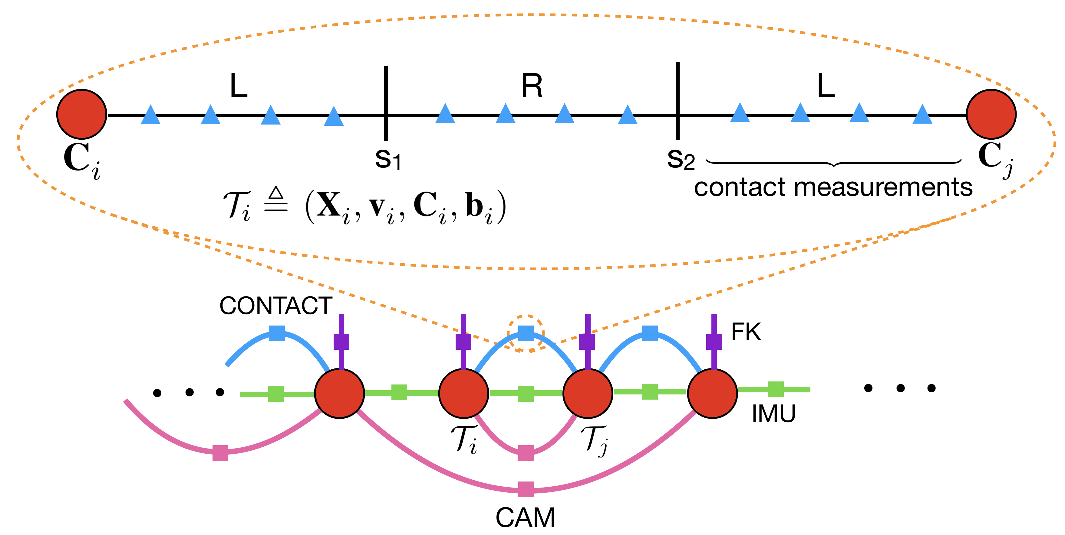
Figure 3: In the factor graph framework, the robot’s state along a discretized trajectory denoted by red circles. Each independent sensor measurement is a factor denoted by lines that constraints the state at separate time-steps. The proposed hybrid contact factor (shown on top) allows preintegration of high-frequency contact data through an arbitrary number of contact switches. In this example, there are two contact switches, where the robot moves from left-stance (L) to right-stance (R), then back to left stance.

Let 𝒮𝒮\mathcal{S} denote the sequence of all time indices associated with contact switches, so that each si𝒮subscript𝑠𝑖𝒮s_{i}\in\mathcal{S} represents a single time index where a contact switch occurs. To integrate the hybrid contact dynamics model (20) through these contact switches, we integrate the up to the next contact switch time tsisubscript𝑡subscript𝑠𝑖t_{s_{i}}, apply the transition map Δ()Δ\Delta(\cdot), and continue the integration. For the following derivations, a concrete example (depicted in Figure 3) is used to make the derivation easier to follow. We later extend the derivation to an arbitrary number of contact switches. For the example shown in Figure 3, there are two contact switches between times tisubscript𝑡𝑖t_{i} and tjsubscript𝑡𝑗t_{j}, i.e., |𝒮|=2𝒮2\lvert\mathcal{S}\rvert=2. Integrating the discrete hybrid contact model (20) from tisubscript𝑡𝑖t_{i} to tjsubscript𝑡𝑗t_{j} yields:

Cj=Ci(k=is11Exp(wkξdΔt))H𝐦𝐢𝐬𝐬𝐢𝐧𝐠C-C+(𝜶~s1ws1α)(k=s1s21Exp(wkξdΔt))H𝐦𝐢𝐬𝐬𝐢𝐧𝐠C-C+(𝜶~s2ws2α)(k=s2j1Exp(wkξdΔt)).subscriptC𝑗subscriptC𝑖superscriptsubscriptproduct𝑘𝑖subscript𝑠11Expsuperscriptsubscriptw𝑘𝜉𝑑Δ𝑡subscriptHsubscript𝐦𝐢𝐬𝐬𝐢𝐧𝐠C-C+subscript~𝜶subscript𝑠1superscriptsubscriptwsubscript𝑠1𝛼superscriptsubscriptproduct𝑘subscript𝑠1subscript𝑠21Expsuperscriptsubscriptw𝑘𝜉𝑑Δ𝑡subscriptHsubscript𝐦𝐢𝐬𝐬𝐢𝐧𝐠C-C+subscript~𝜶subscript𝑠2superscriptsubscriptwsubscript𝑠2𝛼superscriptsubscriptproduct𝑘subscript𝑠2𝑗1Expsuperscriptsubscriptw𝑘𝜉𝑑Δ𝑡\begin{split}&\textbf{C}_{j}=\textbf{C}_{i}\left(\prod_{k=i}^{s_{1}-1}\mathrm{Exp}(-\textbf{w}_{k}^{\xi d}\Delta t)\right){}_{\text{}}\boldsymbol{\textbf{H}missing}_{\text{C\textsuperscript{-}C\textsuperscript{+}}}(\tilde{\boldsymbol{\alpha}}_{s_{1}}-\textbf{w}_{s_{1}}^{\alpha})\\ &\left(\prod_{k=s_{1}}^{s_{2}-1}\mathrm{Exp}(-\textbf{w}_{k}^{\xi d}\Delta t)\right){}_{\text{}}\boldsymbol{\textbf{H}missing}_{\text{C\textsuperscript{-}C\textsuperscript{+}}}(\tilde{\boldsymbol{\alpha}}_{s_{2}}-\textbf{w}_{s_{2}}^{\alpha})\left(\prod_{k=s_{2}}^{j-1}\mathrm{Exp}(-\textbf{w}_{k}^{\xi d}\Delta t)\right).\\ \end{split}

All noise terms can be shifted to the right by using (10) to factor the noise from the forward kinematics term and the adjoint relation (2) to shift the measured kinematics to the left.

Cj=CiH𝐦𝐢𝐬𝐬𝐢𝐧𝐠C-C+(𝜶~s1)H𝐦𝐢𝐬𝐬𝐢𝐧𝐠C-C+(𝜶~s2)(k=is11Exp(AdH𝐦𝐢𝐬𝐬𝐢𝐧𝐠C-C+1(𝜶~s2)AdH𝐦𝐢𝐬𝐬𝐢𝐧𝐠C-C+1(𝜶~s1)wkξdΔt))Exp(AdH𝐦𝐢𝐬𝐬𝐢𝐧𝐠C-C+1(𝜶~s2)J𝐦𝐢𝐬𝐬𝐢𝐧𝐠C-C+(𝜶~s1)ws1α)(k=s1s21Exp(AdH𝐦𝐢𝐬𝐬𝐢𝐧𝐠C-C+1(𝜶~s2)wkξdΔt))Exp(J𝐦𝐢𝐬𝐬𝐢𝐧𝐠C-C+(𝜶~s2)ws2α)(k=s2j1Exp(wkξdΔt))subscriptC𝑗subscriptC𝑖subscriptHsubscript𝐦𝐢𝐬𝐬𝐢𝐧𝐠C-C+subscript~𝜶subscript𝑠1subscriptHsubscript𝐦𝐢𝐬𝐬𝐢𝐧𝐠C-C+subscript~𝜶subscript𝑠2superscriptsubscriptproduct𝑘𝑖subscript𝑠11ExpsubscriptAdsubscriptHsuperscriptsubscript𝐦𝐢𝐬𝐬𝐢𝐧𝐠C-C+1subscript~𝜶subscript𝑠2subscriptAdsubscriptHsuperscriptsubscript𝐦𝐢𝐬𝐬𝐢𝐧𝐠C-C+1subscript~𝜶subscript𝑠1superscriptsubscriptw𝑘𝜉𝑑Δ𝑡ExpsubscriptAdsubscriptHsuperscriptsubscript𝐦𝐢𝐬𝐬𝐢𝐧𝐠C-C+1subscript~𝜶subscript𝑠2subscriptJsubscript𝐦𝐢𝐬𝐬𝐢𝐧𝐠C-C+subscript~𝜶subscript𝑠1superscriptsubscriptwsubscript𝑠1𝛼superscriptsubscriptproduct𝑘subscript𝑠1subscript𝑠21ExpsubscriptAdsubscriptHsuperscriptsubscript𝐦𝐢𝐬𝐬𝐢𝐧𝐠C-C+1subscript~𝜶subscript𝑠2superscriptsubscriptw𝑘𝜉𝑑Δ𝑡ExpsubscriptJsubscript𝐦𝐢𝐬𝐬𝐢𝐧𝐠C-C+subscript~𝜶subscript𝑠2superscriptsubscriptwsubscript𝑠2𝛼superscriptsubscriptproduct𝑘subscript𝑠2𝑗1Expsuperscriptsubscriptw𝑘𝜉𝑑Δ𝑡\small\begin{split}&\textbf{C}_{j}=\textbf{C}_{i}\;{}_{\text{}}\boldsymbol{\textbf{H}missing}_{\text{C\textsuperscript{-}C\textsuperscript{+}}}(\tilde{\boldsymbol{\alpha}}_{s_{1}})\;{}_{\text{}}\boldsymbol{\textbf{H}missing}_{\text{C\textsuperscript{-}C\textsuperscript{+}}}(\tilde{\boldsymbol{\alpha}}_{s_{2}})\\ &\left(\prod_{k=i}^{s_{1}-1}\mathrm{Exp}(-\mathrm{Ad}_{{}_{\text{}}\boldsymbol{\textbf{H}missing}_{\text{C\textsuperscript{-}C\textsuperscript{+}}}^{-1}(\tilde{\boldsymbol{\alpha}}_{s_{2}})}\mathrm{Ad}_{{}_{\text{}}\boldsymbol{\textbf{H}missing}_{\text{C\textsuperscript{-}C\textsuperscript{+}}}^{-1}(\tilde{\boldsymbol{\alpha}}_{s_{1}})}\textbf{w}_{k}^{\xi d}\Delta t)\right)\\ &\mathrm{Exp}(-\mathrm{Ad}_{{}_{\text{}}\boldsymbol{\textbf{H}missing}_{\text{C\textsuperscript{-}C\textsuperscript{+}}}^{-1}(\tilde{\boldsymbol{\alpha}}_{s_{2}})}{}_{\text{}}\boldsymbol{\textbf{J}missing}_{\text{C\textsuperscript{-}C\textsuperscript{+}}}(\tilde{\boldsymbol{\alpha}}_{s_{1}})\textbf{w}_{s_{1}}^{\alpha})\\ &\left(\prod_{k=s_{1}}^{s_{2}-1}\mathrm{Exp}(-\mathrm{Ad}_{{}_{\text{}}\boldsymbol{\textbf{H}missing}_{\text{C\textsuperscript{-}C\textsuperscript{+}}}^{-1}(\tilde{\boldsymbol{\alpha}}_{s_{2}})}\textbf{w}_{k}^{\xi d}\Delta t)\right)\\ &\mathrm{Exp}(-{}_{\text{}}\boldsymbol{\textbf{J}missing}_{\text{C\textsuperscript{-}C\textsuperscript{+}}}(\tilde{\boldsymbol{\alpha}}_{s_{2}})\textbf{w}_{s_{2}}^{\alpha})\left(\prod_{k=s_{2}}^{j-1}\mathrm{Exp}(-\textbf{w}_{k}^{\xi d}\Delta t)\right)\\ \end{split} (21)

After multiplying both sides by Ci1superscriptsubscriptC𝑖1\textbf{C}_{i}^{-1}, we arrive at a relative pose expression that is independent of states 𝒯isubscript𝒯𝑖\mathcal{T}_{i} and 𝒯jsubscript𝒯𝑗\mathcal{T}_{j}.

ΔCijCi1Cj=ΔC~ijExp(δcij)ΔsubscriptC𝑖𝑗superscriptsubscriptC𝑖1subscriptC𝑗Δsubscript~C𝑖𝑗Exp𝛿subscriptc𝑖𝑗\Delta\textbf{C}_{ij}\triangleq\textbf{C}_{i}^{-1}\textbf{C}_{j}=\Delta\tilde{\textbf{C}}_{ij}\mathrm{Exp}(-\delta\textbf{c}_{ij})\\ (22)

where ΔC~ijn=1|𝒮|H𝐦𝐢𝐬𝐬𝐢𝐧𝐠C-C+(𝜶~sn)Δsubscript~C𝑖𝑗superscriptsubscriptproduct𝑛1𝒮subscriptHsubscript𝐦𝐢𝐬𝐬𝐢𝐧𝐠C-C+subscript~𝜶subscript𝑠𝑛\Delta\tilde{\textbf{C}}_{ij}\triangleq\prod_{n=1}^{|\mathcal{S}|}{}_{\text{}}\boldsymbol{\textbf{H}missing}_{\text{C\textsuperscript{-}C\textsuperscript{+}}}(\tilde{\boldsymbol{\alpha}}_{s_{n}}) represents the hybrid preintegrated contact measurement, and Exp(δcij)Exp𝛿subscriptc𝑖𝑗\mathrm{Exp}(-\delta\textbf{c}_{ij}) groups all of the noise terms together. This noise term is a product of multiple small rigid body transformations. Therefore, it can be approximated as a summation in the tangent space through iterative use of the Baker-Campbell-Hausdorff (BCH) formula [20] (while keeping only the first order terms).

δcijk=is11AdH𝐦𝐢𝐬𝐬𝐢𝐧𝐠C-C+1(𝜶~s2)AdH𝐦𝐢𝐬𝐬𝐢𝐧𝐠C-C+1(𝜶~s1)wkξdΔt+AdH𝐦𝐢𝐬𝐬𝐢𝐧𝐠C-C+1(𝜶~s2)J𝐦𝐢𝐬𝐬𝐢𝐧𝐠C-C+(𝜶~s1)ws1α+k=s1s21AdH𝐦𝐢𝐬𝐬𝐢𝐧𝐠C-C+1(𝜶~s2)wkξdΔt+J𝐦𝐢𝐬𝐬𝐢𝐧𝐠C-C+(𝜶~s2)ws2α+k=s2j1wkξdΔt𝛿subscriptc𝑖𝑗superscriptsubscript𝑘𝑖subscript𝑠11subscriptAdsubscriptHsuperscriptsubscript𝐦𝐢𝐬𝐬𝐢𝐧𝐠C-C+1subscript~𝜶subscript𝑠2subscriptAdsubscriptHsuperscriptsubscript𝐦𝐢𝐬𝐬𝐢𝐧𝐠C-C+1subscript~𝜶subscript𝑠1superscriptsubscriptw𝑘𝜉𝑑Δ𝑡subscriptAdsubscriptHsuperscriptsubscript𝐦𝐢𝐬𝐬𝐢𝐧𝐠C-C+1subscript~𝜶subscript𝑠2subscriptJsubscript𝐦𝐢𝐬𝐬𝐢𝐧𝐠C-C+subscript~𝜶subscript𝑠1superscriptsubscriptwsubscript𝑠1𝛼superscriptsubscript𝑘subscript𝑠1subscript𝑠21subscriptAdsubscriptHsuperscriptsubscript𝐦𝐢𝐬𝐬𝐢𝐧𝐠C-C+1subscript~𝜶subscript𝑠2superscriptsubscriptw𝑘𝜉𝑑Δ𝑡subscriptJsubscript𝐦𝐢𝐬𝐬𝐢𝐧𝐠C-C+subscript~𝜶subscript𝑠2superscriptsubscriptwsubscript𝑠2𝛼superscriptsubscript𝑘subscript𝑠2𝑗1superscriptsubscriptw𝑘𝜉𝑑Δ𝑡\begin{split}\small\delta&\textbf{c}_{ij}\approx\sum_{k=i}^{s_{1}-1}\mathrm{Ad}_{{}_{\text{}}\boldsymbol{\textbf{H}missing}_{\text{C\textsuperscript{-}C\textsuperscript{+}}}^{-1}(\tilde{\boldsymbol{\alpha}}_{s_{2}})}\mathrm{Ad}_{{}_{\text{}}\boldsymbol{\textbf{H}missing}_{\text{C\textsuperscript{-}C\textsuperscript{+}}}^{-1}(\tilde{\boldsymbol{\alpha}}_{s_{1}})}\textbf{w}_{k}^{\xi d}\Delta t\\ &+\mathrm{Ad}_{{}_{\text{}}\boldsymbol{\textbf{H}missing}_{\text{C\textsuperscript{-}C\textsuperscript{+}}}^{-1}(\tilde{\boldsymbol{\alpha}}_{s_{2}})}{}_{\text{}}\boldsymbol{\textbf{J}missing}_{\text{C\textsuperscript{-}C\textsuperscript{+}}}(\tilde{\boldsymbol{\alpha}}_{s_{1}})\textbf{w}_{s_{1}}^{\alpha}+\sum_{k=s_{1}}^{s_{2}-1}\mathrm{Ad}_{{}_{\text{}}\boldsymbol{\textbf{H}missing}_{\text{C\textsuperscript{-}C\textsuperscript{+}}}^{-1}(\tilde{\boldsymbol{\alpha}}_{s_{2}})}\textbf{w}_{k}^{\xi d}\Delta t\\ &+{}_{\text{}}\boldsymbol{\textbf{J}missing}_{\text{C\textsuperscript{-}C\textsuperscript{+}}}(\tilde{\boldsymbol{\alpha}}_{s_{2}})\textbf{w}_{s_{2}}^{\alpha}+\sum_{k=s_{2}}^{j-1}\textbf{w}_{k}^{\xi d}\Delta t\end{split}

The hybrid preintegrated contact noise, δcij𝛿subscriptc𝑖𝑗\delta\textbf{c}_{ij}, is a summation of zero-mean Gaussian terms, and is therefore also zero-mean and Gaussian. It is possible to generalize this noise expression to an arbitrary number of contact switches, however, it becomes much simpler to do so when looking at the iterative propagation form in the following section.

V-C Iterative Propagation

It is possible to write both the preintegrated contact measurements, ΔC~ijΔsubscript~C𝑖𝑗\Delta\tilde{\textbf{C}}_{ij}, and the preintegrated contact noise, δcij𝛿subscriptc𝑖𝑗\delta\textbf{c}_{ij}, in iterative update forms. This allows the terms to be updated as contact and encoder measurements are coming in. In addition, this form simplifies the expressions and allows for the covariance to be conveniently computed. The following proposition generalizes the hybrid preintegrated contact pose and noise iterative propagation to an arbitrary number of contact switches. The proof is given in the supplementary material.

Proposition 1 (Iterative Propagation of Hybrid Contact Process [25]).

Between any two time-steps tisubscripttit_{i} and tjsubscripttjt_{j} such that j>i𝑗𝑖j>i, starting with ΔC~ii=I4Δsubscript~CiisubscriptI4\Delta\tilde{\textbf{C}}_{ii}=\textbf{I}_{4} and δcii=03×1𝛿subscriptciisubscript031\delta\textbf{c}_{ii}=\textbf{0}_{3\times 1}, the hybrid preintegrated contact measurement, ΔC~ijΔsubscript~Cij\Delta\tilde{\textbf{C}}_{ij}, and noise, δcij𝛿subscriptcij\delta\textbf{c}_{ij}, for an arbitrary number of contact switches can be computed iteratively using the following hybrid systems:

~:{ΔC~ik+1=ΔC~iktk𝒮ΔC~ik+=ΔC~ikH𝐦𝐢𝐬𝐬𝐢𝐧𝐠C-C+(𝜶~k)tk𝒮:~casesΔsubscript~C𝑖𝑘1absentΔsubscript~C𝑖𝑘missing-subexpressionsuperscriptsubscript𝑡𝑘𝒮Δsuperscriptsubscript~C𝑖𝑘absentΔsuperscriptsubscript~C𝑖𝑘subscriptHsubscript𝐦𝐢𝐬𝐬𝐢𝐧𝐠C-C+subscript~𝜶𝑘missing-subexpressionsuperscriptsubscript𝑡𝑘𝒮otherwise\small\tilde{\mathcal{H}}:\begin{cases}\begin{aligned} \Delta\tilde{\textbf{C}}_{ik+1}&=\Delta\tilde{\textbf{C}}_{ik}\quad&&t_{k}^{-}\not\in\mathcal{S}\\ \Delta\tilde{\textbf{C}}_{ik}^{+}&=\Delta\tilde{\textbf{C}}_{ik}^{-}\;{}_{\text{}}\boldsymbol{\textbf{H}missing}_{\text{C\textsuperscript{-}C\textsuperscript{+}}}(\tilde{\boldsymbol{\alpha}}_{k})\quad&&t_{k}^{-}\in\mathcal{S}\\ \end{aligned}\end{cases} (23)
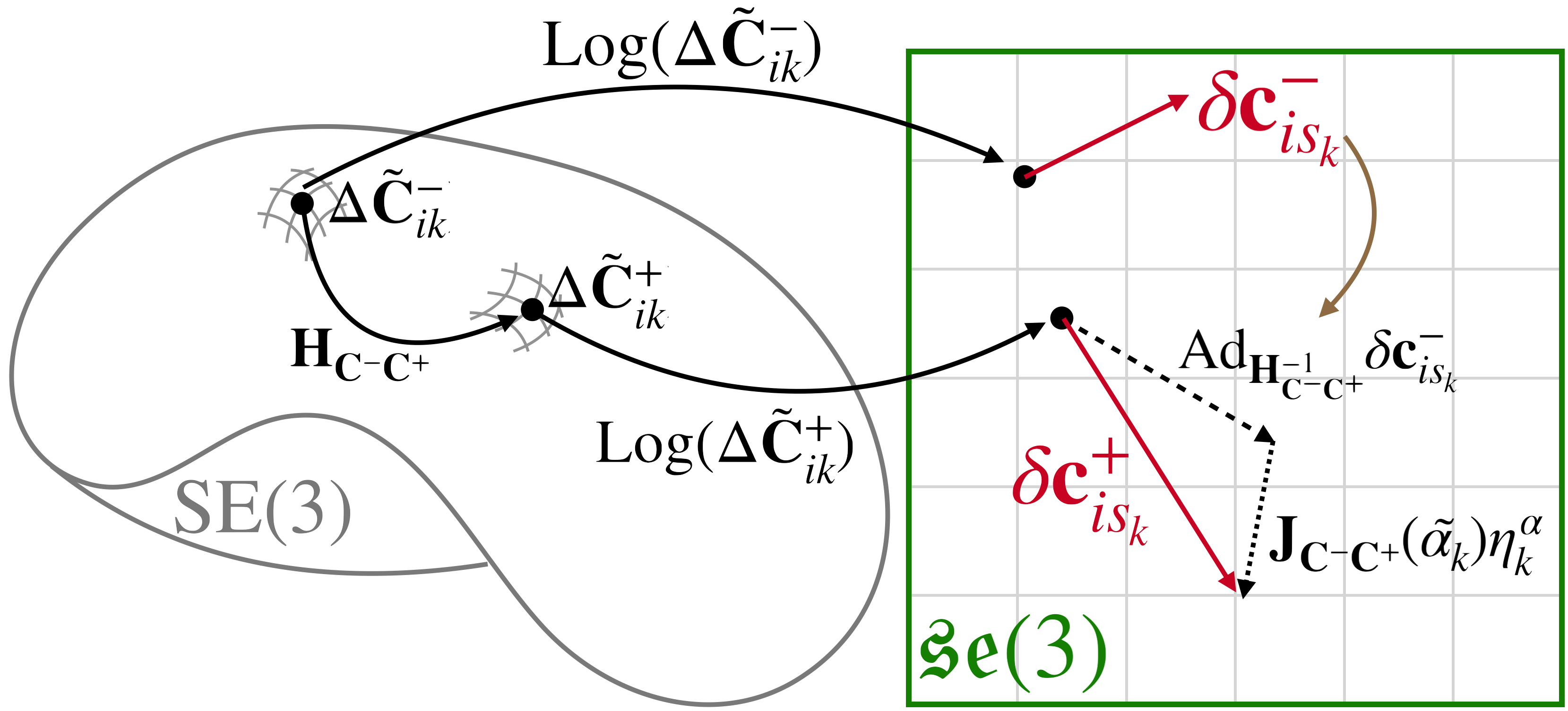
δ:{δcik+1=δcik+wkξdΔttk𝒮δcik+=AdH𝐦𝐢𝐬𝐬𝐢𝐧𝐠C-C+1(𝜶~k)δcik+J𝐦𝐢𝐬𝐬𝐢𝐧𝐠C-C+(𝜶~k)wkαtk𝒮:𝛿cases𝛿subscriptc𝑖𝑘1absent𝛿subscriptc𝑖𝑘superscriptsubscriptw𝑘𝜉𝑑Δ𝑡missing-subexpressionsuperscriptsubscript𝑡𝑘𝒮𝛿superscriptsubscriptc𝑖𝑘absentsubscriptAdsubscriptHsuperscriptsubscript𝐦𝐢𝐬𝐬𝐢𝐧𝐠C-C+1subscript~𝜶𝑘𝛿superscriptsubscriptc𝑖𝑘subscriptJsubscript𝐦𝐢𝐬𝐬𝐢𝐧𝐠C-C+subscript~𝜶𝑘superscriptsubscriptw𝑘𝛼missing-subexpressionsuperscriptsubscript𝑡𝑘𝒮otherwise\small\delta\mathcal{H}:\begin{cases}\begin{aligned} \delta\textbf{c}_{ik+1}&=\delta\textbf{c}_{ik}+\textbf{w}_{k}^{\xi d}\Delta t\quad&&t_{k}^{-}\not\in\mathcal{S}\\ \delta\textbf{c}_{ik}^{+}&=\mathrm{Ad}_{{}_{\text{}}\boldsymbol{\textbf{H}missing}_{\text{C\textsuperscript{-}C\textsuperscript{+}}}^{-1}(\tilde{\boldsymbol{\alpha}}_{k})}\delta\textbf{c}_{ik}^{-}+{}_{\text{}}\boldsymbol{\textbf{J}missing}_{\text{C\textsuperscript{-}C\textsuperscript{+}}}(\tilde{\boldsymbol{\alpha}}_{k})\textbf{w}_{k}^{\alpha}\quad&&t_{k}^{-}\in\mathcal{S}\end{aligned}\end{cases} (24)

An abstract representation of these hybrid systems is shown in Figure 4.
Refer to caption
Figure 4: When a contact switch occurs, the relative contact pose, ΔC~ikΔsuperscriptsubscript~C𝑖𝑘\scriptsize\Delta\tilde{\textbf{C}}_{ik}^{-}, gets mapped from one point in SE(3)SE3\mathrm{SE}(3) to another point, ΔC~ik+Δsuperscriptsubscript~C𝑖𝑘\scriptsize\Delta\tilde{\textbf{C}}_{ik}^{+}, on the manifold. The contact noise, δcik𝛿superscriptsubscriptc𝑖𝑘\scriptsize\delta\textbf{c}_{ik}^{-}, is represented in the tangent space, 𝔰𝔢(3)𝔰𝔢3\mathfrak{se}(3), and is mapped from the tangent space of ΔC~ikΔsuperscriptsubscript~C𝑖𝑘\scriptsize\Delta\tilde{\textbf{C}}_{ik}^{-} to the tangent space of ΔC~ik+Δsuperscriptsubscript~C𝑖𝑘\scriptsize\Delta\tilde{\textbf{C}}_{ik}^{+} through the use of the adjoint map of the forward kinematics transformation, H𝐦𝐢𝐬𝐬𝐢𝐧𝐠C-C+subscriptHsubscript𝐦𝐢𝐬𝐬𝐢𝐧𝐠C-C+\scriptsize{}_{\text{}}\boldsymbol{\textbf{H}missing}_{\text{C\textsuperscript{-}C\textsuperscript{+}}}. However, due to noisy encoders, an addition noise term (computed using the manipulator Jacobian) has to be added to compute δcik+𝛿superscriptsubscriptc𝑖𝑘\scriptsize\delta\textbf{c}_{ik}^{+}.

V-D Rigid Contact Factor

The relative contact pose expression (22) can be used to define the hybrid preintegrated contact measurement model:

ΔC~ij=Ci1CjExp(δcij),Δsubscript~C𝑖𝑗superscriptsubscriptC𝑖1subscriptC𝑗Exp𝛿subscriptc𝑖𝑗\Delta\tilde{\textbf{C}}_{ij}=\textbf{C}_{i}^{-1}\textbf{C}_{j}\mathrm{Exp}(\delta\textbf{c}_{ij}), (25)

where the preintegrated contact noise is characterized by δcij𝒩(06×1,𝚺𝒞ij)similar-to𝛿subscriptc𝑖𝑗𝒩subscript061subscript𝚺subscript𝒞𝑖𝑗\delta\textbf{c}_{ij}\sim\mathcal{N}(\textbf{0}_{6\times 1},\boldsymbol{\Sigma}_{\mathcal{C}_{ij}}). In the factor graph framework, this hybrid preintegrated contact model represents a binary factor that relates the contact frame pose over consecutive time steps. The residual error is defined in the tangent space, and can be written as:

r𝒞ij=Log(Cj1CiΔC~ij(𝜶~i)).subscriptrsubscript𝒞𝑖𝑗LogsuperscriptsubscriptC𝑗1subscriptC𝑖Δsubscript~C𝑖𝑗subscript~𝜶𝑖\textbf{r}_{\mathcal{C}_{ij}}=\mathrm{Log}\left(\textbf{C}_{j}^{-1}\textbf{C}_{i}\Delta\tilde{\textbf{C}}_{ij}(\tilde{\boldsymbol{\alpha}}_{i})\right). (26)

The covariance is computed using the hybrid contact noise model (24), starting with 𝚺𝒞ii=06×6subscript𝚺subscript𝒞𝑖𝑖subscript066\boldsymbol{\Sigma}_{\mathcal{C}_{ii}}=\textbf{0}_{6\times 6}:

{𝚺𝒞ik+1=𝚺𝒞ik+𝚺kξΔttk𝒮𝚺𝒞ik+=AdH𝐦𝐢𝐬𝐬𝐢𝐧𝐠C-C+1(𝜶~k)𝚺𝒞ikAdH𝐦𝐢𝐬𝐬𝐢𝐧𝐠C-C+1(𝜶~k)𝖳tk𝒮+J𝐦𝐢𝐬𝐬𝐢𝐧𝐠C-C+(𝜶~k)𝚺kαJ𝐦𝐢𝐬𝐬𝐢𝐧𝐠C-C+𝖳(𝜶~k).casessubscript𝚺subscript𝒞𝑖𝑘1absentsubscript𝚺subscript𝒞𝑖𝑘superscriptsubscript𝚺𝑘𝜉Δ𝑡missing-subexpressionsuperscriptsubscript𝑡𝑘𝒮superscriptsubscript𝚺subscript𝒞𝑖𝑘absentsubscriptAdsubscriptHsuperscriptsubscript𝐦𝐢𝐬𝐬𝐢𝐧𝐠C-C+1subscript~𝜶𝑘superscriptsubscript𝚺subscript𝒞𝑖𝑘superscriptsubscriptAdsubscriptHsuperscriptsubscript𝐦𝐢𝐬𝐬𝐢𝐧𝐠C-C+1subscript~𝜶𝑘𝖳missing-subexpressionsuperscriptsubscript𝑡𝑘𝒮missing-subexpressionsubscriptJsubscript𝐦𝐢𝐬𝐬𝐢𝐧𝐠C-C+subscript~𝜶𝑘superscriptsubscript𝚺𝑘𝛼subscriptJsuperscriptsubscript𝐦𝐢𝐬𝐬𝐢𝐧𝐠C-C+𝖳subscript~𝜶𝑘otherwise\small\begin{cases}\begin{aligned} \boldsymbol{\Sigma}_{\mathcal{C}_{ik+1}}&=\boldsymbol{\Sigma}_{\mathcal{C}_{ik}}+\boldsymbol{\Sigma}_{k}^{\xi}\;\Delta t\quad&&t_{k}^{-}\not\in\mathcal{S}\\ \boldsymbol{\Sigma}_{\mathcal{C}_{ik}}^{+}&=\mathrm{Ad}_{{}_{\text{}}\boldsymbol{\textbf{H}missing}_{\text{C\textsuperscript{-}C\textsuperscript{+}}}^{-1}\;(\tilde{\boldsymbol{\alpha}}_{k})}\boldsymbol{\Sigma}_{\mathcal{C}_{ik}}^{-}\;\mathrm{Ad}_{{}_{\text{}}\boldsymbol{\textbf{H}missing}_{\text{C\textsuperscript{-}C\textsuperscript{+}}}^{-1}(\tilde{\boldsymbol{\alpha}}_{k})}^{\mathsf{T}}\quad&&t_{k}^{-}\in\mathcal{S}\\ &\qquad\quad+{}_{\text{}}\boldsymbol{\textbf{J}missing}_{\text{C\textsuperscript{-}C\textsuperscript{+}}}(\tilde{\boldsymbol{\alpha}}_{k})\;\boldsymbol{\Sigma}_{k}^{\alpha}\;{}_{\text{}}\boldsymbol{\textbf{J}missing}_{\text{C\textsuperscript{-}C\textsuperscript{+}}}^{\mathsf{T}}(\tilde{\boldsymbol{\alpha}}_{k}).\end{aligned}\end{cases} (27)

VI Experimental Results

Refer to caption
(a)
Refer to caption
(b)
Refer to caption
(c)
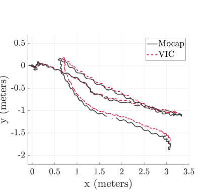
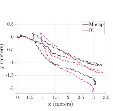
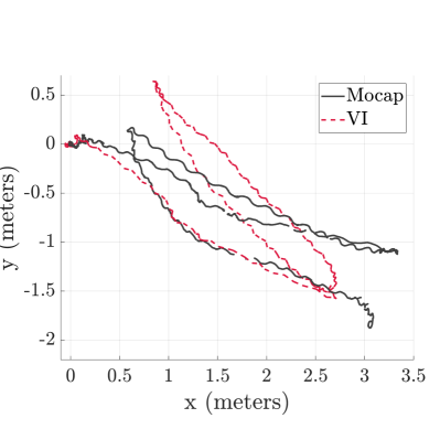
Figure 5: The odometry results from a 60 second walking experiment using a Cassie-series robot. The Visual-Inertial-Contact (VIC) odometry outperformed both the Inertial-Contact (IC), and the Visual-Inertial (VI) odometry. “Ground-truth” data was collected from a Vicon motion capture system. It is important to note that no loop-closures are being performed, which helps to explain the relatively poor odometry from VI. The video of this experiment is provided at https://youtu.be/WDPhdl5g2MQ.

We now present experimental evaluations of the proposed factors. In the first experiment, we compare three odometry systems composed by Visual-Inertial-Contact (VIC), Inertial-Contact (IC), and Visual-Inertial (VI) factors. Whenever the contact factor is used, it is assumed that forward kinematic factor is also available; therefore, it is not explicitly mentioned for brevity. In the second experiment, we study the effect of losing visual data for a period of time to see how the contact factor can constrain the graph in the absence of a reliable vision system. In the third experiment, we will evaluate the use of terrain factors, where loop-closures can be added to the graph through contact frame poses.

VI-A Experimental Setup

All experiments are done on a Cassie-series robot designed by Agility Robotics, which has 20 degrees of freedom, 10 actuators, joint encoders, and a VN-100 IMU. A Multisense S7 stereo camera, which contains a separate IMU, is mounted on the top of the Cassie robot as shown in Fig. 1. The robot also has four springs (two on each leg) that can be used as binary contact sensors by thresholding the spring deflection measurements. The Cassie robot has two computers which run MATLAB Simulink Real-Time (for the controller) and Ubuntu (for the estimator) respectively. We use the Robot Operating System (ROS) [26] with the User Datagram Protocol (UDP) to communicate sensor data between the two computers. We also integrate the time synchronization algorithm in [27] into our system to ensure all sensory data is synchronized.

The motion capture system developed by Vicon is used as a proxy for ground truth trajectories. The setup consists of 17 motion capture cameras with four markers attached to the robot to track the IMU pose. The dataset contains the stereo images (20Hz20Hz20\mathop{\mathrm{Hz}}) and IMU data (750Hz750Hz750\mathop{\mathrm{Hz}}) from the Multisense S7 camera as well as the joint encoders and IMU data from the Cassie robot (at 400Hz400Hz400\mathop{\mathrm{Hz}} each).

The proposed kinematic and contact factors were implemented using the GTSAM 4.0 library [4]. We utilized the built-in preintegrated IMU factor [6] with the iSAM2 [3] incremental solver. For visual odometry, we used the semi-direct visual odometry library (SVO 2.0 [28]). The Multisense camera recorded synchronized stereo images at 20Hz20Hz20\mathop{\mathrm{Hz}} and IMU measurements in about 750Hz750Hz750\mathop{\mathrm{Hz}}. SVO processes those measurements in real-time and outputs the pose of the left camera in a fixed world frame, XisubscriptX𝑖\textbf{X}_{i}, for the current time-step i𝑖i. The relative transformation of the camera from time-step i𝑖i to j𝑗j can be obtained using ΔXij=Xi1XjΔsubscriptX𝑖𝑗superscriptsubscriptX𝑖1subscriptX𝑗\Delta\textbf{X}_{ij}=\textbf{X}_{i}^{-1}\textbf{X}_{j}. We selected keyframes approximately every 0.250.250.25 seconds.

Refer to caption
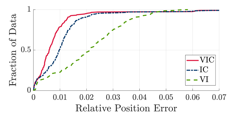
Figure 6: The Cumulative Distribution Function (CDF) of the relative position error provides a way to analyze the drift in the odometry estimates from various combinations of factors. The fraction of data corresponding to small relative position errors (low-drift odometry) is the larger for Visual-Inertial-Contact (VIC) odometry than for Inertial-Contact (IC) or Visual-Inertial (VI) odometry.
Refer to caption
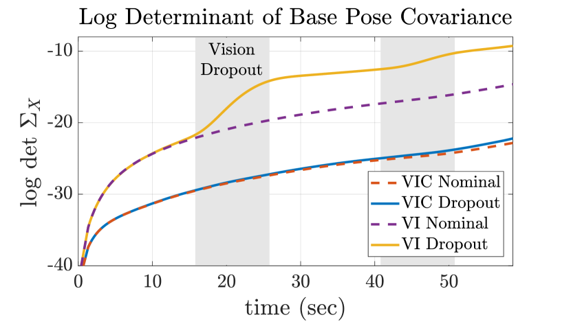
Figure 7: When vision data is lost, the covariance of the robot’s base pose sharply grows for VI odometry due to the lack of additional measurements to constrain the graph. In contrast, during “vision dropout” periods, the additional contact factors allows the covariance estimate from VIC to remains close to the nominal case.

VI-B First Experiment: Odometry Comparison

In this experiment, we had Cassie stand in place for about 15 seconds, then slowly walk forwards and backwards along the length of the lab for approximately 45 seconds. The resulting data was used to compare the odometry performance (processed off-line) of different combinations of factors. The results are shown in Figure 5. The odometry estimate from VIC, as expected, outperforms all other combinations of factors. The Cumulative Distribution Function (CDF) of the relative position error is shown in Figure 6. The relative position CDF provides a method for analyzing the drift of an odometry estimate.

From Figure 6, it can be seen that VIC has the highest fraction of data corresponding to smaller relative position errors. This means VIC has lowest drift among all odometry systems. When the robot is walking, the hard impacts cause significant camera shake which leads to motion blur in the images. In addition, the lab environment seemingly lacked numerous quality features. These effects help to explain the relatively poor VI odometry performance.

VI-C Second Experiment: Vision Dropout

One of the main benefits from including the forward kinematic and contact factors is that the state estimator can be more robust to failure of the vision system. In this experiment, we simulate the effects of “vision dropout” by simply ignoring SVO visual odometry data for two 10-second periods of the experimental data described in the previous section. In other words, during a “vision dropout” period, VIC odometry reduces to IC odometry, and VI odometry reduces down to inertial (I) odometry. Figure 7 shows the log determinant of the base pose covariance for VIC and VI for these “vision dropout” experiments. The larger the log determinant, the more uncertain the estimator is about the robot’s base pose. During the “vision dropout” periods, uncertainty grows for VI odometry. This sharp covariance growth is due to the lack of additional sensor measurements to add into the factor graph. In contrast, the covariance growth for VIC is hardly affected over the same dropout periods.

VI-D Third Experiment: Terrain Factors for Loop-Closure

Another benefit of adding the proposed contact factors comes from the addition of the contact frame poses into the robot’s state. With these new state variables, it becomes simple to place additional constraints that relate the contact pose to a prior map. We test this idea on the collected experiment data by recognizing that the ground was relatively flat in the laboratory. This “zero-height” elevation data serves as our prior map. Figure 8 shows how adding this trivial constraint can reduce position drift in the z-direction. This experiment simply serves to illustrate the potential for “terrain factors”, as the state estimate could be further improved if the robot was actually mapping out the terrain; there was actually a slight slope in the lab (as shown in the motion capture data).

Refer to caption
Figure 8: Since the contact pose is now part of the estimated state, it is possible to add “terrain factors” that relate this contact pose to a prior map. Adding the simple constraint that the contact frame z-translation is zero (VIC-T) improves the drift in the z-direction when compared to the nominal Visual-Inertial-Contact (VIC) case.

VII Conclusion

We developed a novel method for preintegrating contact information through an arbitrary number of contact switches using a hybrid preintegrated contact factor. The proposed approach was verified through experimental evaluations using a Cassie-series robot where a motion capture system is used as a proxy for ground truth data. Our results indicate that the fusion of contact information with IMU and vision data provide a reliable odometry system for legged robot. Furthermore, we showed that the developed visual-inertial-contact odometry system is robust to occasional vision system failures.

In the future, we plan to incorporate loop closure constraints into our factor graph framework to further improve state estimation, paving the way for long-term mapping on legged robots. We also plan to further investigate the potential utility of “terrain factors” to allow the robot’s state to be corrected though detected contact on an estimated map.

ACKNOWLEDGMENT

The authors thank Agility Robotics for designing the robot, and Yukai Gong for developing the feedback controller. We also thank Dr. Elliott Rouse and Catherine Kinnaird for providing us with the lab space and equipment necessary to collect and analyze the motion capture data. Funding for R. Hartley, M. Ghaffari Jadidi, L. Gan, and J. Huang is given by the Toyota Research Institute (TRI), partly under award number N021515, however this article solely reflects the opinions and conclusions of its authors and not TRI or any other Toyota entity. Funding for J. Grizzle was in part provided by TRI and in part by NSF Award No. 1525006.

References

  • [1] M. Bloesch, M. Hutter, M. A. Hoepflinger, S. Leutenegger, C. Gehring, C. D. Remy, and R. Siegwart, “State estimation for legged robots-consistent fusion of leg kinematics and IMU,” in Robotics: Science and Systems, Berlin, Germany, June 2013.
  • [2] R. Hartley, M. G. Jadidi, J. Grizzle, and R. M. Eustice, “Contact-aided invariant extended Kalman filtering for legged robot state estimation,” in Robotics: Science and Systems, Pittsburgh, Pennsylvania, June 2018.
  • [3] M. Kaess, H. Johannsson, R. Roberts, V. Ila, J. J. Leonard, and F. Dellaert, “iSAM2: Incremental smoothing and mapping using the Bayes tree,” The Int. J. Robot. Res., vol. 31, no. 2, pp. 216–235, 2012.
  • [4] F. Dellaert, “Factor graphs and GTSAM: A hands-on introduction,” Georgia Institute of Technology, Tech. Rep., 2012.
  • [5] L. Carlone, Z. Kira, C. Beall, V. Indelman, and F. Dellaert, “Eliminating conditionally independent sets in factor graphs: A unifying perspective based on smart factors,” in Proc. IEEE Int. Conf. Robot. Automat.   IEEE, 2014, pp. 4290–4297.
  • [6] C. Forster, L. Carlone, F. Dellaert, and D. Scaramuzza, “On-manifold preintegration for real-time visual–inertial odometry,” IEEE Trans. Robot., vol. 33, no. 1, pp. 1–21, 2017.
  • [7] S. Thrun, Y. Liu, D. Koller, A. Y. Ng, Z. Ghahramani, and H. Durrant-Whyte, “Simultaneous localization and mapping with sparse extended information filters,” The Int. J. Robot. Res., vol. 23, no. 7-8, pp. 693–716, 2004.
  • [8] R. M. Eustice, H. Singh, and J. J. Leonard, “Exactly sparse delayed-state filters for view-based SLAM,” IEEE Trans. Robot., vol. 22, no. 6, pp. 1100–1114, 2006.
  • [9] N. Rotella, M. Bloesch, L. Righetti, and S. Schaal, “State estimation for a humanoid robot,” in Proc. IEEE/RSJ Int. Conf. Intell. Robots Syst.   IEEE, 2014, pp. 952–958.
  • [10] M. Benallegue and F. Lamiraux, “Estimation and stabilization of humanoid flexibility deformation using only inertial measurement units and contact information,” Int. J. Humanoid Robot., vol. 12, no. 03, p. 1550025, 2015.
  • [11] J. Eljaik, N. Kuppuswamy, and F. Nori, “Multimodal sensor fusion for foot state estimation in bipedal robots using the extended kalman filter,” in Proc. IEEE/RSJ Int. Conf. Intell. Robots Syst.   IEEE, 2015, pp. 2698–2704.
  • [12] S. Kuindersma, R. Deits, M. Fallon, A. Valenzuela, H. Dai, F. Permenter, T. Koolen, P. Marion, and R. Tedrake, “Optimization-based locomotion planning, estimation, and control design for the atlas humanoid robot,” Auton. Robot, vol. 40, no. 3, pp. 429–455, 2016.
  • [13] P. Fankhauser, M. Bloesch, C. Gehring, M. Hutter, and R. Siegwart, “Robot-centric elevation mapping with uncertainty estimates,” in International Conference on Climbing and Walking Robots, 2014, pp. 433–440.
  • [14] M. A. Bloesch, “State estimation for legged robots–kinematics, inertial sensing, and computer vision,” Ph.D. dissertation, 2017.
  • [15] M. F. Fallon, M. Antone, N. Roy, and S. Teller, “Drift-free humanoid state estimation fusing kinematic, inertial and lidar sensing,” in IEEE-RAS Int. Conf. on Humanoid Robots.   IEEE, 2014, pp. 112–119.
  • [16] S. Nobili, M. Camurri, V. Barasuol, M. Focchi, D. G. Caldwell, C. Semini, and M. Fallon, “Heterogeneous sensor fusion for accurate state estimation of dynamic legged robots,” in Robotics: Science and Systems, 2017.
  • [17] G. P. Roston and E. P. Krotkov, “Dead reckoning navigation for walking robots,” Carnegie-Mellon University, Pittsburgh, PA, Robotics Institute, Tech. Rep., 1991.
  • [18] R. Hartley, J. Mangelson, L. Gan, M. Ghaffari Jadidi, J. M. Walls, R. M. Eustice, and J. W. Grizzle, “Legged robot state-estimation through combined forward kinematic and preintegrated contact factors,” in Proc. IEEE Int. Conf. Robot. Automat., 2018, pp. 4422–4429.
  • [19] R. M. Murray, Z. Li, S. S. Sastry, and S. S. Sastry, A mathematical introduction to robotic manipulation.   CRC press, 1994.
  • [20] G. S. Chirikjian, Stochastic Models, Information Theory, and Lie Groups, Volume 2: Analytic Methods and Modern Applications.   Springer Science & Business Media, 2011.
  • [21] P.-A. Absil, R. Mahony, and R. Sepulchre, Optimization algorithms on matrix manifolds.   Princeton University Press, 2009.
  • [22] T. D. Barfoot and P. T. Furgale, “Associating uncertainty with three-dimensional poses for use in estimation problems,” IEEE Trans. Robot., vol. 30, no. 3, pp. 679–693, 2014.
  • [23] E. R. Westervelt, J. W. Grizzle, C. Chevallereau, J. H. Choi, and B. Morris, Feedback control of dynamic bipedal robot locomotion.   CRC press, 2007.
  • [24] T. Lupton and S. Sukkarieh, “Visual-inertial-aided navigation for high-dynamic motion in built environments without initial conditions,” IEEE Transactions on Robotics, vol. 28, no. 1, pp. 61–76, 2012.
  • [25] R. Hartley, M. Ghaffari Jadidi, L. Gan, J.-K. Huang, J. W. Grizzle, and R. M. Eustice, “Supplementary material: Hybrid contact preintegration for visual-inertial-contact state estimation using factor graphs,” University of Michigan, Tech. Rep., July 2018. [Online]. Available: https://arxiv.org/abs/1803.07531/anc/supplementary-material.pdf
  • [26] M. Quigley, K. Conley, B. Gerkey, J. Faust, T. Foote, J. Leibs, R. Wheeler, and A. Y. Ng, “ROS: an open-source Robot Operating System,” in ICRA workshop on open source software, vol. 3, no. 3.2, 2009, p. 5.
  • [27] E. Olson, “A passive solution to the sensor synchronization problem,” in Proc. IEEE/RSJ Int. Conf. Intell. Robots Syst., October 2010.
  • [28] C. Forster, Z. Zhang, M. Gassner, M. Werlberger, and D. Scaramuzza, “SVO: Semidirect visual odometry for monocular and multicamera systems,” IEEE Trans. Robot., vol. 33, no. 2, pp. 249–265, 2017.