Identifying a $Z^{\prime}$ behind $b\to s\ell\ell$ anomalies at the LHC

Abstract

Recent $b\to s\ell\ell$ anomalies may imply the existence of a new $Z^{\prime}$ boson with left-handed $Z^{\prime}bs$ and $Z^{\prime}\mu\mu$ couplings. Such a $Z^{\prime}$ may be directly observed at LHC via $b\bar{s}\to Z^{\prime}\to\mu^{+}\mu^{-}$, and its relevance to $b\to s\ell\ell$ may be studied by searching for the process $gs\to Z^{\prime}b\to\mu^{+}\mu^{-}b$. In this paper, we analyze the capability of the 14 TeV LHC to observe the $Z^{\prime}$ in the $\mu^{+}\mu^{-}$ and $\mu^{+}\mu^{-}b$ modes based on an effective model with major phenomenological constraints imposed. We find that both modes can be discovered with 3000 fb^-1 data if the $Z^{\prime}bs$ coupling saturates the latest $B_{s}-\bar{B}_{s}$ mixing limit from UTfit at around $2\sigma$. Besides, a tiny right-handed $Z^{\prime}bs$ coupling, if it exists, opens up the possibility of a relatively large left-handed counterpart, due to cancellation in the $B_{s}-\bar{B}_{s}$ mixing amplitude. In this case, we show that even a data sample of $\mathcal{O}(100)$ fb^-1 would enable discovery of both modes. We further study the impact of a $Z^{\prime}bb$ coupling as large as the $Z^{\prime}bs$ coupling. This scenario enables discovery of the $Z^{\prime}$ in both modes with milder effects on the $B_{s}-\bar{B}_{s}$ mixing, but obscures the relevance of the $Z^{\prime}$ to $b\to s\ell\ell$. Discrimination between the $Z^{\prime}bs$ and $Z^{\prime}bb$ couplings may come from the production cross section for the $Z^{\prime}b\bar{b}$ final state. However, we do not find the prospect for this to be promising.

I Introduction

Bottom-quark transitions of $b\to s$ have been of great interest as a means for studying physics beyond the standard model (SM) since the observation of the decay $B\to K^{*}\gamma$ by the CLEO collaboration Ammar:1993sh . Involving a flavor-changing neutral current (FCNC), such processes are possible in the SM only at loop level, providing unique sensitivity to new physics (NP).

The high production rate and detection efficiency for bottom hadrons at the LHCb experiment have enabled precision tests that probe physics at high energy scales. Based on the Run-1 data, LHCb measurements of several observables related to $b\to s\ell^{+}\ell^{-}$ ($\ell=e$ or $\mu$) transitions are in tension with SM predictions. The most notable discrepancies are found in the $P_{5}^{\prime}$ DescotesGenon:2012zf angular-distribution observable for the $B^{0}\to K^{*0}\mu^{+}\mu^{-}$ decay Aaij:2013qta ; Aaij:2015oid , and in the lepton-flavor universality observables $R_{K}\equiv\mathcal{B}(B^{+}\to K^{+}\mu^{+}\mu^{-})/\mathcal{B}(B^{+}\to K^{+}e^{+}e^{-})$ Aaij:2014ora and $R_{K^{*}}\equiv\mathcal{B}(B^{0}\to K^{*0}\mu^{+}\mu^{-})/\mathcal{B}(B^{0}\to K^{*0}e^{+}e^{-})$ Aaij:2017vbb . Moreover, measured differential branching ratios for exclusive $b\to s\mu^{+}\mu^{-}$ decays such as $B^{0}\to K^{0}\mu^{+}\mu^{-}$, $B^{+}\to K^{+}\mu^{+}\mu^{-}$, $B^{+}\to K^{*+}\mu^{+}\mu^{-}$ Aaij:2014pli , $B^{0}\to K^{*0}\mu^{+}\mu^{-}$ Aaij:2016flj , $B_{s}^{0}\to\phi\mu^{+}\mu^{-}$ Aaij:2015esa and $\Lambda_{b}^{0}\to\Lambda\mu^{+}\mu^{-}$ Aaij:2015xza are consistently lower than SM predictions in the dimuon-invariant mass range below the $J/\psi$ threshold. ATLAS and CMS are also capable of studying $b\to s\mu^{+}\mu^{-}$ transitions. They have performed angular analyses for $B^{0}\to K^{*0}\mu^{+}\mu^{-}$ with 8 TeV data ATLAS:2017dlm ; Sirunyan:2017dhj , where the measured $P_{5}^{\prime}$ by ATLAS supports the discrepancy found by LHCb while the measurements by CMS are in agreement with SM predictions. Belle Wehle:2016yoi reports an angular analysis for $B\to K^{*}\ell^{+}\ell^{-}$, finding mild tension in $P_{5}^{\prime}$ in the muon mode, but not in the electron mode. The measurements will be significantly improved with more data collected by LHC, as well as with the upcoming Belle II experiment Abe:2010gxa .

While the statistical significance of each discrepancy is not large enough, there is excitement about the possibility that their combination might suggest the presence of NP. To investigate this possibility, global-fit analyses based on the effective Hamiltonian formalism have been performed by several groups (see Refs. Capdevila:2017bsm ; Altmannshofer:2017yso ; DAmico:2017mtc ; Hiller:2017bzc ; Geng:2017svp ; Ciuchini:2017mik ; Celis:2017doq ; Hurth:2017hxg for studies that include the recent $R_{K^{*}}$ Aaij:2017vbb result). These fits find that the tensions in the $b\to s\ell\ell$ observables can be simultaneously alleviated to a great extent by a NP contribution in a single Wilson coefficient. Most authors find this to be the coupling between the left-handed (LH) $b\to s$ current and either the LH or vector muon current.

In particular, the findings of the global-fit analyses motivate studying a new gauge boson, $Z^{\prime}$, with FCNC interactions. Many phenomenological studies of such a $Z^{\prime}$ have been performed (see, e.g., Altmannshofer:2013foa ; Gauld:2013qba ; Buras:2013qja ; Gauld:2013qja ; Buras:2013dea ; Ko:2013zsa ; Ahmed:2014vqa ; Altmannshofer:2014cfa ; Bhattacharya:2014wla ; Crivellin:2015mga ; Crivellin:2015lwa ; Niehoff:2015bfa ; Sierra:2015fma ; Altmannshofer:2015sma ; Crivellin:2015era ; Celis:2015ara ; Belanger:2015nma ; Falkowski:2015zwa ; Descotes-Genon:2015uva ; Allanach:2015gkd ; Buras:2015kwd ; Fuyuto:2015gmk ; Chiang:2016qov ; Kim:2016bdu ; Altmannshofer:2016oaq ; Hisano:2016afc ; Altmannshofer:2016brv ; Ko:2017quv ; Bhatia:2017tgo ; Hou:2017ozb ; Alok:2017jgr ; Greljo:2017vvb ; Alok:2017sui ; Bonilla:2017lsq ; Ellis:2017nrp ; Bishara:2017pje ; Alonso:2017uky ; Chiang:2017hlj ; King:2017anf ; Chivukula:2017qsi ; Cline:2017ihf ; Cox:2017eme ; Baek:2017sew ; Romao:2017qnu ; Cox:2017rgn ; Faisel:2017glo ; Dalchenko:2017shg ; Allanach:2017bta ; DiChiara:2017cjq ; Choudhury:2017ijp ; Antusch:2017tud ; Fuyuto:2017sys ; Raby:2017igl ; DiLuzio:2017fdq ; Chala:2018igk ).

Produced at LHC via $b\bar{s}\to Z^{\prime}$ and undergoing the decay $Z^{\prime}\to\mu^{+}\mu^{-}$, the $Z^{\prime}$ may be discovered in dimuon resonance searches. Such a discovery by itself, however, would not reveal the relevance of the observed resonance to the $b\to s\ell\ell$ anomalies. Comparison with searches in the electron mode can test lepton-flavor universality in the $Z^{\prime}$ couplings, but one should also establish the coupling to the $b\to s$ current. In principle, this can be done with the decay $Z^{\prime}\to b\bar{s}$. However, this decay is suppressed relative to $Z^{\prime}\to\mu^{+}\mu^{-}$ due to the $B_{s}-\bar{B}_{s}$ mixing constraint, as we discuss below, and its detection suffers from overwhelming QCD background. On the other hand, the $Z^{\prime}bs$ coupling can induce the process $gs\to Z^{\prime}b$. Therefore, this coupling can be explored through production modes of the $Z^{\prime}$ at LHC.

In this paper, we investigate the prospects for direct observation of the $Z^{\prime}$, as well as determination of the flavor structure of its couplings at LHC, with $\sqrt{s}=14$ TeV. We argue that achieving this dual goal requires measuring the cross sections of both $pp\to Z^{\prime}+X$ and $pp\to Z^{\prime}b+X$, where $X$ refers to additional activity in the $pp$ collision. We employ an effective-model description of the $Z^{\prime}$ couplings, and assume that it is the source of all the NP required to alleviate the tensions in $b\to s\mu^{+}\mu^{-}$. We focus mainly on the role of the $Z^{\prime}bs$ coupling in the $Z^{\prime}$ production processes $pp\to Z^{\prime}+X$ and $pp\to Z^{\prime}b+X$. The constraints on the leptonic coupling of the $Z^{\prime}$ are much weaker than those on the $Z^{\prime}bs$ coupling. Therefore, we use $Z^{\prime}\to\mu^{+}\mu^{-}$ as the main discovery mode. As the LH $Z^{\prime}bs$ coupling is accompanied by a LH $Z^{\prime}bb$ coupling in many UV complete models (see, e.g. Refs. Ko:2017quv ; Bonilla:2017lsq ; Alonso:2017uky ; Altmannshofer:2014cfa ), we also study scenarios in which the $Z^{\prime}bb$ coupling is of the same order as the $Z^{\prime}bs$ coupling. We note that a larger $Z^{\prime}bb$ coupling implies larger cross sections and easier discovery of the $Z^{\prime}$ at LHC, but obscures the role of the $Z^{\prime}$ in $b\to s\ell\ell$. Therefore, this case is not the focus of our work. We also consider the process $pp\to Z^{\prime}b\bar{b}+X$ for discrimination between the $Z^{\prime}bs$ and $Z^{\prime}bb$ couplings, where the latter coupling uniquely contributes via $gg\to Z^{\prime}b\bar{b}$.

We emphasize that our purpose is different from that of existing studies, which focus on discovery and/or constraint of the $Z^{\prime}$ rather than testing its role in $b\to s\ell\ell$. Recent studies on the impact of existing dimuon resonance searches on a $Z^{\prime}$ motivated by the $b\to s\ell\ell$ anomalies can be found, e.g., in Refs. Chivukula:2017qsi ; Dalchenko:2017shg . Ref. Dalchenko:2017shg also studies the future sensitivity at LHC, exploiting the use of additional $b$ jets for background suppression. However, it targets a $Z^{\prime}bb$ coupling that is much larger than the $Z^{\prime}bs$ coupling. The future sensitivities at LHC and a 100 TeV $pp$ collider are studied in Ref. Allanach:2017bta with an extrapolation of existing ATLAS limit.

We will show that the cross sections for $b\bar{s}\to Z^{\prime}$ and $gs\to Z^{\prime}b$ are limited by a rather tight constraint on the $Z^{\prime}bs$ coupling, which originates from the $B_{s}-\bar{B}_{s}$ mixing. This severely restricts the discovery potential of the $Z^{\prime}$, unless the $Z^{\prime}bb$ coupling is comparable or larger than the $Z^{\prime}bs$ coupling. As the $B_{s}-\bar{B}_{s}$ mixing constraint is indirect, the actual limit on the $Z^{\prime}bs$ coupling depends on the details of the UV-complete model. In particular, a nonzero right-handed (RH) $Z^{\prime}bs$ coupling can drastically change the constraint, due to the large $(V-A)\otimes(V+A)$ term Buras:2001ra in the $B_{s}-\bar{B}_{s}$ mixing amplitude. Although there is no strong indication of a RH $b\to s$ current in the majority of the global-fit analyses, even a tiny RH $Z^{\prime}bs$ coupling would allow for a large LH $Z^{\prime}bs$ coupling due to the cancellation. This would significantly boost the $Z^{\prime}$ production cross sections. We investigate the discovery potential in this case as well.

This paper is organized as follows. In Sec. II, we introduce the effective model for our collider study. In Sec. III, we evaluate existing phenomenological constraints on the relevant couplings of the $Z^{\prime}$ boson to quarks and leptons. This is carried out for two representative $Z^{\prime}$ mass values, $m_{Z^{\prime}}=200$ and 500 GeV. In Sec. IV, we study the signal and background cross sections for the three processes of interest, $pp\to Z^{\prime}+X$, $Z^{\prime}b+X$ and $Z^{\prime}b\bar{b}+X$, given the coupling constraints. We then proceed to estimate the signal significances for the full integrated luminosity of the High-Luminosity LHC (HL-LHC) program, ${\mathcal{L}}=3000~{}{\rm fb}^{-1}$. In Sec. V, we discuss the impact of a tiny but nonzero RH $Z^{\prime}bs$ coupling, which allows discovery with smaller integrated luminosities. Summary and discussions are given in Sec. VI.

II Effective model

We describe the $Z^{\prime}$ couplings to the SM fermions with the effective Lagrangian

$$\mathcal{L}\supset -Z^{\prime}_{\alpha}\big{[}g^{L}_{bb}~{}\bar{b}\gamma^{\alpha}P_{L}b+g^{L}_{bs}\left(\bar{b}\gamma^{\alpha}P_{L}s+\bar{s}\gamma^{\alpha}P_{L}b\right)$$

$$+g^{L}_{\mu\mu}\left(\bar{\mu}\gamma^{\alpha}P_{L}\mu+\bar{\nu}_{\mu}\gamma^{\alpha}P_{L}\nu_{\mu}\right)+g^{R}_{\mu\mu}~{}\bar{\mu}\gamma^{\alpha}P_{R}\mu\big{]},$$ (1)

where $P_{L,R}=(1\mp\gamma_{5})/2$, and $g^{L}_{bb}$, $g^{L}_{bs}$ and $g^{L,R}_{\mu\mu}$ are coupling constants. For simplicity, since no significant $CP$ violation has been observed in the relevant observables, we take the couplings to be real. In addition to the LH $Z^{\prime}bs$ coupling and LH and RH $Z^{\prime}\mu\mu$ couplings motivated by the $b\to s\ell^{+}\ell^{-}$ global fits, we introduce the LH $Z^{\prime}bb$ coupling predicted in many UV complete models. We take $g^{L}_{\mu\mu}$ to also be the coupling to the muon neutrino, as required by the SU(2)_L gauge symmetry, and since observables containing neutrinos give meaningful constraints on the $Z^{\prime}$ parameters, as shown below. The RH $Z^{\prime}bs$ coupling is not included at this stage, as it is discussed only in Sec. V.

Since we take $m_{Z^{\prime}}\gg m_{b}$, we integrate out the $Z^{\prime}$ to obtain its contributions to the effective Hamiltonian for $b\to s\mu^{+}\mu^{-}$ transitions, given by

$$\Delta\mathcal{H}_{{\rm eff}}= {\mathcal{N}}\big{[}C_{9}^{\rm NP}(\bar{s}\gamma^{\alpha}P_{L}b)(\bar{\mu}\gamma_{\alpha}\mu)$$

$$\quad+C_{10}^{\rm NP}(\bar{s}\gamma^{\alpha}P_{L}b)(\bar{\mu}\gamma_{\alpha}\gamma_{5}\mu)\big{]}+{\rm h.c.},$$ (2)

where $\mathcal{N}=-\frac{\alpha G_{F}}{\sqrt{2}\pi}V_{tb}V^{*}_{ts}$, and

$$C_{9}^{\rm NP}=\frac{g^{L}_{bs}~{}g^{V}_{\mu\mu}}{\mathcal{N}m_{Z^{\prime}}^{2}},\quad C_{10}^{\rm NP}=\frac{g^{L}_{bs}~{}g^{A}_{\mu\mu}}{\mathcal{N}m_{Z^{\prime}}^{2}},$$ (3)

are the Wilson coefficients, with the vector and axial-vector muon couplings defined by

$$g^{V}_{\mu\mu}\equiv\frac{g_{\mu\mu}^{R}+g_{\mu\mu}^{L}}{2},\quad g^{A}_{\mu\mu}\equiv\frac{g_{\mu\mu}^{R}-g_{\mu\mu}^{L}}{2}.$$ (4)

With the parametrization of the Cabibbo-Kobayashi-Maskawa (CKM) matrix in Ref. Olive:2016xmw , $C_{9,10}^{\rm NP}$ are treated as real to a good approximation.

Motivated by the global-fit analyses, we consider two possibilities for the chiral structure of the muon couplings: a vector coupling and a LH coupling. For each of these, we extract constraints on the couplings from global-fit analyses presented in Ref. Capdevila:2017bsm . The first analysis uses all available $b\to s\ell\ell$ data from LHCb, ATLAS, CMS and Belle. This yields the following two scenarios:

1. Vector coupling ($g_{\mu\mu}^{L}=g_{\mu\mu}^{R}$) and, hence, $C_{10}^{\rm NP}=0$. In this case, the best fit value is ${\rm Re}~{}C^{\rm NP}_{9}=-1.11$, with a 2-standard-deviation ($2\sigma$) range of

   $$-1.45\leq{\rm Re}~{}C_{9}^{\rm NP}\leq-0.75.$$ (5)

2. LH coupling ($g_{\mu\mu}^{R}=0$), so that $C_{9}^{\rm NP}=-C_{10}^{\rm NP}$. For this scenario, the best fit value is ${\rm Re}~{}C^{\rm NP}_{9}=-{\rm Re}~{}C^{\rm NP}_{10}=-0.62$, with a $2\sigma$ range

   $$-0.88\leq{\rm Re}~{}C_{9}^{\rm NP}=-{\rm Re}~{}C_{10}^{\rm NP}\leq-0.37.$$ (6)

The authors of Ref. Capdevila:2017bsm also present results when taking into account only lepton-flavor universality observables, such as $R_{K^{(*)}}$ measured by LHCb Aaij:2014ora ; Aaij:2017vbb and the differences $Q_{4}$ and $Q_{5}$ Capdevila:2016ivx between angular observables in $B\to K^{*}\mu^{+}\mu^{-}$ and $B\to K^{*}e^{+}e^{-}$, measured by Belle Wehle:2016yoi . This leads to the following two scenarios:

1. In the case of vector coupling, the best-fit value is ${\rm Re}~{}C^{\rm NP}_{9}=-1.76$, with $-3.04\leq{\rm Re}~{}C^{\rm NP}_{9}\leq-0.76$ at $2\sigma$ interval.

2. For the LH-coupling case, the best-fit value is found to be ${\rm Re}~{}C^{\rm NP}_{9}=-{\rm Re}~{}C^{\rm NP}_{10}=-0.66$, while at $2\sigma$ range $-1.04\leq{\rm Re}~{}C^{\rm NP}_{9}=-{\rm Re}~{}C^{\rm NP}_{10}\leq-0.32$.

In the rest of the paper we explore scenario (i) in detail, and occasionally comment on differences with respect to the other scenarios. Generally, these differences are small and do not significantly affect our main results in Section IV.

III Allowed parameter space

In Fig. 1 we show the various constraints on $g^{L}_{bs}$ vs. $g^{V}_{\mu\mu}$ in scenario (i), for the representative $Z^{\prime}$-mass values of $m_{Z^{\prime}}=200$ and 500 GeV. The relevant inputs and constraint calculation methods are described in the remainder of this section.

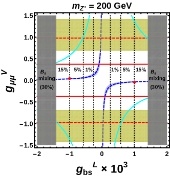
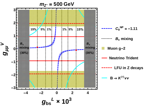
Figure 1: Constraints on the vector $Z^{\prime}\mu\mu$ coupling $g^{V}_{\mu\mu}=g^{L}_{\mu\mu}=g^{R}_{\mu\mu}$ vs. the LH $Z^{\prime}bs$ coupling $g^{L}_{bs}$ (in units of $10^{-3}$) in scenario (i), for $m_{Z^{\prime}}=200$ GeV [left] and $500$ GeV [right]. The red dots show the benchmark points discussed in Section IV. See the main text for details.

Before embarking on this detailed description, we note that, as seen in Fig. 1, the limits on $g^{V}_{\mu\mu}$ are much weaker than those on $g^{L}_{bs}$. Therefore, the $Z^{\prime}$ is likely to decay primarily to leptons, so that its decays into quarks can be ignored. The leptonic-decay dominance simplifies the discussion. In fact, it is also essential for direct observation of the $Z^{\prime}$ at LHC, since searches with $Z^{\prime}\to b\bar{b},b\bar{s}$ suffer from overwhelming QCD background. Thus, in the scenario (i), where $g_{\mu\mu}^{L}=g_{\mu\mu}^{R}\neq 0$, the dominant branching ratios are

$$\mathcal{B}(Z^{\prime}\to\mu^{+}\mu^{-})\simeq\frac{2}{3},\mathcal{B}(Z^{\prime}\to\nu_{\mu}\bar{\nu}_{\mu})\simeq\frac{1}{3}~{}.$$ (7)

In scenario (ii), each of these branching ratios is 50%.

To incorporate the results of $b\to s\ell\ell$ global fits, we use Eq. (3) to convert the $2\sigma$ constraints of Eq. (5) to the space of $g^{L}_{bs}$ vs. $g^{V}_{\mu\mu}$. The result is given by the blue hyperbolae in Fig. 1

As an example of the impact of the choice of scenario among those listed in Sec. II, we note that in scenario (i’), the resulting values of $g^{V}_{\mu\mu}$ are generically higher than those shown in Fig. 1, and have a wider range. Although this somewhat changes the $Z^{\prime}\to\mu^{+}\mu^{-}$ branching ratio, Eq. (7) is still satisfied. Therefore, the results we obtain in Section IV are not affected.

The most important constraint on the $Z^{\prime}bs$ coupling comes from the $B_{s}$ mixing. With the tree-level $Z^{\prime}$ exchange contribution, the total $B_{s}-\bar{B}_{s}$ mixing amplitude relative to the SM one (see, e.g. Ref. Lenz:2010gu ) is given by

$$\frac{M_{12}}{M_{12}^{\text{SM}}}=1+\frac{\left({g^{L}_{bs}}\right)^{2}}{m_{Z^{\prime}}^{2}}\left(\frac{g^{2}_{2}}{16\pi^{2}v^{2}}(V_{tb}V_{ts}^{*})^{2}S_{0}\right)^{-1},$$ (8)

where $S_{0}\simeq 2.3$ is an Inami-Lim function, $g_{2}$ is the SU(2)_L gauge coupling, $v\simeq 246$ GeV, and a common QCD correction factor is assumed for the SM and NP contributions. The mass difference $\Delta m_{B_{s}^{0}}=2|M_{12}|$ is precisely measured, at the per mill level Olive:2016xmw , while the calculation of $M_{12}$ suffers from various sources of uncertainty. One of the dominant uncertainties is the CKM factor, with an uncertainty of $\sim 5$% Charles:2015gya ; Bona:2006sa . The other is the hadronic matrix element, obtained from the lattice. The average of $N_{f}=2+1$ lattice results compiled by FLAG in 2016 Aoki:2016frl implied a $\sim 12$% uncertainty in $M_{12}^{\rm SM}$. Recently, the situation was greatly improved with the advent of the accurate estimate by the Fermilab Lattice and MILC collaborations Bazavov:2016nty , which pushes down the uncertainty of the FLAG average to $\sim 6$%. (See December 2017 update on the FLAG website Aoki:2016frl .) A global analysis of the CKM parameters by CKMfitter Charles:2015gya , published before the recent lattice result Bazavov:2016nty , gives a constraint on $M_{12}$ with NP as $|M_{12}/M_{12}^{\rm SM}|=1.05^{+0.14}_{-0.13}$. On the other hand, the Summer 2016 result Bona:2006sa by UTfit, which includes the result of Ref. Bazavov:2016nty , constrains NP with a better precision: $|M_{12}/M_{12}^{\rm SM}|=1.070\pm 0.088$. As we assume $g^{L}_{bs}$ to be real, the $Z^{\prime}$ contribution always enhances $|M_{12}|$. If one takes these uncertainties to be Gaussian, these results imply $|M_{12}/M_{12}^{\rm SM}|<1.32$ Charles:2015gya or $1.25$ Bona:2006sa at $2\sigma$ for the CKMfitter and UTfit results, respectively. In this paper, we explore NP contributions to $|M_{12}/M_{12}^{\rm SM}|$ at the level of up to $30\%$. Excluding larger contributions leads to the gray-shaded regions in Fig. 1. Future improvements in lattice calculations and measurements of the CKM parameters would tighten the constraint Bona-ICHEP2016 . In Fig. 1, we illustrate the impact of possible future improvements by the vertical dotted lines for deviation of $M_{12}$ from SM by 15% or 5%.

We note that while the CKMfitter Charles:2015gya and UTfit Bona:2006sa results are tolerant to a NP contribution that enhances $|M_{12}|$, there are studies that find the SM prediction of $\Delta m_{B_{s}^{0}}=2|M_{12}|$ to be larger than the measured value, slightly favoring NP that reduces $|M_{12}|$. In particular, a recent study DiLuzio:2017fdq , which adopts the 2017 FLAG result Aoki:2016frl , finds the SM prediction to be $1.8\sigma$ above the measured value. Their result can be read as $|M_{12}/M_{12}^{\rm SM}|\simeq 0.89\pm 0.06$, which allows an enhancement by NP only up to $\sim 1$% at 2$\sigma$. The rather small uncertainty is in part due to a smaller uncertainty of 2.1% assigned to the CKM factor. Addressing the discrepancy among the theoretical calculations is beyond the scope of this paper. Instead, the 1% vertical dotted lines are also shown in Fig. 1 for illustrating the impact of the result by Ref. DiLuzio:2017fdq .

The nonzero LH $Z^{\prime}\mu\mu$ coupling implies also the existence of a $Z^{\prime}\nu\nu$ coupling, due to SU(2)_L. Therefore, constraints are also set by $B\to K^{(*)}\nu\bar{\nu}$. The effective Hamiltonian for $b\to s\nu\bar{\nu}$ is Buras:2014fpa

$$\mathcal{H}_{eff}^{\nu}=\mathcal{N}\sum_{\ell=e,\mu,\tau}C_{L}^{\ell}\left(\bar{s}\gamma^{\alpha}P_{L}b\right)\left[\bar{\nu}_{\ell}\gamma_{\alpha}(1-\gamma_{5})\nu_{\ell}\right]+{\rm h.c.},$$ (9)

where $C_{L}^{\mu}=C_{L}^{\rm SM}+C_{L}^{\rm NP}$ and $C_{L}^{\ell}=C_{L}^{\rm SM}$ ($\ell=e,\tau$) are lepton-flavor dependent Wilson coefficients. The SM contribution is lepton-flavor universal and is given by $C_{L}^{\rm SM}=-X_{t}/s_{W}^{2}$ with $X_{t}=1.469\pm 0.017$ Brod:2010hi . The $Z^{\prime}$ contribution is given by

$$C_{L}^{\rm NP}=\frac{g^{L}_{bs}~{}g^{L}_{\mu\mu}}{2\mathcal{N}m_{Z^{\prime}}^{2}}.$$ (10)

Normalizing $B\to K^{(*)}\nu\bar{\nu}$ branching ratios by the SM ones and defining $\mathcal{R}_{K^{(*)}}^{\nu}\equiv\mathcal{B}(B\to K^{(*)}\nu\bar{\nu})/\mathcal{B}(B\to K^{(*)}\nu\bar{\nu})_{\rm SM}$, we obtain

$$\mathcal{R}_{K}^{\nu}=\mathcal{R}_{K^{*}}^{\nu}=\frac{2}{3}+\frac{1}{3}\left|\frac{C_{L}^{\rm SM}+C_{L}^{\rm NP}}{C_{L}^{\rm SM}}\right|^{2}.$$ (11)

Combining the charged and neutral $B$ meson decays, the tightest limits Amhis:2016xyh are set by Belle Grygier:2017tzo , who find

$$\mathcal{R}_{K}^{\nu}<3.9,\quad\mathcal{R}_{K^{*}}^{\nu}<2.7$$ (12)

at the 90% confidence level (C.L.). The tighter constraint comes from $\mathcal{R}_{K^{*}}^{\nu}$, and is shown by the cyan lines in Fig. 1. The allowed region fully contains the blue hyperbolae favored by $b\to s\ell\ell$

The $Z^{\prime}bs$ and $Z^{\prime}bb$ couplings induce $Z^{\prime}$ production at LHC via $b\bar{s}\to Z^{\prime}$ and $b\bar{b}\to Z^{\prime}$. Hence, with $Z^{\prime}\to\mu^{+}\mu^{-}$, these couplings are constrained by dimuon resonance searches at LHC.

We use the results from ATLAS, performed with 36.1 fb^-1 at 13 TeV Aaboud:2017buh and extract extrac the 95% credibility level limit: $\sigma(pp\to Z^{\prime}+X)\mathcal{B}(Z^{\prime}\to\mu^{+}\mu^{-})<42$ fb (9 fb) for $m_{Z^{\prime}}=200$ GeV (500 GeV). We calculate the $Z^{\prime}$ production cross section at leading order (LO) using MadGraph5_aMC@NLO Alwall:2014hca with the NN23LO1 parton distribution function (PDF) set Ball:2013hta . As the ATLAS search does not veto additional activity in the event, we include also the processes $gs\to Z^{\prime}b$, $gb\to Z^{\prime}b$ and $gg\to Z^{\prime}b\bar{b},Z^{\prime}b\bar{s}$ in the cross-section calculation. We defer the more detailed discussion about $Z^{\prime}$ production at LHC to Section IV. From the cross sections and the ATLAS limits, we find

$$\sqrt{|g^{L}_{bs}|^{2}+0.33|g^{L}_{bb}|^{2}}<0.004\quad(m_{Z^{\prime}}=200~{}{\rm GeV}),$$

$$\sqrt{|g^{L}_{bs}|^{2}+0.21|g^{L}_{bb}|^{2}}<0.011\quad(m_{Z^{\prime}}=500~{}{\rm GeV})$$ (13)

in scenario (i). In scenario (ii), where the $Z^{\prime}$ couples to the LH muon current, the limits are weakened by an overall factor of $2/\sqrt{3}$ on the right-hand side due to the change in $\mathcal{B}(Z^{\prime}\to\mu^{+}\mu^{-})$.

As long as $|g^{L}_{bb}|\lesssim|g^{L}_{bs}|$, which is our scenario of interest, these limits are significantly weaker than those from the $B_{s}-\bar{B}_{s}$ mixing. Hence, they are not shown in Fig. 1. For flavor universal models, $Z^{\prime}$ masses below $m_{Z^{\prime}}\lesssim 3-4.5$ TeV are ruled out by Ref. Aaboud:2017buh with 95% CL. However, a very weakly coupled and flavor non-universal light $Z^{\prime}$ such as described by Eq.(1), escapes the detection and could emerge in the future runs of LHC.

Muon pair production in the scattering of a muon neutrino and a nucleus $N$, known as neutrino trident production, tightly constrains $Z^{\prime}\mu\mu$ and $Z^{\prime}\nu_{\mu}\nu_{\mu}$ couplings Altmannshofer:2014pba . The ratio between the total $\nu_{\mu}N\to\nu_{\mu}N\mu^{+}\mu^{-}$ cross section and its SM prediction is given by Altmannshofer:2014cfa

$$\frac{\sigma}{\sigma^{\rm SM}}=\frac{1+\left[1+4s_{W}^{2}+2(g_{\mu\mu}^{V})^{2}\frac{v^{2}}{m_{Z^{\prime}}^{2}}\right]^{2}}{1+(1+4s^{2}_{W})^{2}},$$ (14)

in scenario (i) with $m_{Z^{\prime}}\gtrsim 10$ GeV. The measurement Mishra:1991bv by the CCFR collaboration is in a good agreement with SM, and implies $\sigma/\sigma^{\rm SM}=0.82\pm 0.28$. We show the resulting $2\sigma$ upper limits on $|g^{V}_{\mu\mu}|$ by the horizontal solid red lines in Fig. 1.

The couplings of the $Z$ boson with the muon and muon neutrino are modified by $Z^{\prime}$-loop contributions, which can lead to violation of the lepton-flavor universality in $Z$ decays. In scenario (i), the vector and axial-vector $Z\mu\mu$ couplings relative to the SM-like $Zee$ couplings are given by Altmannshofer:2014cfa ; Altmannshofer:2016brv

$$\frac{g_{V\mu}}{g_{Ve}}\simeq\frac{g_{A\mu}}{g_{Ae}}\simeq 1+\frac{(g^{V}_{\mu\mu})^{2}}{16\pi^{2}}{\rm Re}\left[\mathcal{K}(m_{Z}^{2}/m_{Z^{\prime}}^{2})\right],$$ (15)

where $\mathcal{K}(m_{Z}^{2}/m_{Z^{\prime}}^{2})$ is a loop function given in Ref. Haisch:2011up , and its real part is taken to match the convention of Ref. ALEPH:2005ab . Here, the lepton-flavor universality in the SM case is exploited. Similarly, normalized $Z\nu\nu$ couplings are given by

$$\frac{g_{V\nu}}{g_{Ae}}=\frac{g_{A\nu}}{g_{Ae}}\simeq-\left\{1+\frac{1}{3}\frac{(g^{L}_{\mu\mu})^{2}}{16\pi^{2}}{\rm Re}\left[\mathcal{K}(m_{Z}^{2}/m_{Z^{\prime}}^{2})\right]\right\},$$ (16)

where the factor of $1/3$ effectively takes into account the fact that only $Z\to\nu_{\mu}\bar{\nu}_{\mu}$ is affected by the $Z^{\prime}$ among the three neutrino modes.

The $Z$ couplings were very precisely measured at SLC and LEP. Relevant results from the average of 14 electroweak measurements are $g_{Ve}=-0.03816\pm 0.00047$, $g_{Ae}=-0.50111\pm 0.00035$, $g_{V\mu}=-0.0367\pm 0.0023$, $g_{A\mu}=-0.50120\pm 0.00054$ and $g_{V\nu}=g_{A\nu}=0.5003\pm 0.0012$ ALEPH:2005ab . Of the four possible $Z$ coupling ratios, we take only the one which is most sensitive to the effect of the $Z^{\prime}$, i.e. $g_{A\mu}/g_{Ae}=1.00018\pm 0.00128$, where the uncertainties are added in quadrature. The resulting $2\sigma$ upper limits on $|g^{V}_{\mu\mu}|$ are shown by the horizontal red dashed lines in Fig. 1.

Nonzero values of $g_{bs}^{L}$ or $g_{bb}^{L}$ can alter the $Zbb$ and $Zss$ couplings at one loop. Taking the $b$ and $s$ quarks to be massless, we find that the $Z^{\prime}$ loop with a nonzero $g_{bs}^{L}$ modifies the LH $Zbb$ and $Zss$ couplings $g_{Lb}$ and $g_{Ls}$ relative to their SM values $g_{Lb}^{\rm SM}$ and $g_{Ls}^{\rm SM}$ in the same way as the LH $Z\mu\mu$ coupling, but with the replacement $g_{\mu\mu}^{L}\to g_{bs}^{L}$:

$$\frac{g_{Lb}}{g_{Lb}^{\rm{SM}}}\simeq\frac{g_{Ls}}{g_{Ls}^{\rm{SM}}}\simeq 1+\frac{(g^{L}_{bs})^{2}}{16\pi^{2}}{\rm Re}\left[\mathcal{K}(m_{Z}^{2}/m_{Z^{\prime}}^{2})\right].$$ (17)

The RH counterparts remain unchanged. The effect of the $Z^{\prime}$ loop can be constrained by comparing the measured value $g_{Lb}=-0.4182\pm 0.0015$ ($g_{Ls}=-0.423\pm 0.012$) ALEPH:2005ab to the corresponding SM prediction $g_{Lb}^{\rm{SM}}=-0.42114^{+0.00045}_{-0.00024}$ ($g_{Ls}^{\rm{SM}}=-0.42434^{+0.00018}_{-0.00016}$), derived from the SM $Z$-pole fit ALEPH:2005ab . Since $g_{Lb}$ is more precisely measured than $g_{Ls}$, we use $g_{Lb}$ to extract the limit on $g_{bs}^{L}$. Adding the errors in $g_{Lb}$ and $g_{Lb}^{\rm{SM}}$ in quadrature after symmetrizing the $g_{Lb}^{\rm{SM}}$ errors, we find the $2\sigma$ upper limit $|g_{bs}^{L}|\lesssim 0.34~{}(0.67)$ for $m_{Z^{\prime}}=$ 200 (500) GeV. These limits are much weaker than the ones obtained from the $B_{s}$ mixing, and we do not display them in Fig. 1. A similar conclusion can be made for the $g_{bb}^{L}$ coupling as well.

If both $g_{bs}^{L}$ and $g_{bb}^{L}$ are nonzero, an FCNC decay $Z\to b\bar{s}$, which is absent in the SM at tree-level, is induced by the one-loop $Z^{\prime}$ contribution. A preliminary result by DELPHI Fuster:1999dj sets the 90% CL upper limit $R_{b\ell}=\sum_{q=d,s}\sigma(e^{+}e^{-}\to b\bar{q}+\bar{b}q)/\sigma(e^{+}e^{-}\to{\rm hadrons})\leq 2.6\times 10^{-3}$ at the energy scale of the $Z$ mass. Using $\mathcal{B}(Z\to{\rm hadrons})\simeq 70$% Olive:2016xmw , one may rewrite the limit as $\sum_{q=d,s}\mathcal{B}(Z\to b\bar{q}+\bar{b}q)\lesssim 1.8\times 10^{-3}$. Since the $Z^{\prime}$-loop-induced LH $Zbs$ coupling is suppressed by the factor $g_{bs}^{L}g_{bb}^{L}/(16\pi^{2})$, the DELPHI limit is relevant only if both $g_{bs}^{L}$ and $g_{bb}^{L}$ are $\mathcal{O}(1)$ and the $Z^{\prime}$ mass is not far from the $Z$ mass. Since the $B_{s}$-mixing constraint on $g_{bs}^{L}$ is much tighter, and we concentrate on the case $|g_{bb}^{L}|\lesssim|g_{bs}^{L}|$, the impact on $\mathcal{B}(Z\to b\bar{s}+\bar{b}s)$ is generically far below the DELPHI limit in the scenarios considered in this paper.

The $Z^{\prime}$ one-loop contribution to the muon anomalous magnetic moment $a_{\mu}=(g_{\mu}-2)/2$ is Pospelov:2008zw

$$\Delta a_{\mu}=\frac{(g^{V}_{\mu\mu})^{2}}{12\pi^{2}}\frac{m_{\mu}^{2}}{m_{Z^{\prime}}^{2}},$$ (18)

where scenario (i) and $m_{Z^{\prime}}\gg m_{\mu}$ are assumed. The difference between the measured value of $a_{\mu}$ and its SM prediction is $(2.9\pm 0.9)\times 10^{-9}$ Jegerlehner:2009ry . Assigning this difference to Eq. (18) yields the dark yellow $2\sigma$ regions in Fig. 1. Since the $2\sigma$ constraints from the neutrino trident cross section are tighter, the $Z^{\prime}$ does not solve the tension in the muon $g-2$. At the $3\sigma$ level, the $g_{\mu}-2$ regions become compatible with the neutrino trident production constraints. Therefore, we ignore $g_{\mu}-2$ in the rest of this paper.

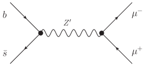
Figure 2: A Feynman diagram for the process $b\bar{s}\to Z^{\prime}\to\mu^{+}\mu^{-}$.

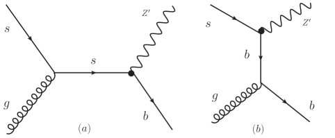
Figure 3: Feynman diagrams for $gs\to Z^{\prime}b$.

We have discussed so far the constraints in scenario (i), summarized in Fig. 1 on the $g^{V}_{\mu\mu}$ vs. $g^{L}_{bs}$ plane. From Fig. 1, we find the constraint on $g^{L}_{bs}$ is very stringent due to the $B_{s}-\bar{B}_{s}$ mixing, while the constraint on $g^{V}_{\mu\mu}$ is much weaker. With the 30% NP effects allowed in the $B_{s}-\bar{B}_{s}$ mixing amplitude, the former constraint is $|g_{bs}^{L}|\lesssim 1.4~{}(3.6)\times 10^{-3}$ for $m_{Z^{\prime}}=200~{}(500)$ GeV, imposing the lower limit on the $Z^{\prime}\mu\mu$ coupling $|g^{V}_{\mu\mu}|\gtrsim 0.031~{}(0.078)$ on the $b\to s\ell\ell$ hyperbolae. This validates the numerical values of the branching ratios in Eq. (7) to a good approximation, if $|g_{bb}^{L}|$ is not too large compared to $|g_{bs}^{L}|$.

The qualitative feature is the same in scenario (ii), where the $Z^{\prime}\mu\mu$ coupling is of LH, as the $B_{s}-\bar{B}_{s}$ mixing constraint does not change. Some of the other observables would give slightly different constraints on the $Z^{\prime}\mu\mu$ coupling, but the effect is minor to our study. The only notable difference from scenario (i) is the slight change in the value of $\mathcal{B}(Z^{\prime}\to\mu^{+}\mu^{-})$ from Eq. (7). A nonzero axial-vector $Z^{\prime}\mu\mu$ coupling can make $B_{s}\to\mu^{+}\mu^{-}$ relevant, but the latest LHCb result Aaij:2017vad does not exclude the allowed regions for the $b\to s\ell\ell$ anomalies.

IV Discovery and identification of the $Z^{\prime}$ at LHC

Having determined the constraints on the $Z^{\prime}$ couplings, we proceed to study signatures for direct production of the on-shell $Z^{\prime}$ in $pp$ collisions with a center-of-mass energy of $\sqrt{s}=14$ TeV. The goal of this study is to ascertain the LHC potential for both discovery of the $Z^{\prime}$ and determination of the flavor structure of its couplings. Therefore, motivated by the tensions in $b\to s\ell\ell$, we focus on the role of the $Z^{\prime}bs$ coupling $g^{L}_{bs}$. If this is the dominant coupling to the quark sector, the $Z^{\prime}$ will be primarily produced via the parton-level process $b\bar{s}\to Z^{\prime}$ shown in Fig. 2. With the decay $Z^{\prime}\to\mu^{+}\mu^{-}$, the $Z^{\prime}$ may be discovered in the conventional dimuon resonance searches.

Such a discovery of a dimuon resonance, however, does not necessarily imply the existence of the $Z^{\prime}bs$ coupling. In general, the process $pp\to Z^{\prime}+X$ may be facilitated by coupling to other quarks, particularly flavor-diagonal couplings. To test for dominance of the $Z^{\prime}bs$ coupling, we propose to also search for $pp\to Z^{\prime}b+X$ (see Fig. 3 for typical parton-level processes). A $Z^{\prime}bb$ coupling, predicted in many models (e.g., Refs Ko:2017quv ; Bonilla:2017lsq ; Alonso:2017uky ; Altmannshofer:2014cfa ), motivated by the $b\to s\ell\ell$ anomalies, also contribute to $pp\to Z^{\prime}+X$ and $pp\to Z^{\prime}b+X$ via the parton level processes $b\bar{b}\to Z^{\prime}$ and $gb\to Z^{\prime}b$. Since a $Z^{\prime}bb$ coupling also leads to $pp\to b\bar{b}Z^{\prime}+X$, via, for example, $gg\to Z^{\prime}b\bar{b}$, measuring the cross section for $pp\to Z^{\prime}b\bar{b}+X$ may facilitate to discriminate the $Z^{\prime}bb$ coupling from $Z^{\prime}bs$. Similarly, the production process $pp\to Z^{\prime}b\bar{s}+X$, occurring due to $gg\to Z^{\prime}b\bar{s}$, can in principle help probe the $Z^{\prime}bs$ coupling.

We explore these signatures using the effective Lagrangian of Eq. (1) with scenario (i), i.e., with a vector $Z^{\prime}\mu\mu$ coupling. For each of the two $Z^{\prime}$ mass values studied, we fix the couplings to the benchmark points shown by the red dots in Fig. 1:

$$\left|g^{L}_{bs}\right|=0.001,\quad\left|g^{V}_{\mu\mu}\right|=0.04\quad(m_{Z^{\prime}}=200~{}{\rm GeV}),$$

$$\left|g^{L}_{bs}\right|=0.0025,\quad\left|g^{V}_{\mu\mu}\right|=0.1\quad(m_{Z^{\prime}}=500~{}{\rm GeV}).$$ (19)

These values are selected such that $g^{L}_{bs}$ leads to a 15% enhancement in the $B_{s}-\bar{B}_{s}$-mixing amplitude $M_{12}$. The value of $g^{V}_{\mu\mu}$ is then chosen so as to lie in the range given by Eqs. (5) and (3). We note that one may take a larger $|g^{L}_{bs}|$ (with a smaller $|g^{V}_{\mu\mu}|$), which would enlarge the $pp\to Z^{\prime}+X$ and $pp\to Z^{\prime}b+X$ cross sections by up to a factor of two, with the $B_{s}-\bar{B}_{s}$-mixing constraint saturated at $2\sigma$, i.e. a $\sim$30% enhancement in $M_{12}$.

For the $Z^{\prime}bb$ coupling, we study three cases for each benchmark point. The baseline case is $g^{L}_{bb}=0$, which restricts assumptions about the $Z^{\prime}$ couplings to the minimum needed to explain the $b\to s\ell\ell$ anomalies. In addition, we also explore the cases $g^{L}_{bb}=g^{L}_{bs}$ and $g^{L}_{bb}=2g^{L}_{bs}$, to study the impact of a nonzero $g^{L}_{bb}$. These choices of quark couplings satisfy the dimuon resonance search limits in Eq. (13) and maintain the $Z^{\prime}$ branching ratios in Eq. (7).

$m_{Z^{\prime}}$ (GeV)	$\sigma_{\rm signal}$ (fb)			$\sigma_{\rm background}$ (fb)
	$g^{L}_{bb}=0$	$g^{L}_{bb}=g^{L}_{bs}$	$g^{L}_{bb}=2g^{L}_{bs}$	DY	$t\bar{t}$	$Wt$	$VV$
200	1.0	1.3	2.2	170	41	4.1	5.1
500	0.27	0.33	0.50	14	4.3	0.5	1.0

Table 1: Cross sections for the signal process $pp\to Z^{\prime}+X$ with $Z^{\prime}\to\mu^{+}\mu^{-}$, and the dominant backgrounds after the event selection for the benchmark points defined in Eq. (19) with the three choices for $g_{bb}^{L}$. The combined cross sections for $WW$, $WZ$ and $ZZ$ backgrounds are denoted together as $VV$.

$m_{Z^{\prime}}$ (GeV)	Local significance
	$g^{L}_{bb}=0$	$g^{L}_{bb}=g^{L}_{bs}$	$g^{L}_{bb}=2g^{L}_{bs}$
200	3.7	4.9	8.3
500	3.3	4.1	6.5

Table 2: Local significance $S_{l}=N_{S}/\sqrt{N_{B}}$ for discovery of the process $pp\to Z^{\prime}+X$ with $Z^{\prime}\to\mu^{+}\mu^{-}$, with an integrated luminosity of $3000~{}{\rm fb}^{-1}$, given the signal and background cross sections shown in Table 1.

In the following subsections, we mainly focus on the discovery potential of the $Z^{\prime}$ in the production processes $pp\to Z^{\prime}+X$, $pp\to Z^{\prime}b+X$, and $pp\to Z^{\prime}b\bar{b}+X$, with the $Z^{\prime}$ always decaying to $\mu^{+}\mu^{-}$. We use Monte Carlo event generator MadGraph5_aMC@NLO Alwall:2014hca to generate signal and background samples at LO with the NN23LO1 PDF set Ball:2013hta . The effective Lagrangian of Eq. (1) is implemented in the FeynRules 2.0 Alloul:2013bka framework. The matrix elements for signal and background are generated with up to two additional jets and interfaced with PYTHIA 6.4 Sjostrand:2006za for parton showering and hadronization. Matching is performed with the MLM prescription Alwall:2007fs . The generated events are passed into the Delphes 3.3.3 deFavereau:2013fsa fast detector simulation to incorporate detector effects based on ATLAS.

IV.1 Observation of $pp\to Z^{\prime}+X$

Several SM processes constitute background for $pp\to Z^{\prime}+X$, where we remind the reader that the $Z^{\prime}$ decays into $\mu^{+}\mu^{-}$. The dominant background is due to the Drell-Yan (DY) events, $pp\to Z/\gamma^{*}+X$. The $pp\to t\bar{t}$ events with semileptonic decay of both top quarks is the next largest background. Smaller backgrounds arise from $pp\to Wt$ and $VV$, where $V\equiv W,Z$. Background may also arise from leptons produced in heavy-flavor decays or from jets faking leptons. These background sources are not well modeled by the simulation tools, and we ignore them, assuming that they can be reduced to subdominant level with lepton quality cuts without drastically impacting the results of our analysis.

We scale the LO cross sections obtained by MadGraph5_aMC@NLO as follows. The DY cross section is normalized to a NNLO QCD+NLO EW cross section by a factor of $1.27$, obtained with FEWZ 3.1 Li:2012wna in the dimuon-invariant mass range $m_{\mu\mu}>106$ GeV. We normalize the LO $pp\to t\bar{t}$ and $pp\to Wt$ cross sections to NNLO+NNLL cross sections by $1.84$ twiki and $1.35$ Kidonakis:2010ux , respectively. The $pp\to WW$, $pp\to WZ$ and $pp\to ZZ$ cross sections are normalized to NNLO QCD by $1.98$ Gehrmann:2014fva , $2.07$ Grazzini:2016swo and $1.74$ Cascioli:2014yka , respectively. We do not apply correction factors to the signal cross sections throughout this paper.

$m_{Z^{\prime}}$ (GeV)	$\sigma_{\rm signal}$ (fb)			$\sigma_{\rm background}$ (fb)
	$g^{L}_{bb}=0$	$g^{L}_{bb}=g^{L}_{bs}$	$g^{L}_{bb}=2g^{L}_{bs}$	${\rm DY}+b$	${\rm DY}+c$	${\rm DY}+j$	$t\bar{t}$	$Wt$	$VV$
200	0.17	0.22	0.37	1.3	1.0	0.22	5.6	0.8	0.5
500	0.043	0.049	0.10	0.15	0.048	0.028	0.26	0.08	0.064

Table 3: Cross sections for the signal process $pp\to Z^{\prime}b+X$ with $Z^{\prime}\to\mu^{+}\mu^{-}$, and the dominant backgrounds after the event selection for the benchmark points defined in Eq. (19) with the three choices for $g_{bb}^{L}$.

We select events that contain at least two oppositely charged muons. The transverse momentum of each muon is required to satisfy $p^{T}_{\mu}>50$ GeV, and its pseudorapidity must be in the range $|\eta_{\mu}|<2.5$. The two muons must satisfy $\Delta R_{\mu\mu}=\sqrt{\Delta\phi^{2}_{\mu\mu}+\Delta\eta^{2}_{\mu\mu}}>0.4$, where $\Delta\phi_{\mu\mu}$ and $\Delta\eta_{\mu\mu}$ are the separations in azimuthal angle and pseudorapidity between the muons. Finally, we require the invariant mass of the two muons to satisfy $|m_{\mu\mu}-m_{Z^{\prime}}|<m_{\rm cut}$, where $m_{\rm cut}=4$ GeV and 16 GeV for $m_{Z^{\prime}}=200$ GeV and $m_{Z^{\prime}}=500$ GeV, respectively. These values are chosen so as to maximize the naive local significance of the no-signal hypothesis, $S_{l}=N_{S}/\sqrt{N_{B}}$, where $N_{S}$ and $N_{B}$ are the expected signal and background yields.

The invariant mass cut $|m_{\mu\mu}-m_{Z^{\prime}}|<m_{\rm cut}$ is not realistic for a discovery scenario, in which one does not know the true mass $m_{Z^{\prime}}$. However, the value of $S_{l}$ thus obtained is a rough estimate of the one that will be found by the more sophisticated analysis that will eventually be performed with the full LHC data. One is actually interested in the global significance $S_{g}$, which accounts for the probability to obtain the given value of $S_{l}$ anywhere in the dimuon-invariant mass range. Rigorous methods for estimating $S_{g}$ exist Cowan:2010js . However, at this level of approximation, it is sufficient to use the crude estimate

$$P_{g}=P_{l}{m_{\rm cut}\over m_{\rm range}},$$ (20)

where $P_{g}$ and $P_{l}$ are the $\chi^{2}$ probabilities corresponding to $S_{g}$ and $S_{l}$, respectively, and $m_{\rm range}$ is the size of the range of $m_{\mu\mu}$ values explored in the analysis. Since cross sections drop to negligible levels at high $m_{\mu\mu}$, it is reasonable to take $m_{\mu\mu}\sim 2$–$3$ TeV for this estimate.

The cross sections for signal and backgrounds after the cuts are listed in Table 1 for the benchmark points defined in Eq. (19) with the three choices of $g_{bb}^{L}$. The corresponding values of the local significance $S_{l}$ for an integrated luminosity $L=3000~{}{\rm fb}^{-1}$ are summarized in Table 2. Inserting the values of $S_{l}$ into Eq. (20), we conclude that the global significance will likely be greater than $5\sigma$ for the case $g^{L}_{bb}=2g^{L}_{bs}$, allowing separate discovery by ATLAS and CMS. For $|g^{L}_{bb}|\leq|g^{L}_{bs}|$, the global significance will be under $5\sigma$. Whether the $5\sigma$ mark will be passed by combining ATLAS and CMS results is beyond the precision of our rough estimate.

A larger $|g_{bs}^{L}|$ can enhance the significance in each benchmark scenario. For the scenario of $m_{Z^{\prime}}=200~{}(500)$ GeV with $g_{bb}^{L}=0$, taking $|g_{bs}^{L}|=0.0013~{}(0.0034)$ with $|g_{\mu\mu}^{V}|=0.031~{}(0.074)$ pushes the local significance slightly above $6\sigma$, which may imply a global significance of $5\sigma$. In this case, the $B_{s}-\bar{B}_{s}$ mixing amplitude $|M_{12}|$ is also enhanced from the SM one by 25% (28%), but still within the nominal 2$\sigma$ allowed range, as discussed in Sec. III.

IV.2 Observation of $pp\to Z^{\prime}b+X$

$m_{Z^{\prime}}$ (GeV)	Local significance
	$g^{L}_{bb}=0$	$g^{L}_{bb}=g^{L}_{bs}$	$g^{L}_{bb}=2g^{L}_{bs}$
200	3.0	3.9	6.6
500	3.0	3.4	7.2

Table 4: Local significance $S_{l}=N_{S}/\sqrt{N_{B}}$ for discovery of the process $pp\to Z^{\prime}b+X$ with $Z^{\prime}\to\mu^{+}\mu^{-}$, with an integrated luminosity of $3000~{}{\rm fb}^{-1}$, given the signal and background cross sections shown in Table 3.

The main SM background for $pp\to Z^{\prime}b+X$ is $pp\to t\bar{t}$. The second-largest background is Drell-Yan with at least one additional $b$ jet, labeled as ${\rm DY}+b$. Smaller contributions arise from ${\rm DY}+c$, $pp\to Wt$, $pp\to VV$, and ${\rm DY}+j$, where $j$ stands for a jet from a gluon or a $u$, $d$, or $s$ quark. We normalize the cross sections for ${\rm DY}+b$, ${\rm DY}+c$, and ${\rm DY}+j$ to NNLO QCD by $1.83$ Boughezal:2016isb . The correction factors for $pp\to t\bar{t}$, $pp\to Wt$, and $pp\to VV$ are taken to be the same as in Section IV.1.

We select simulated events that contain at least two opposite-charge muons. The muons are required to be in the pseudorapidity range $|\eta_{\mu}|<2.5$, have minimal transverse momenta of $p^{T}_{\mu}>50~{}(60)$ GeV for $m_{Z^{\prime}}=200~{}(500)$ GeV, and be separated by $\Delta R_{\mu\mu}>0.4$. Jets are reconstructed using the anti-$k_{T}$ algorithm with radius parameter $R=0.5$. It is assumed that a $b$-tagging algorithm reduces the efficiency for $c$ jets and light jets by factors of 5 and 137, respectively ATLAS:2014ffa . Its efficiency for $b$ jets is calculated in Delphes, accounting for the $p_{T}$ and $\eta$ dependence. The leading $b$ jet is required to have transverse momentum $p^{T}_{b}>30$ GeV with $|\eta_{b}|<2.5$, and its separation from each of the two leading muons must satisfy $\Delta R_{b\mu}>0.4$. We reject events that have a second $b$-tagged jet with $p^{T}_{b}>30$ GeV, slightly increasing the local significance. The missing transverse energy must be less than $40$ GeV, in order to reduce $pp\to t\bar{t}$ and $pp\to Wt$ backgrounds. Finally, we apply the optimized dimuon-invariant mass cut $|m_{\mu\mu}-m_{Z^{\prime}}|<5~{}(15)$ GeV for $m_{Z^{\prime}}=200~{}(500)$ GeV.

The resulting cross sections are shown in Table 3, and the corresponding local signal significances with 3000 fb^-1 are summarized in Table 4. The local significances are slightly smaller than the corresponding ones in Table 2, except in the case of $m_{Z^{\prime}}=500$ GeV and $g_{bb}=2g_{bs}^{L}$. Thus, we conclude that, like $pp\to Z^{\prime}+X$, the process $pp\to Z^{\prime}b+X$ is likely be discovered at $S_{g}>5$ if $g_{bb}^{L}\geq 2g_{bs}^{L}$ in our benchmark points. By scaling the values in Table 4, we observe that a local significance of $6\sigma$ can be attained with $|g_{bs}^{L}|\gtrsim 0.0014~{}(0.0036)$ for $m_{Z^{\prime}}=200~{}(500)$ GeV, even if $g_{bb}^{L}=0$, at the cost of a $\sim 30$% enhancement in $|M_{12}/M_{12}^{\rm SM}|$.

IV.3 Observation of $pp\to Z^{\prime}b\bar{b}+X$ and $pp\to Z^{\prime}b\bar{s}+X$

$m_{Z^{\prime}}$ (GeV)	$\sigma_{\rm signal}$ (fb)			$\sigma_{\rm background}$ (fb)
	$g^{L}_{bb}=0$	$g^{L}_{bb}=g^{L}_{bs}$	$g^{L}_{bb}=2g^{L}_{bs}$	${\rm DY}+\mbox{h.f.}$ jets	$t\bar{t}$	$Wt$
200	0.00018	0.0025	0.0094	0.2	1.5	0.5
500	0.00008	0.0006	0.0026	0.07	0.27	0.17

Table 5: Cross sections for the signal process $pp\to Z^{\prime}b\bar{b}+X$ with $Z^{\prime}\to\mu^{+}\mu^{-}$, and the dominant backgrounds after the event selection for the benchmark points defined in Eq. (19) with the three choices for $g_{bb}^{L}$.

$m_{Z^{\prime}}$ (GeV)	Local significance
	$g^{L}_{bb}=0$	$g^{L}_{bb}=g^{L}_{bs}$	$g^{L}_{bb}=2g^{L}_{bs}$
200	0.007	0.1	0.35
500	0.006	0.05	0.2

Table 6: Local significance $S_{l}=N_{S}/\sqrt{N_{B}}$ for discovery of the process $pp\to Z^{\prime}b\bar{b}+X$ with $Z^{\prime}\to\mu^{+}\mu^{-}$, with an integrated luminosity of $3000~{}{\rm fb}^{-1}$, given the signal and background cross sections shown in Table 5.

The dominant SM backgrounds for $pp\to Z^{\prime}b\bar{b}+X$ are $pp\to t\bar{t}$, $pp\to Wt$ and ${\rm DY}+b$ or $c$ jets. $pp\to VV$ gives a negligible contribution. We adopt the same correction factors for the background cross sections and follow the same event selection criteria as in Section IV.3, and in addition require the subleading $b$ jet to have $p^{T}_{b}>30$ GeV, $|\eta_{b}|<2.5$, and to be separated from the leading $b$ jet and each of the two leading muons by $\Delta R>0.4$, for both the $Z^{\prime}$ masses.

The resulting cross sections are shown in Table 5. The $g^{L}_{bb}=0$ cases have tiny but nonzero cross sections, due to production via $b\bar{s}\to Z^{\prime}g^{*}$, with $g^{*}\to b\bar{b}$. By contrast, a nonzero $g^{L}_{bb}$ induces the less suppressed process $gg\to Z^{\prime}b\bar{b}$. The corresponding local signal significances for 3000 fb^-1 are given in Table 6. As the local significances are much less than 1, we conclude that observation of this process is not possible at LHC within the range of couplings explored here.

In general, $|g_{bb}^{L}|$ may take a larger value, up to the limit of Eq. (13), namely, $|g^{L}_{bb}|=0.007$ ($0.024$) for $m_{Z^{\prime}}=200$ (500) GeV with $g^{L}_{bs}\sim 0$. With these values, we estimate the cross section of $pp\to Z^{\prime}b\bar{b}+X$ to be 0.098 fb (0.055 fb) after the event selection cuts. This corresponds to a local significance of around $3.6\sigma$ ($4.1\sigma$) for an integrated luminosity of $3000~{}{\rm fb}^{-1}$. Thus, a global significance of $5\sigma$ is not likely. We note, however, that since we used the same QCD correction factors for the background cross sections as in the $pp\to Z^{\prime}b+X$ case, there is a greater uncertainty on these cross sections.

Generally, the cross section for $pp\to Z^{\prime}b\bar{b}+X$ is strongly suppressed by the 3-body phase space. Since the same suppression applies for $pp\to Z^{\prime}b\bar{s}+X$, one expects the cross section for this process to be small as well. Moreover, the process $pp\to Z^{\prime}b\bar{s}+X$ would also suffer from light-jet backgrounds which make the discovery not possible, given the $B_{s}-\bar{B}_{s}$ mixing constraint.

V Impact of the right-handed $Z^{\prime}bs$ coupling

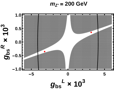
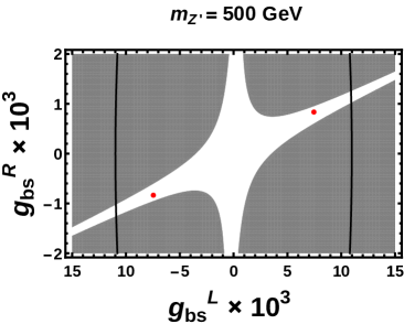
Figure 4: Constraints on $g^{R}_{sb}$ vs. $g^{L}_{sb}$ (in units of $10^{-3}$) for $m_{Z^{\prime}}=200$ GeV [left] and 500 GeV [right], when allowing the $B_{s}-\bar{B}_{s}$-mixing amplitude to deviate by up to 30% from its SM prediction. The gray regions are excluded. The solid lines show the exclusion by the ATLAS dimuon resonance search Aaboud:2017buh for $\mathcal{B}(Z^{\prime}\to\mu^{+}\mu^{-})\simeq 2/3$. The red dots show our benchmark points.

In this section, we study an impact of a tiny but nonzero RH $Z^{\prime}bs$ coupling by adding the following terms to the effective Lagrangian in Eq. (1):

$$\Delta\mathcal{L}=-g^{R}_{bs}\left(\bar{b}\gamma^{\alpha}P_{R}s+\bar{s}\gamma^{\alpha}P_{R}b\right)Z^{\prime}_{\alpha}.$$ (21)

The resulting additional contributions to $b\to s\mu^{+}\mu^{-}$ are described by effective operators as in Eq. (2), with $P_{L}$ replaced by $P_{R}$, and with $C_{9}^{\rm NP}$ and $C_{10}^{\rm NP}$ replaced by the Wilson coefficients

$$C^{\prime}_{9}=\frac{g^{R}_{bs}~{}g^{V}_{\mu\mu}}{\mathcal{N}m_{Z^{\prime}}^{2}},\quad C^{\prime}_{10}=\frac{g^{R}_{bs}~{}g^{A}_{\mu\mu}}{\mathcal{N}m_{Z^{\prime}}^{2}}.$$ (22)

There is no significant indication for nonzero $C^{\prime}_{9,10}$ in the majority of the $b\to s\ell\ell$ global fit analyses. However, even a tiny $g^{R}_{bs}$ can drastically affect the $B_{s}-\bar{B}_{s}$ mixing, which is now given by Altmannshofer:2014cfa

$$\frac{M_{12}}{M_{12}^{\rm SM}}=1+\frac{1}{m_{Z^{\prime}}^{2}}\left[(g^{L}_{bs})^{2}-9.7g^{L}_{bs}g^{R}_{bs}+(g^{R}_{bs})^{2}\right]$$

$$\times\left(\frac{g^{2}_{2}}{16\pi^{2}v^{2}}(V_{tb}V_{ts}^{*})^{2}S_{0}\right)^{-1},$$ (23)

calculated with the hadronic matrix elements in Ref. Buras:2012jb . The large negative coefficient of the $g^{L}_{bs}g^{R}_{bs}$ term, which is partly due to renormalization group effects Buras:2001ra , means that a small value of $g^{R}_{bs}$ allows for a large $g^{L}_{bs}$, due to cancellation between the terms. In Fig. 4 we show the $B_{s}-\bar{B}_{s}$-mixing constraint on $g^{R}_{bs}$ vs. $g^{L}_{bs}$, when $|M_{12}|$ is allowed to change by up to 30% of its SM value. Reducing the allowed NP contribution to $|M_{12}|$, say, to 15%, would narrow the width of the tilted-cross-shaped allowed region in Fig. 4. However, it would not change the conclusion, namely, that a large value of $|g^{L}_{bs}|$ is allowed. What now becomes the most significant limit on $g^{L}_{bs}$ is the ATLAS dimuon resonance search Aaboud:2017buh , shown by the solid lines, assuming Eq. (7).

The cancellation in $M_{12}$ requires $g_{bs}^{L}g_{bs}^{R}>0$. This implies $({\rm Re}~{}C_{9}^{\rm NP})({\rm Re}~{}C^{\prime}_{9})>0$, contrary to the best-fit values for $C_{9}^{\rm NP}$ and $C^{\prime}_{9}$, e.g., Refs. Capdevila:2017bsm ; Altmannshofer:2017yso . However, the cancellation requires only $g_{bs}^{R}\sim 0.1g_{bs}^{L}$ or $C^{\prime}_{9}\sim 0.1C_{9}^{\rm NP}$. While the fits favor $C_{9}^{\rm NP}\sim-1$ and are consistent with $C^{\prime}_{9}=0$, they cannot exclude a small negative $C_{9}^{\prime}$. Indeed, the point $(C_{9}^{\rm NP},C^{\prime}_{9})=(-1.11,-0.1)$ is at the border of the 1$\sigma$ ellipse in Ref. Capdevila:2017bsm with the assumption $C_{10}^{\rm NP}=C^{\prime}_{10}=0$.

To illustrate the impact of such a possibly large $Z^{\prime}bs$ coupling on the $Z^{\prime}$ discovery potential, we consider scenario (i) with the following benchmark points for $m_{Z^{\prime}}=200$ and $500$ GeV respectively (corresponding to the dots in Fig. 4):

$$\left|g^{L}_{bs}\right|=0.0032,\left|g^{R}_{bs}\right|=0.00036,\left|g^{V}_{\mu\mu}\right|=0.012,$$

$$\left|g^{L}_{bs}\right|=0.0075,\left|g^{R}_{bs}\right|=0.00083,\left|g^{V}_{\mu\mu}\right|=0.032.$$ (24)

Both points correspond to $(C_{9}^{\rm NP},C^{\prime}_{9})=(-1.11,-0.1)$. The effects of the tiny $g^{R}_{bs}$ on other constraints, e.g. $B\to K^{(*)}\nu\bar{\nu}$, are negligible. Taking $g_{bb}^{L}=0$, we find that the $pp\to Z^{\prime}+X$ and $pp\to Z^{\prime}b+X$ cross sections are highly enhanced compared to the ones in Sec. IV, while the relatively large $g^{L}_{bs}$ values lead to a non-negligible $Z^{\prime}\to b\bar{s}$ branching ratio, slightly reducing $\mathcal{B}(Z^{\prime}\to\mu^{+}\mu^{-})$ from $\sim 66\%$ to $\sim 52\%$ and $\sim 55\%$ respectively for 200 and 500 GeV $Z^{\prime}$.

$m_{Z^{\prime}}$ (GeV)	Local significance
	$\mu^{+}\mu^{-}+X$	$\mu^{+}\mu^{-}b+X$
200	9.3	7.6
500	7.7	6.9

Table 7: Local significance $N_{S}/\sqrt{N_{B}}$ for discovery of the process $pp\to Z^{\prime}+X\to\mu^{+}\mu^{-}+X$ and $pp\to Z^{\prime}b+X\to\mu^{+}\mu^{-}b+X$ with the integrated luminosity of $300~{}{\rm fb}^{-1}$, obtained by rescaling the results of Table 2 and 4 to the benchmark points defined in Eq. (24) for $g_{bb}^{L}=0$.

Taking account of these effects and rescaling the significances obtained in Sec. IV, we show in Table 7 the local significances for discovery of $pp\to Z^{\prime}+X$ and $pp\to Z^{\prime}b+X$ with the integrated luminosity of $300~{}{\rm fb}^{-1}$, for the two benchmark points defined above. The results suggest that both processes can be discovered with the Run-3 dataset, even if the $Z^{\prime}bb$ coupling vanishes. A larger $\left|g^{L}_{bs}\right|$ in this scenario enhances the cross section for $pp\to Z^{\prime}b\bar{s}+X$ process, but the discovery would still be beyond the reach of the HL-LHC.

VI Summary and Discussions

Observed tensions in $b\to s\ell\ell$ measurements can be explained by a new $Z^{\prime}$ boson that couples to the left-handed $b\to s$ current as well as to muons. In this paper, we have studied the collider phenomenology of such a $Z^{\prime}$ based on an effective model introduced in Eq. (1). For this purpose, we first estimated phenomenological constraints on the $Z^{\prime}bs$ and $Z^{\prime}\mu\mu$ couplings for the representative masses $m_{Z^{\prime}}=200$ and 500 GeV. The most important constraint is the $B_{s}$ mixing, which tightly constrains the LH $Z^{\prime}bs$ coupling $g^{L}_{bs}$. For fixed values of $g^{L}_{bs}$ and $m_{Z^{\prime}}$, the allowed coupling to muons is determined by global fits to $b\to s\ell\ell$ data, up to the value allowed by the constraint from the neutrino trident production, where the $Z^{\prime}\nu_{\mu}\nu_{\mu}$ coupling is related to $Z^{\prime}\mu\mu$ coupling by the SU(2)_L symmetry. We also introduced the $Z^{\prime}bb$ coupling $g^{L}_{bb}$, which is mildly constrained by the dimuon resonance search at LHC. The resulting couplings are such that the $Z^{\prime}$ decays mostly to $\mu^{+}\mu^{-}$ and $\nu_{\mu}\bar{\nu}_{\mu}$, with the two branching ratio values mildly depending on whether the muon coupling is vector-like or left-handed.

Given the coupling constraints, we explored the capability of the 14 TeV LHC to discover the $Z^{\prime}$ and to determine the flavor structure of its couplings. For the sake of this dual goal, we studied the two processes $pp\to Z^{\prime}+X\to\mu^{+}\mu^{-}+X$ and $pp\to Z^{\prime}b+X\to\mu^{+}\mu^{-}b+X$, where the former may be induced by $b\bar{s}\to Z^{\prime}$ and/or $b\bar{b}\to Z^{\prime}$ and the latter by $gs\to Z^{\prime}b$ and/or $gb\to Z^{\prime}b$. We considered two representative $Z^{\prime}$ masses of $200$ and $500$ GeV with three scenarios for the $Z^{\prime}bb$ coupling: $g_{bb}^{L}=0$, $g_{bs}^{L}$ or $2g_{bs}^{L}$. For $g_{bb}^{L}=0$, we found that discovery of $pp\to Z^{\prime}+X$ and $pp\to Z^{\prime}b+X$ (with about 5$\sigma$ global significance) with 3000 fb^-1 data requires a large $Z^{\prime}bs$ coupling, so that the $B_{s}$ mixing amplitude $M_{12}$ is enhanced by $\sim 30$% or more relative to the SM expectation. This corresponds roughly to the 2$\sigma$ upper limits of the global analyses Charles:2015gya ; Bona:2006sa for the CKM parameters. With a nonzero $g^{L}_{bb}$, discovery in both the modes is possible without such a drastic effect on the $B_{s}$ mixing; in particular, for $g_{bb}^{L}=2g_{bs}^{L}$, discovery is possible with a $\sim 15$% deviation in the $M_{12}$. For further discrimination between the $Z^{\prime}bs$ and $Z^{\prime}bb$ couplings, we also studied the process $pp\to Z^{\prime}b\bar{b}+X\to\mu^{+}\mu^{-}b\bar{b}+X$, predominantly arising from $Z^{\prime}bb$ coupling. However, we found it to be not promising even with 3000 fb^-1 integrated luminosity, due primarily to three-body phase-space suppression. The same conclusion applies to $pp\to Z^{\prime}b\bar{s}+X$, which gives direct access to the $Z^{\prime}bs$ coupling.

The discovery potential of the $Z^{\prime}$ is rather limited due to the $B_{s}$ mixing constraint. The $B_{s}$ mixing constraint, however, is only indirect and is susceptible to the details of the UV completion of the effective model. In particular, we illustrated that the existence of a tiny but nonzero right-handed $Z^{\prime}bs$ coupling $g_{bs}^{R}$ accommodates a large LH $Z^{\prime}bs$ coupling due to the cancellation in the $B_{s}$ mixing amplitude, without conflicting with the $b\to s\ell\ell$ global fits. In this case we found that discovery in both the $pp\to Z^{\prime}+X$ and $pp\to Z^{\prime}b+X$ processes may occur even with $\mathcal{O}(100)$ fb^-1 integrated luminosity.

Comments on the subtlety of the implementation of the $B_{s}$ mixing constraint are in order (see also Sec. III). As mentioned above, a 30% enhancement in the $B_{s}$ mixing amplitude $M_{12}$ by NP roughly corresponds to the 2$\sigma$ upper limits by the latest global analyses of CKMfitter Charles:2015gya and UTfit Bona:2006sa . This may look rather tolerant, in view of the recent progress Bazavov:2016nty in the estimation of the hadronic matrix element by lattice, which lead to $\sim 6$% uncertainty in $M_{12}^{\rm SM}$ Aoki:2016frl . This is because the central values of $|M_{12}/M_{12}^{\rm SM}|$ are greater than unity in Ref. Charles:2015gya and Ref. Bona:2006sa , while the $Z^{\prime}$ contribution always enhances $|M_{12}|$ relative to the SM value under the assumption of a real-valued $g_{bs}^{L}$ with $g_{bs}^{R}=0$. On the other hand, a recent study DiLuzio:2017fdq finds the SM prediction of $\Delta m_{B_{s}^{0}}=2|M_{12}|$ to be 1.8$\sigma$ above the measured value, favoring $|M_{12}/M_{12}^{\rm SM}|$ smaller than unity. This is opposite to the results by CKMfitter Charles:2015gya and UTfit Bona:2006sa , although both UTfit (Summer 2016 result) and Ref. DiLuzio:2017fdq take into account the recent lattice result Bazavov:2016nty . If the result of Ref. DiLuzio:2017fdq is the case, the $Z^{\prime}$ contribution may enhance $|M_{12}|$ only up to $\sim 1\%$ so that $g_{bs}^{L}$ is strongly constrained. In this case the estimated signal significances at LHC would shrink down to insignificant values for $|g_{bb}^{L}|\lesssim|g_{bs}^{L}|$, unless a tiny RH $Z^{\prime}bs$ coupling exists for the cancellation in $M_{12}$ and/or $g_{bs}^{L}$ is close to pure imaginary so that it gives a negative contribution in $M_{12}$. The latter implies a nearly imaginary $C_{9}^{\rm NP}$ and would need a dedicated global analysis of $b\to s\ell\ell$ observables, as discussed in Ref. DiLuzio:2017fdq . In any case, a consensus among the different groups seems to be still missing for the prediction of $M_{12}$ in the SM, and a better understanding would be required for its calculation. At the same time, improvements in lattice calculations and determinations of CKM parameters will also facilitate a more precise SM prediction for $M_{12}$.

Although we considered $Z^{\prime}bb$ and $Z^{\prime}bs$ couplings to be the only couplings to the quark sector, the $Z^{\prime}$ may also couple to other quarks in general. For instance, if a non zero $Z^{\prime}cc$ coupling exists, the process $pp\to Z^{\prime}c+X$ can be induced at LHC. Such a process can mimic the $pp\to Z^{\prime}b+X$ signature if the final state $c$-jet gets misidentified as $b$-jet. This possibility can not be excluded yet as pointed out in Ref. Hou:2018npi , where a procedure to disentangle $pp\to Z^{\prime}c+X$ and $pp\to Z^{\prime}b+X$ is discussed with the simultaneous application of both $c$- and $b$-tagging. We also remark that our estimation of the signal significances ignored various experimental uncertainties and the QCD corrections to the signal cross sections.

For illustration, we focused on $m_{Z^{\prime}}=200$ and 500 GeV. In general, heavier $Z^{\prime}$ are possible. However, due to the fall in the parton luminosity with the resonance mass, the achievable significances are lower than those of 200 GeV and 500 GeV in both the $pp\to Z^{\prime}$ and $pp\to Z^{\prime}b$ processes.

Our results illustrate three possible scenarios for the LHC discovery and identification of a $Z^{\prime}$ that might be behind the $b\to s\ell\ell$ anomalies. The first one is the case with the minimal assumption, where the LH $Z^{\prime}bs$ coupling is the only coupling to the quark sector. In this case, the discovery of the $pp\to Z^{\prime}+X\to\mu^{+}\mu^{-}+X$ and $pp\to Z^{\prime}b+X\to\mu^{+}\mu^{-}b+X$ processes may occur with the full HL-LHC data, but should be accompanied by a $\sim 30$% or larger enhancement in the $B_{s}$ mixing, which can be tested following future improvements in the estimation of the $B_{s}$ mixing. The second one is the case with a tiny but nonzero RH $Z^{\prime}bs$ coupling such that the $B_{s}$ mixing remains SM-like due to the cancellation of the $Z^{\prime}$ effects. In this case, the discovery of the two modes may occur with Run-3 data (or perhaps even Run-2 data); this scenario predicts a nonzero RH $b\to s$ current, with $C^{\prime}_{9}\sim 0.1C_{9}^{\rm NP}$, which can be tested with improvements in $b\to s\ell\ell$ measurements by ATLAS, CMS, LHCb and Belle II. In particular, precise measurements of $R_{K}$ and $R_{K^{*}}$ by LHCb with Run-2 or further dataset may pin down the chiral structure of the $b\to s$ current. The third scenario is the case with a flavor-conserving $Z^{\prime}bb$ coupling much larger than $Z^{\prime}bs$. In this case, the two modes may be discovered with Run-3 data without a significant effect in the $B_{s}$ mixing and RH $b\to s$ current, but the role of the observed resonance in $b\to s\ell\ell$ is obscured.

Note added: While revising the manuscript we noticed that the CMS 13 TeV 36 fb^-1 result Sirunyan:2018exx for a heavy resonance search in the dilepton final state is now available. We find that the extracted upper limits extrac2 on $g^{L}_{bb}$ from Ref. Sirunyan:2018exx are comparable to those from ATLAS Aaboud:2017buh and do not change the conclusion of our results.

- (1) R. Ammar et al. [CLEO Collaboration], Phys. Rev. Lett. 71, 674 (1993).
- (2) S. Descotes-Genon, J. Matias, M. Ramon and J. Virto, JHEP 1301, 048 (2013) [arXiv:1207.2753 [hep-ph]].
- (3) R. Aaij et al. [LHCb Collaboration], Phys. Rev. Lett. 111, 191801 (2013) [arXiv:1308.1707 [hep-ex]].
- (4) R. Aaij et al. [LHCb Collaboration], JHEP 1602, 104 (2016) [arXiv:1512.04442 [hep-ex]].
- (5) R. Aaij et al. [LHCb Collaboration], Phys. Rev. Lett. 113, 151601 (2014) [arXiv:1406.6482 [hep-ex]].
- (6) R. Aaij et al. [LHCb Collaboration], JHEP 1708, 055 (2017) [arXiv:1705.05802 [hep-ex]].
- (7) R. Aaij et al. [LHCb Collaboration], JHEP 1406, 133 (2014) [arXiv:1403.8044 [hep-ex]].
- (8) R. Aaij et al. [LHCb Collaboration], JHEP 1611, 047 (2016) [arXiv:1606.04731 [hep-ex]].
- (9) R. Aaij et al. [LHCb Collaboration], JHEP 1509, 179 (2015) [arXiv:1506.08777 [hep-ex]].
- (10) R. Aaij et al. [LHCb Collaboration], JHEP 1506, 115 (2015) [arXiv:1503.07138 [hep-ex]].
- (11) ATLAS Collaboration, ATLAS-CONF-2017-023.
- (12) A. M. Sirunyan et al. [CMS Collaboration], arXiv:1710.02846 [hep-ex].
- (13) S. Wehle et al. [Belle Collaboration], Phys. Rev. Lett. 118, 111801 (2017) [arXiv:1612.05014 [hep-ex]].
- (14) T. Abe et al. [Belle-II Collaboration], arXiv:1011.0352 [physics.ins-det].
- (15) B. Capdevila, A. Crivellin, S. Descotes-Genon, J. Matias and J. Virto, JHEP 1801, 093 (2018) [arXiv:1704.05340 [hep-ph]].
- (16) W. Altmannshofer, P. Stangl and D. M. Straub, Phys. Rev. D 96, 055008 (2017) [arXiv:1704.05435 [hep-ph]].
- (17) G. D’Amico, M. Nardecchia, P. Panci, F. Sannino, A. Strumia, R. Torre and A. Urbano, JHEP 1709, 010 (2017) [arXiv:1704.05438 [hep-ph]].
- (18) G. Hiller and I. Nisandzic, Phys. Rev. D 96, 035003 (2017) [arXiv:1704.05444 [hep-ph]].
- (19) L.-S. Geng, B. Grinstein, S. Jäger, J. Martin Camalich, X.-L. Ren and R.-X. Shi, Phys. Rev. D 96, no. 9, 093006 (2017) [arXiv:1704.05446 [hep-ph]].
- (20) M. Ciuchini, A. M. Coutinho, M. Fedele, E. Franco, A. Paul, L. Silvestrini and M. Valli, Eur. Phys. J. C 77, 688 (2017) [arXiv:1704.05447 [hep-ph]].
- (21) A. Celis, J. Fuentes-Martin, A. Vicente and J. Virto, Phys. Rev. D 96, 035026 (2017) [arXiv:1704.05672 [hep-ph]].
- (22) T. Hurth, F. Mahmoudi, D. Martinez Santos and S. Neshatpour, Phys. Rev. D 96, no. 9, 095034 (2017) [arXiv:1705.06274 [hep-ph]].
- (23) A. Karan, R. Mandal, A. K. Nayak, R. Sinha and T. E. Browder, Phys. Rev. D 95, 114006 (2017) [arXiv:1603.04355 [hep-ph]].
- (24) W. Altmannshofer and D. M. Straub, Eur. Phys. J. C 73, 2646 (2013) [arXiv:1308.1501 [hep-ph]].
- (25) R. Gauld, F. Goertz and U. Haisch, Phys. Rev. D 89, 015005 (2014) [arXiv:1308.1959 [hep-ph]].
- (26) A. J. Buras and J. Girrbach, JHEP 1312, 009 (2013) [arXiv:1309.2466 [hep-ph]].
- (27) R. Gauld, F. Goertz and U. Haisch, JHEP 1401, 069 (2014) [arXiv:1310.1082 [hep-ph]].
- (28) A. J. Buras, F. De Fazio and J. Girrbach, JHEP 1402, 112 (2014) [arXiv:1311.6729 [hep-ph]].
- (29) P. Ko, Y. Omura and C. Yu, JHEP 1401, 016 (2014) [arXiv:1309.7156 [hep-ph]].
- (30) I. Ahmed, M. J. Aslam and M. A. Paracha, Phys. Rev. D 89, 015006 (2014) [arXiv:1401.2162 [hep-ph]].
- (31) W. Altmannshofer, S. Gori, M. Pospelov and I. Yavin, Phys. Rev. D 89, 095033 (2014) [arXiv:1403.1269 [hep-ph]].
- (32) B. Bhattacharya, A. Datta, D. London and S. Shivashankara, Phys. Lett. B 742, 370 (2015) [arXiv:1412.7164 [hep-ph]].
- (33) A. Crivellin, G. D’Ambrosio and J. Heeck, Phys. Rev. Lett. 114, 151801 (2015) [arXiv:1501.00993 [hep-ph]].
- (34) A. Crivellin, G. D’Ambrosio and J. Heeck, Phys. Rev. D 91, 075006 (2015) [arXiv:1503.03477 [hep-ph]].
- (35) C. Niehoff, P. Stangl and D. M. Straub, Phys. Lett. B 747, 182 (2015) [arXiv:1503.03865 [hep-ph]].
- (36) D. Aristizabal Sierra, F. Staub and A. Vicente, Phys. Rev. D 92, 015001 (2015) [arXiv:1503.06077 [hep-ph]].
- (37) W. Altmannshofer and D. M. Straub, arXiv:1503.06199 [hep-ph].
- (38) A. Crivellin, L. Hofer, J. Matias, U. Nierste, S. Pokorski and J. Rosiek, Phys. Rev. D 92, 054013 (2015) [arXiv:1504.07928 [hep-ph]].
- (39) A. Celis, J. Fuentes-Martin, M. Jung and H. Serodio, Phys. Rev. D 92, 015007 (2015) [arXiv:1505.03079 [hep-ph]].
- (40) G. Bélanger, C. Delaunay and S. Westhoff, Phys. Rev. D 92, 055021 (2015) [arXiv:1507.06660 [hep-ph]].
- (41) A. Falkowski, M. Nardecchia and R. Ziegler, JHEP 1511, 173 (2015) [arXiv:1509.01249 [hep-ph]].
- (42) S. Descotes-Genon, L. Hofer, J. Matias and J. Virto, JHEP 1606, 092 (2016) [arXiv:1510.04239 [hep-ph]].
- (43) B. Allanach, F. S. Queiroz, A. Strumia and S. Sun, Phys. Rev. D 93, 055045 (2016) [arXiv:1511.07447 [hep-ph]].
- (44) A. J. Buras and F. De Fazio, JHEP 1603, 010 (2016) [arXiv:1512.02869 [hep-ph]].
- (45) K. Fuyuto, W.-S. Hou and M. Kohda, Phys. Rev. D 93, 054021 (2016) [arXiv:1512.09026 [hep-ph]].
- (46) C.-W. Chiang, X.-G. He and G. Valencia, Phys. Rev. D 93, 074003 (2016) [arXiv:1601.07328 [hep-ph]].
- (47) C.S. Kim, X.-B. Yuan and Y.-J. Zheng, Phys. Rev. D 93, 095009 (2016) [arXiv:1602.08107 [hep-ph]].
- (48) W. Altmannshofer, M. Carena and A. Crivellin, Phys. Rev. D 94, no. 9, 095026 (2016) [arXiv:1604.08221 [hep-ph]].
- (49) J. Hisano, Y. Muramatsu, Y. Omura and Y. Shigekami, JHEP 1611, 018 (2016) [arXiv:1607.05437 [hep-ph]].
- (50) W. Altmannshofer, C.-Y. Chen, P. S. Bhupal Dev and A. Soni, Phys. Lett. B 762, 389 (2016) [arXiv:1607.06832 [hep-ph]].
- (51) P. Ko, T. Nomura and H. Okada, Phys. Lett. B 772, 547 (2017) [arXiv:1701.05788 [hep-ph]].
- (52) D. Bhatia, S. Chakraborty and A. Dighe, JHEP 1703, 117 (2017) [arXiv:1701.05825 [hep-ph]].
- (53) W.-S. Hou, M. Kohda and T. Modak, Phys. Rev. D 96, 015037 (2017) [arXiv:1702.07275 [hep-ph]].
- (54) A. K. Alok, B. Bhattacharya, D. Kumar, J. Kumar, D. London and S. U. Sankar, Phys. Rev. D 96, no. 1, 015034 (2017) [arXiv:1703.09247 [hep-ph]].
- (55) S. Di Chiara, A. Fowlie, S. Fraser, C. Marzo, L. Marzola, M. Raidal and C. Spethmann, Nucl. Phys. B 923, 245 (2017) [arXiv:1704.06200 [hep-ph]].
- (56) A. Greljo and D. Marzocca, Eur. Phys. J. C 77, no. 8, 548 (2017) [arXiv:1704.09015 [hep-ph]].
- (57) A. K. Alok, B. Bhattacharya, A. Datta, D. Kumar, J. Kumar and D. London, Phys. Rev. D 96, no. 9, 095009 (2017) [arXiv:1704.07397 [hep-ph]].
- (58) C. Bonilla, T. Modak, R. Srivastava and J. W. F. Valle, arXiv:1705.00915 [hep-ph].
- (59) J. Ellis, M. Fairbairn and P. Tunney, arXiv:1705.03447 [hep-ph].
- (60) F. Bishara, U. Haisch and P. F. Monni, Phys. Rev. D 96, no. 5, 055002 (2017) [arXiv:1705.03465 [hep-ph]].
- (61) R. Alonso, P. Cox, C. Han and T. T. Yanagida, Phys. Lett. B 774, 643 (2017) [arXiv:1705.03858 [hep-ph]].
- (62) C.-W. Chiang, X.-G. He, J. Tandean and X.-B. Yuan, Phys. Rev. D 96, 115022 (2017) [arXiv:1706.02696 [hep-ph]].
- (63) S. F. King, JHEP 1708, 019 (2017) [arXiv:1706.06100 [hep-ph]].
- (64) R. S. Chivukula, J. Isaacson, K. A. Mohan, D. Sengupta and E. H. Simmons, Phys. Rev. D 96, no. 7, 075012 (2017) [arXiv:1706.06575 [hep-ph]].
- (65) J. M. Cline and J. Martin Camalich, Phys. Rev. D 96, no. 5, 055036 (2017) [arXiv:1706.08510 [hep-ph]].
- (66) P. Cox, C. Han and T. T. Yanagida, JHEP 1801, 037 (2018) [arXiv:1707.04532 [hep-ph]].
- (67) S. Baek,[106] arXiv:1707.04573 [hep-ph].
- (68) M. C. Romao, S. F. King and G. K. Leontaris, arXiv:1710.02349 [hep-ph].
- (69) P. Cox, C. Han and T. T. Yanagida, JCAP 1801, no. 01, 029 (2018) [arXiv:1710.01585 [hep-ph]].
- (70) G. Faisel and J. Tandean, JHEP 1802, 074 (2018) [arXiv:1710.11102 [hep-ph]].
- (71) M. Dalchenko, B. Dutta, R. Eusebi, P. Huang, T. Kamon and D. Rathjens, arXiv:1707.07016 [hep-ph].
- (72) B. C. Allanach, B. Gripaios and T. You, JHEP 1803, 021 (2018) [arXiv:1710.06363 [hep-ph]].
- (73) D. Choudhury, A. Kundu, R. Mandal and R. Sinha, arXiv:1712.01593 [hep-ph].
- (74) S. Antusch, C. Hohl, S. F. King and V. Susic, arXiv:1712.05366 [hep-ph].
- (75) K. Fuyuto, H.-L. Li and J.-H. Yu, arXiv:1712.06736 [hep-ph].
- (76) S. Raby and A. Trautner, arXiv:1712.09360 [hep-ph].
- (77) L. Di Luzio, M. Kirk and A. Lenz, arXiv:1712.06572 [hep-ph].
- (78) M. Chala and M. Spannowsky, arXiv:1803.02364 [hep-ph].
- (79) A. J. Buras, S. Jäger and J. Urban, Nucl. Phys. B 605, 600 (2001) [hep-ph/0102316].
- (80) C. Patrignani et al. [Particle Data Group], Chin. Phys. C 40, 100001 (2016) and 2017 update.
- (81) B. Capdevila, S. Descotes-Genon, J. Matias and J. Virto, JHEP 1610, 075 (2016) [arXiv:1605.03156 [hep-ph]].
- (82) A. Lenz et al., Phys. Rev. D 83, 036004 (2011) [arXiv:1008.1593 [hep-ph]].
- (83) J. Charles et al., Phys. Rev. D 91, 073007 (2015) [arXiv:1501.05013 [hep-ph]].
- (84) M. Bona et al. [UTfit Collaboration], Phys. Rev. Lett. 97, 151803 (2006) [hep-ph/0605213]; JHEP 0803, 049 (2008) [arXiv:0707.0636 [hep-ph]]; http://www.utfit.org, for updates.
- (85) S. Aoki et al., Eur. Phys. J. C 77, 112 (2017) [arXiv:1607.00299 [hep-lat]]; http://flag.unibe.ch, for updates.
- (86) A. Bazavov et al. [Fermilab Lattice and MILC Collaborations], Phys. Rev. D 93 (2016), 113016 [arXiv:1602.03560 [hep-lat]].
- (87) For a projection of the mixing constraint, see, e.g. the talk by M. Bona presented at ICHEP2016, Chicago, USA, August 2016; https://indico.cern.ch/event/432527/contributions/1071767/.
- (88) A. J. Buras, J. Girrbach-Noe, C. Niehoff and D. M. Straub, JHEP 1502, 184 (2015) [arXiv:1409.4557 [hep-ph]].
- (89) J. Brod, M. Gorbahn and E. Stamou, Phys. Rev. D 83, 034030 (2011) [arXiv:1009.0947 [hep-ph]].
- (90) Y. Amhis et al., Eur. Phys. J. C 77, no. 12, 895 (2017) [arXiv:1612.07233 [hep-ex]] and online update at http://www.slac.stanford.edu/xorg/hflav.
- (91) J. Grygier et al. [Belle Collaboration], Phys. Rev. D 96, no. 9, 091101 (2017) [arXiv:1702.03224 [hep-ex]].
- (92) M. Aaboud et al. [ATLAS Collaboration], JHEP 1710, 182 (2017) [arXiv:1707.02424 [hep-ex]]. The 95% CL upper limit is available, along with other auxiliaries, at https://atlas.web.cern.ch/Atlas/GROUPS/PHYSICS/PAPERS/EXOT-2016-05/.
- (93) We digitize figure for dimuon 95% CL upper limit obtained from https://atlas.web.cern.ch/Atlas/GROUPS/PHYSICS/PAPERS/EXOT-2016-05/ to extract the upper limit for pole masses and 500 GeV.
- (94) J. Alwall et al., JHEP 1407, 079 (2014) [arXiv:1405.0301 [hep-ph]].
- (95) R. D. Ball et al. [NNPDF Collaboration], Nucl. Phys. B 877, 290 (2013) [arXiv:1308.0598 [hep-ph]].
- (96) W. Altmannshofer, S. Gori, M. Pospelov and I. Yavin, Phys. Rev. Lett. 113, 091801 (2014) [arXiv:1406.2332 [hep-ph]].
- (97) S. R. Mishra et al. [CCFR Collaboration], Phys. Rev. Lett. 66, 3117 (1991).
- (98) U. Haisch and S. Westhoff, JHEP 1108, 088 (2011) [arXiv:1106.0529 [hep-ph]].
- (99) S. Schael et al. [ALEPH, DELPHI, L3, OPAL and SLD Collaborations, and LEP Electroweak Working Group, SLD Electroweak Group and SLD Heavy Flavour Group], Phys. Rept. 427, 257 (2006) [hep-ex/0509008].
- (100) J. Fuster et al. [DELPHI Collaboration], CERN-OPEN-99-393, CERN-DELPHI-99-81.
- (101) M. Pospelov, Phys. Rev. D 80, 095002 (2009) [arXiv:0811.1030 [hep-ph]].
- (102) F. Jegerlehner and A. Nyffeler, Phys. Rept. 477, 1 (2009) [arXiv:0902.3360 [hep-ph]].
- (103) R. Aaij et al. [LHCb Collaboration], Phys. Rev. Lett. 118, 191801 (2017) [arXiv:1703.05747 [hep-ex]].
- (104) A. Alloul, N. D. Christensen, C. Degrande, C. Duhr and B. Fuks, Comput. Phys. Commun. 185, 2250 (2014) [arXiv:1310.1921 [hep-ph]].
- (105) T. Sjöstrand, S. Mrenna and P. Skands, JHEP 0605, 026 (2006).
- (106) J. Alwall et al., Eur. Phys. J. C 53, 473 (2008) [arXiv:0706.2569 [hep-ph]].
- (107) J. de Favereau et al. [DELPHES 3 Collaboration], JHEP 1402, 057 (2014) [arXiv:1307.6346 [hep-ex]].
- (108) Y. Li and F. Petriello, Phys. Rev. D 86, 094034 (2012) [arXiv:1208.5967 [hep-ph]].
- (109) ATLAS-CMS recommended predictions for top-quark-pair cross sections: https://twiki.cern.ch/twiki/bin/view/LHCPhysics/TtbarNNLO.
- (110) N. Kidonakis, Phys. Rev. D 82, 054018 (2010) [arXiv:1005.4451 [hep-ph]].
- (111) T. Gehrmann, M. Grazzini, S. Kallweit, P. Maierhöfer, A. von Manteuffel, S. Pozzorini, D. Rathlev and L. Tancredi, Phys. Rev. Lett. 113, 212001 (2014) [arXiv:1408.5243 [hep-ph]].
- (112) M. Grazzini, S. Kallweit, D. Rathlev and M. Wiesemann, Phys. Lett. B 761, 179 (2016) [arXiv:1604.08576 [hep-ph]].
- (113) F. Cascioli et al., Phys. Lett. B 735, 311 (2014) [arXiv:1405.2219 [hep-ph]].
- (114) G. Cowan, K. Cranmer, E. Gross and O. Vitells, Eur. Phys. J. C 71, 1554 (2011) Erratum: [Eur. Phys. J. C 73, 2501 (2013)] [arXiv:1007.1727 [physics.data-an]].
- (115) R. Boughezal, X. Liu and F. Petriello, Phys. Rev. D 94, no. 7, 074015 (2016) [arXiv:1602.08140 [hep-ph]].
- (116) ATLAS Collaboration, ATLAS-CONF-2014-058.
- (117) A. J. Buras, F. De Fazio and J. Girrbach, JHEP 1302, 116 (2013) [arXiv:1211.1896 [hep-ph]].
- (118) W.-S. Hou, M. Kohda and T. Modak, arXiv:1801.02579 [hep-ph].
- (119) A. M. Sirunyan et al. [CMS Collaboration], arXiv:1803.06292 [hep-ex].
- (120) The CMS analysis puts 95% CL upper limits on the quantity , which is defined as the ratio of dimuon production cross section via to the one via or (in the dimuon-invariant mass range of 60–120 GeV): As in the case of ATLAS limit, we digitize the figure for the dimuon final state to extract the limit on . If the width is narrow, the can be interpreted as the limits on , with the multiplication of the SM prediction of pb. See Ref.Hou:2017ozb for the details of how CMS limits are extracted.