Hydrodynamical phase transition for domain-wall melting in the XY chain

Abstract

We study the melting of a domain wall, prepared as a certain low-energy excitation above the ferromagnetic ground state of the XY chain. In a well defined parameter regime the time-evolved magnetization profile develops sharp kink-like structures in the bulk, showing features of a phase transition in the hydrodynamic scaling limit. The transition is of purely dynamical nature and can be attributed to the appearance of a negative effective mass term in the dispersion. The signatures are also clearly visible in the entanglement profile measured along the front region, which can be obtained by covariance-matrix methods despite the state being non-Gaussian.

Uncovering the mechanism of phase transitions belongs to one of the most spectacular achievements of statistical physics. The abrupt changes in the properties of matter, in response to the tuning of a control parameter, could be understood through simple concepts such as order parameter, symmetry breaking, or free energy. While the theory is well established for systems in thermal equilibrium, and can even be extended to quantum phase transitions at zero temperature Sachdev (2011), it is far from obvious how these concepts generalize to the nonequilibrium scenario.

Due to this ambiguity, there has been various attempts to lift the definition of a phase transition into the dynamical regime. In the particular context of quantum quenches Polkovnikov et al. (2011); Calabrese et al. (2016), dynamical quantum phase transitions (DQPT) were introduced by analogy, via the definition of a dynamical free energy density Heyl et al. (2013). It is simply given via the overlap between initial and time-evolved states, and DQPT manifests itself in the nonanalytic real-time behavior of this return probability, see Heyl (2018) for a recent review. Despite not being a conventional observable, the return probability and the signatures of a DQPT could directly be detected in a recent experiment Jurcevic et al. (2017).

On the other hand, in a number of approaches the definition of dynamical phases is based on the time-asymptotic behavior of an order parameter that shows abrupt changes when crossing the phase boundaries. Dynamical phase transitions based on a suitable order parameter have been identified for quench protocols of various closed many-body systems Eckstein et al. (2009); Schiró and Fabrizio (2010); Sciolla and Biroli (2010) and the studies have even been extended to the open-system scenario Garrahan and Lesanovsky (2010); Diehl et al. (2010). Furthermore, connections between the different concepts of a DQPT, based on dynamical free energy vs. order parameter, have recently been pointed out Halimeh and Zauner-Stauber (2017); Žunkovič et al. (2018).

Here we shall address the question whether a phase transition in simple quantum chains might occur due to the presence of initial spin gradients, which drive the system towards a nonequilibrium steady state (NESS). In the context of Markovian open system dynamics, such an example was found earlier for a boundary driven open XY spin chain, where the emergence of long range order was observed in the NESS below a critical value $h<h_{c}$ of a model parameter Prosen and Pižorn (2008). Although the phenomenon seems robust enough against the details of incoherent driving Prosen and Žunkovič (2010), no counterpart of the phase transition under closed unitary dynamics has been found so far.

To mimic the effect of gradients imposed at the boundaries in the open system setup, here we prepare instead a domain-wall initial state and then let the system evolve under its own unitary dynamics. The domain wall is created as a simple low-lying excitation above the ferromegnatic (symmetry-broken) ground state of the XY chain. Our main result is illustrated on Fig. 1, where the qualitative change in the time-evolved and properly normalized magnetization profiles is clearly visible. The phase transition point $h_{c}$ exactly coincides with the one found in Ref. Prosen and Pižorn (2008), and is signalled by an infinite slope in the center of the profile, whereas kinks are developing in the bulk for $h<h_{c}$. The nonanalytical behavior appears only in the hydrodynamical limit, shown by the solid lines in Fig. 1. However, in contrast to Ref. Prosen and Pižorn (2008), our results on the correlations indicate that the NESS itself is similar to the symmetry-restored ground state of the chain and does not show any criticality around $h_{c}$. Hence we use the term hydrodynamical phase transition to distinguish between the two behaviors.

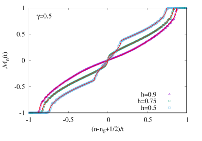
Figure 1: Normalized magnetization profiles (symbols) at $t=200$ compared to the hydrodynamic solution (red solid lines) in (10). The phase transition is located at $h_{c}=1-\gamma^{2}=0.75$.

The Hamiltonian of the XY chain is given by

$$H=-\sum_{n=1}^{N-1}\left(\frac{1+\gamma}{4}\sigma_{n}^{x}\sigma_{n+1}^{x}+\frac{1-\gamma}{4}\sigma_{n}^{y}\sigma_{n+1}^{y}\right)-\frac{h}{2}\sum_{n=1}^{N}\sigma_{n}^{z}$$ (1)

where $\sigma^{\alpha}_{n}$ are Pauli matrices on site $n$, $\gamma$ is the anisotropy and $h$ is a transverse magnetic field. The XY model can be mapped to a chain of free fermions via a Jordan-Wigner (JW) transformation, by introducing the Majorana operators

$$a_{2j-1}=\prod_{k=1}^{j-1}\sigma^{z}_{k}\sigma^{x}_{j},\qquad a_{2j}=\prod_{k=1}^{j-1}\sigma^{z}_{k}\sigma^{y}_{j},$$ (2)

satisfying anticommutation relations $\left\{a_{k},a_{l}\right\}=2\delta_{k,l}$. While the open boundaries in Eq. (1) are most suitable for numerical investigations of the dynamics on finite size chains, for the analytical treatment one should impose antiperiodic boundary conditions $\sigma^{x,y}_{N+1}=-\sigma^{x,y}_{1}$ on the spins, such that $H$ can be brought into a diagonal form by a Fourier transform and a Bogoliubov rotation sm .

We focus on the parameter regime $0<\gamma\leq 1$ and $0\leq h<1$, where the model is in a gapped ferromagnetic phase, with magnetic order in the $x$ direction. In particular, in the limit $N\to\infty$, the ground state is twofold degenerate, with $|0\rangle_{\mathrm{NS}}$ and $|0\rangle_{\mathrm{R}}$ located in the Neveu-Schwarz (NS) and Ramond (R) sectors, corresponding to $\pm 1$ eigenvalues of the parity operator $P=\prod_{k=1}^{N}\sigma^{z}_{k}$, which commutes with the Hamiltonian $\left[H,P\right]$=0. Since both of the ground states are parity eigenstates, their magnetization is vanishing. However, starting from the symmetry-broken ground state $|\Uparrow\,\rangle$, a domain wall initial state can be prepared via a JW excitation, i.e. acting with a single Majorana operator as

$$|\mathrm{JW}\rangle=a_{2n_{0}-1}|\Uparrow\,\rangle,\qquad|\Uparrow\,\rangle=\frac{|0\rangle_{\mathrm{NS}}+|0\rangle_{\mathrm{R}}}{\sqrt{2}}.$$ (3)

In numerical calculations we always consider domain walls localized in the middle of the chain, $n_{0}=N/2+1$.

Our primary goal is to calculate the magnetization profile in the time evolved state

$$\mathrm{e}^{-iHt}|\mathrm{JW}\rangle=\frac{|\phi_{t}\rangle_{\mathrm{NS}}+|\phi_{t}\rangle_{\mathrm{R}}}{\sqrt{2}}$$ (4)

being a superposition of states from the two parity sectors. Both can be obtained by rewriting the excitation in (3) in the fermionic eigenbasis of the Hamiltonian, leading to a superposition of single-particle states. These can then be trivially time evolved and yield sm

$$|\phi_{t}\rangle_{\mathrm{NS}}=\frac{1}{\sqrt{N}}\sum_{q\in\mathrm{NS}}\mathrm{e}^{-i\epsilon_{q}t}\mathrm{e}^{-iq(n_{0}-1)}\mathrm{e}^{i\theta_{q}/2}|q\rangle_{\mathrm{NS}},$$ (5)

where the single-particle dispersion $\epsilon_{q}$ and the Bogoliubov phase $\theta_{q}$ are given by

$$\begin{split}&\epsilon_{q}=\sqrt{(\cos q-h)^{2}+\gamma^{2}\sin^{2}q}\,,\\ &\mathrm{e}^{i(\theta_{q}+q)}=\frac{\cos q-h+i\gamma\sin q}{\epsilon_{q}}\,.\end{split}$$ (6)

The result for $|\phi_{t}\rangle_{\mathrm{R}}$ is completely analogous to (5), with the sum running over momenta $p\in R$. In turn, the normalized magnetization can be cast in the form

$$\mathcal{M}_{n}(t)=\frac{\langle\mathrm{JW}|\sigma^{x}_{n}(t)|\mathrm{JW}\rangle}{\langle\,\Uparrow|\sigma^{x}_{n}|\Uparrow\,\rangle}=\mathrm{Re\,}{{}_{\mathrm{R}}}\langle\phi_{t}|\hat{\mathcal{M}}_{n}|\phi_{t}\rangle_{\mathrm{NS}}\,,$$ (7)

where, in the limit $N\gg 1$, the form factors read Iorgov (2011); Iorgov and Lisovyy (2011)

$${{}_{\mathrm{R}}}\langle p|\hat{\mathcal{M}}_{n}|q\rangle_{\mathrm{NS}}=-\frac{i}{N}\frac{\epsilon_{p}+\epsilon_{q}}{2\sqrt{\epsilon_{p}\epsilon_{q}}}\frac{\mathrm{e}^{i(n-1/2)(q-p)}}{\sin\frac{q-p}{2}}.$$ (8)

Combining the results (5)-(8) and considering the thermodynamic limit, one ends up with a double integral formula for the magnetization sm . Interestingly, this is exactly the same expression as the one found earlier for the transverse Ising (TI) chain Eisler et al. (2016), except that the form of the dispersion and the Bogoliubov angle (6) are now more general. In fact, it is the very presence of the XY anisotropy that will give rise to a peculiar dynamical behavior. The hydrodynamical phase transition is encoded in the $q\ll 1$ expansion of the dispersion

$$\epsilon_{q}\approx\Delta+\frac{h-h_{c}}{2\Delta}q^{2}+c\,q^{4},$$ (9)

where $\Delta=1-h$ is the excitation gap and $h_{c}=1-\gamma^{2}$ is a critical field. The coefficient $c$ has a lengthy expression in terms of $h$ and $\gamma$, satisfying $c>0$ for any $h<h_{c}$. In contrast, the mass term in Eq. (9) becomes negative below the critical field.

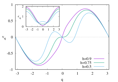
Figure 2: Single-particle velocities $v_{q}$ and dispersion $\epsilon_{q}$ (inset).

While a negative effective mass has no effect on the ground-state properties, it will play a crucial role in the dynamics. Indeed, in a well-defined limit, the shape of the melting domain wall is entirely determined by the group velocities $v_{q}=\frac{\mathrm{d}\epsilon_{q}}{\mathrm{d}q}$. These are shown on Fig. 2 for $\gamma=0.5$, and three different magnetic fields above, below and at the critical value $h_{c}$. In case $h<h_{c}$, the negative slope of $v_{q}$ around $q\to 0$ leads to the development of a new local maximum, which eventually gives rise to a nonanalytic behavior in the hydrodynamic profiles of various observables. In particular, introducing the scaling variable $\nu=(n-n_{0}+1/2)/t$, the magnetization profile reads

$$\mathcal{M}_{n}(t)=1-2\int_{-\pi}^{\pi}\frac{\mathrm{d}q}{2\pi}\Theta(v_{q}-\nu),$$ (10)

where $\Theta(x)$ is the Heaviside step function. The result (10) follows rigorously from a stationary-phase analysis sm of the integral representation of $\mathcal{M}_{n}(t)$, and has a clear physical interpretation. Namely, each single-particle excitation carries a spin-flip Sachdev and Young (1997); Antal et al. (2008); Rieger and Iglói (2011); Kormos et al. (2018) and thus the magnetization along a fixed ray follows from the integrated density of excitations whose speed exceeds $\nu$. Hence, for $h<h_{c}$ the nonanalytical behavior of the density is a consequence of the new branch of solutions around the local maximum for negative momenta.

The comparison between the profiles and the hydrodynamic scaling function is shown on Fig. 1. The magnetization at $t=200$ and various $h$ were calculated for an open chain of size $N=400$ using the Pfaffian formalism described in Eisler et al. (2016). One has an excellent agreement with clear signatures of the developing kink for $h<h_{c}$. The hydrodynamic profile in general depends on the details of the dispersion and is hard to obtain analytically, since the solution of $v_{q}=\nu$ leads to a fourth-order equation. Nevertheless, one expects a universal behavior to emerge around the edge of the front Eisler and Rácz (2013). Indeed, the stationary phase calculation around $v_{q_{*}}=v_{max}$ can be extended to capture the fine structure of the front Viti et al. (2016); Allegra et al. (2016); Perfetto and Gambassi (2017); Kormos (2017), suggesting the following choice for the scaling variable

$$X=(n-n_{0}+1/2+\theta^{\prime}_{q_{*}}/2-v_{q_{*}}t)\left(\frac{2}{|v^{\prime\prime}_{q_{*}}|t}\right)^{1/3}.$$ (11)

In turn, the edge magnetization is given by sm

$$\mathcal{M}_{n}(t)=1-2\left(\frac{2}{|v^{\prime\prime}_{q_{*}}|t}\right)^{1/3}\rho(X)\,,$$ (12)

where $\rho(X)=\left[\mathrm{Ai}^{\prime}(X)\right]^{2}-X\mathrm{Ai}^{2}(X)$ is just the diagonal part of the Airy kernel Tracy and Widom (1994).

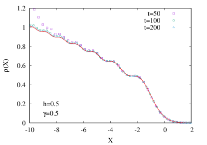
Figure 3: Edge scaling of the magnetization profile, with the scaling variable $X$ and function $\rho(X)$ defined by Eqs. (11) and (12), respectively.

The edge scaling (12) is tested against numerical calculations for $h=\gamma=0.5$ in Fig. 3, showing an excellent agreement already for moderately large times. Note that the larger deviation towards the bulk for $t=50$ is due to the presence of the kink in the profile. In fact, one could ask whether zooming on around the kink would yield a similar universal fine structure as for the edge. However, in the latter case the density has a nonuniversal bulk contribution superimposed, which spoils the step structure. It is also worth noting that the edge scaling (12) for the XY chain can not be derived from a simple higher-order extension of the hydrodynamical picture Fagotti (2017).

The signatures of the hydrodynamical phase transition are also visible on the entanglement profiles, as measured by the von Neumann entropy between the segment $A=\left[1,N/2+r\right]$ and $B$ the rest of the system. Although the XY chain maps to free fermions, extracting the entropy via covariance-matrix techniques for Gaussian states Vidal et al. (2003); Peschel and Eisler (2009) requires some additional care. Indeed, the initial state is excited from the symmetry-broken ground state of the model, which is inherently non-Gaussian Fagotti and Essler (2013). This difficulty can, however, be overcome by the following considerations. Let us denote by $\rho_{\Uparrow}$ the reduced density matrix (RDM) arising from the time evolved state (4) after tracing out the degrees of freedom in $B$. The arrow indicates the choice of the symmetry-broken ground state in (3) and the entropy of the RDM is given by $S(\rho_{\Uparrow})=-\mathrm{Tr\,}\rho_{\Uparrow}\ln\rho_{\Uparrow}$. In fact, one could equally well have defined $\rho_{\Downarrow}$ starting from the spin-reversed initial state, with the entropies of the two RDMs satisfying $S(\rho_{\Uparrow})=S(\rho_{\Downarrow})$ due to obvious symmetry reasons. The main trick is now to consider the convex combination

$$\rho_{G}=\frac{\rho_{\Uparrow}+\rho_{\Downarrow}}{2},$$ (13)

which removes all the parity-odd contributions from the RDMs, albeit still mixing parity-even terms from the two sectors $\mathrm{NS}$ and $\mathrm{R}$. However, in the thermodynamic limit all the expectation values of local operators become equal in both sectors Fagotti and Essler (2013), hence $\rho_{G}$ is equivalent to a Gaussian RDM where the excitation is created upon the parity-symmetric ground state $|0\rangle_{\mathrm{NS}}$.

Due to its Gaussianity, the entropy of $\rho_{G}$ can now be obtained by applying the covariance-matrix formalism as shown in Ref. Caputa and Rams (2017). Indeed, the effect of the Majorana excitation can be represented in a Heisenberg picture

$$a^{\prime}_{k}=a_{2n_{0}-1}a_{k}a_{2n_{0}-1}=\sum_{l=1}^{2N}Q_{k,l}a_{l},\qquad$$ (14)

as an orthogonal transformation on the Majoranas, with matrix elements $Q_{k,l}=\delta_{k,l}(2\delta_{k,2n_{0}-1}-1)$. Similarly, time evolving the state corresponds to the transformation

$$a^{\prime}_{k}(t)=\mathrm{e}^{iHt}a^{\prime}_{k}\mathrm{e}^{-iHt}=\sum_{l=1}^{2N}R_{k,l}a^{\prime}_{l},\qquad$$ (15)

with matrix elements $R_{k,l}$ given as in Ref. Eisler et al. (2016). Hence $\rho_{G}$ corresponds to a RDM associated to the Gaussian state with covariance matrix

$$\tilde{\Gamma}=R\,Q\,\Gamma\,Q^{T}R^{T},$$ (16)

where $i\Gamma_{k,l}={{}_{\mathrm{NS}}}\langle 0|a_{k}a_{l}|0\rangle_{\mathrm{NS}}-\delta_{k,l}$. Note that the matrix $\tilde{\Gamma}$ is exactly the one that appears in the Pfaffian by the calculation of the magnetization Eisler et al. (2016).

Although the entropy of $\rho_{G}$ follows simply via the eigenvalues of the reduced covariance matrix $\tilde{\Gamma}_{A}$ Vidal et al. (2003); Peschel and Eisler (2009), one still has to relate it to the entropy of the non-Gaussian RDM $\rho_{\Uparrow}$ that we are interested in. To this end, one can make use of the inequality for convex combinations of density matrices Lanford and Robinson (1968); Wehrl (1978)

$$S(\sum_{i}\lambda_{i}\rho_{i})\leq\sum_{i}\lambda_{i}S(\rho_{i})-\sum_{i}\lambda_{i}\ln\lambda_{i}\,.$$ (17)

Furthermore, it is also known that the inequality is saturated if the ranges of $\rho_{i}$ are pairwise orthogonal. Applying it to Eq. (13), the orthogonality condition is clearly satisfied due to $\langle\Uparrow|\Downarrow\rangle=0$ and hence one arrives at

$$S(\rho_{\Uparrow})=S(\rho_{G})-\ln 2\,.$$ (18)

The entropy can thus be exactly evaluated using Gaussian techniques.

The result for the profile $\Delta S$, measured from the $t=0$ value, is shown on Fig. 4 at time $t=200$, against the rescaled cut position. The parameters are chosen to be identical to Fig. 1, and a kink for $h=0.5$ emerges again at the value of $r/t$ equal to the local maximum of the velocity $v_{q}$. Furthermore, the entropy growth for the half-chain ($r/t=0$) clearly converges towards the value $\ln 2$, which can be interpreted as a restoration of the spin-flip symmetry in the NESS. Note also the light dip in the middle for $h=h_{c}=0.75$, which is the consequence of a much slower convergence towards the NESS at criticality. The entropy profiles obtained by the Gaussian technique have also been compared to the results of density-matrix renormalization group Schollwöck (2011) calculations, finding an excellent agreement and thus justifying the result in Eq. (18).

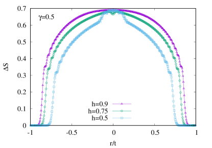
Figure 4: Entanglement profiles as a function of the rescaled distance $r$ of the cut from the middle of the chain. The entropy difference $\Delta S$ from the initial state value is shown at $t=200$ for the same parameter values as in Fig. 1.

We finally consider the normalized equal-time spin-correlation functions $\mathcal{C}_{m,n}(t)={{}_{\mathrm{NS}}}\langle\phi_{t}|\hat{\mathcal{M}}_{m}\hat{\mathcal{M}}_{n}|\phi_{t}\rangle_{\mathrm{NS}}$ which can be studied via the form-factor approach by inserting a resolution of the identity between the operators. Although in general all the multi-particle form factors are nonvanishing, the dominant contribution to the correlations comes from the single-particle terms

$$\mathcal{C}_{m,n}(t)\simeq\sum_{p}{{}_{\mathrm{NS}}}\langle\phi_{t}|\hat{\mathcal{M}}_{m}|p\rangle_{\mathrm{R}}\,{{}_{\mathrm{R}}}\langle p|\hat{\mathcal{M}}_{n}|\phi_{t}\rangle_{\mathrm{NS}}\,.$$ (19)

The above expression can again be evaluated in the hydrodynamic scaling limit and for $m<n$ yields sm

$$\mathcal{C}_{m,n}(t)\simeq 1-2\int_{-\pi}^{\pi}\frac{\mathrm{d}q}{2\pi}\Theta(v_{q}-\mu)\Theta(\nu-v_{q})\,,$$ (20)

where $\mu$ is defined analogously to $\nu$. The integral in (20) gives the number of excitations with velocities between the rays defined by $\mu$ and $\nu$, and has again a simple interpretation. In fact, it is directly related to the difference of the magnetizations along those rays and thus shows similar nonanalytical behavior for $h<h_{c}$.

In the NESS limit $t\to\infty$ with $m,n$ fixed, Eq. (20) predicts long-range magnetic order $\mathcal{C}_{m,n}(t)\to 1$. Together with $\mathcal{M}_{n}(t)\to 0$, this behavior is characteristic of the ground state $|0\rangle_{\mathrm{NS}}$ at large separations $n-m\gg 1$. Furthermore, a careful numerical analysis shows that $\mathcal{C}_{m,n}(t)$ converges towards the proper ground-state value even for small separations of the spins. Indeed, in the ferromagnetic regime the normalized correlators deviate from unity by a term decaying exponentially with the distance Franchini (2017). The source of the discrepancy is the approximation in (19), which neglects the contribution of the multi-particle form factors. A detailed analysis of the correlations will be presented elsewhere Eisler and Maislinger .

In conclusion, our studies of domain-wall melting in the XY chain have revealed a phase transition, manifest in the emergence of kinks in the profiles of various observables. While the critical point $h_{c}=1-\gamma^{2}$ coincides with the one found earlier for open-system dynamics Prosen and Pižorn (2008), the transition exists only in the hydrodynamic regime, and does not survive the NESS limit. In contrast, the latter one seems to be given by the parity-symmetric ground state, which does not show any criticality around $h_{c}$.

Although demonstrated on a simple free-fermion example, there is good reason to believe that this phenomenon carries over to generic integrable systems, where the proper hydrodynamic description has only recently been identified Bertini et al. (2016); Castro-Alvaredo et al. (2016) and applied to initial states with domain walls Piroli et al. (2017); Collura et al. (2018). In particular, the emergence of kinks in the magnetization profile has been observed for the XXZ chain at large anisotropies, resulting from the velocity maxima of the various quasiparticle families that govern the hydrodynamics Piroli et al. (2017). While the mechanism seems to be closely related to the one presented here, it is unclear whether a hydrodynamical phase transition point exists in the XXZ case, since all the profiles considered in Piroli et al. (2017) belong to the kink phase.

Finally, it remains to be understood whether the finite increase of entropy after the JW excitation could be interpreted within a framework similar to the one introduced for local operator insertions in conformal field theories Nozaki et al. (2014). While the results have been checked against the lattice equivalent of local primary excitations for the transverse Ising chain in Ref. Caputa and Rams (2017), it would be interesting to see whether the field theory treatment could be generalized to include the massive case and the non-local operators considered here.

We thank H. G. Evertz and M. Fagotti for discussions. The authors acknowledge funding from the Austrian Science Fund (FWF) through Project No. P30616-N36, and through SFB ViCoM F41 (Project P04).

Supplemental Material:
Hydrodynamical phase transition for domain-wall melting in the XY chain

I Fermionization of XY Hamiltonian

In order to obtain the many-body eigenstates of the XY chain, it is useful to consider periodic $H_{+}$ or antiperiodic $H_{-}$ chains, instead of the open one in Eq. (1). These are given by

$$H_{s}=-\frac{1}{2}\sum_{n=1}^{N}\left(\frac{1+\gamma}{2}\sigma_{n}^{x}\sigma_{n+1}^{x}+\frac{1-\gamma}{2}\sigma_{n}^{y}\sigma_{n+1}^{y}+h\sigma_{n}^{z}\right),$$ (S1)

where the boundary conditions are $\sigma^{x}_{N+1}=s\sigma^{x}_{1}$ and $\sigma^{y}_{N+1}=s\sigma^{y}_{1}$ for $s=\pm$. Since $H_{s}$ commutes with the parity $P$, it can be written in a block-diagonal form

$$H_{s}=\frac{1-sP}{2}H_{\mathrm{R}}+\frac{1+sP}{2}H_{\mathrm{NS}},\qquad P=\prod_{n=1}^{N}\sigma^{z}_{n}\,.$$ (S2)

The parity subspaces are the Ramond (R) and Neveu-Schwarz (NS) sectors, defining two different Hamiltonians. In terms of Majorana operators, obtained via the Jordan-Wigner transformation (2), both of them can be brought into the quadratic form

$$H_{\mathrm{R/NS}}=\frac{i}{2}\sum_{j=1}^{N}\left(\frac{1+\gamma}{2}a_{2j}a_{2j+1}-\frac{1-\gamma}{2}a_{2j-1}a_{2j+2}+ha_{2j-1}a_{2j}\right),\qquad$$ (S3)

where the two Hamiltonians differ only in the boundary conditions $a_{2N+1}=\pm a_{1}$ and $a_{2N+2}=\pm a_{2}$ being periodic for R and antiperiodic for the NS sector. Each sector can be simultaneously diagonalized by a joint Fourier and Bogoliubov transformation

$$a_{2j-1}=\frac{1}{\sqrt{N}}\sum_{q\in\mathrm{R/NS}}\mathrm{e}^{-iq(j-1)}\mathrm{e}^{i\theta_{q}/2}(b_{q}^{\dagger}+b_{-q}),\qquad a_{2j}=\frac{-i}{\sqrt{N}}\sum_{q\in\mathrm{R/NS}}\mathrm{e}^{-iqj}\mathrm{e}^{-i\theta_{q}/2}(b_{q}^{\dagger}-b_{-q}),$$ (S4)

where the allowed values of the momenta are $q_{k}=\frac{2\pi}{N}k$ for R and $q_{k}=\frac{2\pi}{N}(k+1/2)$ for NS, respectively, with $k=-N/2,\dots,N/2-1$. Note that the site index $j$ in the Fourier transformation is shifted by one for odd Majorana operators. This is a dual representation in terms of which the Bogoliubov angle must satisfy

$$\mathrm{e}^{i(\theta_{q}+q)}=\frac{\cos q-h+i\gamma\sin q}{\epsilon_{q}},\qquad\epsilon_{q}=\sqrt{(\cos q-h)^{2}+\gamma^{2}\sin^{2}q}\,.$$ (S5)

In fact, the above definition ensures that $\theta_{q}$ is a continuous and smooth function in its full domain $q\in\left[-\pi,\pi\right]$, for arbitrary parameters $0<\gamma\leq 1$ and $0\leq h<1$ in the ferromagnetic phase. The diagonal form of the Hamiltonian and its many-particle eigenstates then read

$$H_{\mathrm{R/NS}}=\sum_{q\in\mathrm{R/NS}}{\epsilon_{q}}b^{\dagger}_{q}b_{q}+\mathrm{const},\qquad|q_{1},q_{2},\dots,q_{m}\rangle_{\mathrm{R/NS}}=\prod_{i=1}^{m}b^{\dagger}_{q_{i}}|0\rangle_{\mathrm{R/NS}}\,.$$ (S6)

Finally, it should be pointed out that the boundary condition on the spins selects the parity of the many-particle basis: $m=2\ell$ is even for the spin-periodic Hamiltonian $H_{+}$, and $m=2\ell+1$ is odd for the spin-antiperiodic one $H_{-}$.

II Form factor approach

To calculate the time evolution of the magnetization, one also needs the corresponding form factors of the $\sigma^{x}$ operator. In fact, it is more convenient to consider the matrix elements normalized by the equilibrium magnetization, which in the large $N$ limit reads Iorgov (2011); Iorgov and Lisovyy (2011)

$${{}_{\mathrm{R}}}\langle p|\hat{\mathcal{M}}_{n}|q\rangle_{\mathrm{NS}}=\frac{{{}_{\mathrm{R}}}\langle p|\sigma^{x}_{n}|q\rangle_{\mathrm{NS}}}{{{}_{\mathrm{R}}}\langle 0|\sigma^{x}_{n}|0\rangle_{\mathrm{NS}}}=-\frac{i}{N}\frac{\cosh\frac{\Delta_{p}-\Delta_{q}}{2}\sinh\frac{\Delta_{p}+\Delta_{q}}{2}}{\sqrt{\sinh\Delta_{p}\sinh\Delta_{q}}}\frac{\mathrm{e}^{i(n-1/2)(q-p)}}{\sin\frac{q-p}{2}}.$$ (S7)

The above definition of the form factors is well-suited for the parameter regime $\sqrt{1-\gamma^{2}}<h<1$, i.e. in the non-oscillatory ferromagnetic phase Franchini (2017), where the auxiliary parameter $\Delta_{q}$ is defined via

$$\sinh\Delta_{q}=\frac{\sqrt{1-\gamma^{2}}}{\gamma\sqrt{\gamma^{2}+h^{2}-1}}\epsilon_{q}.$$ (S8)

In the oscillatory phase $0<h<\sqrt{1-\gamma^{2}}$ the form factors can be obtained by analytic continuation Iorgov (2011), i.e. by introducing the variable $\tilde{\Delta}_{q}=\Delta_{q}+i\pi/2$. In fact, the form-factor formula (S7) can even be further simplified by making use of the identity

$$\cosh\frac{\Delta_{p}-\Delta_{q}}{2}\sinh\frac{\Delta_{p}+\Delta_{q}}{2}=\frac{1}{2}(\sinh\Delta_{p}+\sinh\Delta_{q}).$$ (S9)

Substituting (S8) and (S9) into (S7), one obtains immediately Eq. (8). Using these form factors and taking the thermodynamic limit, Eq. (7) for the magnetization can be written out as a double integral

$$\mathcal{M}_{n}(t)=\mathrm{Im\,}\int_{-\pi}^{\pi}\frac{\mathrm{d}p}{2\pi}\int_{-\pi}^{\pi}\frac{\mathrm{d}q}{2\pi}\frac{\epsilon_{p}+\epsilon_{q}}{2\sqrt{\epsilon_{p}\epsilon_{q}}}\frac{\mathrm{e}^{i(n-n_{0}+1/2)(q-p)}}{\sin\frac{q-p}{2}}\mathrm{e}^{i(\theta_{q}-\theta_{p})/2}\mathrm{e}^{i(\epsilon_{p}-\epsilon_{q})t}\,.$$ (S10)

Using the properties $\epsilon_{-q}=\epsilon_{q}$ and $\theta_{-q}=-\theta_{q}$, the above expression can be written as $\mathcal{M}_{n}(t)=\mathcal{M}^{e}_{n}(t)+\mathcal{M}^{o}_{n}(t)$ with only two nonvanishing contributions

$$\begin{split}\mathcal{M}^{e}_{n}(t)=\int_{-\pi}^{\pi}\frac{\mathrm{d}p}{2\pi}\int_{-\pi}^{\pi}\frac{\mathrm{d}q}{2\pi}\frac{\epsilon_{p}+\epsilon_{q}}{2\sqrt{\epsilon_{p}\epsilon_{q}}}\frac{\cos\left[(n-n_{0}+1/2)(q-p)\right]}{\sin\frac{q-p}{2}}\sin\frac{\theta_{q}-\theta_{p}}{2}\cos(\epsilon_{p}-\epsilon_{q})t\,,\\ \mathcal{M}^{o}_{n}(t)=\int_{-\pi}^{\pi}\frac{\mathrm{d}p}{2\pi}\int_{-\pi}^{\pi}\frac{\mathrm{d}q}{2\pi}\frac{\epsilon_{p}+\epsilon_{q}}{2\sqrt{\epsilon_{p}\epsilon_{q}}}\frac{\sin\left[(n-n_{0}+1/2)(q-p)\right]}{\sin\frac{q-p}{2}}\cos\frac{\theta_{q}-\theta_{p}}{2}\cos(\epsilon_{p}-\epsilon_{q})t\,.\end{split}$$ (S11)

Hence the magnetization is the sum of an even and an odd function $\mathcal{M}^{e,o}_{n}(t)=\pm\mathcal{M}^{e,o}_{2n_{0}-1-n}(t)$ under reflections with respect to the initial domain wall position. Note that, in general, the even term has a contribution of much smaller magnitude, and it vanishes completely in the hydrodynamic scaling limit. Moreover, in the limit $\gamma=1$ of a transverse Ising chain, the even part $\mathcal{M}^{e}_{n}(t)=0$ vanishes identically even for finite times.

The normalized correlation functions $\mathcal{C}_{m,n}(t)={{}_{\mathrm{NS}}}\langle\phi_{t}|\hat{\mathcal{M}}_{m}\hat{\mathcal{M}}_{n}|\phi_{t}\rangle_{\mathrm{NS}}$ can also be studied through the form factor approach. The standard trick is to insert an identity between the two operators, written in terms of the eigenbasis

$$\openone=\sum_{p}|p\rangle\langle p|+\sum_{p_{1},p_{2}}|p_{1},p_{2}\rangle\langle p_{1},p_{2}|+\sum_{p_{1},p_{2},p_{3}}|p_{1},p_{2},p_{3}\rangle\langle p_{1},p_{2},p_{3}|+\dots$$ (S12)

Thus, in contrast to the magnetization which could be exactly evaluated using only single-particle form factors, the situation for the correlations is much more complicated as an infinite series of many-particle matrix elements appear. Nevertheless, it is reasonable to expect that the dominant contribution to the correlations still comes from the single-particle sector. Hence, we will consider this approximate expression, given by (19) in the main text, which for $N\to\infty$ can be converted into the integral form

$$\mathcal{C}_{m,n}(t)\simeq\int\frac{\mathrm{d}q_{1}}{2\pi}\int\frac{\mathrm{d}q_{2}}{2\pi}\mathrm{e}^{-i(\theta_{q_{1}}-\theta_{q_{2}})/2}\mathrm{e}^{i(\epsilon_{q_{1}}-\epsilon_{q_{2}})t}\int\frac{\mathrm{d}p}{2\pi}\frac{\epsilon_{p}+\epsilon_{q_{1}}}{2\sqrt{\epsilon_{p}\epsilon_{q_{1}}}}\frac{\epsilon_{p}+\epsilon_{q_{2}}}{2\sqrt{\epsilon_{p}\epsilon_{q_{2}}}}\frac{\mathrm{e}^{-i(m-n_{0}+1/2)(q_{1}-p)}}{\sin\frac{q_{1}-p}{2}}\frac{\mathrm{e}^{i(n-n_{0}+1/2)(q_{2}-p)}}{\sin\frac{q_{2}-p}{2}}\,.$$ (S13)

III Stationary phase calculations

The profiles in the hydrodynamic scaling limit can be obtained by stationary phase arguments, and their derivation closely follows the lines of Refs. Viti et al. (2016); Allegra et al. (2016); Perfetto and Gambassi (2017); Kormos (2017). Let us consider first the magnetization as given by Eq. (S10). In the limit $n-n_{0}\gg 1$ and $t\gg 1$, the integrand is highly oscillatory and thus the main contribution comes from around the points $q_{s}$ where the stationarity condition is satisfied

$$v_{q_{s}}t=n-n_{0}+1/2+\theta^{\prime}_{q_{s}}/2,\qquad v_{q}=\frac{\mathrm{d}\epsilon_{q}}{\mathrm{d}q}.$$ (S14)

The stationary phase condition for the integral over $p$ is exactly the same. Moreover, the integrand has a pole at $p=q$ which suggests the change of variables $Q=q-p$ and $P=(q+p)/2$. In the new variables, the stationarity condition is $Q_{s}=0$ for arbitrary values of $P$. One shall thus expand the integrand in (S10) around $Q=0$, setting

$$\frac{\epsilon_{p}+\epsilon_{q}}{2\sqrt{\epsilon_{p}\epsilon_{q}}}\approx 1,\qquad\sin\frac{q-p}{2}\approx\frac{Q}{2},$$ (S15)

to arrive at

$$2\,\mathrm{Re\,}\int_{-\pi}^{\pi}\frac{\mathrm{d}P}{2\pi}\int_{-\infty}^{\infty}\frac{\mathrm{d}Q}{2\pi i}\frac{\mathrm{e}^{i(n-n_{0}+1/2+\theta^{\prime}_{P}-v_{P}t)Q}}{Q}.$$ (S16)

To carry out the integration around the pole, we use a formal identity in complex analysis as well as the integral representation of the Heaviside theta function

$$\frac{1}{Q}=i\pi\delta(Q)+\lim_{\delta\to 0}\frac{1}{Q+i\delta},\qquad\Theta(x)=-\lim_{\delta\to 0}\int_{-\infty}^{\infty}\frac{\mathrm{d}Q}{2\pi i}\frac{\mathrm{e}^{-iQx}}{Q+i\delta}.$$ (S17)

In the hydrodynamic regime one can neglect the term $\theta^{\prime}_{P}$ and introduce the scaling variable $\nu=(n-n_{0}+1/2)/t$, which brings us to the result (10) in the main text.

In general, the hydrodynamic profile is found by solving the equation $v_{q}=\nu$. Special attention is needed around the maximum $v_{q_{*}}=v_{max}$ of the velocities, where the solutions coalesce at momentum $q_{*}$. To get the fine structure of the front edge, one has to expand the dispersion around $q_{*}$ as

$$\epsilon_{q}\approx\epsilon_{q_{*}}+v_{q_{*}}(q-q_{*})+\frac{\epsilon^{\prime\prime\prime}_{q_{*}}}{6}(q-q_{*})^{3}.$$ (S18)

Furthermore, one can introduce the following rescaled variables

$$X=(n-n_{0}+1/2+\theta^{\prime}_{q_{*}}/2-v_{q_{*}}t)\left(\frac{-2}{\epsilon^{\prime\prime\prime}_{q_{*}}t}\right)^{1/3},\quad Q=\left(\frac{-2}{\epsilon^{\prime\prime\prime}_{q_{*}}t}\right)^{-1/3}(q-q_{*}),\quad P=\left(\frac{-2}{\epsilon^{\prime\prime\prime}_{q_{*}}t}\right)^{-1/3}(p-q_{*}).$$ (S19)

Substituting (S18) and (S19) into (7), one arrives at the following integral

$$\left(\frac{-2}{\epsilon^{\prime\prime\prime}_{q_{*}}t}\right)^{1/3}\mathrm{Im\,}\int\frac{\mathrm{d}P}{2\pi}\int\frac{\mathrm{d}Q}{2\pi}\frac{\mathrm{e}^{iX(Q-P)}\mathrm{e}^{i(Q^{3}-P^{3})/3}}{(Q-P)/2}.$$ (S20)

Using the integral representation of the Airy kernel

$$K(X,Y)=\lim_{\delta\to 0}\int\frac{\mathrm{d}P}{2\pi}\int\frac{\mathrm{d}Q}{2\pi}\frac{\mathrm{e}^{-iXP}\mathrm{e}^{-iP^{3}/3}\mathrm{e}^{iYQ}\mathrm{e}^{iQ^{3}/3}}{i(P-Q-i\delta)}=\frac{\mathrm{Ai}(X)\mathrm{Ai}^{\prime}(Y)-\mathrm{Ai}^{\prime}(X)\mathrm{Ai}(Y)}{X-Y},$$ (S21)

one recovers (12) of the main text, where the diagonal terms of the Airy kernel Tracy and Widom (1994) can be obtained as

$$\rho(X)=\lim_{Y\to X}K(X,Y)=\left[\mathrm{Ai}^{\prime}(X)\right]^{2}-X\mathrm{Ai}^{2}(X).$$ (S22)

The stationary phase calculation for the approximation of the correlation function in (S13) is very similar to that for the magnetization. Indeed, introducing the new set of variables

$$Q_{1}=q_{1}-p,\qquad Q_{2}=q_{2}-p,\qquad P=\frac{q_{1}+p}{2},$$ (S23)

and expanding around $Q_{1}=0$ and $Q_{2}=0$, one obtains

$$\mathcal{C}_{m,n}(t)\simeq 4\int\frac{\mathrm{d}P}{2\pi}\int\frac{\mathrm{d}Q_{1}}{2\pi}\frac{\mathrm{e}^{-i(m-n_{0}+1/2+\theta^{\prime}_{P}-v_{P}t)Q_{1}}}{Q_{1}}\int\frac{\mathrm{d}Q_{2}}{2\pi}\frac{\mathrm{e}^{i(n-n_{0}+1/2+\theta^{\prime}_{P}-v_{P}t)Q_{2}}}{Q_{2}}.$$ (S24)

Applying (S17) in both the $Q_{1}$ and $Q_{2}$ integrals, the result can again be written with the help of step functions. Using the property $\Theta(x-x_{1})\Theta(x-x_{2})=\Theta(x-\max(x_{1},x_{2}))$, and introducing the scaling variable $\mu=(m-n_{0}+1/2)/t$ analogously to $\nu$, one arrives at

$$\mathcal{C}_{m,n}(t)\simeq 1-2\int_{-\pi}^{\pi}\frac{\mathrm{d}P}{2\pi}\Theta(v_{P}-\mu)+2\int_{-\pi}^{\pi}\frac{\mathrm{d}P}{2\pi}\Theta(v_{P}-\nu),$$ (S25)

where we assumed $\mu<\nu$. Finally, the difference of the step functions can also be rewritten as a product as in (20).

References

- Sachdev (2011) S. Sachdev, Quantum Phase Transitions (Cambridge University Press, 2011).
- Polkovnikov et al. (2011) A. Polkovnikov, K. Sengupta, A. Silva, and M. Vengalattore, Rev. Mod. Phys. 83, 863 (2011).
- Calabrese et al. (2016) P. Calabrese, F. H. L. Essler, and G. Mussardo, J. Stat. Mech. 064001 (2016).
- Heyl et al. (2013) M. Heyl, A. Polkovnikov, and S. Kehrein, Phys. Rev. Lett. 110, 135704 (2013).
- Heyl (2018) M. Heyl, Rep. Prog. Phys. 81, 054001 (2018).
- Jurcevic et al. (2017) P. Jurcevic, H. Shen, P. Hauke, C. Maier, T. Brydges, C. Hempel, B. P. Lanyon, M. Heyl, R. Blatt, and C. F. Roos, Phys. Rev. Lett. 119, 080501 (2017).
- Eckstein et al. (2009) M. Eckstein, M. Kollar, and P. Werner, Phys. Rev. Lett. 103, 056403 (2009).
- Schiró and Fabrizio (2010) M. Schiró and M. Fabrizio, Phys. Rev. Lett. 105, 076401 (2010).
- Sciolla and Biroli (2010) B. Sciolla and G. Biroli, Phys. Rev. Lett. 105, 220401 (2010).
- Garrahan and Lesanovsky (2010) J. P. Garrahan and I. Lesanovsky, Phys. Rev. Lett. 104, 160601 (2010).
- Diehl et al. (2010) S. Diehl, A. Tomadin, A. Micheli, R. Fazio, and P. Zoller, Phys. Rev. Lett. 105, 015702 (2010).
- Halimeh and Zauner-Stauber (2017) J. C. Halimeh and V. Zauner-Stauber, Phys. Rev. B 96, 134427 (2017).
- Žunkovič et al. (2018) B. Žunkovič, M. Heyl, M. Knap, and A. Silva, Phys. Rev. Lett. 120, 130601 (2018).
- Prosen and Pižorn (2008) T. Prosen and I. Pižorn, Phys. Rev. Lett. 101, 105701 (2008).
- Prosen and Žunkovič (2010) T. Prosen and B. Žunkovič, New. J. Phys. 12, 025016 (2010).
- (16) See Supplemental Material for details.
- Iorgov (2011) N. Iorgov, J. Phys. A: Math. Theor. 44, 335005 (2011).
- Iorgov and Lisovyy (2011) N. Iorgov and O. Lisovyy, J. Stat. Mech. P04011 (2011).
- Eisler et al. (2016) V. Eisler, F. Maislinger, and H. G. Evertz, SciPost Phys. 1, 014 (2016).
- Sachdev and Young (1997) S. Sachdev and A. P. Young, Phys. Rev. Lett. 78, 2220 (1997).
- Antal et al. (2008) T. Antal, P. L. Krapivsky, and A. Rákos, Phys. Rev. E 78, 061115 (2008).
- Rieger and Iglói (2011) H. Rieger and F. Iglói, Phys. Rev. B 84, 165117 (2011).
- Kormos et al. (2018) M. Kormos, C. P. Moca, and G. Zaránd, Phys. Rev. E 98, 032105 (2018).
- Eisler and Rácz (2013) V. Eisler and Z. Rácz, Phys. Rev. Lett. 110, 060602 (2013).
- Viti et al. (2016) J. Viti, J-M. Stéphan, J. Dubail, and M. Haque, Europhys. Lett. 115, 40011 (2016).
- Allegra et al. (2016) N. Allegra, J. Dubail, J-M. Stéphan, and J. Viti, J. Stat. Mech. 053108 (2016).
- Perfetto and Gambassi (2017) G. Perfetto and A. Gambassi, Phys. Rev. E 96, 012138 (2017).
- Kormos (2017) M. Kormos, SciPost Phys. 3, 020 (2017).
- Tracy and Widom (1994) C. A. Tracy and H. Widom, Commun. Math. Phys. 159, 151 (1994).
- Fagotti (2017) M. Fagotti, Phys. Rev. B 96, 220302(R) (2017).
- Vidal et al. (2003) G. Vidal, J. I. Latorre, E. Rico, and A. Kitaev, Phys. Rev. Lett. 90, 227902 (2003).
- Peschel and Eisler (2009) I. Peschel and V. Eisler, J. Phys. A: Math. Theor. 42, 504003 (2009).
- Fagotti and Essler (2013) M. Fagotti and F. H. L. Essler, Phys. Rev. B 87, 245107 (2013).
- Caputa and Rams (2017) P. Caputa and M. M. Rams, J. Phys. A: Math. Theor. 50, 055002 (2017).
- Lanford and Robinson (1968) O. E. Lanford and D. W. Robinson, J. Math. Phys 9, 1120 (1968).
- Wehrl (1978) A. Wehrl, Rev. Mod. Phys. 50, 221 (1978).
- Schollwöck (2011) U. Schollwöck, Annals of Physics 326, 96 (2011).
- Franchini (2017) F. Franchini, An Introduction to Integrable Techniques for One-Dimensional Quantum Systems, vol. 940 of Lecture Notes in Physics (Springer, 2017).
- (39) V. Eisler and F. Maislinger, to be published.
- Bertini et al. (2016) B. Bertini, M. Collura, J. De Nardis, and M. Fagotti, Phys. Rev. Lett. 117, 207201 (2016).
- Castro-Alvaredo et al. (2016) O. A. Castro-Alvaredo, B. Doyon, and T. Yoshimura, Phys. Rev. X 6, 041065 (2016).
- Piroli et al. (2017) L. Piroli, J. De Nardis, M. Collura, B. Bertini, and M. Fagotti, Phys. Rev. B 96, 115124 (2017).
- Collura et al. (2018) M. Collura, A. De Luca, and J. Viti, Phys. Rev. B 97, 081111(R) (2018).
- Nozaki et al. (2014) M. Nozaki, T. Numasawa, and T. Takayanagi, Phys. Rev. Lett. 112, 111602 (2014).