Compact objects in scalar-tensor theories after GW170817

Abstract

The recent observations of neutron star mergers have changed our perspective on scalar-tensor theories of gravity, favouring models where gravitational waves travel at the speed of light. In this work we consider a scalar-tensor set-up with such a property, belonging to a beyond Horndeski system, and we numerically investigate the physics of locally asymptotically flat black holes and relativistic stars. We first determine regular black hole solutions equipped with horizons: they are characterized by a deficit angle at infinity, and by large contributions of the scalar to the geometry in the near horizon region. We then study configurations of incompressible relativistic stars. We show that their compactness can be much higher than stars with the same energy density in General Relativity, and the scalar field profile imposes stringent constraints on the star properties. These results can suggest new ways to probe the efficiency of screening mechanisms in strong gravity regimes, and can help to build specific observational tests for scalar-tensor gravity models with unit speed for gravitational waves.

I Introduction

Scalar-tensor theories with non-minimal couplings between scalar fields and gravity find interesting applications to cosmology (dark energy and dark matter problems, see e.g. the review Clifton:2011jh ) and quantum gravity (including Lorentz violating systems as Horava-Lisfshitz gravity, see Wang:2017brl for a recent review). Moreover, they are able to screen fifth forces by means of the Vainshtein mechanism (see for example Amendola:1993uh ; Kimura:2011dc ; Babichev:2013usa ; Bellini:2015wfa ). Over the years, many advances have been made in developing consistent scalar-tensor theories, going from Brans-Dicke systems Brans:1961sx , to Galileons and Horndeski theories Nicolis:2008in ; Horndeski:1974wa , to beyond Horndenski and DHOST/EST scenarios Gleyzes:2014dya ; Zumalacarregui:2013pma ; Langlois:2015cwa ; Crisostomi:2016czh ; BenAchour:2016fzp ; Crisostomi:2016tcp . The study of black holes and compact relativistic stars in these richer scalar-tensor theories is relevant for phenomenological investigations of screening mechanisms inside compact sources Herdeiro:2015waa ; Sakstein:2015aac ; Silva:2016smx ; Sakstein:2016oel , and for our theoretical understanding of no-hair and singularity theorems in Einstein General Relativity (GR) non-minimally coupled with scalar fields (see e.g. the discussion in Bekenstein:1996pn ). The purpose of this work is to investigate asymptotically flat black holes and relativistic stars in a class of scalar-tensor theories compatible with the stringent constrains recently obtained from the observation of neutron star mergers.

Asymptotically flat black hole solutions with non-trivial scalar profiles have been found in Horndeski gravity (see Babichev:2016rlq for a review), and some are known for beyond Horndeski theories Babichev:2017guv . A non-vanishing scalar field profile may or may not affect the properties of the geometry. Even if black hole solutions in these theories exhibit only small deviations from their GR counterparts, it is possible that scalar field effects become more relevant in presence of matter, thus leading to sizeable consequences that can be constrained with observational data. This phenomenon was first pointed out in a theory of Brans-Dicke gravity applied to neutron star objects in Damour:1993hw ; Damour:1996ke ; Salgado:1998sg and dubbed spontaneous scalarisation; it has also been analysed recently in more general scalar-tensor theories Chagoya:2014fza ; Kobayashi:2014ida ; Crisostomi:2017lbg ; Dima:2017pwp ; Silva:2017uqg . Investigations of explicit solutions for compact relativistic objects are necessary for acquiring a better understanding of how these systems can be distinguished from GR. Studies along these lines typically focus on neutron stars, since the strong gravitational field around these objects provides a good laboratory to test modified gravity theories. These investigations have shown that configurations compatible – within the error bars – with the measured masses and radii of neutron stars are common in scalar-tensor gravity Cisterna:2015yla ; Maselli:2016gxk ; Babichev:2016jom . The analysis of these systems in modified gravity is at an early stage in comparison with the theoretical advances made in GR over the past decades, although new developments concerning equation-of-state independent relations between properties of relativistic compact objects indicate promising tools to constrain modified gravity theories Pani:2014jra ; Pappas:2014gca ; Gupta:2017vsl .

Recently, gravitational and electromagnetic radiation emitted by NS mergers was detected almost simultaneously by LIGO, VIRGO, and an array of observatories on earth and in space TheLIGOScientific:2017qsa , placing a strong constraint on the difference between the propagation speed of gravitational waves ($c_{GW}$) and the speed of light, $-3\times 10^{-15}\leq c_{GW}-1\leq 7\times 10^{-16}$ Monitor:2017mdv , where the speed of light is normalized to unity. Besides the quadratic and cubic Horndeski Lagrangians, scalar-tensor theories of gravity generically predict gravitational waves that do not travel at the speed of light. There are, on the other hand, particular combinations of Horndeski and beyond Horndeski Lagrangians which predict $c_{GW}=1$ Ezquiaga:2017ekz ; Creminelli:2017sry ; Sakstein:2017xjx ; Baker:2017hug . Observational consequences of these Lagrangians have been recently analysed, and it has been shown that – in absence of a canonical kinetic term for a scalar field – the screening mechanism allows to recover exact GR solutions in vacuum, although screening effects are broken in presence of matter Crisostomi:2017lbg ; Dima:2017pwp .

On the other hand, on general physical grounds we expect that the standard scalar kinetic term should be present in the scalar action, being the leading dimension four operator that governs the scalar dynamics, at least around nearly flat backgrounds. In this paper we focus on a specific scalar-tensor theory that includes, besides the kinetic term of the scalar field, a combination of quartic Horndeski and beyond Horndeski contributions satisfying the condition $c_{GW}=1$. The presence of the standard kinetic terms affects considerably the geometry, and we find several new phenomena associated with the non-linearity of our system of equations. In Section II we present the theory under consideration. In Section III we determine the conditions to satisfy for obtaining (locally) asymptotically flat black hole solutions supporting a non-trivial scalar field profile. We numerically analyse how the scalar affects the size of the horizons, and we find conditions to avoid naked singularities. The corresponding solutions are characterized by a deficit angle induced by the scalar field kinetic terms. In Section IV we proceed to study relativistic compact objects in this theory and we find that, in contrast to other scenarios of beyond Horndeski systems, the angular deficit does not produce a singularity at the centre of these objects. The non-linearities of the equations lead to new phenomenological consequences, as for example specific relations between radius and energy content of the objects we investigate. By matching interior and exterior solutions we find situations where the scalar field contributions to the geometry are dominant inside a compact object, but negligible in the exterior, pointing towards a sizeable breaking of a Vainshtein screening mechanism. Finally, we discuss how the compactness of this scalar-tensor configurations, and the deficit angle itself, can be used to constrain this theory.

II Theories of Horndeski and beyond after GW170817

The most general scalar-tensor theory leading to second order equations of motion is a combination of the Horndenski Lagrangians Horndeski:1974wa . Calling $\phi$ the scalar field, such Lagrangian densities are Deffayet:2011gz ; Kobayashi:2011nu

$$\mathcal{L}_{2} =G_{2},\hskip 30.00005pt$$

$$\mathcal{L}_{3} =G_{3}\,[\Phi]\,,$$

$$\mathcal{L}_{4} =G_{4}R+G_{4,X}\left\{[\Phi]^{2}-[\Phi^{2}]\right\},$$

$$\mathcal{L}_{5} =G_{5}G_{\mu\nu}\Phi^{\mu\nu}-\frac{1}{6}G_{5,X}\left\{[\Phi]^{3}-3[\Phi][\Phi^{2}]+2[\Phi^{3}]\right\},$$ (1)

where $\Phi$ is a matrix with components $\nabla^{\mu}\nabla_{\nu}\phi$ , and

$$X= -\frac{1}{2}\,\partial_{\mu}\phi\partial^{\mu}\phi\,,$$

$$\left[\Phi^{n}\right]= \,{\text{tr}}\left(\Phi^{n}\right)\,,$$

$$\langle\Phi\rangle= \,\partial^{\mu}\phi\partial_{\mu}\partial_{\nu}\phi\partial^{\nu}\phi\,.$$ (2)

$G_{i}$ are arbitrary functions of $\phi$ and $X$, or only of $X$ if we impose a shift symmetry $\phi\to\phi+$const. The equations of motion associated with Lagrangians (1) are second order ensuring that the system is free of Ostrogradsky instabilities. On the the other hand, it is possible to have healthy scalar-tensor theories also with higher order equations of motion, provided that constraint conditions forbid the propagation of would-be Ostrogradsky ghosts. Explicit examples are the theories of beyond Horndeski Gleyzes:2014dya , and their generalizations dubbed DHOST/EST theories Langlois:2015cwa ; Crisostomi:2016czh . The theory of beyond Horndeski is constructed with the Lagrangian densities

$$\mathcal{L}_{4}^{bH} =-\frac{1}{2}F_{4}\,\epsilon^{\mu\nu\rho}{}_{\sigma}\epsilon^{\mu^{\prime}\nu^{\prime}\rho^{\prime}\sigma}\partial_{\mu}\phi\partial_{\mu^{\prime}}\phi\Phi_{\mu\mu^{\prime}}\Phi_{\nu\nu^{\prime}}\Phi_{\rho\rho^{\prime}}\,,$$

$$\mathcal{L}_{5}^{bH} =F_{5}\,\epsilon^{\mu\nu\rho\sigma}\epsilon^{\mu^{\prime}\nu^{\prime}\rho^{\prime}\sigma^{\prime}}\partial_{\mu}\phi\partial_{\mu}^{\prime}\phi\Phi_{\nu\nu^{\prime}}\Phi_{\rho\rho^{\prime}}\Phi_{\sigma\sigma^{\prime}}\,,$$ (3)

with $F_{4,\,5}$ arbitrary functions of $\phi$, $X$. Theories described by a combination of the previous Lagrangians – apart from systems only containing $\mathcal{L}_{2}$ and $\mathcal{L}_{3}$ – generally lead to a modification of the speed of propagation of gravity waves, hence they are disfavoured by the recent observation of gravitational waves from a neutron star merger GW170817 and its associated electromagnetic counterpart GRB 170817A. On the other hand, there are specific combinations of the Horndeski and beyond Horndeski Langrangians which do not change the speed of gravitational waves Bettoni:2016mij . A particular example is the combination

$$\mathcal{L}_{c} =X+\mathcal{L}_{4}+\mathcal{L}_{4}^{bH},\hskip 10.00002pt\text{with }F_{4}=G_{4,X}/X\,,$$

$$=X+G_{4}R+\frac{G_{4,X}}{X}\left(\langle\Phi^{2}\rangle-\langle\Phi\rangle[\Phi]\right)\,,$$ (4)

which we consider in this work. This Lagrangian density includes the standard scalar kinetic term, accompanied by derivative self-interactions and non-minimal couplings with the metric which become important in strong gravity regimes such as in proximity of black holes or in dense objects. For simplicity, and definiteness, we study this theory with the function $G_{4}$ chosen as

$$G_{4}=M_{Pl}^{2}+\frac{\beta}{M_{Pl}^{2}}\,X\,,$$ (5)

where $\beta$ is a dimensionless constant. Black hole configurations for similar systems have been studied in the past both in beyond Horndeski and vector-tensor theories Gripaios:2004ms ; Tasinato:2014eka ; Heisenberg:2014rta . In particular, a stealth Schwarzschild solution was fist discovered for vector-tensor systems with the same choice of $G_{4}$ and a special value of $\beta$ Chagoya:2016aar . When the time component $A_{0}$ of the vector is constant, this solution is equivalent to a scalar-tensor stealth configuration for a scalar field of the form $\phi\,=\,q\,t+\phi_{1}(r)$, with a constant $q$ Babichev:2013cya . Further generalisations based on this solution can be found in Heisenberg:2017hwb ; Chagoya:2017fyl , where neutron stars and asymptotically flat black holes are constructed for arbitrary values of $\beta$ and vector-tensor generalisations of (5).

In this work we focus on the scalar-tensor theory (4), studying new black hole solutions in vacuum with novel features (Section III), and the physics of gravitationally bound compact objects made of incompressible matter (Section IV).

III Black holes

The study of black hole solutions in vacuum for scalar-tensor theories with non-minimal couplings to gravity is interesting at least for two reasons. First, it allows to probe a strong gravity regime for the theory one considers, where non-perturbative contributions to screening mechanisms can make manifest sizeable deviations from GR results (see, e.g. Saito:2015fza ; Koyama:2015oma ). Second, it allows to test no-hair and singularity theorems in new settings, possibly revealing new geometries or topologies characterized by additional scalar charges (see, e.g. Achucarro:1995nu ; Bekenstein:1996pn ). In this section we aim to investigate whether there exist asymptotically flat black hole configurations for the beyond Horndeski theory of Lagrangian (4), answering almost affirmatively – in the sense that we find locally asymptotically flat black hole solutions, for which the curvature invariants vanish for large $r$, but that are characterized by a constant angular deficit at infinity. The existence of an angular deficit in beyond Horndeski theories was first identified in DeFelice:2015sya as a potential source of singularities at the centre of configurations of matter. As we show below, both in vacuum and inside compact objects the angular deficit of the model we are considering does not affect the regularity of the solutions, provided that some conditions are satisfied.

The covariant form of the equations of motion (EOMs) for the the scalar $\phi$ and the metric $g_{\mu\nu}$ is given in Appendix A. Since we are interested on static, spherically symmetric space-times, we start imposing the following Ansatz for the metric

$$ds^{2}=-f(r)dr^{2}+h(r)^{-1}dr^{2}+r^{2}d\theta^{2}+r^{2}\sin^{2}\theta d\varphi^{2}\,,$$ (6)

while we allow for a linear time dependence in the scalar configuration

$$\phi=M_{Pl}^{2}\phi_{0}\,t+\phi_{1}(r)\,,$$ (7)

where $\phi_{0}$ is a dimensionless constant. This Ansatz for the scalar field is compatible with a static spacetime (recall that the equations of motion always contain derivatives of the scalar) and have been extensively studied in the recent literature on scalar-tensor black hole solutions, since the time dependence explicitly breaks the assumptions of no-hair theorems in Horndeski theory Babichev:2016rlq , thus opening up the possibility of finding asymptotically flat black holes dressed with a scalar field (see, e.g. Babichev:2013cya ; Babichev:2016rlq ; Babichev:2017guv , and the review Herdeiro:2015waa ).

Using these Ansatz for metric and scalar, we find that the $(t,r)$ component of the metric EOMs (the $\xi_{tr}$ component in eq (40)) reduces to an algebraic condition for the derivative of the radial scalar field profile $\phi_{1}$, which reads

$$\frac{\beta\phi^{\prime}_{1}\left[f^{2}h(h+1)\phi^{\prime}_{1}{}^{2}+f\left(h^{2}r\phi^{\prime}_{1}{}^{2}f^{\prime}+\phi_{0}^{2}\left(rh^{\prime}-1\right)+h\phi_{0}^{2}\right)-2hr\phi_{0}^{2}f^{\prime}\right]}{fr^{2}\left(fh\phi^{\prime}_{1}{}^{2}-\ \phi_{0}^{2}\right)}+\frac{1}{2}\phi^{\prime}_{1}\,=\,0\,.$$ (8)

If one chooses $\beta\,=0$ – corresponding to GR plus a standard kinetic term for the scalar field – the only solution of the previous equation is $\phi^{\prime}_{1}\,=\,0$. On the other hand, if $\beta\neq 0$, we have a cubic equation for $\phi_{1}^{\prime}$, which additionally admits the following two branches of solutions:

$$\phi_{1}^{\prime}=\pm\phi_{0}\sqrt{\frac{4\beta hrf^{\prime}+fh^{2}r^{2}+2\beta fh^{2}+2\beta frh^{\prime}-2\beta fh}{2\beta f^{2}+f^{2}hr^{2}+2\beta f^{2}h+2\beta frf^{\prime}}}\,.$$ (9)

Notice that such branches are well defined also in the limit $\beta\to 0$, giving $\phi_{1}^{\prime}=\pm\phi_{0}$: hence these branches are disconnected from the $\beta=0$ branch, even when $\phi_{0}$ is turned on. The presence of different branches is common in Horndeski and beyond Horndeski theories where the scalar field derivative satisfies a non-linear algebraic equation, and the non-trivial scalar field profile is responsible for providing a screening mechanism that recovers GR solutions in the strong gravity regime Babichev:2013usa ; Babichev:2016jom ; Crisostomi:2017lbg ; Dima:2017pwp . In what follows, we will concentrate on the upper branch of the algebraic solution (9). The remaining independent equations, that we take as the $(t,t)$ and $(r,r)$ components of the metric equations, are hard to solve exactly for $f,\,h$, but we can study the system numerically, or analytically in certain regimes.

Flat space, corresponding to the choice $f\,=\,h\,=\,1$ using Ansatz (6), is not a solution of the EOMs. Asymptotically de Sitter solutions can be easily found (very similar to the ones originally found in Rinaldi:2012vy ), but here we will focus on black hole solutions that are at least locally asymptotically flat. This branch of solutions has been less studied in the literature, and it is important to investigate in detail the corresponding phenomenology. In order to take into account local instead of global flatness, it is compulsory to slightly generalize the metric Ansatz (6) by including a deficit angle,

$$ds^{2}=-f(r)dt^{2}+h(r)^{-1}dr^{2}+s_{0}^{-1}\,r^{2}d\Omega^{2}\,,$$ (10)

with $s_{0}$ not necessarily equal to one. This modification does not change the branch structure of the solutions of the scalar field equation. With such Ansatz, it is possible to analytically determine asymptotic solutions for the functions $f,\,h$ expanded in inverse powers of the radial distance $r$, imposing the condition that $f\,=\,h\,=\,1$ at asymptotic infinity. The corresponding equations of motion with this Ansatz are given in (41-43). We find, up to second order in an $1/r$ expansion,

$$s_{0} ={1-3\beta\phi_{0}^{2}}\,,$$ (11)

$$f(r) =1-\frac{2M}{r}-\frac{4\beta^{2}\phi_{0}^{2}\left(\beta\phi_{0}^{2}-2\right)}{r^{2}}+{\cal O}\left(\frac{1}{r^{3}}\right)\,,$$ (12)

$$h(r) =1-\frac{2M}{r}+\frac{4\beta^{2}\phi_{0}^{2}\left(1-\beta\phi_{0}^{2}\right)}{r^{2}}+{\cal O}\left(\frac{1}{r^{3}}\right)\,\,,$$ (13)

$$\phi^{\prime}_{1}(r) =\phi_{0}+\frac{2M\phi_{0}}{r}+\frac{2\phi_{0}\left[2\beta^{3}\phi_{0}^{4}+\left(2M^{2}-\beta\right)-3\beta^{2}\phi_{0}^{2}\right]}{r^{2}}+{\cal O}\left(\frac{1}{r^{3}}\right)\,\,,$$ (14)

with $M$ an integration constant. We notice that, since $s_{0}\neq 1$, the geometry has a deficit angle: this is a consequence of including the kinetic terms of the scalar in our action. On the other hand, the radial dependence of the functions $f$, $h$ gives us hope that a would-be conical singularity at the origin $r=0$ can be absent, or covered by horizons. In what follows, we discuss conditions for ensuring that this is the case for the system under consideration. Notice that, besides the deficit angle, the standard ‘$1-2M/r$’ behaviour (plus subleading corrections) of the metric components indicates that the metric is asymptotically flat and approaches GR results at large distances.

Conical deficits covered by horizons have a long history in black hole physics, starting from Aryal:1986sz , and physical realizations and interpretations – related with strings piercing the black hole horizons in Abelian-Higgs models Achucarro:1995nu – can be subtle Bekenstein:1996pn . It is interesting that conical deficits appear also in the context of a single scalar field coupled with gravity, and we will later attempt to connect them with no hair theorems for this system. Geometries with similar deficit angles arise when considering gravitational monopoles Barriola:1989hx ; Shi:2009nz ; Nucamendi:1996ac .

The presence of conical singularities in solutions of beyond Horndeski theories has been first pointed out in DeFelice:2015sya ; Kase:2015gxi : they focus on systems that are not shift symmetric, finding harmful conical singularities at the origin unless the parameters of the theory are appropriately tuned. A set-up more similar to ours has been analysed in a vector-tensor system Heisenberg:2016lux , showing that conical singularities can then be avoided. We will make more detailed comparisons with these works in later Sections.

III.1 Numerical evidence for regular black holes

We now provide numerical evidence that spherically symmetric, locally asymptotically flat solutions of the EOMs (41-43) are free of naked conical singularities at the origin, when appropriate conditions are satisfied. As we shall see, despite the fact that the solution for the metric components has the standard $1/r$ behaviour at large distances from the origin, there arise large deviations from GR configurations near the black hole horizon.

We numerically solve equations (41-43), using the asymptotic fields given in eqs. (12) and (13) as boundary conditions, and proceed integrating inwards towards small $r$ until we encounter the position $r_{h}$ of a horizon, defined by the condition $g^{rr}=h(r_{h})=0$. The system of equations (41-43) is reduced to two equations for $f$ and $h$, since we impose $s_{0}=1-3\beta\phi_{0}^{2}$ and we algebraically solve the equation $\xi_{tr}\,=\,0$ for $\phi_{1}^{\prime}$. We fix $\beta=1$, so that the size of the angular deficit is controlled only by the scalar parameter $\phi_{0}$. The boundary conditions are then specified in terms of two quantities: the black hole mass $M$, and $\phi_{0}$. For definiteness we fix $M=0.5$ (recall that we work in units where $M_{Pl}=1$) and construct black hole solutions characterised by different values of $\phi_{0}$. In order to ensure that the conical deficit is positive ($s_{0}>0$ in eq (10)), we limit our investigation to the interval $0\leq\phi_{0}<1/\sqrt{3\beta}\sim 0.57$. Our numerical results are shown in Fig. 1.

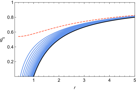
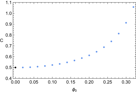
Figure 1: Numerical BH solutions for $2M=\beta=1$. The left panel shows the metric component $g_{rr}$ in GR (black line) and in the theory we consider, with $\phi_{0}$ spanning between $0.02$ and $0.32$ (blue lines). The size of the black hole horizon decreases as $\phi_{0}$ increases. For $\phi_{0}\gtrsim 0.40$ we do not find solutions that form an event horizon. The dashed line shows a solution for $\phi_{0}=0.41$. The compactness of these black holes is shown in the right panel.

The left panel of Fig. 1 shows $h(r)$ – the inverse of the radial metric component. The black line shows the quantity $h(r)$ for the Schwarzschild metric, and the blue lines correspond to different values of $\phi_{0}$ between $0.02$ and $0.32$. For each of the blue lines the function $h(r)$ crosses zero, indicating the position of an horizon, whose size shrinks as $\phi_{0}$ increases. Solutions for $0.32<\phi_{0}\lesssim 0.40$ can be found as well, but they require a higher numerical precision near the horizon. For $\phi_{0}\gtrsim 0.40$ we do not find regular solutions equipped with an horizon: an interpretation for this fact will be provided below.

The right panel shows the compactness of such black holes,

$$C_{BH}=\frac{M}{r_{h}},$$ (15)

where $r_{h}$ is the radius of the event horizon, and $M=0.5$ is fixed by means of the asymptotic conditions (12) and (13). The point in black is the compactness of the Schwarzschild black hole, $C_{Schw}=0.5$. The compactness increases non-linearly with $\phi_{0}$, showing that – thanks to the ${\cal O}(1/r^{2})$ corrections to the metric – our solutions are different from the Schwarzschild configuration when approaching the horizon.

Let us return to specifically discuss the behaviour of the system for $\phi_{0}\gtrsim 0.40$. For our values of $M=0.5$ and $\beta=1$, we could not find solutions with an event horizon for $\phi_{0}\gtrsim 0.40$. Indeed, when changing from $\phi_{0}=0.40$ to $\phi_{0}=0.41$ the solution for the radial metric component changes drastically from profiles like those shown in the blue lines of Fig. 1 to a profile as the one shown in red in the same figure. This limiting value of $\phi_{0}$ is well lower than the bound one would infer from requiring the angular part of the metric to have a positive signature, $\phi_{0}<0.57$. The reason for this behaviour is the following: for any given $\phi_{0}$, there exists a corresponding minimum mass $M_{min}$ that the black hole must have, in order for ensuring that $\phi(r)$ is real everywhere. For $\phi_{0}\gtrsim 0.40$ the minimum mass is larger than $M=0.5$ (the mass value we assumed in our numerical analysis). If the value of the black hole mass is less than $M_{min}$, the scalar field becomes imaginary at a finite radius $r_{c}>0$ (depending on $M_{min}$). In this regime, since the action and equations of motion remain real after the replacement $\phi\to i\phi$, one might accept the possibility that the scalar field can be imaginary, and a solution with real metric can be found for $r<r_{c}$. The metric components $g_{tt}$ and $g^{rr}$ match continuously to the solution for $r>r_{c}$: but they and the Ricci scalar diverge at $r=0$. In order to avoid such singular geometries, associated with imaginary scalar fields, we must require that the mass parameter $M$ characterizing the metric components $f(r)$, $h(r)$ is larger than $M_{min}$. It would be interesting to find a dynamical method to generate such minumum mass for the system.

We can numerically plot the behaviour of the solutions for the set-up we are considering. The left panel of Fig. 2 shows the behaviour of the scalar field solution near the minimum mass $M_{min}$ corresponding to $\phi_{0}=0.30$. For $M>M_{min}$, the spacetime has an event horizon, and $\phi^{\prime}$ diverges there, but the geometry and the trace of the energy-momentum tensor are regular at the horizon. For $M=M_{min}$ the spacetime is regular everywhere and does not have horizons, as shown in the right panel of Fig. 2. This is the only solution for which $\phi^{\prime}_{1}$ is always real and vanishes precisely at $r=0$. For $M<M_{min}$, $\phi^{\prime}_{1}$ vanishes at $r_{c}$. This solution can be extended to $r<r_{c}$ if the scalar field is allowed to be imaginary, at the price of introducing a naked singularity in the geometry.

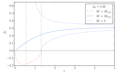
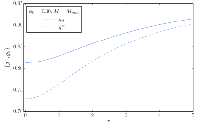
Figure 2: Vacuum geometries. The left panel shows $\phi_{1}^{\prime}$ for a black hole geometry (dashed line) with horizon represented by the dashed vertical line, a regular geometry (solid line), and a singular geometry. The radius $r_{c}$ where the scalar field becomes imaginary in the singular case is indicated by the dotted vertical line, and the region $r<r_{c}$ shows the opposite of the norm of $\phi_{1}^{\prime}$. The right panel shows the metric fields of the regular geometry, which exists only for $M=M_{\min}$.

In summary, for $M>M_{min}$ we have black hole geometries with an event horizon, for $M=M_{min}$ we have a regular geometry without horizons, and for $M<M_{min}$ we have geometries that do not have a horizon, but they become singular in a region where the scalar field is imaginary: in order to have a regular geometry, we need to impose $M\geq M_{min}$. A similar situation exists in quartic Horndeski models with a scalar field that depends only on $r$, where a minimum mass that separates black holes from naked singularities is given in terms of the coupling constants of the model, which also determine the (secondary) asymptotic scalar hair Babichev:2017guv . Another analogy is the Reissner-Nordstrom black hole: given a electric charge $Q$, a minimum black hole mass is required to keep the singularity at $r=0$ protected by an event horizon.

By repeating the analysis described above for different values of $\phi_{0}$, we numerically found that the minimum mass depends quadratically on $\phi_{0}$.

Despite the fact that the geometry does not correspond to flat space at spatial infinity, the curvature invariants go to zero, so the space-time is locally asymptotically flat, and the black hole is isolated and not affected by far away contributions to the energy momentum tensor. The asymptotic properties of the black hole geometry seem to depend on the scalar field properties, through the deficit angle $s_{0}$, which at first sight enters in the computation of asymptotic charges. On the other hand, some care is needed to compute the gravitational mass through an ADM integral in theories with deficit angles. This topic has been clarified in Nucamendi:1996ac for a geometry with the same asympotics as ours. Their work explains that the ADM energy should be properly normalized by the total angular volume of the asymptotic geometry, which includes the deficit angle. Following their procedure, we find that the ADM mass for our system is

$$M_{ADM}\,=\,M\,$$ (16)

with $M$ the coefficient of the $1/r$ terms in the metric components $f$, $h$. Since the gravitational ADM mass is the only asymptotic charge for these black hole configurations, and it does not depend on the scalar parameter $\phi_{0}$, we conclude that our black holes do not have scalar hairs . This conclusion is in agreement with the recent paper Tattersall:2018map .

IV Relativistic compact objects

In this Section we analyse non-singular, gravitationally bound star-like objects with spherical symmetry, studying how the non-minimally coupled scalar field we consider modifies their properties with respect to GR configurations. We find numerical solutions that represent sizeable deviations from GR solutions when the scalar parameter $\phi_{0}$ is large (see our scalar Ansatz (7)), and that are nevertheless connected to GR in the limit $\phi_{0}\to 0$. Using the results of the previous Section, we match the interior configurations for these compact objects to the exterior solutions we previously determined, in order to investigate the efficiency of Vainshtein screening right outside our configurations describing compact objects.

We wish to study static, spherically symmetric configurations of matter minimally coupled to gravity,

$$S=\int d^{4}x\sqrt{-g}\mathcal{L}_{c}+S_{m}\,,$$ (17)

where $\mathcal{L}_{c}$ is defined in eq. (4), and the matter action defines the corresponding matter energy-momentum tensor as

$$T_{\mu\nu}=-\frac{2}{\sqrt{-g}}\frac{\delta S_{m}}{\delta g^{\mu\nu}}.$$ (18)

The equations of motion for the metric result in

$$\xi_{\mu\nu}\,=\,T_{\mu\nu}\,,$$ (19)

where $\xi_{\mu\nu}$ is the tensor defined in eq (40), including metric and scalar contributions. We consider a perfect fluid, so that the only non-vanishing components of the energy-momentum tensor are

$$T^{t}_{t}=-\rho(r),\ \ T^{i}_{j}=p(r)\delta_{j}^{i},$$ (20)

where the Latin indices denote the spatial components of the energy-momentum tensor, and $\rho$ and $p$ characterise the density and pressure of the perfect fluid.

We take the metric Ansatz (10), with

$$s_{0}\equiv 1-3\beta\phi_{0}^{2}\,.$$ (21)

In this way we guarantee that these solutions are in the same coordinate frame as the exterior solutions determined in the previous section. The fluid energy density and pressure can then be expressed in terms of the metric components and scalar field through the relations

$$\rho(r)\,=\,-\xi_{0}^{\,\,0}(r)\,\hskip 14.22636pt,\hskip 14.22636pt\,p(r)\,=\,\xi_{r}^{\,\,r}(r)\,,$$ (22)

with $\xi_{r}^{\,\,r}$ the $(r,r)$ component of the tensor $\xi_{\mu}{}^{\nu}$ obtained by raising one index in equation (40). In order to describe the fluid we also need to consider an equation of state. We will consider configurations of constant density,

$$\rho(r)\,=\,\rho_{0}\,.$$ (23)

Although it is not fully realistic, this set-up allows us to obtain some analytic results, as well as exact numerical solutions. We are interested in configurations that are everywhere regular: we impose that $f^{\prime}(0)\,=\,h^{\prime}(0)\,=\,p^{\prime}(0)\,=\,0$ to ensure regularity at the origin of the configuration. The radial size $R_{s}$ of the compact object is defined as the point where the pressure profile for matter vanishes, $p(R_{s})\,=\,0$.

Since the energy-momentum tensor is diagonal and matter is not directly coupled to the scalar field, the component $\xi_{tr}$ of the metric equations of motion and the scalar field equation remain unchanged with respect to the vacuum case, and can be solved algebraically for $\phi_{1}^{\prime}$. In addition to the Einstein and scalar field equations, we impose the condition that the matter energy-momentum tensor is covariantly conserved,

$$\nabla_{\mu}T^{\mu}{}_{\nu}=0.$$ (24)

For an incompressible star with constant density, the previous condition gives a first order differential equation for $f(r)$ with solution ($f_{0}$ is a constant)

$$f(r)\,=\,f_{0}\left(p(r)+\rho_{0}\right)^{-2}.$$ (25)

Plugging the algebraic solution for $\phi^{\prime}_{1}$ and (25) into the equations of motion we reduce the system to two equations for $h(r)$ and $p(r)$. Before entering into this topic, it is interesting to consider the small $r$ limit of our system, and compute the Ricci scalar. We find

$$R(r\ll 1)\,=\,\frac{2(1-3\beta\phi_{0}^{2}-h_{0})}{r^{2}}-\frac{4}{r}\frac{{\rho_{0}}{h^{\prime}(0)}+{h^{\prime}(0)}p(0)-{h_{0}}p^{\prime}(0)}{{\rho_{0}}+p(0)}+{\text{regular terms}}\,.$$ (26)

The coefficient of $1/r^{2}$ vanishes since $h_{0}=s_{0}=1-3\beta\phi_{0}^{2}$, and the coefficient of $1/r$ vanishes due to the regularity conditions at the origin $h^{\prime}(0)=0,p^{\prime}(0)=0$. This fact distinguishes our system from the beyond Horndeski set-up studied in DeFelice:2015sya ; Kase:2015gxi , where it was shown that the angular deficit induces a singularity at $r=0$ when the scalar field depends only on $r$, due to an $1/r^{2}$ divergence in the Ricci scalar. In Heisenberg:2016lux , it was shown that this singularity can be removed in beyond Generalised Proca theories thanks to the presence of a time component of the vector field. This is heuristically related to our results, since the linear dependence in $t$ of our scalar field can be seen as the time component of a vector field $A_{\mu}$ in the scalar limit $A_{\mu}=\nabla_{\mu}\phi$.

Let us now return to discuss the solutions to our equations. We fix the constant density $\rho_{0}$ in the star interior, and the radius $R_{s}$ of the object: we would like then to determine solutions of our equations with the appropriate boundary conditions discussed above. In the limit of small $\beta$, we recover the standard GR solutions: expanding $h(r)=h_{0}(r)+\beta h_{1}(r)+\dots$, and similarly for $p(r)$, we find that the leading terms are the GR ones corresponding to a TOV incompressible solution Tolman:1939jz :

$$h_{0}(r) =1-\frac{\rho_{0}r^{2}}{6}\,,$$ (27)

$$p_{0}(r) =\rho_{0}\frac{\sqrt{3-\rho_{0}R_{s}^{2}/2}-\sqrt{3-\rho_{0}r^{2}/2}}{\sqrt{3-\rho_{0}r^{2}/2}-3\sqrt{3-\rho_{0}R_{s}^{2}/2}}\,.$$ (28)

It is interesting that the GR results are recovered for small $\beta$, although we are working in a branch of solutions that is formally disconnected from GR, and includes a non-trivial profile for the scalar field,

$$\phi_{1}^{\prime}(r)=\sqrt{\frac{6}{f_{0}}}\frac{2\rho_{0}\phi_{0}\sqrt{6-R_{s}^{2}\rho_{0}}}{3\sqrt{\left(6-r^{2}\rho_{0}\right)\left(6-R_{s}^{2}\rho_{0}\right)}-6+r^{2}\rho_{0}}\,.$$ (29)

which survives in the small $\beta$ limit (analogously to the vacuum configurations, as discussed around eq (9)).

Outside the regime of $\beta$ small we cannot find analytical solutions, but we can attempt an approximation for low density, or investigate the system numerically. We consider the two possibilities in what follows.

IV.1 Analytic solutions for low density

We assume that $h$ and $p$ can be expanded as $h(r)=h_{0}+\rho_{0}\,h_{1}(r)+\rho_{0}^{2}\,h_{2}(r)+\dots$ and $p(r)=\rho_{0}^{2}\,p_{2}(r)+\rho_{0}^{3}\,p_{3}(r)+\dots$. These expansions are motivated by the GR solutions for the same system Tolman:1939jz . Solving the equations of motion for $h(r)$ and $p(r)$ order by order in $\rho_{0}$ we find

$$h(r)= s_{0}-\frac{r^{2}\rho_{0}}{6}+\frac{\beta\rho_{0}^{2}\phi_{0}^{2}s_{0}}{f_{0}r}\left(3r-\frac{4r\beta s_{0}}{r^{2}+4\beta s_{0}}-4\sqrt{\beta s_{0}}\tan^{-1}\frac{r}{2\sqrt{\beta s_{0}}}\right)\,,$$ (30)

$$p(r)= \frac{\left(R_{s}^{2}-r^{2}\right)\rho_{0}^{2}}{24s_{0}}+\frac{\rho_{0}^{3}}{36}{R_{s}^{2}}\frac{R_{s}^{2}-r^{2}}{4s_{0}^{2}}$$

$$+\frac{\rho_{0}^{3}}{f_{0}}2\beta^{3/2}\phi_{0}^{2}s_{0}^{1/2}\left(\frac{1}{r}\tan^{-1}\frac{r}{2\sqrt{\beta s_{0}}}-\frac{1}{R_{s}}\tan^{-1}\frac{R_{s}}{2\sqrt{\beta s_{0}}}\right)\,.$$ (31)

We remind the reader that $s_{0}=1-3\beta\phi_{0}^{2}$. These radial profiles of the interior configuration are quite different from the GR ones. To obtain the previous solutions we impose appropriate boundary conditions at the origin, and we demand a fixed radius $R_{s}$ for the star. We set to zero an integration constant in $h(r)$ by demanding the metric to be regular at the origin, and express the integration constant in $p(r)$ in terms of the radius $R_{s}$ where $p(r)$ vanishes. Notice that by requiring the star radius $R_{s}$ to remain always the same as we go to higher orders in $\rho_{0}$, we allow the central pressure to change due to the perturbative corrections. Up to third order, the central pressure changes to

$$p(0)=\frac{R_{s}^{2}\rho_{0}^{2}}{24s_{0}}+\rho_{0}^{3}\left(\frac{R_{s}^{4}}{144s_{0}^{2}}+{\frac{\beta}{f_{0}}\phi_{0}^{2}}-\frac{2\beta^{3/2}\phi_{0}^{2}s_{0}^{1/2}}{R_{s}f_{0}}\tan^{-1}\frac{R_{s}}{2\sqrt{\beta s_{0}}}\right)\,.$$ (32)

On the other hand, we have checked that up to third order in $\rho_{0}$, the central value of $h(r)$ remains fixed to $h_{0}=s_{0}$ due to non-trivial cancellations between the higher order corrections. (This ensures that the Ricci scalar $R$ remains regular at the origin, see eq (26)).

The limit of empty object, $\rho_{0}\to 0$ in the solutions for $h$ and $p$ shown in eqs. (30, 31) has to be taken with some care. These profiles solve the equations of motion obtained after imposing the covariant conservation of matter, eq. (25), and are not necessarily continuously connected to the vacuum solutions (12-14). When $\rho_{0}=0$ the pressure vanishes as well, and the continuity equations loses its physical interpretation. However, to be consistent with the system of equations that we solved, we have to require $f_{0}\sim\rho_{0}^{2}$, so that $f$ acquires a finite value. On the other hand, the vacuum solutions do not admit in general a constant profile for $f$: the only way to make this possible is to impose that $M$ and $\phi_{0}$ vanish. Thus, if we want that the limit $\rho\to 0$ is continuously connected to a solution of the vacuum equations of motion, the continuity equation imposes that $\phi_{0}=0$ when $\rho_{0}=0$, and the solution reduces to Minkowski spacetime with a constant scalar field.

IV.2 Numerical solutions

We now investigate interior configurations using numerical methods, in a regime where $\beta$, $\phi_{0}$ and $\rho_{0}$ are not necessarily small. As we shall learn, we find interesting conditions on the parameters involved in order to get regular solutions, which can indicate new ways to constrain the scalar-tensor theories under consideration. Our analysis will focus to study the compactness of the stellar object, a physical quantity that will be helpful to point out differences with GR results.

We compute interior solutions for different values of $\phi_{0}$ and $\rho_{0}$ by solving numerically the system of equations derived from (17)-(20), with the metric Ansatz (10) and $s_{0}=1-3\beta\phi_{0}^{2}$. The initial conditions are set at small radius, and are determined by Taylor expanding the equations of motion around $r=0$, imposing that at the origin the fields behave as $h(0)=1-3\phi_{0}^{2}\beta$, $h^{\prime}(0)=0$, and $p^{\prime}(0)=0$, and solving for $h^{\prime\prime}(0)$ and $p^{\prime\prime}(0)$. We work in units where $M_{Pl}=1$, and we fix for definitiness $\beta=1$; we work imposing a fixed radius $R_{s}$ for the star, $R_{s}=1.5$.

The parameters that need to be provided to the system of equations in order to fully determine the radial metric component $h(r)$, the pressure $p(r)$, and their derivatives near the origin are the constant density $\rho_{0}$, the value of $\phi_{0}$, and the central pressure $p(r=0)\,=\,p_{0}$ – which controls the radius $R_{s}$ of the resulting configuration. To explore this parameter space we choose arbitrary values of $\rho_{0}$ and $\phi_{0}$, and we select $p_{0}$ by requiring that the resulting configurations have a given radius (that we choose arbitrarily). In GR, the central pressure that satisfies this requirement can be computed exactly for stars of radius $R_{s}$, by evaluating the TOV incompressible solution for the pressure at the origin Tolman:1939jz :

$$p_{0,GR}=\rho_{0}\frac{\sqrt{3-R_{s}^{2}\rho_{0}/2}-\sqrt{3}}{\sqrt{3}-3\sqrt{3-R_{s}^{2}\rho_{0}/2}}\,.$$ (33)

For our beyond Horndeski system we do not have an analytic method for determining the central pressure associated with a configuration with a given radius $R_{s}$. Thus, we proceed numerically by fixing $\rho_{0}$ and $\phi_{0}$ and shooting $p_{0}$ until we find a solution with the desired radius. For any $\rho_{0}$ and small $\phi_{0}$, Eq. (33) serves as seed for $p_{0}$: then the resulting $p_{0}$ serves respectively as seed for the central pressure of a configuration with a higher $\phi_{0}$, and this process is repeated until $\phi_{0}\sim 0.5$, where we approach the limit imposed by requiring that the sign of the angular component of the metric is preserved.

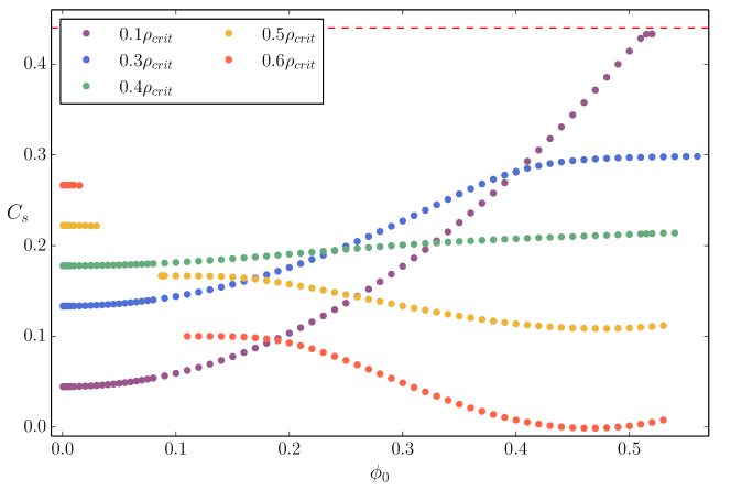
Figure 3: Compactness of constant density objects for $\beta=1$ and different values of $\phi_{0}$. The dashed line shows the GR limit for the compactness, which is obtained only for an object with the critical density $\rho_{crit}$. The density of each solution is indicated by the point color. The gap in the sequence of solutions with $\rho_{0}=0.5\rho_{crit}$ and $\rho_{0}=0.6\rho_{crit}$ is an effect of the scalar field contributions, as explained in the main text.

We fix the radius of the star at a value $R_{s}=1.5$, hence it is convenient to parametrise the density $\rho_{0}$ in terms of the critical density in GR for an object of a given $R_{s}$. We do so by writing $\rho_{0}=A\rho_{crit}$, where $A$ is a constant in the range $(0,1)$ and $\rho_{crit}$ is the critical density of a compact object of constant density in GR (see, e.g., Carroll:2004st ),

$$\rho_{crit}=\frac{16}{3R_{s}^{2}}.$$ (34)

Solutions with $\rho_{0}\geq\rho_{crit}$ do not exist in GR, and we do not find evidence of their existence in the beyond Horndeski model under consideration.

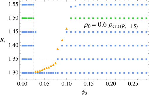
Figure 4: $R_{s}$-$\phi_{0}$ parameter space for a fixed $\rho_{0}$, equal to 60$\%$ of the critical density of an object of radius $R_{s}=1.5$. Green points correspond to the solutions shown in red in Fig. 3. For $R_{s}\gtrsim 1.3$ there is a region of the parameter space where we do not find solutions. The points coloured in orange are referred to in the next Figure.

We apply the results of this numerical method to investigate a physically relevant quantity, the stellar compactness, which allows us to find constraints on the parameters involved, and also to point out differences with GR configurations. The intrinsic stellar compactness, which we plot in Fig. 3, is defined as

$$C_{s}=\frac{m(R_{s})}{R_{s}}.$$ (35)

In the previous expression, the mass of the star $m(R_{s})$ corresponds the value at $R_{s}$ of the the mass function $m(r)$ defined by expressing the metric component $h(r)$ in the stellar interior as

$$h(r)=1-\frac{2m(r)}{r}\,,$$ (36)

that is, including within $m(r)$ all the radial dependence of corrections to the Schwarzschild metric due to matter and scalar field. The compactness defined in this way only includes contributions of the interior of the star – this is why we call it intrinsic – and it is in principle different from the compactness as measured by an asymptotic observer, which we shall discuss in the next subsection. Such difference is important for characterizing the efficiency of the screening mechanism in proximity of the object surface.

Each point in Fig. 3 represents a configuration of matter with radius $R_{s}=1.5$, density indicated by the point colour, $\phi_{0}$ by the $x$-axis, and stellar compactness by the $y$-axis. We observe the following properties:

• High stellar compactness is possible for configurations with a low density of matter: this is due to the large contributions of the scalar profile for characterizing the internal geometry of the system.

• For $\rho_{0}\gtrsim 0.4\rho_{c}$, there exists a range of values of $\phi_{0}$ where we cannot find configurations with the desired radius $R_{s}$. The reasons for this will be explored in some length below.

• The intrinsic stellar compactness does not exceed the GR limit $C=4/9\approx 0.44$ (see, e.g., Carroll:2004st ). This is in contrast to what happens in vector-tensor theories Chagoya:2017fyl , but similar findings have been reported for a subset of Horndeski gravity Maselli:2016gxk . In the next section we show that this is true even when the effects from the exterior solution are taken into account.

The fact that we find a gap in the range of allowed stellar densities is interesting, and deserves some more words since it can suggest ways to test and constrain the parameter space of relativistic compact objects in scalar-tensor theories. We investigate in more detail what happens in the region where we cannot find solutions with $R_{s}=1.5$. We fix the density to be $60\%$ of the critical density: the green points in Fig. 4 correspond to the configurations shown in red in Fig. 3. From $\phi_{0}\approx 0.02$ to $\phi_{0}\approx 0.10$ we do not find solutions with $R_{s}=1.5$. Indeed, around $\phi_{0}\approx 0.02$ there is a drastic change in the maximum radius, which falls to about $R_{s}=1.3$, as shown by the orange points in Fig. 4. The blue points in the same figure show configurations with the same density as the green and orange points, but for different radius: these are drawn in order to outline the region where solutions do not exist.

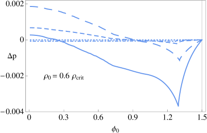
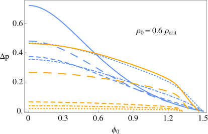
Figure 5: Difference between the pressure in GR and in the beyond Horndeski model under consideration for configurations with $60\%$ of the critical density in GR for an object of radius $R_{s}=1.5$. The left panel shows $\Delta p$ for solutions before the gap along the sequence of green points in Fig. 4, while the right panel corresponds to solutions in the gap (orange curves correspond to orange points in Fig. 4) and along the sequence of green points after the gap.

The origin of an interval in the parameter space where solutions do not exist, and in particular of the drastic change of $R_{s}$ near the lower end of this interval in $\phi_{0}$, can be understood with the help of Fig. 5, where we plot a quantity defined as

$$\Delta p(r) = p(r)-p_{GR}(r)\,,$$ (37)

$$= \xi_{r}^{\,\,r}-G_{r}^{\,\,r}\,,$$

where $\xi_{r}^{\,\,r}$ is the $(r,r)$ component of the left-hand-side of the equations of motion for the metric (see eqs (19) and (22)), while $G_{r}^{\,r}$ the $(r,r)$ component of the Einstein tensor calculated on the configuration we examine, with no contributions from the scalar field (recall we work in units $M_{Pl}=1$). The quantity $\Delta p(r)$ describes the specific contributions to the total pressure which can be associated with the scalar field. The left panel shows $\Delta p$ for solutions with $\phi_{0}<0.02$ and $R_{s}=1.5$; the solid line corresponds to the last configuration along the sequence of green points before the gap in Fig. 4. We see that $\Delta p$ has a minimum at some radius significantly smaller than $R_{s}$. Based on this, we speculate that for $\phi_{0}\gtrsim 0.02$, $\Delta p$ acquires large negative values, whose size is sufficient to drive the total pressure $p(r)$ to zero at a radius smaller than the value $R_{s}\,=\,1.5$, that we initially fix by means of the initial conditions. Since the star radius is defined as the point where the pressure vanishes, the large scalar contribution to the pressure makes the radius smaller than the one we impose. Hence, we learn that there are regions in the parameter space of the scalar-tensor theory under consideration where – due to large contributions associated with the scalar field – there do not exist compact configurations for certain radii and energy densities.

As mentioned above, we can overcome the problem and find solutions by changing some of the conditions, for example by reducing the stellar size $R_{s}$. The physical requirement is that the total pressure vanishes at $R_{s}$. In order to find the correct value of $R_{s}$ where this happens maintaining the same energy density $\rho_{0}$, we thus need to change the central pressure to a smaller value such that both the GR and scalar field contributions to the pressure vanish at the same point. The configurations with maximum radius that we find are shown with orange markers in Fig. 4, and the profiles of $\Delta p$ associated to them are shown with orange lines in the right panel Fig. 5. The curves shown in blue in the same plot instead correspond to configurations along the sequence of green points, to the right of the gap.

These results show that the scalar-tensor theory under consideration imposes more stringent constraints on the stellar properties with respect to GR, since we identified forbidden regions on the the energy density-radius plane, which depend on the value of $\phi_{0}$, and where regular star configurations do not exist. In a more refined version of our analysis, considering a polytropic equation of state, this fact can suggest observable tests for the parameter space of these scalar-tensor theories, which would be excluded in case compact objects are found within the forbidden regions.

IV.3 Matching of interior and exterior solutions

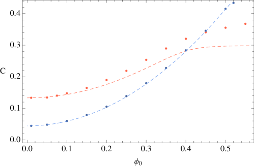
Figure 6: Compactness of constant density configurations for $\beta=1$. The case $\rho_{0}=0.1\rho_{crit}$ is shown in blue, and $\rho_{0}=0.3\rho_{crit}$ in red. The dashed lines show the stellar compactness, and the points show the compactness measured asymptotically. The scalar field can have a relevant impact in the asymptotic compactness, but not enough as to get values of $C$ higher than the GR limit $C\approx 0.44$.

In section III we learned that static, spherically symmetric vacuum solutions to the equations of motion derived from (4) do not correspond exactly to GR configurations in vacuum, since they differ from the Schwarzschild solution by an amount controlled by $\phi_{0}$ and $\beta$. Therefore, the extrinsic compactness measured by an observer far away from a compact object can be different from the intrinsic quantity we studied in Section IV.2, – eq (35) and below – due to contributions from the exterior part of the geometry. To investigate how large these contributions are, we take the very same values of the metric and scalar field at a position $R_{s}$ from the solutions shown found in Section IV.2, and we use these values as initial conditions to integrate numerically the vacuum equations from $R_{s}$ outwards. At large $r$, we compute the gravitational mass using the asymptotic solutions (12)-(13). The matching of the interior and exterior solutions at $R_{s}$ is straightforward, and we match $\phi^{\prime}$, $g_{rr}$, $g^{\prime}_{rr}$ and $g_{tt}$ at that point.

In Fig. 6 we reproduce the intrinsic stellar compactness of configurations with $\rho_{0}=0.1\rho_{crit}$ and $\rho_{0}=0.3\rho_{crit}$ (dashed lines), and we show the asymptotic, extrinsic compactness for some of these configurations (points). Interestingly, even when the effects from the exterior solution are taken into account, the compactness does not exceed the GR limit $C=4/9$. Also, notice that for low density the screening of the exterior solution is highly efficient: even though the scalar field introduces large modifications to the stellar compactness, the scalar contributions in the exterior are negligible, and extrinsic and intrinsic values of the compactness almost coincide. On the other hand, for higher values of the stellar energy density, the values of the extrinsic and intrinsic compactness differ for large values of the parameter $\phi_{0}$. This implies that the effect of the scalar field in this regime is relevant also outside the object, and not only on its interior.

V Discussion

The recent observation of gravitational waves from a neutron star merger GW170817 and its associated electromagnetic counterpart GRB170817A has changed our perspective on scalar-tensor theories. One possibility is to focus only on the simplest theories where the graviton speed $c_{GW}$ is automatically equal to one; the other is to consider richer systems where this condition is obtained at the price of tuning some parameters. In this work we considered the second possibility, studying the physics of compact objects in a theory of beyond Horndeski with $c_{GW}=1$ that includes the scalar kinetic term.

We focussed on black hole and relativistic star configurations which are locally asymptotically flat, that can be continuously connected to GR configurations, and that have been less explored in the literature. Depending on a parameter controlling the scalar field, $\phi_{0}$, our solutions can be very similar to GR when $\phi_{0}$ is small, while they can provide sizeable corrections to it when $\phi_{0}$ is larger. This shows that a Vainshtein screening mechanism, which is very effective to reproduce GR predictions in a weak gravity limit, can be less so in strong gravity regimes.

For what respect black hole configurations, we shown that our geometries are characterized asymptotically by an angular deficit, due to presence of the scalar kinetic term, and are equipped with regular horizons provided that the black hole mass is larger than a value depending on the scalar parameter $\phi_{0}$. Our geometries have not scalar hairs, despite the fact that the scalar has a profile that extends asymptotically far from the black hole. The black hole solutions can be more compact than the Schwarzschild black hole, thanks to the effect of the scalar field. The angular deficit could be detected by its effect on geodesics and light propagation Barriola:1989hx ; Shi:2009nz .

We also studied regular relativistic compact objects corresponding to incompressible stars with constant energy density. The scalar field modifies properties of the star as its compactness, allowing for stars that are twice as compact as neutron stars with the same matter density. These deviations from GR can be accessed observationally, for example through quantities that depend on the tidal deformability of a star, which is directly affected by the compactness Hinderer:2007mb ; Paschalidis:2017qmb . We also found that there are forbidden regions in parameter space where regular star configurations of given radius and energy density cannot be found, depending of the scalar field profile. In a more refined version of our analysis, considering a polytropic equation of state, this fact can suggest observable tests for the parameter space of these scalar-tensor theories, which would be excluded in case objects are found in the forbidden regions.

By analysing the difference between our interior and exterior solutions and their GR counterparts, we numerically investigated the efficiency of the screening of the scalar field inside and outside the relativistic star. We found that including the standard kinetic term of the scalar field breaks the perfect screening of vacuum solutions, not only because of the angular deficit but also because the time and radial components of the metric acquire corrections that distinguish them from the Schwarzschild solution in the exterior of the object. Nevertheless, there are situations where such deviations from a Schwarzschild solution are small in the exterior, while the corrections to the interior metric are large with respect to GR. We cannot find the opposite situation – corrections that are large in the exterior but small in the interior. This indicates that the breaking of screening is more severe in the interior solutions.

Much work is left for the future. It is interesting to continue to investigate the physics of compact objects in other scalar-tensor theories with $c_{GW}=1$, for realistic equations of state for the star interior.

Appendix A Equations of motion

The covariant equations of motion derived from action (4) with $G_{4}=M_{Pl}^{2}+{M_{Pl}^{-2}\beta}\,X$ are

$$0= M_{Pl}^{-2}\beta\left[\phantom{\frac{}{}}[\Phi]R+\nabla_{\alpha}R\nabla^{\alpha}\phi+\frac{R_{\alpha\beta}\langle\Phi\rangle-[\Phi]^{2}\langle\Phi\rangle+\langle\Phi\rangle[\Phi^{2}]+2[\Phi]\langle\Phi^{2}\rangle-2\langle\Phi^{3}\rangle}{X^{2}}\right.$$

$$\left.-\frac{[\Phi]^{3}-3[\Phi]R_{\alpha\beta}\phi^{\alpha}\phi^{\beta}-3[\Phi][\Phi^{2}]-\phi^{\alpha}\phi^{\beta}\phi^{\sigma}\nabla_{\sigma}R_{\alpha\beta}+2[\Phi^{3}]+2R_{\alpha\sigma\beta\delta}\phi^{\alpha}\phi^{\beta}\Phi^{\delta\sigma}}{X}\right]+[\Phi],$$ (38)

$$0= \left(M_{Pl}^{2}+\frac{\beta X}{M_{Pl}^{2}}\right)G_{\mu\nu}-\frac{g_{\mu\nu}X}{2}-\frac{\phi_{\mu}\phi_{\nu}}{2}-\frac{M_{Pl}^{-2}\beta}{4X^{2}}\left(2g_{\mu\nu}\langle\Phi\rangle^{2}-4\phi^{\alpha}\langle\Phi\rangle\Phi_{(\mu|\alpha}\phi_{|\nu)}+2\langle\Phi^{2}\rangle\phi_{\mu}\phi_{\nu}\right)$$

$$-\frac{\beta}{M_{Pl}^{2}}\left[g_{\mu\nu}(\nabla_{\alpha}[\Phi]\phi^{\alpha}+R_{\alpha\beta}\phi^{\alpha}\phi^{\beta}+[\Phi^{2}])-\nabla_{\alpha}\Phi_{\mu\nu}\phi^{\alpha}-\Phi_{\nu\alpha}\Phi^{\alpha}_{\mu}-R_{\mu\alpha\nu\beta}\phi^{\alpha}\phi^{\beta}+\frac{R\phi_{\mu}\phi_{\nu}}{2}\right]$$

$$-\frac{\beta M_{Pl}^{-2}}{2X}\left[g_{\mu\nu}(3\langle\Phi^{2}\rangle+\phi^{\alpha}\phi^{\beta}\nabla_{\sigma}\Phi_{\alpha\beta}\phi^{\sigma})-2\phi^{\alpha}\phi^{\beta}(\Phi_{\mu\alpha}\Phi_{\nu\beta}+\nabla_{\beta}\Phi_{(\mu|\alpha}\phi_{|\nu)})+2[\Phi]\phi^{\alpha}\Phi_{(\mu|\alpha}\phi_{|\nu)}\right.$$

$$\left.-4\Phi_{\beta\alpha}\phi^{\alpha}\Phi^{\beta}{}_{(\mu}\phi_{\nu)}+\phi_{\mu}\phi_{\nu}(2R_{\alpha\beta}\phi^{\alpha}\phi^{\beta}+\nabla_{\alpha}[\Phi]\phi^{\alpha}+2[\Phi^{2}]-[\Phi]^{2})\right]$$ (39)

$$\equiv \,\,\xi_{\mu\nu}\,.$$ (40)

Under the spherically symmetric ansatz (10), the $(r,r)$, $(t,t)$ and $(t,r)$ components of the equations of motion become

$$0= \left(fh\phi_{1}^{\prime}{}^{2}-\phi_{0}^{2}\right)\left(-4fs_{0}+r^{2}\phi_{0}^{2}+f\left(4h+4rh^{\prime}+hr^{2}\phi_{1}^{\prime}{}^{2}\right)\right)+2\beta\left\{\phi_{0}^{4}\left(h-s_{0}+rh^{\prime}\right)\right.$$

$$\left.+2fh\phi_{0}^{2}\phi_{1}^{\prime}\left[\left(2h+3rh^{\prime}\right)\phi_{1}^{\prime}+4hr\phi_{1}^{\prime\prime}\right]-f^{2}h^{2}\phi_{1}^{\prime}{}^{3}\left[\left(h-s_{0}+3rh^{\prime}\right)\phi_{1}^{\prime}+4hr\phi_{1}^{\prime\prime}\right]\right\}\,,$$ (41)

$$0= f\left(\phi_{0}^{2}-fh\phi_{1}^{\prime}{}^{2}\right)\left(4fs_{0}+r^{2}\phi_{0}^{2}+h\left(-4f-4rf^{\prime}+fr^{2}\phi_{1}^{\prime}{}^{2}\right)\right)+2\beta\left\{\phi_{0}^{4}\left(fs_{0}-fh+hrf^{\prime}\right)\right.$$

$$\left.-f^{2}h^{2}\left[fs_{0}+3h\left(f+rf^{\prime}\right)\right]\phi_{1}^{\prime}{}^{4}+2fh^{2}r\phi_{0}^{2}\phi_{1}^{\prime}\left(3f^{\prime}\phi_{1}^{\prime}+2f\phi_{1}^{\prime\prime}\right)\right\}\,,$$ (42)

$$0= \phi_{0}\phi_{1}^{\prime}\left\{fr^{2}\left(fh\phi_{1}^{\prime}{}^{2}-\phi_{0}^{2}\right)+2\beta\left[\phi_{0}^{2}\left(fh-fs_{0}-2hrf^{\prime}+frh^{\prime}\right)+fh\left(fs_{0}+hf+rhf^{\prime}\right)\phi_{1}^{\prime}{}^{2}\right]\right\}\,.$$ (43)

The scalar equation is automatically satisfied by the algebraic solution to eq. (43) for $\phi^{\prime}$.

References

- (1) T. Clifton, P. G. Ferreira, A. Padilla and C. Skordis, Phys. Rept. 513 (2012) 1 doi:10.1016/j.physrep.2012.01.001 [arXiv:1106.2476 [astro-ph.CO]].
- (2) A. Wang, Int. J. Mod. Phys. D 26 (2017) no.07, 1730014 doi:10.1142/S0218271817300142 [arXiv:1701.06087 [gr-qc]].
- (3) L. Amendola, Phys. Lett. B 301 (1993) 175 doi:10.1016/0370-2693(93)90685-B [gr-qc/9302010].
- (4) R. Kimura, T. Kobayashi and K. Yamamoto, Phys. Rev. D 85 (2012) 024023 doi:10.1103/PhysRevD.85.024023 [arXiv:1111.6749 [astro-ph.CO]].
- (5) E. Bellini, R. Jimenez and L. Verde, JCAP 1505 (2015) no.05, 057 doi:10.1088/1475-7516/2015/05/057 [arXiv:1504.04341 [astro-ph.CO]].
- (6) E. Babichev and C. Deffayet, Class. Quant. Grav. 30 (2013) 184001 doi:10.1088/0264-9381/30/18/184001 [arXiv:1304.7240 [gr-qc]].
- (7) C. Brans and R. H. Dicke, Phys. Rev. 124 (1961) 925. doi:10.1103/PhysRev.124.925
- (8) A. Nicolis, R. Rattazzi and E. Trincherini, Phys. Rev. D 79 (2009) 064036 doi:10.1103/PhysRevD.79.064036 [arXiv:0811.2197 [hep-th]].
- (9) G. W. Horndeski, Int. J. Theor. Phys. 10 (1974) 363. doi:10.1007/BF01807638
- (10) J. Gleyzes, D. Langlois, F. Piazza and F. Vernizzi, Phys. Rev. Lett. 114 (2015) no.21, 211101 doi:10.1103/PhysRevLett.114.211101 [arXiv:1404.6495 [hep-th]].
- (11) D. Langlois and K. Noui, JCAP 1602 (2016) no.02, 034 doi:10.1088/1475-7516/2016/02/034 [arXiv:1510.06930 [gr-qc]].
- (12) M. Crisostomi, K. Koyama and G. Tasinato, JCAP 1604 (2016) no.04, 044 doi:10.1088/1475-7516/2016/04/044 [arXiv:1602.03119 [hep-th]].
- (13) J. Ben Achour, M. Crisostomi, K. Koyama, D. Langlois, K. Noui and G. Tasinato, JHEP 1612 (2016) 100 doi:10.1007/JHEP12(2016)100 [arXiv:1608.08135 [hep-th]].
- (14) M. Crisostomi, M. Hull, K. Koyama and G. Tasinato, JCAP 1603 (2016) no.03, 038 doi:10.1088/1475-7516/2016/03/038 [arXiv:1601.04658 [hep-th]].
- (15) M. Zumalac rregui and J. Garc a-Bellido, Phys. Rev. D 89 (2014) 064046 doi:10.1103/PhysRevD.89.064046 [arXiv:1308.4685 [gr-qc]].
- (16) C. A. R. Herdeiro and E. Radu, Int. J. Mod. Phys. D 24 (2015) no.09, 1542014 doi:10.1142/S0218271815420146 [arXiv:1504.08209 [gr-qc]].
- (17) J. Sakstein, Phys. Rev. D 92 (2015) 124045 doi:10.1103/PhysRevD.92.124045 [arXiv:1511.01685 [astro-ph.CO]].
- (18) H. O. Silva, A. Maselli, M. Minamitsuji and E. Berti, Int. J. Mod. Phys. D 25 (2016) no.09, 1641006 doi:10.1142/S0218271816410066 [arXiv:1602.05997 [gr-qc]].
- (19) J. Sakstein, E. Babichev, K. Koyama, D. Langlois and R. Saito, Phys. Rev. D 95 (2017) no.6, 064013 doi:10.1103/PhysRevD.95.064013 [arXiv:1612.04263 [gr-qc]].
- (20) C. A. R. Herdeiro and E. Radu, Int. J. Mod. Phys. D 24 (2015) no.09, 1542014 doi:10.1142/S0218271815420146 [arXiv:1504.08209 [gr-qc]].
- (21) J. D. Bekenstein, In *Moscow 1996, 2nd International A.D. Sakharov Conference on physics* 216-219 [gr-qc/9605059].
- (22) E. Babichev, C. Charmousis and A. Leh bel, Class. Quant. Grav. 33 (2016) no.15, 154002 doi:10.1088/0264-9381/33/15/154002 [arXiv:1604.06402 [gr-qc]].
- (23) E. Babichev, C. Charmousis and A. Leh bel, JCAP 1704 (2017) no.04, 027 doi:10.1088/1475-7516/2017/04/027 [arXiv:1702.01938 [gr-qc]].
- (24) T. Damour and G. Esposito-Farese, Phys. Rev. Lett. 70 (1993) 2220. doi:10.1103/PhysRevLett.70.2220
- (25) T. Damour and G. Esposito-Farese, Phys. Rev. D 54 (1996) 1474 doi:10.1103/PhysRevD.54.1474 [gr-qc/9602056].
- (26) M. Salgado, D. Sudarsky and U. Nucamendi, Phys. Rev. D 58 (1998) 124003 doi:10.1103/PhysRevD.58.124003 [gr-qc/9806070].
- (27) J. Chagoya, K. Koyama, G. Niz and G. Tasinato, JCAP 1410 (2014) no.10, 055 doi:10.1088/1475-7516/2014/10/055 [arXiv:1407.7744 [hep-th]].
- (28) T. Kobayashi, Y. Watanabe and D. Yamauchi, Phys. Rev. D 91 (2015) no.6, 064013 doi:10.1103/PhysRevD.91.064013 [arXiv:1411.4130 [gr-qc]].
- (29) H. O. Silva, J. Sakstein, L. Gualtieri, T. P. Sotiriou and E. Berti, arXiv:1711.02080 [gr-qc].
- (30) M. Crisostomi and K. Koyama, Phys. Rev. D 97 (2018) no.2, 021301 doi:10.1103/PhysRevD.97.021301 [arXiv:1711.06661 [astro-ph.CO]].
- (31) A. Dima and F. Vernizzi, arXiv:1712.04731 [gr-qc].
- (32) A. Maselli, H. O. Silva, M. Minamitsuji and E. Berti, Phys. Rev. D 93 (2016) no.12, 124056 doi:10.1103/PhysRevD.93.124056 [arXiv:1603.04876 [gr-qc]].
- (33) E. Babichev, K. Koyama, D. Langlois, R. Saito and J. Sakstein, Class. Quant. Grav. 33 (2016) no.23, 235014 doi:10.1088/0264-9381/33/23/235014 [arXiv:1606.06627 [gr-qc]].
- (34) A. Cisterna, T. Delsate and M. Rinaldi, Phys. Rev. D 92 (2015) no.4, 044050 doi:10.1103/PhysRevD.92.044050 [arXiv:1504.05189 [gr-qc]].
- (35) P. Pani and E. Berti, Phys. Rev. D 90 (2014) no.2, 024025 doi:10.1103/PhysRevD.90.024025 [arXiv:1405.4547 [gr-qc]].
- (36) G. Pappas and T. P. Sotiriou, Phys. Rev. D 91 (2015) no.4, 044011 doi:10.1103/PhysRevD.91.044011 [arXiv:1412.3494 [gr-qc]].
- (37) T. Gupta, B. Majumder, K. Yagi and N. Yunes, Class. Quant. Grav. 35 (2018) no.2, 025009 doi:10.1088/1361-6382/aa9c68 [arXiv:1710.07862 [gr-qc]].
- (38) B. P. Abbott et al. [LIGO Scientific and Virgo Collaborations], Phys. Rev. Lett. 119 (2017) no.16, 161101 doi:10.1103/PhysRevLett.119.161101 [arXiv:1710.05832 [gr-qc]].
- (39) B. P. Abbott et al. [LIGO Scientific and Virgo and Fermi-GBM and INTEGRAL Collaborations], Astrophys. J. 848 (2017) no.2, L13 doi:10.3847/2041-8213/aa920c [arXiv:1710.05834 [astro-ph.HE]].
- (40) J. M. Ezquiaga and M. Zumalacárregui, Phys. Rev. Lett. 119 (2017) no.25, 251304 doi:10.1103/PhysRevLett.119.251304 [arXiv:1710.05901 [astro-ph.CO]].
- (41) P. Creminelli and F. Vernizzi, Phys. Rev. Lett. 119 (2017) no.25, 251302 doi:10.1103/PhysRevLett.119.251302 [arXiv:1710.05877 [astro-ph.CO]].
- (42) J. Sakstein and B. Jain, Phys. Rev. Lett. 119 (2017) no.25, 251303 doi:10.1103/PhysRevLett.119.251303 [arXiv:1710.05893 [astro-ph.CO]].
- (43) T. Baker, E. Bellini, P. G. Ferreira, M. Lagos, J. Noller and I. Sawicki, Phys. Rev. Lett. 119 (2017) no.25, 251301 doi:10.1103/PhysRevLett.119.251301 [arXiv:1710.06394 [astro-ph.CO]].
- (44) T. Kobayashi, M. Yamaguchi and J. Yokoyama, Prog. Theor. Phys. 126 (2011) 511 doi:10.1143/PTP.126.511 [arXiv:1105.5723 [hep-th]].
- (45) C. Deffayet, X. Gao, D. A. Steer and G. Zahariade, Phys. Rev. D 84 (2011) 064039 doi:10.1103/PhysRevD.84.064039 [arXiv:1103.3260 [hep-th]].
- (46) D. Bettoni, J. M. Ezquiaga, K. Hinterbichler and M. Zumalacárregui, Phys. Rev. D 95 (2017) no.8, 084029 doi:10.1103/PhysRevD.95.084029 [arXiv:1608.01982 [gr-qc]].
- (47) B. M. Gripaios, JHEP 0410 (2004) 069 doi:10.1088/1126-6708/2004/10/069 [hep-th/0408127].
- (48) G. Tasinato, JHEP 1404, 067 (2014) doi:10.1007/JHEP04(2014)067 [arXiv:1402.6450 [hep-th]].
- (49) L. Heisenberg, JCAP 1405, 015 (2014) doi:10.1088/1475-7516/2014/05/015 [arXiv:1402.7026 [hep-th]].
- (50) J. Chagoya, G. Niz and G. Tasinato, Class. Quant. Grav. 33 (2016) no.17, 175007 doi:10.1088/0264-9381/33/17/175007 [arXiv:1602.08697 [hep-th]].
- (51) E. Babichev and C. Charmousis, JHEP 1408 (2014) 106 doi:10.1007/JHEP08(2014)106 [arXiv:1312.3204 [gr-qc]].
- (52) L. Heisenberg, R. Kase, M. Minamitsuji and S. Tsujikawa, JCAP 1708 (2017) no.08, 024 doi:10.1088/1475-7516/2017/08/024 [arXiv:1706.05115 [gr-qc]].
- (53) J. Chagoya, G. Niz and G. Tasinato, Class. Quant. Grav. 34 (2017) no.16, 165002 doi:10.1088/1361-6382/aa7c01 [arXiv:1703.09555 [gr-qc]].
- (54) K. Koyama and J. Sakstein, Phys. Rev. D 91 (2015) 124066 doi:10.1103/PhysRevD.91.124066 [arXiv:1502.06872 [astro-ph.CO]].
- (55) R. Saito, D. Yamauchi, S. Mizuno, J. Gleyzes and D. Langlois, JCAP 1506 (2015) 008 doi:10.1088/1475-7516/2015/06/008 [arXiv:1503.01448 [gr-qc]].
- (56) A. Achucarro, R. Gregory and K. Kuijken, Phys. Rev. D 52 (1995) 5729 doi:10.1103/PhysRevD.52.5729 [gr-qc/9505039].
- (57) A. De Felice, R. Kase and S. Tsujikawa, Phys. Rev. D 92 (2015) no.12, 124060 doi:10.1103/PhysRevD.92.124060 [arXiv:1508.06364 [gr-qc]].
- (58) M. Rinaldi, Phys. Rev. D 86 (2012) 084048 doi:10.1103/PhysRevD.86.084048 [arXiv:1208.0103 [gr-qc]].
- (59) M. Aryal, L. H. Ford and A. Vilenkin, Phys. Rev. D 34 (1986) 2263. doi:10.1103/PhysRevD.34.2263
- (60) U. Nucamendi and D. Sudarsky, Class. Quant. Grav. 14 (1997) 1309 doi:10.1088/0264-9381/14/5/031 [gr-qc/9611043].
- (61) M. Barriola and A. Vilenkin, Phys. Rev. Lett. 63 (1989) 341. doi:10.1103/PhysRevLett.63.341
- (62) X. Shi and X. z. Li, Class. Quant. Grav. 8 (1991) 761 doi:10.1088/0264-9381/8/4/019 [arXiv:0903.3085 [gr-qc]].
- (63) R. Kase, S. Tsujikawa and A. De Felice, JCAP 1603 (2016) no.03, 003 doi:10.1088/1475-7516/2016/03/003 [arXiv:1512.06497 [gr-qc]].
- (64) L. Heisenberg, R. Kase and S. Tsujikawa, Phys. Rev. D 94 (2016) no.12, 123513 doi:10.1103/PhysRevD.94.123513 [arXiv:1608.08390 [gr-qc]].
- (65) O. J. Tattersall, P. G. Ferreira and M. Lagos, arXiv:1802.08606 [gr-qc].
- (66) R. C. Tolman, Phys. Rev. 55 (1939) 364. doi:10.1103/PhysRev.55.364
- (67) S. M. Carroll, San Francisco, USA: Addison-Wesley (2004) 513 p
- (68) T. Hinderer, Astrophys. J. 677 (2008) 1216 doi:10.1086/533487 [arXiv:0711.2420 [astro-ph]].
- (69) V. Paschalidis, K. Yagi, D. Alvarez-Castillo, D. B. Blaschke and A. Sedrakian, arXiv:1712.00451 [astro-ph.HE].
- (70)